Quantum Information and Computation for Chemistry 154_Chap1.pdfINTRODUCTION TO QUANTUM INFORMATION AND COMPUTATION FOR CHEMISTRY SABREKAIS Department of Chemistry and Physics, Purdue

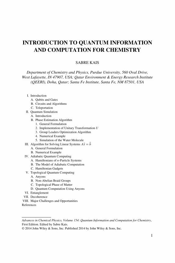
INTRODUCTION TO QUANTUM INFORMATIONAND COMPUTATION FOR CHEMISTRY

SABRE KAIS

Department of Chemistry and Physics, Purdue University, 560 Oval Drive,West Lafayette, IN 47907, USA; Qatar Environment & Energy Research Institute

(QEERI), Doha, Qatar; Santa Fe Institute, Santa Fe, NM 87501, USA

I. IntroductionA. Qubits and GatesB. Circuits and AlgorithmsC. Teleportation

II. Quantum SimulationA. IntroductionB. Phase Estimation Algorithm

1. General Formulation2. Implementation of Unitary Transformation U

3. Group Leaders Optimization Algorithm4. Numerical Example5. Simulation of the Water Molecule

III. Algorithm for Solving Linear Systems A�x = �bA. General FormulationB. Numerical Example

IV. Adiabatic Quantum ComputingA. Hamiltonians of n-Particle SystemsB. The Model of Adiabatic ComputationC. Hamiltonian Gadgets

V. Topological Quantum ComputingA. AnyonsB. Non-Abelian Braid GroupsC. Topological Phase of MatterD. Quantum Computation Using Anyons

VI. EntanglementVII. Decoherence

VIII. Major Challenges and OpportunitiesReferences

Advances in Chemical Physics, Volume 154: Quantum Information and Computation for Chemistry,First Edition. Edited by Sabre Kais.© 2014 John Wiley & Sons, Inc. Published 2014 by John Wiley & Sons, Inc.

1

2 SABRE KAIS

I. INTRODUCTION

The development and use of quantum computers for chemical applications hasthe potential for revolutionary impact on the way computing is done in the fu-ture [1–7]. Major challenge opportunities are abundant (see next fifteen chapters).One key example is developing and implementing quantum algorithms for solvingchemical problems thought to be intractable for classical computers. Other chal-lenges include the role of quantum entanglement, coherence, and superpositionin photosynthesis and complex chemical reactions. Theoretical chemists have en-countered and analyzed these quantum effects from the view of physical chemistryfor decades. Therefore, combining results and insights from the quantum infor-mation community with those of the chemical physics community might lead to afresh understanding of important chemical processes. In particular, we will discussthe role of entanglement in photosynthesis, in dissociation of molecules, and in themechanism with which birds determine magnetic north. This chapter is intendedto survey some of the most important recent results in quantum computation andquantum information, with potential applications in quantum chemistry. To startwith, we give a comprehensive overview of the basics of quantum computing(the gate model), followed by introducing quantum simulation, where the phaseestimation algorithm (PEA) plays a key role. Then we demonstrate how PEA com-bined with Hamiltonian simulation and multiplicative inversion can enable us tosolve some types of linear systems of equations described by A�x = �b. Then oursubject turns from gate model quantum computing (GMQC) to adiabatic quantumcomputing (AQC) and topological quantum computing, which have gained in-creasing attention in the recent years due to their rapid progress in both theoreticaland experimental areas. Finally, applications of the concepts of quantum infor-mation theory are usually related to the powerful and counter intuitive quantummechanical effects of superposition, interference, and entanglement.

Throughout history, man has learned to build tools to aid computation. Fromabacuses to digital microprocessors, these tools epitomize the fact that laws ofphysics support computation. Therefore, a natural question arises: “Which physi-cal laws can we use for computation?” For a long period of time, questions suchas this were not considered relevant because computation devices were built ex-clusively based on classical physics. It was not until the 1970s and 1980s whenFeynmann [8], Deutsch [9], Benioff [10], and Bennett [11] proposed the idea ofusing quantum mechanics to perform calculation that the possibility of building aquantum computing device started to gain some attention.

What they conjectured then is what we call today a quantum computer. Aquantum computer is a device that takes direct advantage of quantum mechani-cal phenomena such as superposition and entanglement to perform calculations[12]. Because they compute in ways that classical computers cannot, for certainproblems quantum algorithms provide exponential speedups over their classical

INTRODUCTION TO QUANTUM INFORMATION 3

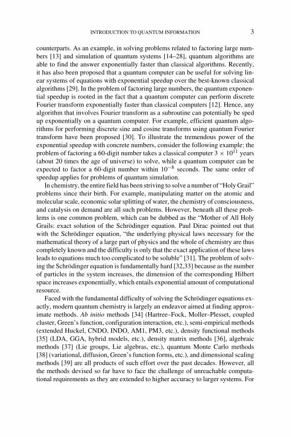
counterparts. As an example, in solving problems related to factoring large num-bers [13] and simulation of quantum systems [14–28], quantum algorithms areable to find the answer exponentially faster than classical algorithms. Recently,it has also been proposed that a quantum computer can be useful for solving lin-ear systems of equations with exponential speedup over the best-known classicalalgorithms [29]. In the problem of factoring large numbers, the quantum exponen-tial speedup is rooted in the fact that a quantum computer can perform discreteFourier transform exponentially faster than classical computers [12]. Hence, anyalgorithm that involves Fourier transform as a subroutine can potentially be spedup exponentially on a quantum computer. For example, efficient quantum algo-rithms for performing discrete sine and cosine transforms using quantum Fouriertransform have been proposed [30]. To illustrate the tremendous power of theexponential speedup with concrete numbers, consider the following example: theproblem of factoring a 60-digit number takes a classical computer 3 × 1011 years(about 20 times the age of universe) to solve, while a quantum computer can beexpected to factor a 60-digit number within 10−8 seconds. The same order ofspeedup applies for problems of quantum simulation.

In chemistry, the entire field has been striving to solve a number of “Holy Grail”problems since their birth. For example, manipulating matter on the atomic andmolecular scale, economic solar splitting of water, the chemistry of consciousness,and catalysis on demand are all such problems. However, beneath all these prob-lems is one common problem, which can be dubbed as the “Mother of All HolyGrails: exact solution of the Schrodinger equation. Paul Dirac pointed out thatwith the Schrodinger equation, “the underlying physical laws necessary for themathematical theory of a large part of physics and the whole of chemistry are thuscompletely known and the difficulty is only that the exact application of these lawsleads to equations much too complicated to be soluble” [31]. The problem of solv-ing the Schrodinger equation is fundamentally hard [32,33] because as the numberof particles in the system increases, the dimension of the corresponding Hilbertspace increases exponentially, which entails exponential amount of computationalresource.

Faced with the fundamental difficulty of solving the Schrodinger equations ex-actly, modern quantum chemistry is largely an endeavor aimed at finding approx-imate methods. Ab initio methods [34] (Hartree–Fock, Moller–Plesset, coupledcluster, Green’s function, configuration interaction, etc.), semi-empirical methods(extended Huckel, CNDO, INDO, AM1, PM3, etc.), density functional methods[35] (LDA, GGA, hybrid models, etc.), density matrix methods [36], algebraicmethods [37] (Lie groups, Lie algebras, etc.), quantum Monte Carlo methods[38] (variational, diffusion, Green’s function forms, etc.), and dimensional scalingmethods [39] are all products of such effort over the past decades. However, allthe methods devised so far have to face the challenge of unreachable computa-tional requirements as they are extended to higher accuracy to larger systems. For

4 SABRE KAIS

example, in the case of full CI calculation, for N orbitals and m electrons thereare Cm

N ≈ Nm

m! ways to allocate electrons among orbitals. Doing full configurationinteraction (FCI) calculations for methanol (CH3OH) using 6-31G (18 electronsand 50 basis functions) requires about 1017 configurations. This task is impossibleon any current computer. One of the largest FCI calculations reported so far hasabout 109 configurations (1.3 billion configurations for Cr2 molecules [40]).

However, due to exponential speedup promised by quantum computers, suchsimulation can be accomplished within only polynomial amount of time, which isreasonable for most applications. As we will show later, using the phase estimationalgorithm, one is able to calculate eigenvalues of a given Hamiltonian H in timethat is polynomial in O(log N), where N is the size of the Hamiltonian. So inthis sense, quantum computation and quantum information will have enormousimpact on quantum chemistry by enabling quantum chemists and physicists tosolve problems beyond the processing power of classical computers.

The importance of developing quantum computers derives not only from thediscipline of quantum physics and chemistry alone, but also from a wider contextof computer science and the semiconductor electronics industry. Since 1946, theprocessing power of microprocessors has doubled every year simply due to theminiaturization of basic electronic components on a chip. The number of transistorson a single integrated circuit chip doubled every 18 months, which is a fact knownas Moore’s law. This exponential growth in the processing power of classical com-puters has spurred revolutions in every area of science and engineering. However,the trend cannot last forever. In fact, it is projected that by the year 2020 the size ofa transistor would be on the order of a single atom. At that scale, classical lawsof physics no longer hold and the behavior of the circuit components obeys lawsof quantum mechanics, which implies that a new paradigm is needed to exploitthe effects of quantum mechanics to perform computation, or in a more generalsense, information processing tasks. Hence, the mission of quantum computing isto study how information can be processed with quantum mechanical devices aswell as what kinds of tasks beyond the capabilities of classical computers can beperformed efficiently on these devices.

Accompanying the tremendous promises of quantum computers are the exper-imental difficulties of realizing one that truly meets its above-mentioned theoret-ical potential. Despite the ongoing debate on whether building a useful quantumcomputer is possible, no fundamental physical principles are found to prevent aquantum computer from being built. Engineering issues, however, remain. Theimprovement and realization of quantum computers are largely interdisciplinaryefforts. The disciplines that contribute to quantum computing, or more generallyquantum information processing, include quantum physics, mathematics, com-puter science, solid-state device physics, mesoscopic physics, quantum devices,device technology, quantum optics, optical communication, and nuclear magneticresonance (NMR), to name just a few.


A. Qubits and Gates

In general, we can think of information as something that can be encoded in thestate of a physical system. If the physical system obeys classical laws of physics,such as a classical computer, the information stored there is of “classical” nature.To quantify information, the concept of bit has been introduced and defined as thebasic unit of information. A bit of information stored in a classical computer is avalue 0 or 1 kept in a certain location of the memory unit. The computer is able tomeasure the bit and retrieve the information without changing the state of the bit.If the bit is at the same state every time it is measured, it will yield the same results.A bit can also be copied and one can prepare another bit with the same state. Astring of bits represents one single number.

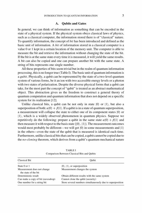
All these properties of bits seem trivial but in the realm of quantum informationprocessing, this is no longer true (Table I). The basic unit of quantum information isa qubit. Physically, a qubit can be represented by the state of a two-level quantumsystem of various forms, be it an ion with two accessible energy levels or a photonwith two states of polarization. Despite the diverse physical forms that a qubit cantake, for the most part the concept of “qubit” is treated as an abstract mathematicalobject. This abstraction gives us the freedom to construct a general theory ofquantum computation and quantum information that does not depend on a specificsystem for its realization [12].

Unlike classical bits, a qubit can be not only in state |0〉 or |1〉, but also asuperposition of both: α|0〉 + β|1〉. If a qubit is in a state of quantum superposition,a measurement will collapse the state to either one of its component states |0〉 or|1〉, which is a widely observed phenomenon in quantum physics. Suppose werepetitively do the following: prepare a qubit in the same state α|0〉 + β|1〉 andthen measure it with respect to the basis state {|0〉, |1〉}. The measurement outcomeswould most probably be different—we will get |0〉 in some measurements and |1〉in the others—even the state of the qubit that is measured is identical each time.Furthermore, unlike classical bits that can be copied, a qubit cannot be copied due tothe no-cloning theorem, which derives from a qubit’s quantum mechanical nature

TABLE IComparison Between Classical Bits and Qubits

Classical Bit Qubit

State 0 or 1 |0〉, |1〉, or superpositionMeasurement does not change Measurement changes the system

the state of the bitDeterministic result Obtain different results with the same systemCan make a copy of bit (eavesdrop) Cannot clone the qubit (security)One number for a string bit Store several numbers simultaneously due to superposition

6 SABRE KAIS

(see Ref. [12], p. 24 for details). Such no-cloning property of a qubit has been usedfor constructing security communication devices, because a qubit of information isimpossible to eavesdrop. In terms of information storage, since a qubit or an arrayof qubits could be in states of quantum superposition such as α00|00〉 + α01|01〉 +α10|10〉 + α11|11〉, a string of qubits is able to store several numbers α00, α01, . . .

simultaneously, while a classical string of bits can only represent a single number.In this sense, n qubits encode not n bits of classical information, but 2n numbers.In spite of the fact that none of the 2n numbers are efficiently accessible becausea measurement will destroy the state of superposition, this exponentially largeinformation processing space combined with the peculiar mathematical structureof quantum mechanics still implies the formidable potential in the performance ofsome of computational tasks exponentially faster than classical computers.

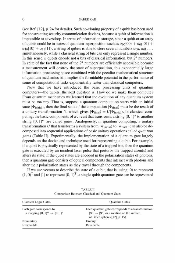
Now that we have introduced the basic processing units of quantumcomputers—the qubits, the next question is: How do we make them compute?From quantum mechanics we learned that the evolution of any quantum systemmust be unitary. That is, suppose a quantum computation starts with an initialstate |�initial〉, then the final state of the computation |�final〉 must be the result ofa unitary transformation U, which gives |�final〉 = U|�initial〉. In classical com-puting, the basic components of a circuit that transforms a string {0, 1}n to anotherstring {0, 1}m are called gates. Analogously, in quantum computing, a unitarytransformation U that transforms a system from |�initial〉 to |�final〉 can also be de-composed into sequential applications of basic unitary operations called quantum

gates (Table II). Experimentally, the implementation of a quantum gate largelydepends on the device and technique used for representing a qubit. For example,if a qubit is physically represented by the state of a trapped ion, then the quantumgate is executed by an incident laser pulse that perturbs the trapped atom(s) andalters its state; if the qubit states are encoded in the polarization states of photons,then a quantum gate consists of optical components that interact with photons andalter their polarization states as they travel through the components.

If we use vectors to describe the state of a qubit, that is, using |0〉 to represent(1, 0)T and |1〉 to represent (0, 1)T, a single-qubit quantum gate can be represented

TABLE IIComparison Between Classical and Quantum Gates

Classical Logic Gates Quantum Gates

Each gate corresponds to Each quantum gate corresponds to a transformationa mapping {0, 1}m → {0, 1}n |�〉 → |�′〉 or a rotation on the surface

of Bloch sphere ([12], p. 15)Nonunitary UnitaryIrreversible Reversible


using a 2 × 2 matrix. For example, a quantum NOT gate can be represented bythe Pauli X matrix

UNOT = X =(

0 1

1 0

)(1)

To see how this works, note that X|0〉 = |1〉 and X|1〉 = |0〉. Therefore, thesheer effect of applying X to a qubit is to flip its state from |0〉 to |1〉. This isjust one example of single-qubit gates. Other commonly used gates include theHadamard gate H , Z rotation gate, phase gate S, and π

8 gate T :

H = 1√2

(1 1

1 −1

), S =

(1 0

0 i

), T =

(1 0

0 eiπ/4

)(2)

If a quantum gate involves two qubits, then it is represented by a 4 × 4 matrix.The state of a two-qubit system is generally in form of α00|00〉 + α01|01〉 +α10|10〉 + α11|11〉, which can be written as a vector (α00, α01, α10, α11)T. In matrixform, the CNOT gate is defined as

UCNOT =

⎛⎜⎜⎜⎝

1 0 0 0

0 1 0 0

0 0 0 1

0 0 1 0

⎞⎟⎟⎟⎠ (3)

It is easy to verify that applying CNOT gate to a state |�0〉 = α00|00〉 +α01|01〉 + α10|10〉 + α11|11〉 results in a state

UCNOT|�0〉 = α00|00〉 + α01|01〉 + α10|11〉 + α11|10〉 (4)

Hence, the effect of a CNOT gate is equivalent to a conditional X gate: If thefirst qubit is in |0〉, then the second qubit remains intact; on the other hand, if thefirst qubit is in |1〉, then the second qubit is flipped. Generally, the first qubit iscalled the control and the second is the target.

In classical computing, an arbitrary mapping {0, 1}n → {0, 1}m can be executedby a sequence of basic gates such as AND, OR, NOT, and so on. Similarly inquantum computing, an arbitrary unitary transformation U can also be decomposedas a product of basic quantum gates. A complete set of such basic quantum gates isa universal gate set. For example, Hadamard, phase, CNOT, and π/8 gates forma universal gate set ([12], p. 194).

Now that we have introduced the concepts of qubits and quantum gates andcompared them with their classical counterpart, we can see that they are the verybuilding blocks of a quantum computer. However, it turns out that having qubitsand executable universal gates is not enough for building a truly useful quantum

8 SABRE KAIS

computer that delivers its theoretical promises. So what does it really take to buildsuch a quantum computer? A formal answer to this question is the following sevencriteria proposed by DiVincenzo [41]:

• A scalable physical system with well-characterized qubits.• The ability to initialize the state of the qubits to a simple fiducial state.• Long (relative) decoherence times, much longer than the gate operation time.• A universal set of quantum gates.• A qubit-specific measurement capability.• The ability to inter convert stationary and flying qubits.• The ability to faithfully transmit flying qubits between specified locations.

For a detailed review of state-of-the-art experimental implementation based onthe preceding criteria, refer to Ref. [42]. The take-home message is that it is clearthat we can gain some advantage by storing, transmitting, and processing informa-tion encoded in systems that exhibit unique quantum properties, and a number ofphysical systems are currently being developed for quantum computation. How-ever, it remains unclear which technology, if any, will ultimately prove successfulin building a scalable quantum computer.

B. Circuits and Algorithms

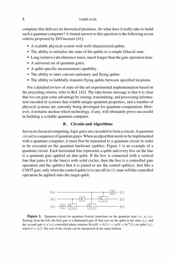
Just as in classical computing, logic gates are cascaded to form a circuit. A quantumcircuit is a sequence of quantum gates. When an algorithm needs to be implementedwith a quantum computer, it must first be translated to a quantum circuit in orderto be executed on the quantum hardware (qubits). Figure 1 is an example of aquantum circuit. Each horizontal line represents a qubit and every box on the lineis a quantum gate applied on that qubit. If the box is connected with a verticalline that joins it to the line(s) with solid circles, then the box is a controlled gateoperation and the qubit(s) that it is joined to are the control qubit(s). Just like aCNOT gate, only when the control qubit (s) is (are all) in |1〉 state will the controlledoperation be applied onto the target qubit.

x3〉 • • H y1〉||

|

|

|

|

x2〉 • H Rπ/2 y2〉

x1〉 H Rπ/2 Rπ/4 y3〉

Figure 1. Quantum circuit for quantum Fourier transform on the quantum state |x1, x2, x3〉.Starting from the left, the first gate is a Hadamard gate H that acts on the qubit in the state |x1〉, andthe second gate is a |x2〉-controlled phase rotation Rθ(a|0〉 + b|1〉) → (a|0〉 + beiθ |1〉) on qubit |x1〉,where θ = π/2. The rest of the circuit can be interpreted in the same fashion.


C. Teleportation

Quantum teleportation exploits some of the most basic and unique features of quan-tum mechanics, which is quantum entanglement, essentially implies an intriguingproperty that two quantum correlated systems cannot be considered independenteven if they are far apart. The dream of teleportation is to be able to travel bysimply reappearing at some distant location. Teleportation of a quantum state en-compasses the complete transfer of information from one particle to another. Thecomplete specification of a quantum state of a system generally requires an infiniteamount of information, even for simple two-level systems (qubits). Moreover, theprinciples of quantum mechanics dictate that any measurement on a system imme-diately alters its state, while yielding at most one bit of information. The transferof a state from one system to another (by performing measurements on the firstand operations on the second) might therefore appear impossible. However, it wasshown that the property of entanglement in quantum mechanics, in combinationwith classical communication, can be used to teleport quantum states. Althoughteleportation of large objects still remains a fantasy, quantum teleportation hasbecome a laboratory reality for photons, electrons, and atoms [43–52].

More precisely, quantum teleportation is a quantum protocol by which the in-formation on a qubit A is transmitted exactly (in principle) to another qubit B. Thisprotocol requires a conventional communication channel capable of transmittingtwo classical bits, and an entangled pair (B, C) of qubits, with C at the locationof origin with A and B at the destination. The protocol has three steps: measureA and C jointly to yield two classical bits; transmit the two bits to the other endof the channel; and use the two bits to select one of the four ways of recovering B

[53,54].Efficient long-distance quantum teleportation is crucial for quantum commu-

nication and quantum networking schemes. Ursin and coworkers [55] have per-formed a high-fidelity teleportation of photons over a distance of 600 m across theRiver Danube in Vienna, with the optimal efficiency that can be achieved using lin-ear optics. Another exciting experiment in quantum communication has also beendone with one photon that is measured locally at the Canary Island of La Palma,whereas the other is sent over an optical free-space link to Tenerife, where the Op-tical Ground Station of the European Space Agency acts as the receiver [55,56].This exceeds previous free-space experiments by more than an order of magni-tude in distance, and is an essential step toward future satellite-based quantumcommunication.

Recently, we have proposed a scheme for implementing quantum teleportationin a three-electron systems [52]. For more electrons, using Hubbard Hamiltonian,in the limit of the Coulomb repulsion parameter for electrons on the same siteU → +∞, there is no double occupation in the magnetic field; the system isreduced to the Heisenberg model. The neighboring spins will favor the anti parallel

10 SABRE KAIS

configuration for the ground state. If the spin at one end is flipped, then the spins onthe whole chain will be flipped accordingly due to the spin–spin correlation. Suchthat the spins at the two ends of the chain are entangled, a spin entanglement canbe used for quantum teleportation, and the information can be transferred throughthe chain. This might be an exciting new direction for teleportation in molecularchains [57].

II. QUANTUM SIMULATION

A. Introduction

As already mentioned, simulating quantum systems by exact solution of theSchrodinger equation is a fundamentally hard task that the quantum chemistry com-munity has been trying to tackle for decades with only approximate approaches.The key challenges of quantum simulation include the following (see next fivechapters) [28]:

1. Isolate qubits in physical systems. For example, in a photonic quantum com-puter simulating a hydrogen molecule, the logical states |0〉 and |1〉 corre-spond to horizontal |H〉 and vertical |V 〉 polarization states [58].

2. Represent the Hamiltonian H . This is to write H as a sum of Hermitianoperators, each to be converted into unitary gates under the exponentialmap.

3. Prepare the states |ψ〉. By direct mapping, each qubit represents the fermionicoccupation state of a particular orbital. Fock space of the system is mappedonto the Hilbert space of qubits.

4. Extract the energy E.

5. Read out the qubit states.

A technique to accomplish challenge 2 in a robust fashion is presented in Sec-tion II.B.2. Challenge 4 is accomplished using the phase estimation quantum al-gorithm (see details in Section II.B). Here, we can mention some examples ofalgorithms and their corresponding quantum circuits that have been implementedexperimentally: (a) the IBM experiment, which factors the number 15 with nu-clear magnetic resonance (NMR) (for details see Ref. [59]); (b) using quantumcomputers for quantum chemistry [58].

B. Phase Estimation Algorithm

The phase estimation algorithm (PEA) takes advantage of quantum Fourier trans-form ([12], see chapter by Gaitan and Nori) to estimate the phase ϕ in the eigenvaluee2πiϕ of a unitary transformation U. For a detailed description of the algorithm,refer to Ref. [60]. The function that the algorithm serves can be summarized as the


following: Let |u〉 be an eigenstate of the operator U with eigenvalue e2πiϕ. The al-gorithm starts with a two-register system (a register is simply a group of qubits) inthe state |0〉⊗t|u〉. Suppose the transformation U2k

can be efficiently performed forinteger k, then this algorithm can efficiently obtain the state |ϕ〉|u〉, where |ϕ〉 ac-curately approximates ϕ to t − log(2 + 1

2ε)� bits with probability of at least 1 − ε.

1. General Formulation

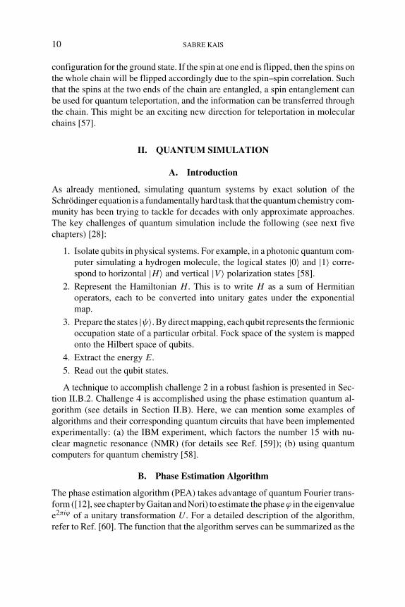
The generic quantum circuit for implementing PEA is shown in Fig. 2. Section 5.2of Ref. [12] presents a detailed account of how the circuit functions mathematicallyto yield the state |ϕ〉, which encodes the phase ϕ. Here we focus on its capabilityof finding the eigenvalues of a Hermitian matrix, which is of great importance inquantum chemistry where one often would like to find the energy spectrum of aHamiltonian.

Suppose we let U = eiAt0/2tfor some Hermitian matrix A, then eiAt0 |uj〉 =

eiλjt|uj〉, where λj and |uj〉 are the j-th eigenvalue and eigenvector of matrixA. Furthermore, we replace the initial state |u〉 of register b (Fig. 2) with anarbitrary vector |b〉 that has a decomposition in the basis of the eigenvectors of A:|b〉 = ∑n

j βj|uj〉. Then the major steps of the algorithm can be summarized as thefollowing.

1. Transform the t-qubit register C (Fig. 2) from |0〉⊗t to 1√2t

∑2t−1τ=0 |τ〉 state

by applying Hadamard transform on each qubit in register C.

2. Apply the U2kgates to the register b, where each U2k

gate is controlledby the (k − 1)th qubit of the register C from bottom. This series of con-trolled operations transforms the state of the two-register system from

1√2t

∑2t−1τ=0 |τ〉 ⊗ |b〉 to 1√

2t

∑2t−1τ=0 |τ〉 ∑n

j=1 eiλjτt/2tβj|uj〉.

3. Apply inverse Fourier transform FT† to the register C. Because every basisstate |τ〉 will be transformed to 1√

2t

∑2t−1k=0 e−2πiτk/2t |k〉 by FT†, the final

|0〉 H . . . •

†

.........

Reg. C FT|0〉 H • . . . |ϕ〉

|0〉 H • . . .

|0〉 H • . . .

Reg. b |u〉 / U20U21

U22 . . . U2t−1 |u〉

⎧⎪⎪⎪⎪⎪⎪⎪⎪⎨⎪⎪⎪⎪⎪⎪⎪⎪⎩

⎫⎪⎪⎪⎪⎪⎪⎪⎪⎬⎪⎪⎪⎪⎪⎪⎪⎪⎭

Figure 2. Schematic of the quantum circuit for phase estimation. The quantum wire with a “/”symbol represents a register of qubits as a whole. FT† represents inverse Fourier transform, whosecircuit is fairly standard ([12], see chapter by Gaitan and Nori).

12 SABRE KAIS

state of the PEA is proportional to∑2t−1

k=0∑n

j=1 ei(λjt0−2πk)τ/2tβj|k〉|uj〉.

Due to a well-known property of the exponential sum, in which sums ofthe form

∑N−1k=0 exp(2πik r

N) vanish unless r = 0 mod N, the values of k

are concentrated on those whose value is equal or close to t02π

λj . If we lett0 = 2π, the final state of system is

∑j βj|λj〉|uj〉 up to a normalization

constant.

In particular, if we prepare the initial state of register b to be one of matrixA’s eigenvector |ui〉, according to the procedure listed above, the final state ofthe system will become |λi〉|ui〉 up to a constant. Hence, for any |ui〉 that we canprepare, we can find the eigenvalue λj of A corresponding to |ui〉 using a quantumcomputer. Most importantly, it has been shown that [17] quantum computers areable to solve the eigenvalue problem significantly more efficiently than classicalcomputers.

2. Implementation of Unitary Transformation U

Phase estimation algorithm is often referred to as a black box algorithm becauseit assumes that the unitary transformation U and its arbitrary powers can beimplemented with basic quantum gates. However, in many cases U has a structurethat renders finding the exact decomposition U = U1U2...Um either impossible orvery difficult. Therefore, we need a robust method for finding approximate circuitdecompositions of unitary operators U with minimum cost and minimum fidelityerror.

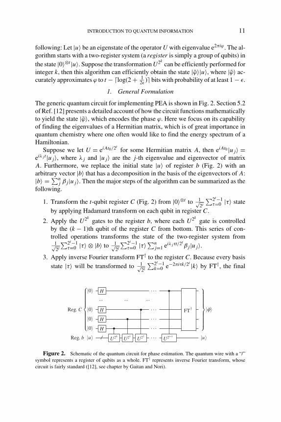
Inspired by the optimization nature of the circuit decomposition problem,Daskin and Kais [61,62] have developed an algorithm based on group leaderoptimization technique for finding a circuit decomposition U = U1U2...Um withminimum gate cost and fidelity error for a particular U. Hence, there are two fac-tors that need to be optimized within the optimization: the error and the cost ofthe circuit. The costs of a one-qubit gate and a control gate (two-qubit gate) aredefined as 1 and 2, respectively. Based on these two definitions, the costs of otherquantum gates can be deduced. In general, the minimization of the error to an ac-ceptable level is more important than the cost in order to get more reliable resultsin the optimization process. The circuit decompositions for U = eiAt presented inFig. 3b for the particular instance of A in Eq. (6) are found by the algorithm suchthat the error ||U ′ − U|| and the cost of U ′ are both minimized.

3. Group Leaders Optimization Algorithm

The group leaders optimization algorithm (GLOA) described in more detail inRefs [61,62] is a simple and effective global optimization algorithm that models theinfluence of leaders in social groups as an optimization tool. The algorithm startswith dividing the randomly generated solution population into several disjunctgroups and assigning for each group a leader (the best candidate solution inside


Reg. C

FT

01

e e

|0〉 H •†

|0〉 H •

|0〉

iAt0 /4 iAt0 /2

12√

2

∑j ( | 〉︸︷︷︸

λ1 =1

|u1j 〉 + |10〉︸︷︷︸λ2 =2

|u2j 〉)

Reg. b |0〉

|0〉

⎧⎨⎩⎧⎪⎪⎪⎪⎨⎪⎪⎪⎪⎩

⎫⎪⎪⎪⎪⎪⎪⎪⎪⎪⎪⎪⎬⎪⎪⎪⎪⎪⎪⎪⎪⎪⎪⎪⎭

(a)

X H • • Z H V †

• V Z Z V † Y X

T T V † Y • V S

(b)

Figure 3. Quantum circuit for estimating the eigenvalues of A, which is the 8 × 8 matrix shownin Eq. (6). (a) The overall circuit implementing the phase estimation algorithm. (b) Decomposition of

the gate eiAt04 in terms of basic gates.

the group). The algorithm basically is built on two parts: mutation and parametertransfer. In the mutation part, a candidate solution (a group member that is notleader) is mutated by using some part of its group leader, some random part, andsome part of this member itself. This mutation is formulated as

new member = r1 part of the member

∪ r2 part of its leader (5)

∪ r3 part of random

where r1, r2, and r3 determine the rates of the member, the group leader, andthe newly created random solution into the newly formed member, and they sumto 1. The values of these rates are assigned as r1 = 0.8 and r2 = r3 = 0.1. Themutation for the values of the all angles in a numerical string is done accordingto the arithmetic expression: anglenew = r1 × angleold + r2 × angleleader + r3 ×anglerandom, where angleold, the current value of an angle, is mutated: anglenew,the new value of the angle, is formed by combining a random value and thecorresponding leader of the group of the angle and the current value of the anglewith the coefficients r1, r2, and r3. The mutation for the rest of the elements inthe string means the replacement of its elements by the corresponding elementsof the leader and a newly generated random string with the rates r2 and r3. In thesecond part of the algorithm, these disjoint groups communicate with each other bytransferring some parts of their members. This step is called parameter transfer. In

14 SABRE KAIS

this process, some random part of a member is replaced with the equivalent part of arandom member from a different group. The amount of this communication processis limited with some parameter that is set to 4×maxgates

2 − 1, where the numerator isthe number of variables forming a numeric string in the optimization. During theoptimization, the replacement criterion between a newly formed member is and anexisting member is defined as follows: If a new member formed by a mutation ora parameter transfer operation gives less error-prone solution to the problem thanthe corresponding member, or they have the same error values but the cost of thenew member is less than this member, then the new member takes the former one’splace as a candidate solution; otherwise, the newly formed member is disregarded.

4. Numerical Example

In order to demonstrate how PEA finds the eigenvalues of a Hermitian matrix,here we present a numerical example. We choose A as a Hermitian matrixwith the degenerate eigenvalues λi = 1, 2 and corresponding eigenvectors|u11〉 = | + ++〉, |u12〉 = | + +−〉, |u13〉 = | + −+〉, |u14〉 = | − ++〉, |u21〉 =| − −−〉, |u22〉 = | − −+〉, |u23〉 = | − +−〉, |u24〉 = | + −−〉:

A =

⎛⎜⎜⎜⎜⎜⎜⎜⎜⎜⎜⎜⎜⎜⎝

1.5 −0.25 −0.25 0 −0.25 0 0 0.25

−0.25 1.5 0 −0.25 0 −0.25 0.25 0

−0.25 0 1.5 −0.25 0 0.25 −0.25 0

0 −0.25 −0.25 1.5 0.25 0 0 −0.25

−0.25 0 0 0.25 1.5 −0.25 −0.25 0

0 −0.25 0.25 0 −0.25 1.5 0 −0.25

0 0.25 −0.25 0 −0.25 0 1.5 −0.25

0.25 0 0 −0.25 0 −0.25 −0.25 1.5

⎞⎟⎟⎟⎟⎟⎟⎟⎟⎟⎟⎟⎟⎟⎠(6)

Here |+〉 = 1√2

(|0〉 + |1〉) and |−〉 = 1√2

(|0〉 − |1〉) represent the Hadamard

states. Furthermore, we let �b = (1, 0, 0, 0, 0, 0, 0, 0)T. Therefore, |b〉 = |000〉 =∑j βj|uj〉 and each βj = 1

2√

2. Figure 3 shows the circuit for solving the 8 × 8

linear system. The register C is first initialized with Walsh–Hadamard transfor-mation and then used as the control register for Hamiltonian simulation eiAt0

on the register B. The decomposition of the two-qubit Hamiltonian simulationoperators in terms of basic quantum circuits is achieved using group leaderoptimization algorithm [61,62]. The final state of system is

∑j βj|λj〉|uj〉 =

12√

2

∑4i=1(|01〉|u1i〉 + |10〉|u2i〉), which encodes both eigenvalues 1 (as |01〉) and

2 (as |10〉) in register C (Fig. 3).


5. Simulation of the Water Molecule

Wang et al.’s algorithm [19] can be used to obtain the energy spectrum of molecularsystems such as water molecule based on the multiconfigurational self-consistentfield (MCSCF) wave function. By using a MCSCF wave function as the initialguess, the excited states are accessible. The geometry used in the calculation isnear the equilibrium geometry (OH distance R = 1.8435a0 and the angle HOH =110.57◦). With a complete active space type MCSCF method for the excited-statesimulation, the CI space is composed of 18 CSFs, which requires the use of fivequbits to represent the wave function. The unitary operator for this Hamiltoniancan be formulated as

UH2O = eiτ(Emax−H)t (7)

where τ is given as

τ = 2π

Emax − Emin(8)

Emax and Emin are the expected maximum and minimum energies. The choice ofEmax and Emin must cover all the eigenvalues of the Hamiltonian to obtain thecorrect results. After finding the phase φj from the phase estimation algorithm,the corresponding final energy Ej is found from the following expression:

Ej = Emax − 2πφj

τ(9)

Because the eigenvalues of the Hamiltonian of the water molecule are between−80 ± ε and −84 ± ε (ε ≤ 0.1), taking Emax = 0 and Emin = −200 gives thefollowing:

U = e−i2πH

200 t (10)

Figure 4 shows the circuit diagram for this unitary operator generated by usingthe optimization algorithm and procedure as defined. The cost of the circuit is

Figure 4. The circuit design for the unitary propagator of the water molecule.

16 SABRE KAIS

TABLE IIIEnergy Eigenvalues of the Water Molecule

Phase Found Energy Exact Energy

0.4200 −84.0019 −84.00210.4200 −84.0019 −83.44920.4200 −84.0019 −83.02730.4200 −84.0019 −82.93740.4200 −84.0019 −82.77190.4200 −84.0019 −82.64960.4200 −84.0019 −82.52520.4200 −84.0019 −82.44670.4144 −82.8884 −82.39660.4144 −82.8884 −82.29570.4144 −82.8884 −82.06440.4144 −82.8884 −81.98720.4144 −82.8884 −81.85930.4144 −82.8884 −81.65270.4144 −82.8884 −81.45920.4144 −82.8884 −81.01190.4122 −82.4423 −80.90650.4122 −82.4423 −80.6703

44, which is found by summing up the cost of each gates in the circuit. Becausewe take Emax as zero, this deployment does not require any extra quantum gatefor the implementation within the phase estimation algorithm. The simulation ofthis circuit within the iterative PEA results in the phase and energy eigenvaluesgiven in Table III: The left two columns are, respectively, the computed phasesand the corresponding energies, while the rightmost column of the matrix is theeigenvalues of the Hamiltonian of the water molecule (for each value of the phase,the PEA is run 20 times).

III. ALGORITHM FOR SOLVING LINEAR SYSTEMS A�x = �b

A. General Formulation

The algorithm solves a problem where we are given a Hermitian s-sparse N×N

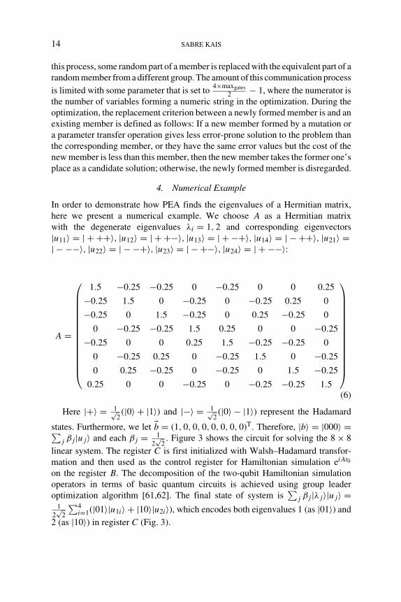
matrix A and a unit vector �b (Fig. 5). Suppose we would like to find �x such thatA�x = �b. The algorithm can be summarized as the following major steps [29]:

1. Represent the vector �b as a quantum state |b〉 = ∑Ni=1bi|i〉 stored in a quan-

tum register (termed register b). In a separate quantum register (termedregister C) of t qubits, initialize the qubits by transforming the register tostate |�〉C from |0〉 up to error ε�.


|0〉 Ry

√1− C2

λ2j|0〉 + C

λ j|1〉

|0〉 / W Rzz • • • Rzz W |0〉

|0〉 / W • e−iH0t0 eiH0t0 • W |0〉

|0〉 / W • FT† • • FT • W |0〉

|b〉 / e−iAt0 eiAt0 |b〉︸︷︷︸

Uncomputation

Figure 5. Generic quantum circuit for implementing the algorithm for solving linear systems ofequations. The registers from the bottom of the circuit diagram upwards are, respectively, registers b,C, m, and l. The qubit on the top of the figure represents the ancilla bit.

2. Apply the conditional Hamiltonian evolution∑T−1

τ=0 |τ〉〈τ|C ⊗ eiAτt0/T upto error εH.

3. Apply quantum inverse Fourier transform to the register C. Denote the basisstates after quantum Fourier transform as |k〉. At this stage in the superposi-tion state of both registers, the amplitudes of the basis states are concentratedon k values that approximately satisfy λk ≈ 2πk

t0, where λk is the kth eigen-

value of the matrix A.

4. Add an ancilla qubit and apply conditional rotation on it, controlledby the register C with |k〉 ≈ |λk〉. The rotation transforms the qubit to√

1 − C2

λ2j

|0〉 + Cλj

|1〉. This key step of the algorithm involves finding the

reciprocal of the eigenvalue λj quantum mechanically, which is not a trivialtask on its own. Now we assume that we have methods readily availableto find the reciprocal of the eigenvalues of matrix A and store them in aquantum register.

5. Uncompute the register b and C by applying Fourier transform on reg-ister C followed by the complex conjugates of same conditional Hamil-tonian evolution as in step 2 and Walsh–Hadamard transform as in thefirst step.

6. Measure the ancilla bit. If it returns 1, the register b of the system is inthe state

∑nj=1 βjλj

−1|uj〉 up to a normalization factor, which is equal to

the solution |x〉 of the linear system A�x = �b. Here |uj〉 represents the jtheigenvector of the matrix A and let |b〉 = ∑n

i=1 βj|uj〉.

18 SABRE KAIS

|0〉 Ry ( 2π2m−1 ) Ry ( π

2m−1 )

|0〉 H •

FT†× •

U†

|0〉 H • × •

|0〉

eiAt0 /4 eiAt0 /2|0〉

|0〉

(a)

X H • • Z H V †

• V Z Z V † Y X

T T V † Y • V S

(b)

Figure 6. Quantum circuit for solving A�x = �b with A8×8 being the matrix shown in Eq. (6).(a) The overall circuit. From bottom up are the two qubits for |b〉, zeroth qubit in register C for encodingthe eigenvalue, first qubit in register C for eigenvalue, and ancilla bit. U† represents uncomputation.

(b) Decomposition of the gate eiAt04 in terms of basic gates.

B. Numerical Example

For this example we choose A as the same Hermitian matrix as the one inEq. (6). Furthermore, we let �b = (1, 0, 0, 0, 0, 0, 0, 0)T. Therefore, |b〉 = |000〉 =∑

j βj|uj〉 and each βj = 12√

2. To compute the reciprocals of the eigenvalues, a

quantum swap gate is used (Fig. 6) to exchange the values of the zeroth and firstqubit. By exchanging the values of the qubits, one inverts an eigenvalue of A, say1 (encoded with |01〉), to |10〉, which represents 2 in binary form. In the same way,the eigenvalue 2 (|10〉) can be inverted to 1 |01〉.

Figure 6 shows the circuit for solving the 8 × 8 linear system. The register C isfirst initialized with Walsh–Hadamard transformation and then used as the controlregister for Hamiltonian simulation eiAt0 on the register B. The decomposition ofthe two-qubit Hamiltonian simulation operators in terms of basic quantum circuitsis achieved using group leader optimization algorithm [61,62].

The final state of system, conditioned on obtaining |1〉 in the ancilla bit, is1

2√

10(6|000〉 + |001〉 + |010〉 + |100〉 − |111〉), which is proportional to the exact

solution of the system �x = (0.75, 0.125, 0.125, 0, 0.125, 0, 0, −0.125)T.


IV. ADIABATIC QUANTUM COMPUTING

The model of adiabatic quantum computation (AQC) was initially suggested byFarhi, Goldstone, Gutman, and Sisper [63] for solving some classical optimizationproblems. Several years after the proposition of AQC, Aharonov, Dam, Kempe,Landau, Lloyd, and Regev [64] assessed its computational power and establishedthat the model of AQC is polynomially equivalent to the standard gate modelquantum computation. Nevertheless, this model provides a completely differentway of constructing quantum algorithms and reasoning about them. Therefore, itis seen as a promising approach for the discovery of substantially new quantumalgorithms.

Prior to the work by Aharonov et al. [64], it had been known that AQC canbe simulated by GMQC [65,66]. The equivalence between AQC and GMQC isthen proven by showing that standard quantum computation can be efficientlysimulated by adiabatic computation using 3-local Hamiltonians [64]. While theconstruction of three-particle Hamiltonians is sufficient for substantiating the the-oretical results, it is technologically difficult to realize. Hence, significant effortshave been devoted to simplifying the universal form of Hamiltonian to render itfeasible for physical implementation [64,67–70].

From the experimental perspective, current progress [71,72] in devices basedon superconducting flux qubits has demonstrated the capability to implementHamiltonian of the form ihiσ

zi + i�iσ

xi + i,jJijσ

zi σ

zj . However, this is not

sufficient for constructing a universal adiabatic quantum computer [71]. It isshown [68] that this Hamiltonian can be rendered universal by simply addinga tunable 2-local transverse σxσx coupling. Once tunable σxσx is available, allthe other 2-local interactions such as σzσx and σxσz can be reduced to sums ofsingle σx, σz spins and σxσx, σzσz couplings via a technique called Hamilto-nian gadgets. In Section IV.3, we will present a more detailed review of thissubject.

A. Hamiltonians of n-Particle Systems

In the standard GMQC, the state of n qubits evolves in discrete time steps byunitary operations. Physically, however, the evolution is continuous and is gov-erned by the Schrodinger equation: −i d

dt|ψ(t)〉 = H(t)|ψ(t)〉, where |ψ(t)〉 is the

state of n qubits at time t and H(t) is a Hermitian 2n × 2n matrix called theHamiltonian operating on the n-qubit system; it governs the dynamics of the sys-tem. The fact that it is Hermitian derives from the unitary property of the discretetime evolution of the quantum state from t1 to a later time t2. In some context,the eigenvalues of Hamiltonians are referred to as energy levels. The ground-state energy of a Hamiltonian is its lowest eigenvalue and the corresponding

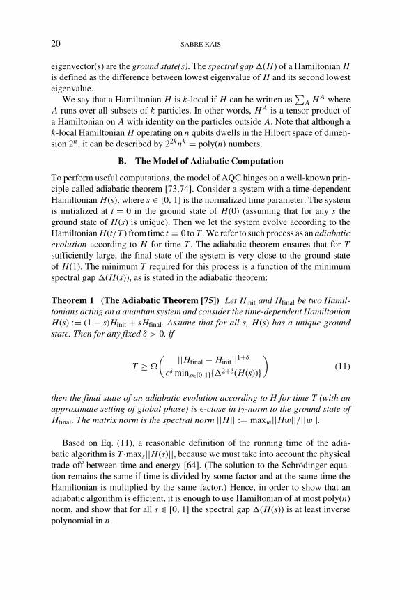
20 SABRE KAIS

eigenvector(s) are the ground state(s). The spectral gap �(H) of a Hamiltonian H

is defined as the difference between lowest eigenvalue of H and its second lowesteigenvalue.

We say that a Hamiltonian H is k-local if H can be written as∑

A HA whereA runs over all subsets of k particles. In other words, HA is a tensor product ofa Hamiltonian on A with identity on the particles outside A. Note that although ak-local Hamiltonian H operating on n qubits dwells in the Hilbert space of dimen-sion 2n, it can be described by 22knk = poly(n) numbers.

B. The Model of Adiabatic Computation

To perform useful computations, the model of AQC hinges on a well-known prin-ciple called adiabatic theorem [73,74]. Consider a system with a time-dependentHamiltonian H(s), where s ∈ [0, 1] is the normalized time parameter. The systemis initialized at t = 0 in the ground state of H(0) (assuming that for any s theground state of H(s) is unique). Then we let the system evolve according to theHamiltonian H(t/T ) from time t = 0 to T . We refer to such process as an adiabatic

evolution according to H for time T . The adiabatic theorem ensures that for T

sufficiently large, the final state of the system is very close to the ground stateof H(1). The minimum T required for this process is a function of the minimumspectral gap �(H(s)), as is stated in the adiabatic theorem:

Theorem 1 (The Adiabatic Theorem [75]) Let Hinit and Hfinal be two Hamil-tonians acting on a quantum system and consider the time-dependent HamiltonianH(s) := (1 − s)Hinit + sHfinal. Assume that for all s, H(s) has a unique groundstate. Then for any fixed δ > 0, if

T ≥ �

( ||Hfinal − Hinit||1+δ

εδ mins∈[0,1]{�2+δ(H(s))})

(11)

then the final state of an adiabatic evolution according to H for time T (with anapproximate setting of global phase) is ε-close in l2-norm to the ground state ofHfinal. The matrix norm is the spectral norm ||H || := maxw||Hw||/||w||.

Based on Eq. (11), a reasonable definition of the running time of the adia-batic algorithm is T ·maxs||H(s)||, because we must take into account the physicaltrade-off between time and energy [64]. (The solution to the Schrodinger equa-tion remains the same if time is divided by some factor and at the same time theHamiltonian is multiplied by the same factor.) Hence, in order to show that anadiabatic algorithm is efficient, it is enough to use Hamiltonian of at most poly(n)norm, and show that for all s ∈ [0, 1] the spectral gap �(H(s)) is at least inversepolynomial in n.


C. Hamiltonian Gadgets

A perturbation gadget or simply a gadget Hamiltonian refers to a Hamiltonian con-struction invented by Kempe, Kitaev, and Regev [67] first used to approximatethe ground states of k-body Hamiltonians using the ground states of two-bodyHamiltonians. Gadgets have been used and/or extended by several authors includ-ing Oliveira and Terhal [76–79]. Recent results have been reviewed in the articleby Wolf [80]. Gadgets have a range of applications in quantum information theory,many-body physics, and are mathematically interesting to study in their own right.They have recently come to occupy a central role in the solution of several impor-tant and long-standing problems in quantum information theory. Kempe, Kitaev,and Regev [81] introduced these powerful tools to show that finding the groundstate of a 2-local system (i.e., a system with at most two-body interactions) is in thesame complexity class QMA as finding the ground-state energy of a system withk-local interactions. This was done by introducing a gadget that reduced 3-local to2-local interactions. Oliveira and Terhal [76] exploited the use of gadgets to ma-nipulate Hamiltonians acting on a 2D lattice. The work in [76,81] was instrumentalin finding simple spin models with a QMA-complete ground-state energy problem[78]. Aside from complexity theory, Hamiltonian gadget constructions have im-portant application in the area of adiabatic quantum computation [76,77,81]. Theapplication of gadgets extends well beyond the scope mentioned here.

V. TOPOLOGICAL QUANTUM COMPUTING

Topological quantum computation seeks to exploit the emergent properties ofmany-particle systems to encode and manipulate quantum information in a man-ner that is resistant to error. This scheme of quantum computing supports the gatemodel of quantum computation. Quantum information is stored in states with mul-tiple quasi particles called anyons, which have a topological degeneracy and aredefined in the next section. The unitary gate operations that are necessary for quan-tum computation are carried out by performing braiding operation on the anyonsand then measuring the multiquasipartite states. The fault tolerance of a topologi-cal quantum computer arises from the nonlocal encoding of the quasipartite states,which render them immune to errors by local perturbations.

A. Anyons

Two-dimensional systems are qualitatively different [82] from three-dimensionalones. In three-dimensional space, only two symmetries are possible: the time-dependent wave function of bosons is symmetric under exchange of particles whilethat of fermions is antisymmetric. However, in a two-dimensional case when twoparticles are interchanged twice in a clockwise manner, their trajectory in space-time involves a nontrivial winding, and the system does not necessarily come back

22 SABRE KAIS

to the same state. The first realization of this topological difference dates back tothe 1980s [83,84] and it leads to a difference in the possible quantum mechanicalproperties for quantum systems when particles are confined to two dimensions.Suppose we have two identical particles in two dimensions. When one particleis exchanged in a counterclockwise manner with the other, the wave functionψ(�r1, �r2) can change by an arbitrary phase: ψ(�r1, �r2) → eiφψ(�r1, �r2). The specialcases where φ = 0, π correspond to bosons and fermions, respectively. Particleswith other values of φ are called anyons [85].

B. Non-Abelian Braid Groups

In three-dimensional space, suppose we have N indistinguishable particles and weconsider all possible trajectories in the space-time (or four-dimensional worldli-ness), which take these N particles from initial positions �r1, �r2, . . . , �rN at time t0to final positions �r′

1, �r′2, . . . , �r′

N at time tf . Then the different trajectories fall intotopological classes corresponding to the elements of the permutation group SN ,with each element specifying how the initial positions are permuted to obtain thefinal positions. The way the permutation group acts on the states of the systemdefines the quantum evolution of such a system. Fermions and bosons correspondto the only two one-dimensional irreducible representations of the permutationgroup of N identical particles.

In two-dimensional space, the topological classes of the trajectories that takethese particles from initial positions �r1, �r2, . . . , �rN at time t0 to final positions�r′

1, �r′2, . . . , �r′

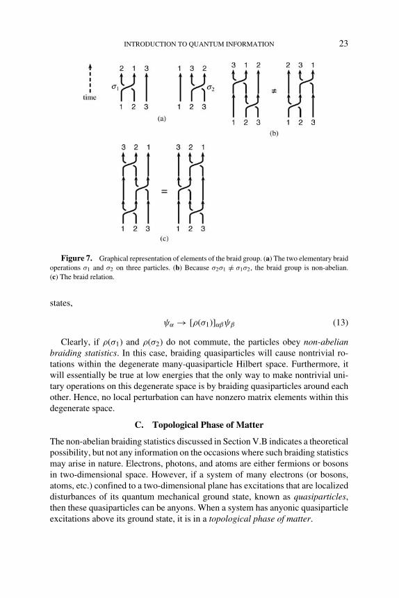
N at time tf are in one-to-one correspondence with the elements ofthe braid group BN . An element of the braid group can be visualized by consider-ing the trajectories of particles as world lines in (2 + 1)-dimensional space-timeoriginating at initial positions and terminating at final positions (Fig. 7a). Themultiplication of two elements of the braid group is the successive execution ofthe corresponding trajectories (i.e., the vertical stacking of the two drawings). Asshown in Fig. 7b, the order in which they are multiplied is important becausethe group is non-abelian, which means multiplication is not commutative. Alge-braically, the braid group can be represented in terms of elementary braid oper-ations, or generators σi, with 1 ≤ i ≤ N − 1. σi is a counterclockwise exchangeof the ith and (i + 1)th particles. σ−1

i is therefore a clockwise exchange of the ithand the (i + 1)th particles. The σi’s satisfy the defining relations (Fig. 7c)

σiσj = σjσi if |i − j| ≥ 2

σiσi+1σi = σi+1σiσi+1 if 1 ≤ i ≤ n − 1(12)

The richness of the braid group is that it supports quantum computation. Todefine the quantum evolution of a system, we specify how the braid group acts onthe states of the system. An element of the braid group, say σ1, which exchangesparticles 1 and 2, is represented by a g × g unitary matrix ρ(σ1) acting on these


Figure 7. Graphical representation of elements of the braid group. (a) The two elementary braidoperations σ1 and σ2 on three particles. (b) Because σ2σ1 /= σ1σ2, the braid group is non-abelian.(c) The braid relation.

states,

ψα → [ρ(σ1)]αβψβ (13)

Clearly, if ρ(σ1) and ρ(σ2) do not commute, the particles obey non-abelianbraiding statistics. In this case, braiding quasiparticles will cause nontrivial ro-tations within the degenerate many-quasiparticle Hilbert space. Furthermore, itwill essentially be true at low energies that the only way to make nontrivial uni-tary operations on this degenerate space is by braiding quasiparticles around eachother. Hence, no local perturbation can have nonzero matrix elements within thisdegenerate space.

C. Topological Phase of Matter

The non-abelian braiding statistics discussed in Section V.B indicates a theoreticalpossibility, but not any information on the occasions where such braiding statisticsmay arise in nature. Electrons, photons, and atoms are either fermions or bosonsin two-dimensional space. However, if a system of many electrons (or bosons,atoms, etc.) confined to a two-dimensional plane has excitations that are localizeddisturbances of its quantum mechanical ground state, known as quasiparticles,then these quasiparticles can be anyons. When a system has anyonic quasiparticleexcitations above its ground state, it is in a topological phase of matter.

24 SABRE KAIS

Topological quantum computation is predicated on the existence in nature oftopological phases of matter. Topological phases can be defined as (i) degenerateground states, (ii) gap to local excitations, (iii) abelian or non-abelian quasiparti-cle excitations. Because these topological phases occur in many-particle physicalsystems, field theory techniques are often used to study these states. Hence, thedefinition of topological phase may be stated more compactly by simply sayingthat a system is in a topological phase if its low-energy effective field theory is atopological quantum field theory (TQFT), that is, a field theory whose correlationfunctions are invariant under diffeomorphisms. For a more detailed account ofrecent development in TQFT and topological materials, see the work of Vala andcoworkers (see chapter by Watts et al.).

D. Quantum Computation Using Anyons

The braiding operation ρ(σi) defined in Eq. (13) can be cascaded to perform quan-tum gate operation. For example, Georgiev [86] showed that a CNOT gate can beexecuted on a six-quasiparticle system (for details refer to Ref. [86] or a compre-hensive review in Ref. [87]):

ρ(σ−13 σ4σ3σ1σ5σ4σ

−13 ) =

⎛⎜⎜⎜⎝

1 0 0 0

0 1 0 0

0 0 0 1

0 0 1 0

⎞⎟⎟⎟⎠ (14)

In the construction by Georgiev, quasiparticles 1 and 2 are combined to be qubit1 via an operation called fusion. Similarly, quasiparticles 5 and 6 are combined tobe qubit 2. We will not be concerned about the details of fusion in this introduction.Interested readers can refer to Ref. [87], Section II for more information. Apartfrom CNOT, single-qubit gates are also needed for universal quantum computation.One way to implement those single-qubit gates is to use nontopological operations.More details on this topic can be found in Ref. [88].

VI. ENTANGLEMENT

The concept of entanglement can be defined based on a postulate of quantummechanics. The postulate states that the state space of a composite physical systemis the tensor product of the states of the component physical systems. Moreover,if we have systems numbered 1 through n, and the system number i is preparedin the state |ψi〉, then the joint state of the total system is |ψ〉 = |ψ1〉 ⊗ |ψ2〉⊗ . . . ⊗ |ψn〉. However, in some cases |ψ〉 cannot be written in the form of atensor product of states of individual component systems. For example, the well-known Bell state or EPR pair (named after Einstein, Podolsky, and Rosen for their


initial proposition of this state [89]) |ψ〉 = 1√2

(|00〉 + |11〉) cannot be written inform of |a〉 ⊗ |b〉. States such as this are called entangled states. The opposite caseis a disentangled state.

In fact, entanglement in a state is a physical property that should be quanti-fied mathematically, which leads to a question of defining a proper expressionfor calculating entanglement. Various definitions have been proposed to mathe-matically quantify entanglement (for a detailed review see Refs. [5,90]). One ofthe most commonly used measurement for pairwise entanglement is concurrence

C(ρ), where ρ is the density matrix of the state. This definition was proposed byWootters [91]. The procedure for calculating concurrence is the following (formore examples illustrating how to calculate concurrence in detail, refer to Refs.[5,92,93]):

• Construct the density matrix ρ.• Construct the flipped density matrix, ρ = (σy ⊗ σy)ρ∗(σy ⊗ σy).• Construct the product matrix ρρ.• Find eigenvalues λ1, λ2, λ3, and λ4 of ρρ.• Calculate concurrence from square roots of eigenvalues via

C = max(0,

√λ1 − √

λ2 − √λ3 − √

λ4)

(15)

Physically, C = 0 means no entanglement in the two-qubit state ρ and C = 1represents maximum entanglement. Therefore, any state ρ with C(ρ) > 0 is anentangled state. An entangled state has many surprising properties. For example,if one measures the first qubit of the EPR pair, two possible results are obtained:0 with probability 1/2, where postmeasurement the state becomes |00〉, and 1with probability 1/2, where postmeasurement the state becomes |11〉. Hence, ameasurement of the second qubit always gives the same result as that of the firstqubit. The measurement outcomes on the two qubits are therefore correlated insome sense. After the initial proposition by EPR, John Bell [94] proved that themeasurement correlation in the EPR pair is stronger than could ever exist betweenclassical systems. These results (refer to Ref. [12], Section 2.6 for details) werethe first indication that laws of quantum mechanics support computation beyondwhat is possible in the classical world.

Entanglement has also been used to measure interaction and correlation inquantum systems. In quantum chemistry, the correlation energy is defined as thedifference between the Hartree–Fock limit energy and the exact solution of thenonrelativistic Schrodinger equation. Other measures of electron correlation exist,such as the statistical correlation coefficients [95] and, more recently, the Shannonentropy [96]. Electron correlations strongly influence many atomic, molecular, andsolid properties. Recovering the correlation energy for large systems remains one

26 SABRE KAIS

of the most challenging problems in quantum chemistry. We have used the entan-glement as a measure of the electron–electron correlation [5,92,93] and show thatthe configuration interaction (CI) wave function violates the Bell inequality [97].Entanglement is directly observable via macroscopic observable called entangle-ment witnesses [98]. Of particular interest is how entanglement plays a role inconical intersections and Landau–Zener tunneling and whether ideas from quan-tum information such as teleportation can be used to understand spin correlationsin molecules [99].

Since the original proposal by DeMille [100], arrays of ultracold polarmolecules have been counted among the most promising platforms for the im-plementation of a quantum computer [101–103]. The qubit of such an array isrealized by a single dipolar molecule entangled via its dipole–dipole interactionwith the rest of the array’s molecules. Polar molecule arrays appear as scalable to alarge number of qubits as neutral atom arrays do, but the dipole–dipole interactionfurnished by polar molecules offers a faster entanglement, one resembling thatmediated by the Coulomb interaction for ions. At the same time, cold and trappedpolar molecules exhibit similar coherence times as those encountered for trappedatoms or ions. The first proposed complete scheme for quantum computing withpolar molecules was based on an ensemble of ultracold polar molecules trapped ina one-dimensional optical lattice, combined with an inhomogeneous electrostaticfield. Such qubits are individually addressable, thanks to the Stark effect, which isdifferent for each qubit in the inhomogeneous electric field. In collaboration withWei, Friedrich, and Herschbach [93], we have evaluated entanglement of the pen-dular qubit states for two linear dipoles, characterized by pairwise concurrence, asa function of the molecular dipole moment and rotational constant, strengths of theexternal field and the dipole–dipole coupling, and ambient temperature. We alsoevaluated a key frequency shift, δω, produced by the dipole–dipole interaction.Under conditions envisioned for the proposed quantum computers, both the con-currence and δω become very small for the ground eigenstate. In principle, suchweak entanglement can be sufficient for operation of logic gates, provided the res-olution is high enough to detect the δω shift unambiguously. In practice, however,for many candidate polar molecules it appears a challenging task to attain adequateresolution. Overcoming this challenge, small δω shift, will be a major contributionto implementation of the DeMille proposal. Moreover, it will open the door fordesigning quantum logical gate: one-qubit gate (such as the rotational X, Y, Zgates and the Hadamard gate) and two-qubit quantum gates (such as the CNOTgate) for molecular dipole arrays. The operation of a quantum gate [104] such asCNOT requires that manipulation of one qubit (target) depends on the state of an-other qubit (control). This might be characterized by the shift in the frequency fortransition between the target qubit states when the control qubit state is changed.The shift must be kept smaller than the differences required to distinguish amongaddresses of qubit sites. In order to implement the requisite quantum gates, one


might use algorithmic schemes of quantum control theory for molecular quantumgates developed by de Vivie-Riedle and coworkers [105–107], Herschel Rabitz,and others [108–112].

Recent experimental discoveries in various phenomena have provided furtherevidence of the existence of entanglement in nature. For example, photosynthesisis one of the most common phenomena in nature. Recent experimental results showthat long-lived quantum entanglement are present in various photosynthetic com-plexes [113–115]. One such protein complex, the Fenna–Matthews–Olson (FMO)complex from green sulfur bacteria [116,117], has attracted considerable exper-imental and theoretical attention due to its intermediate role in energy transport.The FMO complex plays the role of a molecular wire, transferring the excita-tion energy from the light-harvesting complex (LHC) to the reaction center (RC)[118–120]. Long-lasting quantum beating over a timescale of hundreds of fem-toseconds has been observed [121,122]. The theoretical framework for modelingthis phenomenon has also been explored intensively by many authors [123–145].

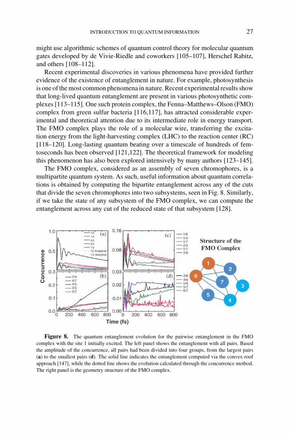
The FMO complex, considered as an assembly of seven chromophores, is amultipartite quantum system. As such, useful information about quantum correla-tions is obtained by computing the bipartite entanglement across any of the cutsthat divide the seven chromophores into two subsystems, seen in Fig. 8. Similarly,if we take the state of any subsystem of the FMO complex, we can compute theentanglement across any cut of the reduced state of that subsystem [128].

Figure 8. The quantum entanglement evolution for the pairwise entanglement in the FMOcomplex with the site 1 initially excited. The left panel shows the entanglement with all pairs. Basedthe amplitude of the concurrence, all pairs had been divided into four groups, from the largest pairs(a) to the smallest pairs (d). The solid line indicates the entanglement computed via the convex roofapproach [147], while the dotted line shows the evolution calculated through the concurrence method.The right panel is the geometry structure of the FMO complex.

28 SABRE KAIS

Pairwise entanglement plays the dominant entanglement role in the FMO com-plex. Because of the saturation of the monogamy bounds, the entanglement of anychromophore with any subset of the other chromophores is completely determinedby the set of pairwise entanglements. For the simulations in which site 1 is initiallyexcited, the dominant pair is sites 1 and 2, while in the cases where 6 is initially ex-cited sites 5 and 6 are most entangled. This indicates that entanglement is dominantin the early stages of exciton transport, when the exciton is initially delocalizedaway from the injection site. In addition, we observe that the entanglement mainlyhappens among the sites involved in the pathway. For the site 1 initially excitedcase, the entanglement of sites 5, 6, and 7 is relatively small compared with thedomain pairs.

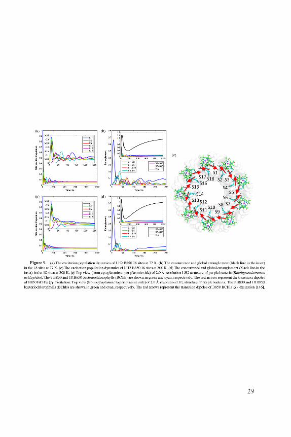
Although the final state is the same for both initial conditions, the role of sites3 and 4 during the time evolution is different. For the initial condition where site1 is excited, the entanglement is transferred to site 3 and then from site 3 to site4. While for the site 6 initially excited case, sites 4 and 5 first become entangledwith site 6 and then sites 3 and 4 become entangled. This is due to the fact that site3 has strong coupling with sites 1 and 2, while site 4 is coupled more strongly tosites 5, 6, and 7. The initial condition plays an important role in the entanglementevolution, the entanglement decays faster for the cases where site 6 is initiallyexcited compared with cases where the site 1 is initially excited. Increasing thetemperature unsurprisingly reduces the amplitude of the entanglement and alsodecreases the time for the system to go to thermal equilibrium. Recently [146],using the same formalism, we have calculated the pairwise entanglement for theLH2 complex, as seen in Fig. 9.

Apart from photosynthesis, other intriguing possibilities that living systemsmay use nontrivial quantum effects to optimize some tasks have been raised,such as natural selection [148] and magnetoreception in birds [149]. In particular,magnetoreception refers to the ability to sense characteristics of the surroundingmagnetic field. There are several mechanisms by which this sense may operate[150]. In certain species, the evidence supports a mechanism called radical pair

(RP). This process involves the quantum evolution of a spatially separated pair ofelectron spins [151,152]. The basic idea of the RP model is that there are molecularstructures in the bird’s eye that can each absorb an optical photon and give rise to aspatially separated electron pair in a singlet spin state. Because of the different localenvironments of the two electron spins, a singlet–triplet evolution occurs. This evo-lution depends on the inclination of the molecule with respect to Earth’s magneticfield. Recombination occurs from either the singlet or triplet state, leading to differ-ent chemical products. The concentration of these products constitutes a chemicalsignal correlated to Earth’s field orientation. Such a model is supported by severalresults from the field of spin chemistry [153–156]. An artificial chemical compassoperating according to this principle has been demonstrated experimentally [157],and the presence of entanglement has been examined by a theoretical study [158].

30 SABRE KAIS

Not only is entanglement found in nature, but it also plays a central role inthe internal working of a quantum computer. Consider a system of two qubits 1and 2. Initially, qubit 1 is in the state |ψ1〉 = |+〉 = 1√

2(|0〉 + |1〉) and qubit 2 is

in the state |ψ2〉 = |0〉. Hence, the initial state of the system can be written as|�0〉 = |ψ1〉 ⊗ |ψ2〉 = 1√

2(|00〉 + |10〉). Now apply a CNOT on qubits 1 and 2

with qubit 1 as the control and qubit 2 as the target. By definition of CNOT gate inSection I.A, the resulting state is 1√

2(|00〉 + |11〉), which is the EPR pair. Note that

the two qubits are initially disentangled. It is due to the CNOT operation that thetwo qubits are in an entangled state. Mathematically UCNOT cannot be representedas A ⊗ B, because if it could, (A ⊗ B)(|ψ1〉 ⊗ |ψ2〉) = (A|ψ1〉 ⊗ B|ψ2〉) wouldstill yield a disentangled state.

CNOT gate is indispensable for any set of universal quantum gates. Therefore,if a particular computation process involves n qubits that are initially disentangled,most likely all the n qubits need to be entangled at some point of the computation.This poses a great challenge for experimentalists because in order to keep a largenumber of qubits entangled for an extended period of time, a major issue needs tobe resolved—decoherence.

VII. DECOHERENCE

So far in our discussion of qubits, gates, and algorithms we assume the idealsituation where the quantum computer is perfectly isolated when performing com-putation. However, in reality this is not feasible because there is always interactionbetween the quantum computer and its environment, and if one would like to readany information from the final state of the quantum computer, the system has to beopen to measurements at least at that point. Therefore, a quantum computer is infact constantly subject to environmental noise, which corrupts its desired evolution.Such unwanted interaction between the quantum computer and its environment iscalled decoherence, or quantum noise.

Decoherence has been a main obstacle to building a quantum computing device.Over the years, various ways of suppressing quantum decoherence have beenexplored [159]. The three main error correction strategies for counteracting theerrors induced by the coupling with the environment include the following (seechapter by Lidar):

• Quantum error correction codes (QECCs), which uses redundancy and anactive measurement and recovery scheme to correct errors that occur duringa computation [160–164]

• Decoherence-free subspaces (DFSs) and noiseless subsystems, which relyon symmetric system–bath interactions to end encodings that are immune todecoherence effects [165–170]


• Dynamical decoupling, or “bang-bang” (BB) operations, which are strongand fast pulses that suppress errors by averaging them away [171–175]

Of these error correction techniques, QECCs require at least a five physicalqubit to one logical qubit encoding [163] (neglecting ancillas required for fault-tolerant recovery) in order to correct a general single-qubit error [162]. DFSs alsorequire extra qubits and are most effective for collective errors, or errors wheremultiple qubits are coupled to the same bath mode [170]. The minimal encodingfor a single qubit undergoing collective decoherence is three physical qubits toone logical qubit [168]. The BB control method requires a complete set of pulsesto be implemented within the correlation time of the bath [171]. However, it doesnot necessarily require extra qubits.

Although the ambitious technological quest for a quantum computer has facedvarious challenges, as of now no fundamental physical principle has been foundto prevent a scalable quantum computer from being built. Therefore, if we keepthis prospect, one day we will be able to maintain entanglement and overcomedecoherence to a degree such that scalable quantum computers become reality.

VIII. MAJOR CHALLENGES AND OPPORTUNITIES

Many of the researchers in the quantum information field have recognized quan-tum chemistry as one of the early applications of quantum computing devices. Thisrecognition is reflected in the document “A Federal Vision for Quantum Informa-tion Science,” published by the Office of Science and Technology Policy (OSTP) ofthe White House. As mentioned earlier, the development and use of quantum com-puters for chemical applications has potential for revolutionary impact on the waycomputing is done in the future. Major challenges and opportunities are abundant;examples include developing and implementing quantum algorithms for solvingchemical problems thought to be intractable for classical computers. To performsuch quantum calculations, it will be necessary to overcome many challenges inexperimental quantum simulation. New methods to suppress errors due to faultycontrols and noisy environments will be required. These new techniques wouldbecome part of a quantum compiler that translates complex chemical problems intoquantum algorithms. Other challenges include the role of quantum entanglement,coherence, and superposition in photosynthesis and complex chemical reactions.

Many exciting opportunities for science and innovation can be found in thisnew area of quantum information for chemistry including topological quantumcomputing (see chapter by Watts et al.), improving classical quantum chemistrymethods (see chapter by Kinder et al.), quantum error corrections (see chapterby Lidar), quantum annealing with D-Wave machine [176], quantum algorithmsfor solving linear systems of equations, and entanglement in complex biologicalsystems (see chapter by Mazziotti and Skochdopole). With its 128 qubits, the

32 SABRE KAIS

D-Wave computer at USC (the DW-1) is the largest quantum information processorbuilt to date. This computer will grow to 512 qubits (the chip currently beingcalibrated and tested by D-Wave Inc. (D. A. Lidar, private communication, USC,2012)), at which point we may be on the cusp of demonstrating, for the first timein history, a quantum speedup over classical computation. Various applicationsof DW-1 in chemistry include, for example, the applications in cheminformatics(both in solar materials and in drug design) and in lattice protein folding, and thesolution of the Poisson equation and its applications in several fields. While theDW-1 is not a universal quantum computer, it is designed to solve an importantand broad class of optimization problems—essentially any problem that can bemapped to the NP-hard problem of finding the ground state of a general planarIsing model in a magnetic field.

This chapter focused mainly on the theoretical aspects of quantum informationand computation for quantum chemistry and represents a partial overview of theongoing research in this field. However, a number of experimental groups areworking to explore quantum information and computation in chemistry: using iontrap (see chapter by Merrill and Brown) [177], NMR (see chapter by Criger etal.) [178–182], trapped molecules in optical lattice (see chapter by Cote) [183],molecular states (see chapter by Gollub et al.) [184,185], and optical quantumcomputing platforms (see chapter by Ma et al.) [186,187], to name just a few. Forexample, Brown and coworkers [177] proposed a method for laser cooling of theAlH+ and BH molecules. One challenge of laser cooling molecules is the accuratedetermination of spectral lines to 10−5 cm−1. In their work, the authors showthat the lines can be accurately determined using quantum logic spectroscopy andsympathetic heating spectroscopy techniques, which were derived from quantuminformation experiments. Also, Dorner and coworkers [188] perform the simplestdouble-slit experiment to understand the role of interference and entanglement inthe double photoionization of H2 molecule. Moreover, many more areas of overlaphave not been reviewed in detail here, notably coherent quantum control of atomsand molecules. However, we hope this chapter provides a useful introduction to thecurrent research directions in quantum information and computation for chemistry.

Finally, I would like to end this chapter by quoting Jonathan Dowling [189]:“We are currently in the midst of a second quantum revolution. The first one gaveus new rules that govern physical reality. The second one will take these rules anduse them to develop new technologies. Today there is a large ongoing internationaleffort to build a quantum computer in a wide range of different physical systems.Suppose we build one, can chemistry benefit from such a computer? The answeris a resounding YES!”

Acknowledgments

I would like thank Birgitta Whaley for her critical reading of this chapter and mystudents Yudong Cao, Anmer Daskin, Jing Zhu, Yeh Shuhao, Qi Wei, Qing Xu,


and Ross Hoehn for their major contributions to the materials discussed in thischapter. Also, I benefited from collaborating and discussing different aspects ofthis chapter with my colleagues: Alan Aspuru-Guzik, Daniel Lidar, Ken Brown,Peter Love, V. Ara Apkarian, Anargyros Papageorgiou, Bretislav Friedrich, UriPeskin, Gehad Sadiek, and Dudley Herschbach.

This work is supported by NSF Center for Quantum Information for Chemistry(QIQC), http://web.ics.purdue.edu/ kais/qc/ (award number CHE-1037992).

REFERENCES

1. M. Sarovar, A. Ishizaki, G. R. Fleming, and K. B. Whaley, Nat. Phys. 6, 462 (2010).

2. K. B. Whaley, Nat. Phys. 8, 10 (2012).

3. I. Kassal, J. D. Whitfield, A. Perdomo-Ortiz, M. Yung, and A. Aspuru-Guzik, Annu. Rev. Phys.Chem. 62, 185 (2011).

4. W. J. Kuo and D. A. Lidar, Phys. Rev. A 84, 042329 (2011).

5. S. Kais, in Reduced-Density-Matrix Mechanics: With Application to Many-Electron Atoms andMolecules, Advances in Chemical Physics, Vol. 134, D. A. Mazziotti, ed., Wiley-Interscience,2007, p. 493.

6. S. Lloyd, Science 319, 1209 (2008).

7. J. Elbaz, O. Lioubashevski, F. Wang, F. Remacle, R. D. Levine, and I. Willner. Nat. Nanotechnol.5, 417–422 (2011).

8. R. P. Feynmann, Int. J. Theor. Phys. 21(6–7), 467–488 (2008).

9. D. Deutsch, Proc. R. Soc. Lond. 400, 97–117 (1985).

10. P. Benioff, J. Stat. Phys. 29, 515–546 (1982).

11. C. H. Bennett and G. Brassard, Proceedings of IEEE International Conference on ComputersSystems and Signal Processing, 1984, pp. 175–179.

12. M. A. Nielsen and I. L. Chuang, Quantum Computation and Quantum Information, CambridgeUniversity Press, Cambridge, UK, 2000.

13. P. W. Shor, in Proceedings of the 35th Annual Symposium on Foundations of Computer Science,S. Goldwasser, ed., IEEE Computer Society Press, New York, 1994, pp. 124–134.

14. S. Lloyd, Science 273, 1073–1078 (1996).

15. D. Abrams and S. Lloyd, Phys. Rev. Lett. 83(24), 5162–5165 (1999).

16. D. Abrams and S. Lloyd, Phys. Rev. Lett. 79(13), 2586–2589 (1997).

17. A. Papageorgiou, I. Petras, J. F. Traub, and C. Zhang, Mathematics of Computation 82, 2293–2304(2013).

18. A. Papageorgiou and C. Zhang, arXiv:1005.1318v3 (2010).

19. H. Wang, S. Kais, A. Aspuru-Guzik, and M. R. Hoffmann, Phys. Chem. Chem. Phys. 10, 5388–5393 (2008).

20. A. Aspuru-Guzik, A. D. Dutoi, P. J. Love, and M. Head-Gordon, Science 379(5741), 1704–1707(2005).

21. D. Lidar and H. Wang, Phys. Rev. E 59, 2429 (1999).

22. H. Wang, S. Ashhab, and F. Nori, Phys. Rev. A 85, 062304 (2012).

23. J. Q. You and F. Nori, Nature 474, 589 (2011).

http://web.ics.purdue.edu/~kais/qc/

34 SABRE KAIS

24. J. Q. You and F. Nori, Phys. Today 58(11), 42–47 (2005).

25. I. Buluta and F. Nori, Science 326, 108 (2009).

26. J. P. Dowling, Nature 439, 919 (2006).

27. L. Veis and J. Pittner, J. Chem. Phys. 133, 194106 (2010).

28. L. Veis, J. Visnak, T. Fleig, S. Knecht, T. Saue, L. Visscher, and J. Pittner, arXiv:1111.3490v1(2011).

29. A. W. Harrow, A. Hassidim, and S. Lloyd, Phys. Rev. Lett. 15, 150502 (2009).

30. A. Klappenecker and M. Roetteler, arXiv:quant-ph/0111038 (2001).

31. P. A. M. Dirac, Proc. Roy. Soc. 123, 714 (1929).

32. S. Aaronson, Nat. Phys. 5, 707 (2009).

33. N. Schuch and F. Verstraete, Nat. Phys. 5, 732 (2009).

34. A. Szabo and N. S. Ostlund, Modern Quantum Chemistry—Introduction to Advanced ElectronicStructure Theory, Dover Publications Inc., Mineola, NY, 1982.

35. R. G. Parr and W. Yang, Density-Functional Theory of Atoms and Molecules, Oxford SciencePublications, New York, 1989.

36. D. A. Mazziotti, Adv. Chem. Phys. 134, 1 (2007).

37. I. Iachello and R. D. Levine, Algebraic Theory of Molecules, Oxford Univesity Press, 1995.

38. M. P. Nightingale and C. J. Umrigar, Quantum Monte Carlo Methods in Physics and Chemistry,NATO Science Series, Vol. 525, Springer, 1998.

39. D. R. Herschbach, J. Avery, and O. Goscinski, Dimensional Scaling in Chemical Physics, KluwerAcademic Publishers, Dordrecht, The Netherlands, 1993.

40. H. Dachsel, R. J. Harrison, and D. A. Dixon, J. Phys. Chem. A 103, 152–155 (1999).

41. D. P. DiVincenzo, arXiv:quant–ph/0002077 (2000).

42. T. D. Ladd, F. Jelezko, R. Laflamme, Y. Nakamura, C. Monroe, and J. L. O’Brien, Nature 464(4),45 (2010).

43. R. L. de Visser and M. Blaauboer, Phys. Rev. Lett. 96, 246801 (2006).

44. P. Jian-Wei, B. Dik, D. Matthew, W. Harald, and A. Zeilinge, Nature 403, 515 (2000).

45. P. Chen, C. Piermarocchi, and L. J. Sham, Phys. Rev. Lett. 87, 067401 (2001).

46. F. de Pasquale, G. Giorgi, and S. Paganelli, Phys. Rev. Lett. 93, 12052 (2004).

47. J. H. Reina and N. F. Johnson, Phys. Rev. A 63, 012303 (2000).

48. D. Bouwmeester, J. Pan, K. Mattle, M. Eibl, H. Weinfurter, and A. Zeilinger, Nature 390, 575(1997).

49. C. W. J. Beenakker and M. Kindermann, Phys. Rev. Lett. 95, 056801 (2004).

50. M. D. Barrett, J. Chiaverinl, and T. Schaetz, et al., Nature 429, 737 (2004).

51. M. Riebe, et al., Nature 429, 734 (2004).

52. H. Wang and S. Kais, Chem. Phys. Lett. 421, 338 (2006).

53. C. H. Bennett, G. Brassard, C. Crepeau, R. Jozsa, A. Peres, and W. Wootters, Phys. Rev. Lett.70, 1895 (1993).

54. C. P. Williams. Explorations in Quantum Computing, 2nd ed., Springer, 2011, p. 483.

55. R. Ursin, T. Jennewein, M. Aspelmeyer, R. Kaltenbaek, M. Lindenthal, P. Walther, andA. Zeilinge, Nature 430, 849 (2004).

56. R. Ursin, F. Tiefenbacher, T. Schmitt-Manderbach, et al., Nat. Phys. 3, 481 (2007).

57. H. Wang and S. Kais, in Handbook of Nanophysics, K. Sattler, ed., Taylor & Francis, 2012.


58. B. P. Lanyon, J. D. Whitfield, G. G. Gillet, M.l E. Goggin, M. P. Almeida, I. Kassal, J. D.Biamonte, M. Mohseni, B. J. Powell, M. Barbieri, A. Aspuru-Guzik, and A. G. White, Nat.Chem. 2, 106–111 (2009).

59. L. M. K. Vandersypen, M. Steffen, G. Breyta, C. S. Yannoni, M. H. Sherwood, and I. L. Chuang,Nature 413, 883–887 (2001).

60. M. Mosca, Quantum computer algorithms, Ph.D. thesis, University of Oxford, 1999.

61. A. Daskin and S. Kais, J. Chem. Phys. 134, 144112 (2011).

62. A. Daskin and S. Kais, Mol. Phys. 109(5), 761–772 (2011).

63. E. Farhi, J. Goldstone, S. Gutmann, and M. l Sisper, arXiv:quant-ph/0001106v1 (2000).

64. D. Aharonov, W. van Dam, J. Kempe, Z. Landau, S. Lloyd, and O. Regev, SIAM J. Comput.37(1), 166–194 (2007).

65. W. van Dam, M. Mosca, and U. Vazirani, Proceedings of the 42nd Symposium on Foundationsof Computer Science, 2001, pp. 279–287.

66. E. Farhi, J. Goldstone, S. Gutmann, J. Lapan, A. Lundgren, and D. Preda, Science 292(5516),472–476 (2001).

67. J. Kempe, A. Kitaev, and O. Regev, SIAM J. Comput. 35, 1070 (2006).

68. J. D. Biamonte and P. J. Love, Phys. Rev. A 78, 012352 (2008).

69. S. Bravyi, D. P. DiVincenzo, R. I. Oliveira, and B. M. Terhal, Quant. Inf. Comput. 8(5), 0361–0385 (2008).

70. A. Kitaev, A. Shen, and M. Vyalyi, Classical and Quantum Computation: Graduate Studies inMathematics, Vol. 47, American Mathematical Society, Providence, RI, 2002.

71. R. Harris, A. J. Berkley, M. W. Johnson, P. Bunyk, S. Govorkov, M. C. Thom, S. Uchaikin,A. B. Wilson, J. Chung, E. Holtham, J. D. Biamonte, A. Yu. Smirnov, M. H. S. Amin, and A. M.van den Brink, Phys. Rev. Lett. 98, 177001 (2007).

72. R. Harris, M. W. Johnson, T. Lanting, A. J. Berkley, J. Johansson, P. Bunyk, E. Tolkacheva,E. Ladizinsky, N. Ladizinsky, T. Oh, F. Cioata, I. Perminov, P. Spear, C. Enderud, C. Rich,S. Uchaikin, M. C. Thom, E. M. Chapple, J. Wang, B. Wilson, M. H. S. Amin, N. Dickson,K. Karimi, B. Macready, C. J. S. Truncik, and G. Rose, Phys. Rev. B 82, 024511 (2010).

73. T. Kato, J. Phys. Soc. Jap. 5, 435–439 (1951).

74. A. Messiah, Quantum Mechanics, Wiley, New York, 1958.

75. B. Reichardt, Proceedings of the 36th Symposium on Theory of Computing, 2004,pp. 502–510.

76. R. Oliveira and B. Terhal, Quant. Inf. and Comp. 8, 900–924 (2008).

77. J. D. Biamonte, Phys. Rev. A 77(5), 052331 (2008).

78. J. D. Biamonte and P. J. Love, Phys. Rev. A 8(1), 012352 (2008).

79. S. Jordan and E. Farhi, Phys. Rev. A 77, 062329 (2008).

80. M. Wolf, Nat. Phys., 4, 834–835 (2008).

81. J. Kempe, A. Kitaev, and O. Regev, SIAM J. Comput. 35(5), 1070–1097 (2006).

82. A. Stern, Ann. Phys. 323, 204–249 (2008).

83. J. M. Leinaas and J. Myrheim, Nuovo Climento Soc. Ital. Fis. B 37, 1 (1977).

84. F. Wilczek, Phys. Rev. Lett. 48, 1144 (1982).

85. F. Wilczek, Fractional Statistics and Anyon Superconductivity, World Scientific, Singapore,1990.

86. L. S. Georgiev, Phys. Rev. B 74, 235112 (2006).

36 SABRE KAIS

87. C. Nayak, S. H. Simon, A. Stern, M. Freedman, and S. Das Sarma, Rev. Mod. Phys. 80, 1083(2008).

88. S. Bravyi, Phys. Rev. A 73, 042313 (2006).

89. A. Einstein, B. Podolsky, and N. Rosen, Phys. Rev. 47, 777–780 (1935).

90. L Amico, R. Fazio, A. Osterioh, and V. Vedral, Rev. Mod. Phys. 80, 518 (2003).

91. W. K. Wootters, Phys. Rev. Lett. 80, 2245–2248 (1998).

92. Z. Huang and S. Kais, Chem. Phys. Lett. 413, 1–5 (2005).

93. Q. Wei, S. Kais, B. Fredrich, and D. Herschbach, J. Chem. Phys. 134, 124107 (2011).

94. J. S. Bell, Physics 1(3), 195–200 (1964).

95. W. Kutzelnigg, G. Del Re, and G. Berthier, Phys. Rev. 172, 49 (1968).

96. Q. Shi and S. Kais, J. Chem. Phys. 121, 5611 (2004).

97. H. Wang and S. Kais, Israel J. Chem. 47, 59–65 (2007).

98. L. A. Wu, S. Bandyopadhyay, M. S. Sarandy, and D. A. Lidar, Phys. Rev. A 72, 032309 (2005).

99. H. Wang and S. Kais, in Handbook of Nanophysics, K. Sattler, ed., Springer, 2011.

100. D. DeMille, Phys. Rev. Lett. 88, 067901 (2002).

101. R. V. Krems, W. C. Stwalley, and B. Friedrich, Cold Molecules: Theory, Experiment, Applica-tions, Taylor & Francis, 2009.

102. B. Friedrich and J. M. Doyle, ChemPhysChem 10, 604 (2009).

103. S. F. Yelin, K. Kirby, and R. Cote, Phys. Rev. A 74, 050301(R) (2006).

104. J. Z. Jones, PhysChemComm 11, 1 (2001).

105. B. M. R. Schneider, C. Gollub, K. L. Kompa, and R. de Vivie-Riedle, Chem. Phys. 338, 291(2007).

106. B. M. R. Korff, U. Troppmann, K. L. Kompa, and R. de Vivie-Riedle, J. Chem. Phys. 123, 244509(2005).

107. U. Troppmann, C. M. Tesch, and R. de Vivie-Riedle, Chem. Phys. Lett. 378, 273 (2003).

108. M. P. A. Branderhorst, et al., Science 638, 320 (2008).

109. H. Rabitz, Science 314, 264 (2006).

110. W. Warren, H. Rabitz, and M. Dahleh, Science 259, 1581 (1993).

111. D. Babikov, J. Chem. Phys. 121, 7577 (2004).

112. D. Sugny, L. Bomble, T. Ribeyre, O. Dulieu, and M. Desouter-Lecomte, Phys. Rev. A 80, 042325(2009).

113. D. L. Andrews and A. A. Demidov, Resonance Energy Transfer, Wiley, 1999.

114. G. D. Scholes, J. Phys. Chem. Lett. 1(1), 2–8 (2010).

115. G. D. Scholes, Nat. Phys. 6, 402–403 (2010).

116. R. E. Fenna and B. W. Matthews, Nature 258, 573–577 (1975).

117. R. E. Fenna, B. W. Matthews, J. M. Olson, and E. K. Shaw, J. Mol. Biol. 84, 231–234 (1974).

118. Y. F. Li, W. L. Zhou, R. E. Blankenship, and J. P. Allen, J. Mol. Biol. 271, 456–471 (1997).

119. A. Camara-Artigas, R. E. Blankenship, and J. P. Allen, Photosynth Res. 75, 49–55 (2003).

120. Y. C. Cheng and G. R. Fleming, Annu. Rev. Phys. Chem. 60, 241–262 (2009).

121. G. S. Engel, T. R. Calhoun, E. L. Read, T. K. Ahn, T. Mancal, Y.-C. Cheng, R. E. Blankenship,and G. R. Fleming, Nature 446, 782–786 (2007).

122. G. Panitchayangkoon, D. Hayes, K. A. Fransted, J. R. Caram, E. Harel, J. Wen, R. E. Blankenship,and G. S. Engel, Proc. Natl. Acad. Sci. USA 107, 12766–12770 (2010).


123. M. Mohseni, P. Rebentrost, S. Lloyd, and A. Aspuru-Guzik, J. Chem. Phys. 129, 174106 (2008).

124. P. Rebentrost, M. Mohseni, I. Kassal, S. Lloyd, and A. Aspuru-Guzik, New J. Phys. 11, 033003(2009).

125. P. Rebentrost, M. Mohseni, and A. Aspuru-Guzik, J. Phys. Chem. B 113, 9942–9947 (2009).

126. A. Ishizaki and G. R. Fleming, J. Chem. Phys. 130, 234111 (2009).

127. A. Ishizaki and G. R. Fleming, Proc. Natl. Acad. Sci. USA 106, 17255–17260 (2009).

128. J. Zhu, S. Kais, P. Rebentrost, and A. Aspuru-Guzik, J. Phys. Chem. B 115, 1531–1537 (2011).

129. Q. Shi, L. P. Chen, G. J. Nan, X. R. Xu, and Y. J. Yan, J. Chem. Phys. 130, 084105 (2009).

130. T. Kramer, C. Kreisbeck, M. Rodriguez, and B. Hein, American Physical Society March Meeting,2011.

131. T. C. Berkelbach, T. E. Markland, and D. R. Reichman, arXiv:1111.5026v1 (2011).

132. J. Prior, A. W. Chin, S. F. Huelga, and M. B. Plenio, Phys. Rev. Lett. 105, 050404 (2010).

133. P. Huo and D. F. Coker, J. Chem. Phys. 133, 184108 (2010).

134. J. Moix, J. Wu, P. Huo, D. Coker, and J. Cao, J. Phys. Chem. Lett. 2, 3045–3052 (2011).

135. N. Skochdopole and D. A. Otti, J. Phys. Chem. Lett. 2(23), 2989–2993 (2011).

136. D. A. Mazziotti, arXiv: 1112.5863v1 (2011).

137. P. Nalbach, D. Braun, and M. Thorwart, Phys. Rev. E 84, 041926 (2011).

138. A. Shabani, M. Mohseni, H. Rabitz, and S. Lloyd, arXiv:1103.3823v3 (2011).

139. M. Mohseni, A. Shabani, S. Lloyd, and H. Rabitz, arXiv:1104.4812v1 (2011).

140. S. Lloyd, M. Mohseni, A. Shabani, and H. Rabitz, arXiv:1111.4982v1 (2011).

141. J. H. Kim and J. S. Cao, J. Phys. Chem. B 114, 16189–16197 (2010).

142. J. L. Wu, F. Liu, Y. Shen, J. S. Cao, and R. J. Silbey, New J. Phys. 12, 105012 (2010).

143. S. M. Vlaming and R. J. Silbey, arXiv:1111.3627v1 (2011).

144. N. Renaud, M. A. Ratner, and V. Mujica, J. Chem. Phys. 135, 075102 (2011).

145. D. Abramavicius and S. Mukamel, J. Chem. Phys. 133, 064510 (2010).

146. S. Yeh, J. Zhu, and S. Kais, J. Chem. Phys. 137, 084110 (2012).

147. J. Zhu, S. Kais, A. Aspuru-Guzik, S. Rodriques, B. Brock, and P. Love, J. Chem. Phys. 137,074112 (2012).

148. S. Lloyd, Nat. Phys. 5, 164–166 (2009).

149. E. M. Gauger, E. Rieper, J. L. Morton, S. C. Benjamin, and V. Vedral, Phys. Rev. Lett. 106,040503 (2011).

150. S. Johnsen and K. J. Lohmann, Phys. Today 61(3), 29–35 (2008).

151. T. Ritz, S. Adem, and K. Schulten, Biophys. J. 78, 707–718 (2000).

152. T. Ritz, P. Thalau, J. B. Phillips, R. Wiltschko, and W. Wiltschko, Phys. Rev. Lett. 106, 040503(2011).

153. C. R. Timmel and K. B. Henbest, Philos. Trans. R. Soc. A 362, 2573 (2004).

154. T. Miura, K. Maeda, and T. Arai, J. Phys. Chem. 110, 4151 (2006).

155. C. T. Rodgers, Pure Appl. Chem. 81, 19–43 (2009).

156. C. T. Rodgers and P. J. Hore, Proc. Natl. Acad. Sci. USA 106, 353–360 (2009).

157. K. Maeda, K. B. Henbest, F. Cintolesi, I. Kuprov, C. T. Rodgers, P. A. Liddell, D. Gust, C. R.Timmel, and P. J. Hore, Nature 453, 387 (2008).

158. J. Cai, G. G. Guerreschi, and H. J. Briegel, Phys. Rev. Lett. 104, 220502 (2010).

159. M. S. Byrd and D. A. Lidar, J. Mod. Opt. 50, 1285 (2003).

38 SABRE KAIS

160. P. W. Shor, Phys. Rev. A 52, 2493–2496 (1995).

161. A. M. Steane, Phys. Rev. Lett. 77, 793–797 (1996).

162. D. Gottesman, Phys. Rev. A 54, 1862 (1996).

163. E. Knill and R. Laflamme, Phys. Rev. A 55, 900–911 (1997).

164. A. M. Steane, Introduction to Quantum Computation and Information, World Scientific,Singapore, 1999.

165. P. Zanardi and M. Rasetti, Phys. Rev. Lett. 79, 3306–3309 (1997).

166. L. Duan and G. C. Guo, Phys. Rev. A 57, 737 (1998).

167. D. A. Lidar, I. L. Chuang, and K. B. Whaley, Phys. Rev. Lett. 81, 2594 (1998).

168. E. Knill, R. Laflamme, and L. Viola, Phys. Rev. Lett. 84, 2525 (2000).

169. J. Kempe, D. Bacon Dave, D. A. Lidar, and B. K. Whaley, Phys. Rev. A 63, 042307 (2001).

170. D. A. Lidar, D. Bacon, J. Kempe, and K. B. Whaley, Phys. Rev. A 63, 022306 (2001).

171. L. Viola and S. Lloyd, Phys. Rev. A 58, 2733 (1998).

172. L.-M. Duan and G.-C. Guo, Phys. Lett. A 261, 139 (1999).

173. L. Viola, E. Knill, and S. Lloyd, Phys. Rev. Lett. 82, 2417 (1999).

174. P. Zanardi, Phys. Lett. A 77, 258 (1999).

175. D. Vitali and P. Tombesi, Phys. Lett. A 59, 4178–4186 (1999).

176. M. W. Johnson et al., Nature 473, 194 (2011).

177. J. H. V. Nguyen, C. R. Viteri, E. G. Hohenstein, C. D. Sherrill, K. R Brown, and B. Odoml,New J. Phys. 13, 063023 (2011).

178. L. M. K. Vandersypen and I. L. Chuang, Rev. Mod. Phys. 76, 1037 (2005).

179. C. Negrevergne, T. S. Mahesh, C. A. Ryan, M. Ditty, F. Cyr-Racine, W. Power, N. Boulant,T. Havel, D. G. Cory, and R. Laflamme, Phys. Rev. Lett. 96, 170501 (2006).

180. Y. Zhang, C. A. Ryan, R. Laflamme, and J. Baugh, Phys. Rev. Lett. 107, 170503 (2011).

181. G. Brassad, I. Chuang, S. Lloyd, and C. Monroe, Proc. Natl. Acad. Sci. USA 95, 11032 (1998).

182. D. Lu, et al., Phys. Rev. Lett. 107, 020501 (2011).

183. E. S. Shuman, J. F. Barry, and D. DeMille, Nature 467, 820 (2010).

184. J. Vala, Z. Amitay, B. Zhang, S. R. Leone, and R. Kosloff, Phys. Rev. A 66, 062316 (2002).

185. D. R. Glenn, D. A. Lidar, and V. A. Apkarian, Mol. Phys. 104, 1249 (2006).

186. B. P. Lanyon, J. D. Whitfield, G. G. Gillett, M. E. Goggin, M. P. Almeida, I. Kassal, J. D. Biamonte,et al., Nat. Chem. 2, 106 (2010).

187. A. Aspuru-Guzik and P. Walther, Nat. Phys. 8(4), 285–291 (2012).

188. D. Akoury, et al., Science 318, 949 (2007).

189. J. P. Dowling and G. J. Milburn, Philos. Trans. R. Soc. Lon. A 361, 1655–1674 (2003).

Documents

Quantum Information and Computation for Chemistry 154_Chap1.pdfINTRODUCTION TO QUANTUM INFORMATION AND COMPUTATION FOR CHEMISTRY SABREKAIS Department of Chemistry and Physics, Purdue