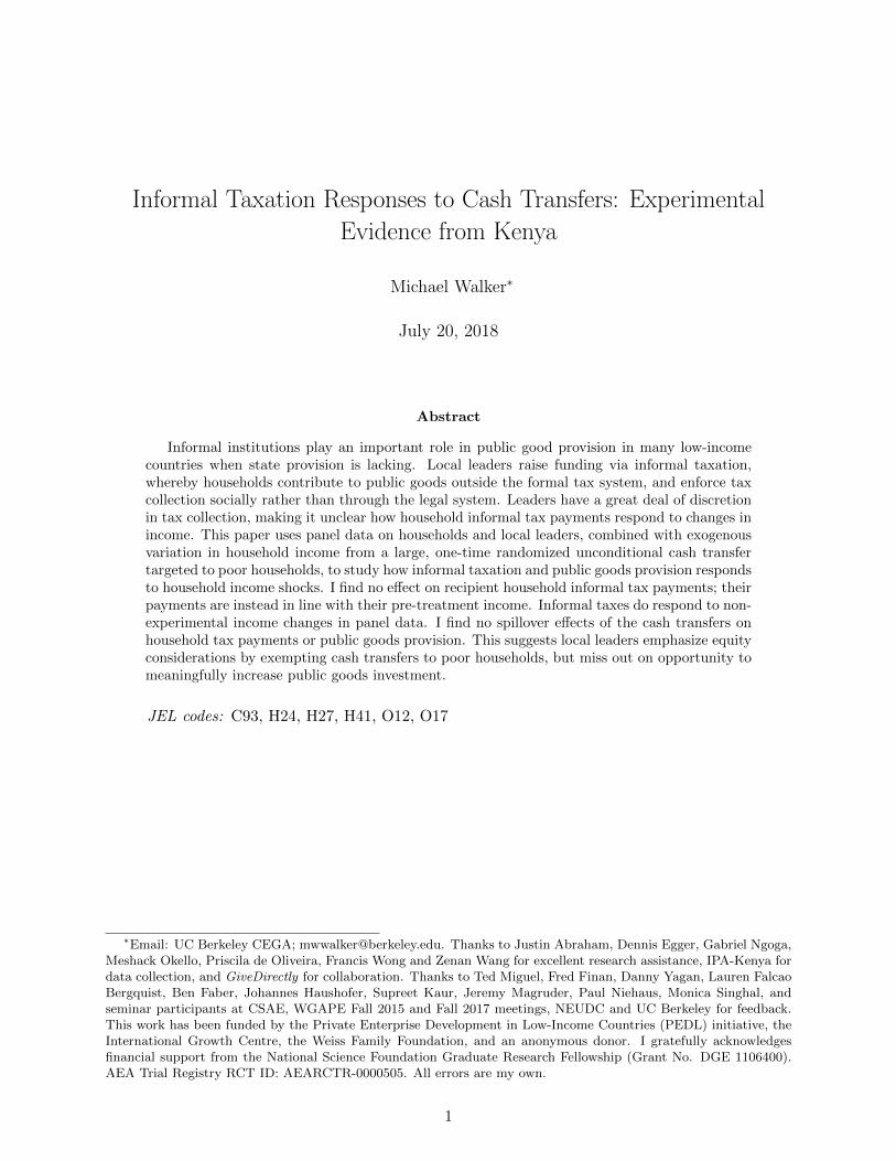
Informal Taxation Responses to Cash Transfers: Experimental

Evidence from Kenya

Michael Walker∗

July 20, 2018

Abstract

Informal institutions play an important role in public good provision in many low-incomecountries when state provision is lacking. Local leaders raise funding via informal taxation,whereby households contribute to public goods outside the formal tax system, and enforce taxcollection socially rather than through the legal system. Leaders have a great deal of discretionin tax collection, making it unclear how household informal tax payments respond to changes inincome. This paper uses panel data on households and local leaders, combined with exogenousvariation in household income from a large, one-time randomized unconditional cash transfertargeted to poor households, to study how informal taxation and public goods provision respondsto household income shocks. I find no effect on recipient household informal tax payments; theirpayments are instead in line with their pre-treatment income. Informal taxes do respond to non-experimental income changes in panel data. I find no spillover effects of the cash transfers onhousehold tax payments or public goods provision. This suggests local leaders emphasize equityconsiderations by exempting cash transfers to poor households, but miss out on opportunity tomeaningfully increase public goods investment.

JEL codes: C93, H24, H27, H41, O12, O17

∗Email: UC Berkeley CEGA; mwwalker@berkeley.edu. Thanks to Justin Abraham, Dennis Egger, Gabriel Ngoga,Meshack Okello, Priscila de Oliveira, Francis Wong and Zenan Wang for excellent research assistance, IPA-Kenya fordata collection, and GiveDirectly for collaboration. Thanks to Ted Miguel, Fred Finan, Danny Yagan, Lauren FalcaoBergquist, Ben Faber, Johannes Haushofer, Supreet Kaur, Jeremy Magruder, Paul Niehaus, Monica Singhal, andseminar participants at CSAE, WGAPE Fall 2015 and Fall 2017 meetings, NEUDC and UC Berkeley for feedback.This work has been funded by the Private Enterprise Development in Low-Income Countries (PEDL) initiative, theInternational Growth Centre, the Weiss Family Foundation, and an anonymous donor. I gratefully acknowledgesfinancial support from the National Science Foundation Graduate Research Fellowship (Grant No. DGE 1106400).AEA Trial Registry RCT ID: AEARCTR-0000505. All errors are my own.

1

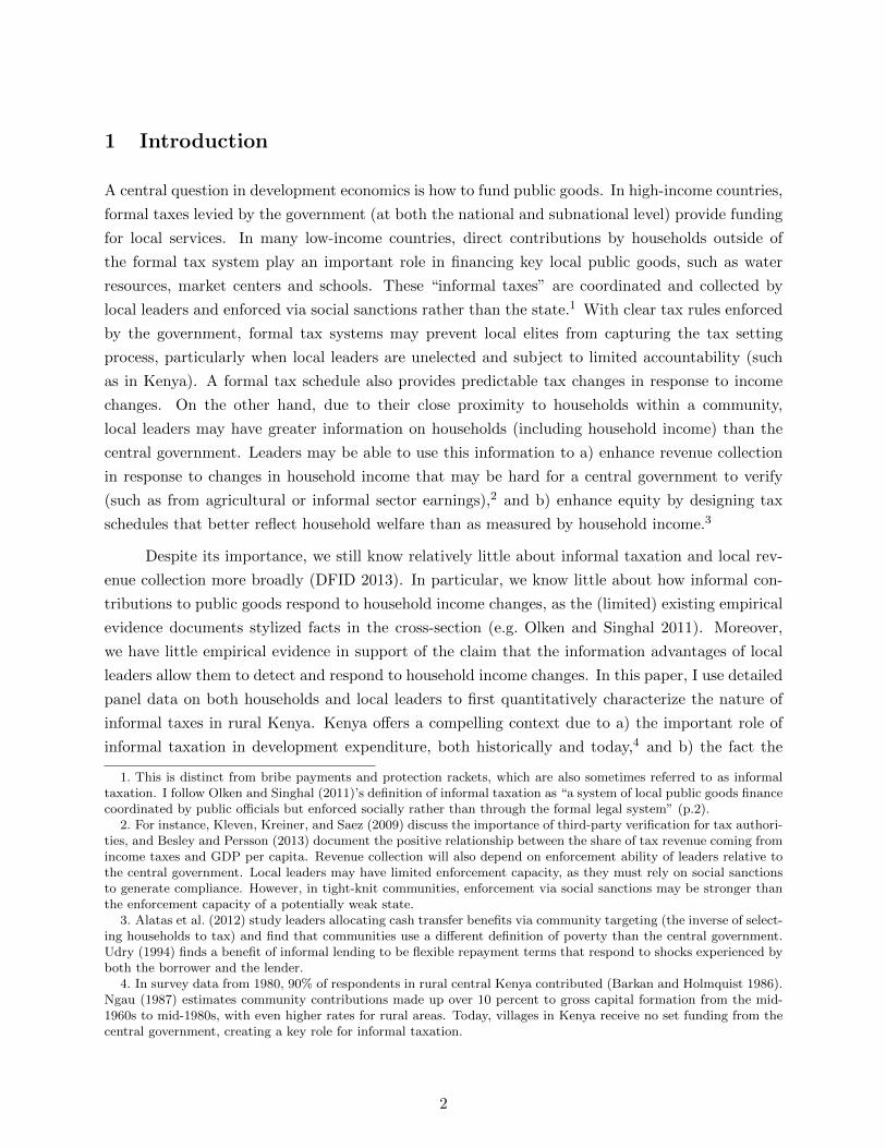
1 Introduction

A central question in development economics is how to fund public goods. In high-income countries,

formal taxes levied by the government (at both the national and subnational level) provide funding

for local services. In many low-income countries, direct contributions by households outside of

the formal tax system play an important role in financing key local public goods, such as water

resources, market centers and schools. These “informal taxes” are coordinated and collected by

local leaders and enforced via social sanctions rather than the state.1 With clear tax rules enforced

by the government, formal tax systems may prevent local elites from capturing the tax setting

process, particularly when local leaders are unelected and subject to limited accountability (such

as in Kenya). A formal tax schedule also provides predictable tax changes in response to income

changes. On the other hand, due to their close proximity to households within a community,

local leaders may have greater information on households (including household income) than the

central government. Leaders may be able to use this information to a) enhance revenue collection

in response to changes in household income that may be hard for a central government to verify

(such as from agricultural or informal sector earnings),2 and b) enhance equity by designing tax

schedules that better reflect household welfare than as measured by household income.3

Despite its importance, we still know relatively little about informal taxation and local rev-

enue collection more broadly (DFID 2013). In particular, we know little about how informal con-

tributions to public goods respond to household income changes, as the (limited) existing empirical

evidence documents stylized facts in the cross-section (e.g. Olken and Singhal 2011). Moreover,

we have little empirical evidence in support of the claim that the information advantages of local

leaders allow them to detect and respond to household income changes. In this paper, I use detailed

panel data on both households and local leaders to first quantitatively characterize the nature of

informal taxes in rural Kenya. Kenya offers a compelling context due to a) the important role of

informal taxation in development expenditure, both historically and today,4 and b) the fact the

1. This is distinct from bribe payments and protection rackets, which are also sometimes referred to as informaltaxation. I follow Olken and Singhal (2011)’s definition of informal taxation as “a system of local public goods financecoordinated by public officials but enforced socially rather than through the formal legal system” (p.2).

2. For instance, Kleven, Kreiner, and Saez (2009) discuss the importance of third-party verification for tax authori-ties, and Besley and Persson (2013) document the positive relationship between the share of tax revenue coming fromincome taxes and GDP per capita. Revenue collection will also depend on enforcement ability of leaders relative tothe central government. Local leaders may have limited enforcement capacity, as they must rely on social sanctionsto generate compliance. However, in tight-knit communities, enforcement via social sanctions may be stronger thanthe enforcement capacity of a potentially weak state.

3. Alatas et al. (2012) study leaders allocating cash transfer benefits via community targeting (the inverse of select-ing households to tax) and find that communities use a different definition of poverty than the central government.Udry (1994) finds a benefit of informal lending to be flexible repayment terms that respond to shocks experienced byboth the borrower and the lender.

4. In survey data from 1980, 90% of respondents in rural central Kenya contributed (Barkan and Holmquist 1986).Ngau (1987) estimates community contributions made up over 10 percent to gross capital formation from the mid-1960s to mid-1980s, with even higher rates for rural areas. Today, villages in Kenya receive no set funding from thecentral government, creating a key role for informal taxation.

2

redistributive implications of informal taxation are unclear.5 I then utilize an exogenous temporary

income shock from a randomized controlled trial of a large, one-time unconditional cash transfer

targeting poor households meeting a basic means-test, to empirically test how informal taxation

responds to changes in household income. To my knowledge, this is first paper to estimate the

response of informal taxes to household income changes. I estimate informal tax schedules over

the income distribution for transfer recipients and test if this schedule differs from the schedule for

control households. I test whether, in the face of this exogenous income shock, informal taxes are

assessed on households’ annual income (inclusive of the transfer). I compare estimates on informal

taxes to direct formal tax payments by households.

I also use this shock to estimate how public good provision responds to a large influx of income.

Whether public goods provision can increase via informal institutions as households experience

positive income changes is especially relevant for development policy as direct cash transfers to

households continue to scale rapidly (Faye, Niehaus, and Blattman 2015). While a large literature

finds that cash transfers help alleviate poverty for recipient households (e.g. Arnold, Conway,

and Greenslade 2011), improving public goods is a key part of the development process. Despite

the growing body of evidence on the effects of UCTs on household welfare (Arnold, Conway,

and Greenslade 2011; Bastagli et al. 2016; Evans and Popova 2014; Haushofer and Shapiro 2016),

relatively little is known about how the interaction between cash transfer programs and local public

finance institutions mediate these effects. On one hand, if a portion of unconditional cash transfers

to households is channeled into investments in public goods, this provides a mechanism for both

long-term benefits and spillover benefits to non-recipients from a one-time transfer. If public goods

are normal goods, then one would expect to see an increase in public good expenditure in response

to an increase in household income. The welfare implications for recipient households would then

depend on the relationship between their marginal benefits of private consumption versus public

goods consumption. On the other hand, if elites capture these gains and do not invest them, this

unambiguously reduces household welfare to recipient households. Similarly, if informal institutions

have low capacity or difficulty solving collective action problems, then we may not see changes, even

if the positive returns to public goods outweigh the costs.

This paper begins by documenting several cross-sectional facts on informal taxation. First,

I find that informal taxation remains widespread in Kenya: over 40 percent of households report

making informal tax payments in the last 12 months, twice the rate of direct formal tax payments.

The mean household paid 2.5 percent of its household income towards informal taxes. Second, while

informal tax participation and payments are increasing in income, higher income households pay

5. Barkan and Holmquist (1986) argue that community fundraisers may provide a progressive form of local taxationsince “rich” peasants pay more, especially than the landless. However, they do not have data on household incomesto fully quantify the degree of progressivity over the income distribution. In a similar vein with contemporary data,Zhang (2017) finds expected community fundraiser contributions to be dramatically higher for businessmen andpoliticians relative to villagers in a nearby area of western Kenya. The mean expected contribution for a businessmanwas 4 times higher than for a villager, while politicians were expected to contribute over 70 times more than avillager. In contrast, Olken and Singhal (2011) find informal taxation is regressive in 5 countries for which they havecross-sectional payment data (the Philippines, Albania, Ethiopia, Indonesia and Vietnam).

3

less as a share of income, making informal taxation in Kenya regressive. Third, informal taxation

is more regressive than formal taxation. These findings are broadly consistent with stylized facts

by Olken and Singhal (2011), though as previously noted their data does not include Kenya. The

regressive nature of informal taxation is in contrast with the hypothesis of Barkan and Holmquist

(1986). Informal taxation also provides an important source of locally-controlled funding. Villages

receive no set funding from the central government, and informal taxation plays an important

role for public good improvements, repairs and maintenance. This is especially true for water

resources, as informal taxation accounts for almost three times as much expenditure as other

external (government or non-governmental) funding.

Next, I utilize the panel nature of my data to offer new insights into the nature of informal

taxation.6 I find that the amount paid in informal taxes responds to changes in household income:

for households in control villages (i.e. those that did not a receive a transfer), a shift in income

deciles between baseline and endline is associated with a statistically significant change in informal

tax payments. Changes in household income deciles are associated with larger changes than changes

in household wealth deciles. This suggests that leaders are aware of household income changes, and

are able (and willing) to change tax amounts for households in response to changing economic

circumstances.

I then examine how informal taxes respond to a one-time exogenous income shock in the

form of an unconditional cash transfer (UCT) administered by a non-governmental organization

(NGO).7 Villages are randomly assigned to treatment or control status, and all households meet-

ing a basic means-test within treatment villages receive the UCT. Local leaders are aware of the

transfers: the NGO informed all local leaders in advance of operating within their village, and the

means-test is based on publicly observable characteristics (household roof materials).8 Both the

magnitude of the transfers and the scale of the program is large: at around US$1,000 (nominal)

per household, this corresponds to about 75% of annual expenditure for recipient households. The

UCT income dramatically shifts recipient households up the income distribution: applying the

UCT to households’ baseline (pre-treatment) income shifts all recipient households above the 90th

percentile of the baseline income distribution.9 The intervention involves almost US$11 million in

transfers and 653 villages in one Kenyan county; this is estimated to be an increase of 14 percent

of GDP across treatment villages.

The lack of a fixed informal tax schedule makes the expected informal tax response to the

exogenous income shock an empirical question; a priori, the direction of the effect is ambiguous. On

one hand, as the UCT transfer is windfall income for households, one might expect high informal

taxes for recipient households, as these would be non-distortionary. The nature of the income shock

6. The following findings are all based on panel data for control households and/or non-recipient households. SeeSection 3 for more details on the data collection.

7. Transfers are distributed by the NGO GiveDirectly (GD).8. Anecdotally, the transfers are common knowledge for all households in the study area.9. This may overstate the shift, as non-transfer income is measured with error. Nonetheless, the magnitude of the

transfer is quite large in the local context.

4

also reduces information and coordination problems for local leaders.10 The transfers are made to

poor households within the village. Poor households could be overtaxed due to their lower social

standing. On the other hand, they may be taxed less due to equity considerations.11 With no set

tax brackets, the UCT income may or may not move households into a new tax bracket in the eyes

of local leaders.

I find no significant effect on the amount of informal taxes paid by recipient households,

nor on their tax rate as a share of earned income. I also find no increase in the likelihood of

recipient households paying informal taxes (the extensive margin), nor a significant increase for

recipient households that report paying any informal taxes (the intensive margin). The observed

point estimate for the mean effect for eligible households in treatment versus control villages of

KES 14 is 0.01 percent of the total transfer value. This is also statistically significantly less than

the predicted change in informal taxes from panel estimates for control households: if the transfer

income was taxed at the same rate, we would expect to see an increase of KES 165 due to the shift

of recipient households up the income distribution, well above the upper bound of the 95 percent

confidence interval for the effect on informal taxes for eligible households of KES 53. This strongly

suggests that the transfer income is treated differently than earned income by local leaders.

I do find that recipient households pay more in formal taxes associated with self-employment.12

Recipient households in treatment villages are 2.4 percentage points (on a base of 15 percent) more

likely to pay any county taxes than eligible households in control villages; this increase is driven

by market fees that vendors pay to the county to sell in market centers. Overall, the magnitude of

the effects on both formal and informal taxes are small: point estimates suggest a total tax (formal

and informal) increase of less than 1 percent of the total amount of the UCT program.

The absence of an effect on informal taxes is surprising, given leaders are aware of transfers

and that control household shifts in the income distribution are associated with changes in infor-

mal tax payments. I estimate informal tax schedules across the pre-treatment and post-treatment

income distribution and find that leaders are taxing recipient households similarly to control house-

holds with the same baseline income, rather than household income inclusive of the transfer amount.

This is true across the income distribution: even recipient households with relatively higher pre-

10. GD informed local leaders prior to the start of their operations within a village, and while the targeting criteriaof grass-thatched roofs was not disclosed in advance, this is publicly observable for households within the village andwas easy for villagers to deduce which households received transfers.In addition, while transfers were distributed overa set of 3 payments, over 90 percent of recipient households received their payments within 3 months of the firsthousehold within the village receiving a transfer.

11. Here, I focus on household contributions to public goods. A separate issue is the degree to which households are“taxed” by family and friends (Jakiela and Ozier 2016; Squires 2017). I do find some evidence of “kinship taxation”(Jakiela and Ozier 2016, Squires 2017), as cash transfer treatment households send about 25 percent more in inter-household transfers compared to eligible households in control villages, predominately to other family members. Themagnitude of this increase is still less than 1 percent of the cash transfer value.

12. Non-recipient households in treatment villages also pay more in national income taxes (significant at a 10 percentlevel), driven by an increase in taxes paid on the intensive margin. However, only 3 percent of households reportpaying any income taxes and this may be due to an imbalance in the number of employed non-recipient householdsacross treatment and control villages. I find it unlikely that this effect is driven by the cash transfer program.

5

treatment incomes pay no more than control households with a similar pre-treatment income. This

is consistent with leaders exempting the transfer income from informal taxes.

The fact that these are one-time transfers and are targeted at poorer households, who may

otherwise have more limited earnings potential, suggests an equity consideration on the part of

the leaders. I provide some suggestive evidence that changes in permanent income are associated

with larger changes in informal taxes than changes in temporary income. Leaders thus appear to

exercise discretion and tax households more similarly to their pre-treatment rates. This highlights

an under-appreciated equity benefit of informal taxation relative to formal taxation. In settings

where income can be highly volatile, this suggests an additional appeal of informal taxation for

households.

Perhaps unsurprisingly given the lack of an effect on informal taxes, I find no increase in the

number of public goods projects, expenditures or reported quality in treatment villages.13 In the

absence of high-return projects, one would not expect to see an increase in public good spending.

However, like many rural areas in low-income countries, there is a general under-provision of public

goods. My data from local leaders suggests substantial scope for inexpensive projects with high

potential benefits.14 For example, 45 percent of households report their primary water source to

be unprotected. Protected springs, which can be constructed for US$600, confer substantial health

benefits to users (Kremer et al. 2011). Taken together with the informal tax results, this highlights

a tradeoff for local leaders: by exempting the transfer income, leaders forgo a sizable potential

revenue gain that could go towards public goods. If recipient households were taxed at the average

informal tax rate, the average village would raise US$545, similar in magnitude to the cost of

protecting a spring. Looking instead at marginal tax amounts as households move up the income

distribution, the counterfactual tax amounts for recipient households based on the schedule for

control households suggest leaders could increase expenditure on water points by over 30 percent.

As villages are unlikely to experience an influx of income of similar magnitude (about US$30,000

was sent to households in a treatment village with the mean number of eligible households), this is

a missed opportunity for improving public goods.

This paper provides valuable new insights into the informal tax literature. These findings

are most closely related to Olken and Singhal (2011), which documents similar findings on the

widespread nature of informal taxes and its regressive nature in cross-sectional microdata for 10

countries. They model informal taxation as a tradeoff between information and enforcement, and

find that the stylized facts they document in the cross-section are consistent with a model in which

informal taxes are optimal, given enforcement constraints. I build on their paper by providing panel

evidence on how informal taxes respond to both non-experimental and experimental household

13. Public goods covered by local leader surveys include water points, roads, bridges, health clinics, market centers,public toilets, cattle dips, library/resource centers, meeting halls, and other facilities leaders report that benefit thecommunity. While household survey data covers public goods contributions to schools, school projects as reportedby school head teachers will be the subject of future work.

14. For instance, the median water project in my data cost US$80.

6

income changes. It also provides support for the idea that leaders are knowledgeable of household

income changes and can respond accordingly, although they sometimes choose not to do so.

These findings shed additional light on the costs and benefits of informal institutions. For

instance, Udry (1994) documents the benefits of informal lending, and shows that the flexible

nature of loan contracts in rural Nigeria provide an additional measure of insurance for household

shocks. Jakiela and Ozier (2016) and Squires (2017) highlight a potential cost: strong egalitarian

norms about sharing windfall income lead to an efficiency cost as households seek to hide income.

I document a tradeoff between equity concerns for poor households and a missed opportunity

to make public goods investments. These findings also relate to the behavior of local leaders, a

common institution in many developing countries, including those in sub-Saharan Africa (Baldwin

2016; Acemoglu, Reed, and Robinson 2014). The fairness and equity considerations that leaders

take into account when setting informal tax amounts may be similar to those used by leaders to

select households to benefit from government programs, such as in India or Indonesia (Munshi

and Rosenzweig 2015; Alatas et al. 2012). Leaders’ role as informal tax collectors also ties into

findings by Khan, Khwaja, and Olken (2016): in response to additional incentives for tax collection,

collectors focus on a small number of high-value targets, rather than seeking to raise smaller amounts

of revenue from a larger number of people.

Lastly, these results have important policy implications for UCT programs, especially as they

scale rapidly both worldwide and in sub-Saharan Africa (Faye, Niehaus, and Blattman 2015). This

paper provides causal estimates on the response of informal taxation and public goods to uncondi-

tional cash transfer programs. My findings suggest that recipient households are not overtaxed by

elites, but that expectations for spillover or long-term benefits via public goods should be tempered

as there is no evidence for increased investment in public goods. Importantly, I do not find negative

effects on public good provision. The UCTs do reach their intended targets and benefit recipient

households, but this one-time positive income shock does not translate into increased public goods

investment, turning off a potential channel for spillover benefits to non-recipient households.

The rest of this paper is organized as follows. Section 2 provides background information

on the informal and formal tax system in rural Kenya. Section 3 describes the data, and Section

4 quantifies informal taxation in Kenya, making use of non-treatment data. Section 5 provides

details on the UCT intervention, experimental design, and empirical specifications used to estimate

the effects of UCTs on informal taxes and public goods. Section 6 presents the main results on the

effects of UCTs on informal taxes, with Section 6.2 outlining how recipient informal tax amounts

are in line with baseline income. Section 7 presents results on public goods. Section 8 discusses the

results, including potential alternative mechanisms, and Section 9 concludes.

7

2 Background

This section describes the study setting, including how informal taxation works in rural Kenya. It

introduces the key local leaders and types of tax collections that matter for understanding the data

collection outlined in Section 3, and sets the stage for the quantitative analysis of informal taxation

outlined in Section 4.

2.1 Study Setting

This study takes place in Siaya County, Kenya, a populous rural area in the western Kenya region

of Nyanza bordering Lake Victoria.15 Siaya County, like the rest of Nyanza, is predominantly Luo,

the second-largest ethnic group in Kenya. In data from the 2009 Kenyan census, Siaya is at or

below the median on available development indicators (see Table B.4). The study sample consists

of 653 villages containing approximately 65,000 households spread over 3 contiguous constituencies

within Siaya County. Villages are the lowest administrative unit in Kenya. Study villages contain a

mean of 100 households, and range from a minimum of 19 households to a maximum of 245 (Table

B.3, Panel A).

2.2 Informal taxation in rural Kenya

Revenue collection by local leaders in Kenya extends back to the colonial period. The British

introduced a hut tax (collected per household) in 1902 and a poll tax (on each individual) in 1910.

District officers used local leaders as hut counters and tax collectors, and leaders had discretion to

exempt households that were unable to pay (Gardner 2010). In addition to informal taxes collected

directly from households, Kenya also has a particular institution of informal taxation known as

harambees. These public fundraising ceremonies have played a central role in development policy

since independence (Barkan and Holmquist 1986; Ngau 1987). Revenue collection (including via

harambees) is typically done to support a particular project or cause.

In rural Kenya (as in many other areas), local leaders, rather than the government or public

utilities, oversee key public goods. For example, rather than municipal water services provided by

a public utility, many households rely on public springs and wells, along with natural lakes and

streams, for water. These public goods have important implications for the health and livelihoods

of households within their jurisdiction. However, in the Kenyan context, local leaders do not

receive a dedicated budget from the government, so they must either find external funding or raise

money from households within their jurisdiction via informal taxation. To raise external funding,

15. This paper is one component of a broader investigation into the general equilibrium effects of cash transfers (the“GE” project) (Haushofer et al. 2014). The focus on tax and public goods effects was included as part of the studyregistration.

8

leaders can solicit funding from politician-led development funds or NGOs.16 Local leaders collect

informal taxes from households in order to maintain, repair and improve public goods in their

jurisdiction. Funding is typically raised for a specific project or purpose. In this way, local leaders

serve as “development brokers” (Baldwin 2016). Local leaders thus consider the costs and benefits

of a project to households in their jurisdiction, their own effort costs and their own payoff (from

households) of completing a project. The urgency and amount of money to be collected will depend

on situation on the ground.

There are several types of local leaders relevant to this study. Villages are overseen by a

village elder (VE), an unsalaried position appointed by the assistant chief (AC).17 ACs administer

sublocations, the administrative unit directly above the village level; sublocations in the study

area contain an average of 10 villages. ACs are the lowest-level administrator that is salaried

by the national government and are appointed by chiefs (who administer locations). Due to the

governmental salary, AC appointment is competitive. There are no set term limits for either VEs

or ACs, and limited upward advancement within either position. Assistant chiefs and village elders

are required to be residents of the village / sublocation that they administer; typically these are

also the “home areas” where the leaders grew up and have longstanding familial ties.

In addition to assistant chiefs and village elders, primary school headmasters can also be

involved in raising and collecting funds for school projects. Primary education is de jure free in

Kenya, yet all schools still charge a number of fees to attend. In addition to school fees, school

headmasters may also have collections for specific development projects. While parents of children

in school are typically expected to contribute to these school development projects, members of the

community without children in school may also be expected to contribute, particularly via events

such as harambees. Headmasters may also recruit village elders and assistant chiefs for help in

enforcing payment (Miguel and Gugerty 2005).

Informal taxes can take the form of cash, labor or in-kind material contributions.18 Tax

collection can take a variety of forms. Leaders can hold a village meeting to assign contributions,

or, for larger projects, can hold a harambee, a community fundraiser. All harambee attendees are

expected to contribute, and invited “guests of honor” are expected to make especially large contri-

butions (Zhang 2017). Contributions are made in public, so they are highly visible. Contributions

can also be made via a pledge cards, whereby numerous households list the amount they are pledg-

ing to contribute on a single piece of paper. Households would then remit the money at a later

date. Contribution amounts are again publicly observable to anyone that sees the pledge card, and

may also serve as an improved enforcement mechanism for leaders, as they can reference the card.

The public nature of the collections, and the specific purpose for which funds are typically raised,

16. Both Members of Parliament (national-level politicians) and Members of the County Assembly (county-levelpoliticians) have development funds for use on projects in their constituencies.

17. While the position is unsalaried, it does carry the potential for remuneration: for example, VEs frequentlyreceive an “appreciation” payment for their time when resolving disputes or serving as guides to NGO field workers.

18. Materials may be directly relevant to a project, for instance contributing sand or bricks to a construction project,or may take the form of in-kind agricultural payments.

9

may also help diminish graft on the part of leaders. Lastly, leaders can also go door-to-door for

collections. Leaders may exercise discretion in the households that they choose to visit.

The primary method of payment enforcement is via social sanctions. Leaders may make public

announcements of non-payment, work with clergy to encourage contribution reminders in sermons,

and home visits (Miguel and Gugerty 2005). In the case of contributions to public goods at schools,

children can be sent home for non-payment. Non-payment could also result in exclusion from

informal insurance arrangements, as leaders take past contributions into account when deciding

whether to take up collections for households for events such as funerals or weddings.19

2.3 Formal taxes in rural Kenya

While over 40 percent of households report paying informal taxes in the study area, only 20 percent

of households report paying any direct formal taxes. Kenya has two levels of government: the na-

tional government and the county governments. Each of these collect different types of taxes. The

national government is responsible for income taxes. In practice, this is only paid by employees in

the formal sector, where it is paid on a pay-as-you-earn basis and is taken directly out of employees’

paychecks. The fact this is only paid by formal sector workers is due in part to exemptions: subsis-

tence agriculture and pastoral activities are not subject to taxation. As 97 percent of households in

our baseline data engaged in these activities, this is an important exemption for rural households.

Given that much of this own production is consumed by households, income from these activities

would be hard for the government to verify, though it would be easier for local leaders to assess.

Second, transfer income (either from remittances or NGOs) is not subject to taxation, though any

additional revenues these transfers generate is subject to tax.20

The main county taxes are associated with self-employment: enterprise license fees and market

fees. All self-employed businesses are supposed to be licensed by the county government, even those

that operate in the informal sector. There are specific fees for small vendors and traders. Market

fees are paid by vendors when they sell from formal markets. At baseline, 90 percent of households

making formal tax payments only make payments to the county government.

19. Note that my results focus on collections for public goods. I find that recipient households increase theirmembership in community groups; while this is not the same as engaging in risk-sharing networks, it is suggestivethat they are not opting out and that this channel is not driving my results.

20. Tax systems in developed countries vary in their treatment of income analogous to the UCT transfer income. Inthe US tax system, lottery, gambling winnings and prizes are taxable and count towards a household’s annual income.However, gifts do not count as income for recipient households, and IRS regulations are vague on whether transferssuch as these would be considered income. In the case of gifts and charitable assistance for disaster relief, the taxcode is clearer. However, there are numerous conflicting reports about how the IRS treats crowdfunding income.Inthe Netherlands, winnings from the Dutch postcode lottery (analogous in that neighborhoods of households thatchoose to buy lottery tickets receive an income transfer) are taxed and count as income. In the UK, winnings fromthe postcode lottery are not taxed.

10

3 Data

There are no official records of informal tax collection from households at the village level in

rural Kenya. In addition, as villages and sublocations receive no set funding from the national or

county government, there are no administrative records of public goods projects or spending at

the village level. A particular strength of this project is the use of original data collected from

both households and local leaders explicitly designed to look at informal taxation and local public

finance. Household surveys cover a representative sample of households, allowing me to look at the

full income distribution in rural Kenya. I am able to make comparisons with the cross-sectional

stylized facts established by Olken and Singhal (2011), and to provide new evidence on the manner

in which informal taxes respond to income changes using panel data. Local leader surveys included

collecting a listing of all public goods within the village, and, for each public good, a listing of all

development projects (improvements, repairs and maintenance) since 2010. This section describes

the household and local leader data.21

3.1 Household Data

Data on households comes from two rounds of in-person surveys, a baseline survey round conducted

in advance of the cash transfer intervention and an endline survey round conducted an average of

19 months after the baseline survey (range of 9 to 31 months; see Figure 5).22 Research team

enumerators first conducted a census of all households within the village. The census collected

information on the household’s name, contact information, housing materials, and GPS coordi-

nates. Data on household housing materials was used to calculate eligibility for the UCT (whether

households have a thatched roof) and as a proxy for village wealth. This census data serves as

the sampling frame for household surveys and as the basis for village population calculations when

constructing village-level per-capita outcomes.

Households were randomly sampled to be surveyed from village census data. Baseline surveys

targeted 12 households per village, 8 thatched-roof households and 4 non-thatched roof households.

For married/coupled households, either the male or female was randomly selected to be the “target”

respondent; if we could not reach the target, but the spouse/partner was available, we surveyed the

spouse/partner. If a sampled household was not available to be surveyed on the day the field team

visited the village for baseline surveys, the household was replaced with another randomly-selected

household. Household baseline activities began in August 2014 and concluded in August 2015, with

a total of 7,845 households surveyed.

A second (endline) round of household surveys were conducted between May 2016 and May

21. In section 5.2, I return to describe how data collection fit in with the experimental intervention.22. Due to the large size of the intervention, villages received cash transfers on a rolling basis. Within each

treatment village, baseline surveys were conducted prior to the distribution of any cash transfers.

11

2017, with the majority of the surveys coming between June 2016 and January 2017.23 Endline

surveys targeted both households that were baselined and households that were intended to be

surveyed but unavailable at baseline. This led to a total target of 9,150 households, of which 90.1

percent were successfully surveyed. Column 4 of Table B.1 shows that tracking rates are balanced

across treatment and control villages, both overall and by eligibility status. Of households surveyed

at endline, 87 percent of these were also surveyed at baseline, which is also balanced across treatment

and control villages. Of households that were missed at baseline, 78 percent were surveyed at

endline.

This provides three different samples for household-level analyses: a baseline sample of 7,845

households surveyed at baseline, an endline sample of 8,240 households surveyed at endline, and

a panel sample of 7,224 households surveyed at both baseline and endline. When establishing

stylized facts on informal taxes, I make use of either the baseline or panel samples; when I use

the panel sample, I restrict attention primarily to households in control villages (a total of 3,593

households), though in order to increase statistical precision I also examine some outcomes for

all non-recipients (households in control villages plus households not eligible for GD assistance),

a total of 4,831 households. When turning to the effects of an exogenous income shock via an

UCT on household taxes, I focus on the endline sample, though I make use of baseline values

of the dependent variable when available to improve statistical precision (McKenzie 2012). I use

household census data in order to construct survey weights that account for the share of eligible

and ineligible households per village surveyed at baseline, endline and in both rounds in order to

properly represent the share of eligible versus ineligible households in the study population.

Both rounds of the household survey collected information on respondent demographics,

economic activity (agriculture, self-employment and employment), asset ownership and formal and

informal taxes, among other variables. Informal taxes include cash payments, labor contributions

and the value of in-kind materials to public goods. Surveys also capture charitable and social

assistance (such as burial or wedding contributions), which I consider separate from informal taxes.

In addition, endline surveys include information on household expenditure, transfers to and from

other households, and crop-by-crop agricultural production.

Table 1 provides summary statistics at baseline by analysis sample and by transfer eligibility

status. The mean household contains 4.3 members at baseline, 2 adults and 2.3 children. 75 percent

of respondents are female, with 64 percent of respondents married / cohabitating and 34 percent

widowed or widowers. The mean age of respondents is 48, though households eligible for a UCT are

significantly younger on average than ineligible households.24 Almost all (97 percent) of households

are engaged in agricultural, while a quarter of respondents are engaged in self-employment and

another quarter are engaged in wage work. Eligible households are more likely to engage in wage

23. In addition to tracking households in our Siaya study area, we also surveyed households that migrated outsideof our study area, surveying households in Nairobi, Kisumu (the largest city in western Kenya) and other towns inwestern Kenya.

24. This is sensible if one expects households to accumulate wealth over the course of their lifecycle.

12

work than ineligible households.

3.2 Local Leader Data

Local leader surveys targeted village elders (VEs), who oversee villages, and assistant chiefs (ACs),

who administer sublocations, the administrative unit directly above the village. Sublocations in

the study area contain an average of ten villages. As previously noted, there are no formal records

of public goods projects and spending at the village or sublocation level in Kenya, though village

elders and assistant chiefs may keep their own records. The primary goal of the local leader surveys

is to construct a panel dataset on local public goods, development projects, and fundraising at the

sublocation and village level from 2010 to 2016. Village elders for all 653 villages in the GE study

sample and assistant chiefs for all 84 sublocations that contain at least one GE project village were

targeted for surveys.25

I conducted two rounds of local leader surveys. Surveys elicited a listing of the public goods

within each village or sublocation, then, for each public good, a listing of any projects, including

new constructions, repairs and improvements, and cash, in-kind, land and labor contributions to

these projects from both households and external sources. Surveys also collect information on

regular upkeep activities (such as clearing brush) occurring in the previous 12 months for both

survey rounds. In round 1, which ran from July to December 2015, the goal was to construct a

retrospective panel of public goods and development projects going back to 2010. The second round,

which primarily ran from July to December 2016, covers development projects going back to August

2014, the month before any treatment began. If, in round 2, survey enumerators encountered

projects that should have been collected as part of round 1, but were not, skip patterns in the

survey prompted enumerators to collect retrospective information back to 2010 for these projects.

Surveys concentrated on the most relevant for types of public goods for local leader, based on the

geographic scope of the benefits for public goods and leader knowledge of projects determined via

extensive survey piloting. For village elders, questions about public goods focused on water points

and feeder roads, while assistant chief surveys focused on health clinics and market centers, all

of which serve multiple villages.26 Both village elders and assistant chiefs are asked about other

public facilities that are more rare, such as public toilets, playing fields and meeting halls. Taken

together, this provides a dataset of over 3,000 public goods and over 4,000 projects from 2010 to

2016.

25. GD defined villages based on 2009 Kenya Population Census enumeration areas. In some cases there canbe more than one village elder in a single GD village if villages (as they exist outside of for purposes of censusenumeration) were combined into a single enumeration area. In cases where there is more than one VE within avillage, enumerators were instructed to interview all of the village elders for that village. I then aggregate outcomesto the GE village (in other words, the census enumeration area), as this was the lowest level at which treatment wasrandomized.

26. Note that this excludes primary schools. A separate survey was fielded for school headmasters, which will bethe subject of future work.

13

Both survey rounds had high tracking rates for VEs and ACs (Table B.2).27 Columns 4

and 8 of Table B.2 report t-tests for differences in the mean tracking rate by treatment status;

for villages, this tests for differences in survey rates between treatment and control villages, while

for sublocations, this tests for differences between high and low saturation sublocations. A greater

share of control villages were surveyed as part of round 2 (statistically significant at the 10% level),

though we surveyed 97% of treatment villages and 99% of control villages.

4 Quantifying informal taxation and public goods in Kenya

I now turn to quantitatively characterizing the nature of informal taxation in rural Kenya using

my unique panel data on households and public goods. I map the full informal tax schedule across

the income distribution for households. From this, a number of key facts emerge. First, informal

taxation is widespread: 43 percent of households report paying informal taxes, over twice the

rate of households paying formal taxes. Second, informal tax amounts are increasing in household

income and wealth, but declining as a share of household wealth. This implies informal taxes are

redistributive but regressive. Third, I show that informal taxes are more regressive than formal

taxes. These first three facts echo findings from Olken and Singhal (2011) in their cross-sectional

data.

Fourth, using panel data, I show that the amount paid in informal taxes responds to changes

in household income. A shift up an income decile is associated with a statistically significant change

in the amount paid in informal taxes. The magnitude of a shift up an income decile is about twice

as large as a shift up a wealth decile. As in the cross-section, these shifts result in larger increases

in formal taxes relative to informal taxes, again implying that informal taxes are more regressive

than formal taxes. This also suggests that local leaders are able identify and more heavily tax

households that see an increase in their household income.

Fifth, while informal taxation may make up only 2-4 percent of household income, it provides

an important source of locally-controlled funding for local public goods. I also find that there is

potential for low-cost investments in water resources that could lead to high returns by reducing

water-borne illnesses, especially for children.

I measure informal taxes as the sum of household cash, labor and the value of in-kind contri-

bution to public goods (via harambees or other means), school project contributions (distinct from

school fees for attendance), and village elder taxes (this includes items such as community celebra-

tions and community policing). I value labor contributions at the median agricultural (unskilled)

wage as reported by village elders in control villages.28 In terms of formal taxes, I focus on direct

27. All ACs were surveyed in both rounds, though 11 (13 percent) were unable to be reached during the mainperiod of local leader surveying (July to December 2016) and were instead surveyed in the subsequent seven months.Tracking rates remain balanced, and results are quantitatively and qualitatively similar, regardless of whether theselater surveys are included. My main tables include these surveys.

28. Village elders were asked about the daily wage for hiring a casual worker for a variety of agricultural activities

14

formal taxes paid to the national and county government, and do not include indirect taxes.29

In what follows, I use household income, rather than expenditure (as is common in much of

the development literature), despite the potential for measurement error in household income. I

do this for several reasons. Income has a more direct analogue to the public finance literature. I

also can construct measures of household income for both baseline and endline, while I only see

household expenditure at endline. In addition, I am frequently making comparisons across income

deciles, rather than using the exact value reported by households. To the extent that this decile

ranking remains unchanged by measurement error, my main results are unaffected.30 I define

household income as the sum of household agricultural profits, self-employment profits, and wage

earnings.31 Household wealth is measured as the sum of household durable assets, livestock, home

and land value.32

4.1 Informal taxes are widespread, increasing in income, but regressive

I begin by documenting cross-sectional patterns using baseline household survey data. Informal

taxation in rural Kenya is widespread: over 40 percent of households report paying any informal

taxes in the baseline data, over twice the share of households paying formal taxes. Participation

in informal taxes is increasing in income. Panel A of Figure 1 plots the overall household income

distribution. The gray vertical lines denote income deciles, which I utilize in Panels B through D.

Panel B plots the mean share of households making any informal tax payments (in cash, in-kind or

labor) by income decile, while the bars plot the upper and lower 95 percent confidence intervals.

The share of households paying any informal taxes is rising in income; likewise, the mean amount

paid in informal taxes is also rising with income (Panel C). The relationship between income deciles

and informal tax amounts is positive over the full income distribution, but relatively flat over the

first 3 income deciles, and the fourth through sixth income deciles, suggesting that the marginal

informal tax on income in certain ranges may be relatively small. In Panel D, we see that higher

income households pay less in informal taxes as a share of their income. There is likely measurement

error and underreporting of income in this setting (like many development settings), so the income

(i.e. clearing, weeding, etc.). I take the median across all types of agricultural activities, and I assume 6 hours workedper day to convert to an hourly wage.

29. The main indirect tax is a value-added tax, but agricultural products are exempt from VAT. In enterprise datafrom the study area, less than 1 percent of enterprises report paying VAT; these are all establishments selling alcohol,which are more heavily regulated.

30. As a robustness check, I reproduce these findings focusing on wealth and/or household expenditure in theappendix.

31. Endline household surveys collected additional data on agricultural production relative to baseline. My preferredmeasure of baseline agricultural profits transforms baseline measures of agricultural sales, land use, number of workers,input costs and types of crops produced into a measure of crop production based on the endline relationship betweenthese variables and reported endline crop production for control households. I then subtract off baseline agriculturalcosts to get a measure of agricultural profits.

32. Household home value is measured by asking respondents for the cost of building a home like theirs, includingall labor and material costs. Land values are calculated by multiplying amount of land households report earning bythe households’ reported cost of an acre of land in the village.

15

shares may be overestimates. However, the fact that informal taxes are regressive holds when using

household wealth instead of income (Appendix Figure A.1).33 Even at 1 to 2 percent of household

income (half of the rate I estimate for households in the bottom half of the income distribution),

informal taxes would not be trivial for poor households, and these amounts fall within the range

found by Olken and Singhal (2011) as a share of expenditure across 10 countries.

The schedules shown in Figure 1 pool data across all villages. To quantify the degree of

regressivity within communities, I estimate OLS regressions with village fixed effects for partici-

pation and the amount paid in informal and formal taxes as a function of the natural logarithm

of household income, household expenditure and per-capita household expenditure. Here, I use

endline data from control villages, as this allows me to compare the income results with household

expenditure. These results are presented in Table 2. Panel A shows results of the linear probability

model:

Pr(AnyTaxPaymenthvs) = αv + γ lnXhvs + εhvs, (1)

where Xhvs is either household income, consumption or per-capita consumption and αv represents

village fixed effects. Standard errors are clustered at the village level, and households are weighted

to reflect their overall share in the population.

The first three columns of Table 2, Panel A present results using an indicator for any informal

tax payment, while the last 3 columns present results using an indicator for any formal tax pay-

ment. Conditional on village fixed effects, participation in informal taxes is increasing in household

income and household expenditure, though participation appears flat with respect to per-capita

expenditure. Participation in formal taxes is increasing in all three variables, and increasing more

rapidly than for informal taxes.

In Panel B, I turn to the amount paid, substituting in the total tax amount paid for the

indicator for any tax payment in equation (1). Point estimates show the increase in informal

or formal taxes paid in response to a 1 percent increase in income or consumption. Here again,

we see a positive gradient, as higher-income households pay more in both informal and formal

taxes. The coefficients on formal taxes are much larger than those on informal taxes, indicating

that formal taxes are more progressive than informal taxes. I calculate the implied elasticity of

informal and formal taxes with respect to household income, household consumption, and per-

capita consumption when evaluated at the mean informal or formal tax payment amount. I find

much higher elasticities for formal relative to informal taxes, again implying that formal taxes are

more progressive than informal taxes. The magnitude of the informal tax elasticities echoes the

findings from Figure 1: while informal taxes are increasing in income, they increase less than 1 to

1, so richer households pay less as a share of total income. Lastly, in Panel C, I estimate log-log

regression specifications among households that report paying positive amounts of informal and

formal taxes. Here, the coefficients themselves are the elasticities, and I find similar patterns as

33. Interestingly, informal taxes as a share of household wealth are on the low end, but within the range, of typicalUS property tax rates.

16

Panel B.34

4.2 Informal taxes respond to income changes

So far, I have shown that, in the cross-section, informal taxes are i) widespread, ii) increasing in

income but regressive, and iii) more regressive than formal taxes. I now use households in control

villages (where transfers were not distributed) to look at how informal taxes change in response to

household shifts in income and wealth deciles. I estimate the following equation for both income

and wealth on control households surveyed at both baseline and endline:

∆InformalTaxhv = α+ β∆Decilehv + εhv (2)

where ∆InformalTaxhv subtracts the amount paid in baseline informal taxes from the amount

paid in informal taxes at endline. ∆Decilehv subtracts either the baseline income or wealth decile

from the endline decile, depending on the specification. I cluster standard errors at the village level.

Table 9 presents the results. A one decile increase in a household’s income decile is associated with

a KES 33 increase in informal tax payments, statistically significant at the 5 percent level (column

1). Based on this point estimate, shifting up 5 income deciles (the average shift in income deciles for

transfer recipients) is associated with an increase of KES 165 in informal taxes, a 50 percent increase

in informal tax payments for a typical recipient household. This is the predicted magnitude of the

increase in informal taxes for recipient households under the assumption that the cash transfer

income counts towards a household’s informal tax base in the same way as earned income. I will

return to this when discussing the effects of the cash transfer on informal taxes.

I find that moving up a wealth decile is also associated with a positive, but not statistically

significant, increase in informal tax payments. The point estimate of KES 16.7 is half the magnitude

of the point estimate for a shift in income deciles (column 2), and this pattern holds when including

both changes in income deciles and changes in wealth deciles together (column 3). 35

I also document that shifts in income and wealth deciles are associated with statistically

significant changes in formal taxes (columns 4 through 6). As in the cross-section, the magnitude

of the effects for changes in formal taxes are larger than for changes in informal taxes, roughly by

a factor of 5. When including both changes in income and wealth deciles, the effect on income is

larger by a factor of 3 and statistically significant, in contrast to the effect on wealth (column 6).

This again implies that informal taxes are more regressive than formal taxes.

34. As a robustness check, and for comparison to Olken and Singhal (2011), I also estimate these results using aconditional logit fixed-effects model instead of the linear probability model in Panel A, and a fixed-effects Poissonquasi-maximum likelihood model for Panels B and C. The use of the Poisson model allows on to get an elasticityfrom a single estimating equation in the presence of many zero values for tax payment amounts. Both the overallpatterns and magnitudes of the elasticities are quantitatively similar (results not shown).

35. While changes in the income and wealth distribution both capture shifts in households’ relative standing to oneanother, given that values of household wealth are larger than household income, it may take a larger shock to movehouseholds from one wealth decile to the next than from one income decile to the next.

17

4.3 Informal taxes serve as important source of public goods expenditure

Given that local leaders do not have dedicated budgets, informal taxes serve as an important source

of locally-controlled revenue. This is especially true for public goods such as water points, where, in

an average year, almost 3 times as much funding comes from informal taxes compared to external

sources (Table 3). Even for roads and bridges, while external sources provide more funding on

average in a year, only 12 percent of villages receive any outside road funding, leaving local leaders

to raise funding via informal taxes for basic repair and maintenance. In addition, many of the

projects undertaken by villages are small, especially for water points, for which funding primarily

comes from local sources (Figure 2, Panel B). Table 3 also highlights the scope for additional public

goods investment in water points, as 54 percent of villages contain an unprotected spring or well.

In household survey data, 45 percent of households report that their primary water source is not a

protected spring or well. Protected springs can offer substantial health benefits: incidences of child

diarrhea drop by 25 percent (Kremer et al. 2011).

5 UCT Intervention and Experimental Design

I now turn to the UCT intervention, which provides a large, one-time, exogenous shock that can

be used to test whether local leaders tax households at their annual income.

5.1 Intervention

UCT programs are growing in popularity as a tool for poverty alleviation. Proponents of uncon-

ditional cash transfers appreciate that i) they allow recipients to spend money as they find most

effective, providing a greater range of options for recipients than in-kind aid programs; ii) they have

low administrative costs because there is no need for procurement, training, or monitoring, so a

greater proportion of funds can be provided as direct assistance (Margolies and Hoddinott 2015);

and iii) a large set of existing evidence finds positive benefits for recipient households (Arnold, Con-

way, and Greenslade 2011; Bastagli et al. 2016; Haushofer and Shapiro 2016) and that households

do not spend transfers on temptation goods (Evans and Popova 2014).

The NGO GiveDirectly (GD) provides unconditional cash transfers to poor households in

rural Kenya. For this study, GD targeted households living in homes with thatched roofs, a basic

means-test for poverty; one-third of households in our study villages are eligible for transfers based

on this criteria. GD enrolled all eligible households in treatment villages, while no households in

control villages receive transfers. Recipient households receive a series of 3 payments totaling about

US$1,00036 via the mobile money system M-Pesa.37 This transfer amount is large, and corresponds

to roughly 75 percent of annual household expenditure for recipient households. This is a one-time

36. The total transfer amount is 87,000 Kenyan Shillings (KES). The exchange rate is rounghly 100 KES = 1 USD.37. For more information on M-Pesa, see Mbiti and Weil (2015) and Jack and Suri (2011).

18

program and no additional financial assistance is provided to these households after their final large

transfer.

Two aspects of the transfer program are especially notable: first, the magnitude of the

transfer is sufficiently large to temporarily shift all cash transfer treatment households above the

90th percentile of the baseline income distribution; the median cash transfer treatment household

moves to the 97th percentile. Figure 3 displays this shift in the income distribution graphically,

with the dotted line representing the income distribution after incorporating the transfer value to

recipients.

Second, it is public knowledge to both leaders and households that GD is working in a village.

Prior to starting work in a village, GD informs local leaders they plan to operate within the village,

and hold a village meeting (baraza) with all households within the village to introduce their program

and organization. Next, GD conducts a census of all households within the village and collects

information on housing status to determine eligibility. GD then returns for two additional visits

with eligible households: in the first, household eligibility is confirmed and households are enrolled

in GD’s program; at this point households learn they will be receiving transfers. A second, final

visit (“backcheck”) by a separate GD team checks the eligibility status of all enrolled households

in advance of the distribution of transfers to ensure no gaming by households or GD staff. (A full

outline of GD’s household enrollment process is provided in Appendix B.1.)

The eligibility criteria are not provided to leaders or households at any point in the process

to prevent gaming by households. However, given that whether or not a household has a thatched

roof is publicly observable, it is not difficult to deduce, and anecdotally both leaders and households

in the study area are aware of the criteria.38

Due to the large number of villages and households involved in the study, GD worked on a

rolling basis across villages in the study area following a random order described in the next section.

GD generally began sending transfers to eligible households within a village once at least 50% of the

eligible households (as identified via the census) completed the enrollment process. Villages that

were above this threshold but in which GD was still working on completing the enrollment of other

households would see a difference in the timing of transfers to households. If households delayed

in signing up for M-Pesa, this would also introduce delays in their transfers and differences across

villages. If households reported issues arising due to the transfers (such as marital problems or

other conflicts), transfers may be delayed while these problems are worked out. GD sent payments

in batches once per month, on or around the 15th of the month. Households that did not complete

the enrollment process or register for M-Pesa in advance of the payment date one month would

thus receive transfers one month later.

The intervention was implemented as anticipated. Figure B.2 displays the cumulative percent-

age of first transfers sent to households within a village. On average, 60% of recipient households

38. Many households in control villages are also aware of GD and the program eligibility criteria as well.

19

received transfers in the first month that GD sent transfers to a village, 91% have received after 6

months and 97% have received after 12 months. Figure B.3 plots the distribution of all transfers to

households within the village, with the black line referencing two and eight months after the first

transfer, GD’s schedule.

Existing evidence finds positive benefits of GD’s program for recipient households: Haushofer

and Shapiro (2016) conducted an impact evaluation in 2012 and found recipient households expe-

rienced a 61% increase in the value of assets, a 23% increase in expenditures, as well as improved

food security and psychological well-being. Recipients of the cash transfer in this study did indeed

benefit as well: compared to eligible households in control villages, eligible households in treatment

villages saw an increase of 39 percent in non-land wealth, 12 percent in household consumption and

7 percent in earned income (calculated as agricultural profits, self-employment profits and wage

earnings) an average of 18 months after the distribution of transfers (Haushofer et al. 2017).39

Recipient households are 4 percentage points (on a base of 46 percent) likely to have a household

member in self-employment. In addition, recipient households make visible investments, partic-

ularly in housing, as they report 57 percent higher values of their housing materials compared

to control households, further suggesting that households are spending the transfers in ways that

would be identifiable to local leaders. These results reinforce the large literature on the positive

benefits of cash transfers to recipient households, and the rest of the findings on taxes and public

goods outlined below should be interpreted in light of this.

5.2 Experimental Design

GD identified target villages in the study area for expansion; in practice, these were all villages

within the region that a) were not located in peri-urban areas and b) were not part of a previous

GD campaign. This resulted in a final sample of 653 villages, spread across 84 administrative

sublocations (the unit above a village), and 3 subcounties.40 On average one-third of households

in each village meet GD’s eligibility requirement, with a range from 6 to 64 percent of households;

this distribution is balanced across treatment and control (see Appendix Table B.3, panel A and

Appendix Figure B.1). Randomization was done at two levels: first, sublocations (or in some cases,

groups of sublocations) were assigned to high or low saturation status. Then, within high saturation

groups, two-thirds of villages were assigned to treatment status, while within low saturation groups,

one-third of villages were assigned to treatment status. As noted above, within treatment villages,

all households meeting GD’s eligibility criteria receive a cash transfer. Figure 4 displays the study

design graphically.

39. By recipient households, I mean households in treatment villages classified as eligible by GE research teamsurvey enumerators during household censuses. While the GE census sought to replicate GD’s census as closely aspossible, it is possible for classification by GE enumerators to differ from GD’s classification. These estimates arethus analogous to intention-to-treat results.

40. Villages are based on census enumeration areas from the 2009 Kenyan Population Census, which served as asampling frame.

20

Given the large study size, surveys and the distribution of transfers were done on a rolling

basis. Baseline household censuses and surveys were conducted prior to the distribution of any

transfers within a village. GD had plans for the order in which they would visit the three subcoun-

ties within our study area, and aimed to complete enrollment in one subcounty prior to moving to

the next. The order in which GD visited villages was randomized by clusters of villages within each

subcounty; within each cluster, the order of villages was also randomized.41 I use the randomized

village order to define an “experimental treatment start month” for all villages in the study evenly

allocating villages over the months GD began distributing transfers to villages within each sub-

county (see Haushofer et al. 2016, for full details). This provides a start date for control villages in

addition to treatment villages and ensures that the month in which treatment villages first received

transfers is not endogenous to conditions on the ground that influenced implementation.

Figure 5 displays both the calendar timeline of household surveys and transfers and the timing

of surveys and transfers relative to the experimental start date for each village. Figure B.4 visually

displays the experimental design in our study area, including the amount distributed in transfers

as of December 2016, at which point over 99% of transfers were distributed. Treatment villages are

marked by circles increasing in the amount transferred into the village; this amount will depend on

the number of eligible households within the village. Control villages are marked by an unshaded

circle outline. Sublocation boundaries are delineated, and high saturation status sublocation are

shaded in. The figure shows there is considerable geographic variation in transfer amounts.

5.3 Empirical specifications

This section outline regression equations for households, villages and sublocations in turn.42

5.3.1 Household-level regressions

I make three main sets of comparisons when estimating effects. First, I estimate the mean effect of

being in a treatment versus control village for the mean household, a population-weighted average

effect accounting for the relative shares of eligible versus ineligible households in each village. This

seeks to capture, in a reduced form manner, any household differences across treatment and control

villages. I estimate:

yhvst = α0 + α1Tvs + δ1yhvst0 + δ2Mhvst0 + εhvst. (3)

41. Villages were clustered in order to minimize disseminating information about GD’s eligibility criteria and toeconomize on field expenses.

42. A pre-analysis plan was filed in advance of data analysis (Walker 2017). As the focus of this paper has shiftedtowards better understanding informal taxation, I do not report all pre-specified results here. This has the advantageof providing greater clarity on any potential effects for high saturation areas vary by household eligibility status.Findings are unchanged when using the pre-specified regression equations. Second, I also use a specification withonly an indicator for treatment status and weights that reflect households’ share of the overall population in orderto measure the average treatment effect for the mean household in a treatment village.

21

Here, yhvs is the outcome of interest for household h in village v in sublocation s, Tvs is an indicator

equal to 1 for households living treatment villages at baseline. For outcomes that were collected at

baseline, I include the baseline value of the outcome as an independent variable as an ANCOVA

specification in order to improve statistical power (McKenzie 2012); yhvst0 the baseline value of the

outcome of interest, Mhvst0 is an indicator for missing baseline data (in cases of missing baseline

data, yhvst0 is set equal to the mean). (In)Eligible households are weighted by the inverse of the

share of (in)eligible households within each village surveyed at endline in order to represent their

share in the overall population. Standard errors are clustered at the saturation group level, the

highest unit of randomization. With this specification, the main coefficient of interest is α1, the

mean per-household effect of being in a treatment village.

Next, I estimate a fully saturated regression model that includes indicators for eligibility

status, treatment status (at both the village and sublocation level), and all interactions between

these variables:

yhvs = β0 + β1Tvs + β2Ehvs + β3(Tvs × Ehvs) + β4Hs + β5(Hs × Tvs)

+ β6(Ehvs ×Hs) + β7(Tvs × Ehvs ×Hs) + δ1yhvst0 + δ2Mhvst0 + εhvs. (4)

In addition to the variables defined above, Ehvs is an indicator equal to 1 for eligible households,

Hs is an indicator equal to 1 for households living in high-saturation sublocations at baseline, and

× denotes interaction terms between variables. The variables Hs and (Hs × Tvs) capture spillover

effects for households in control villages in high saturation sublocations and treatment villages in

high saturation sublocations. As in equation (3), I cluster standard errors at the saturation cluster

level.

This provides a measure of potential spillover effects both within-village (from eligible to

ineligible households) and across villages, the latter of which can be measured via the variation

in treatment intensity. Cross-village spillover may arise if there is scope for coordination across

villages, particularly for public goods that span or serve more than one village. For example, roads

can run through more than one village. While villagers may conduct maintenance on potholes

within their own village boundaries, one could also imagine a scenario in which several villages

along the same road coordinate on a road repair project, with this being easier to foster in high

saturation areas where neighboring villages are more likely to both be treated. I do not take a

stand on the nature (or direction) of these spillovers, but I seek to measure them via Equation (4).

I estimate Equation (4) for all households surveyed at endline. I then use these regression

coefficients to construct the average treatment effect for eligible (ineligible) households living in

treatment villages versus eligible (ineligible) households in control villages, and the average treat-

ment effect for eligible (ineligible) households in treatment villages in high saturation sublocations

versus control villages in low saturation sublocations. The latter represents the largest difference

in terms of treatment intensity and, if spillovers are positive, the greatest potential magnitude for

22

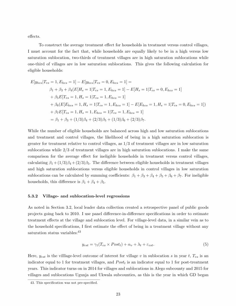
effects.

To construct the average treatment effect for households in treatment versus control villages,

I must account for the fact that, while households are equally likely to be in a high versus low

saturation sublocation, two-thirds of treatment villages are in high saturation sublocations while

one-third of villages are in low saturation sublocations. This gives the following calculation for

eligible households:

E[yhvs|Tvs = 1, Ehvs = 1]− E[yhvs|Tvs = 0, Ehvs = 1] =

β1 + β3 + β4(E[Hs = 1|Tvs = 1, Ehvs = 1]− E[Hs = 1|Tvs = 0, Ehvs = 1]

+ β5E[Tvs = 1, Hs = 1|Tvs = 1, Ehvs = 1]

+ β6(E[Ehvs = 1, Hs = 1|Tvs = 1, Ehvs = 1]− E[Ehvs = 1, Hs = 1|Tvs = 0, Ehvs = 1])

+ β7E[Tvs = 1, Hs = 1, Ehvs = 1|Tvs = 1, Ehvs = 1]

= β1 + β3 + (1/3)β4 + (2/3)β5 + (1/3)β6 + (2/3)β7.

While the number of eligible households are balanced across high and low saturation sublocations

and treatment and control villages, the likelihood of being in a high saturation sublocation is

greater for treatment relative to control villages, as 1/3 of treatment villages are in low saturation

sublocations while 2/3 of treatment villages are in high saturation sublocations. I make the same

comparison for the average effect for ineligible households in treatment versus control villages,

calculating β1 +(1/3)β4 +(2/3)β5. The difference between eligible households in treatment villages

and high saturation sublocations versus eligible households in control villages in low saturation

sublocations can be calculated by summing coefficients: β1 + β3 + β4 + β5 + β6 + β7. For ineligible

households, this difference is β1 + β4 + β5.

5.3.2 Village- and sublocation-level regressions

As noted in Section 3.2, local leader data collection created a retrospective panel of public goods

projects going back to 2010. I use panel difference-in-difference specifications in order to estimate

treatment effects at the village and sublocation level. For village-level data, in a similar vein as to

the household specifications, I first estimate the effect of being in a treatment village without any

saturation status variables:43

yvst = γ1(Tvs × Postt) + αv + λt + εvst. (5)

Here, yvst is the villlage-level outcome of interest for village v in sublocation s in year t, Tvs is an

indicator equal to 1 for treatment villages, and Postt is an indicator equal to 1 for post-treatment

years. This indicator turns on in 2014 for villages and sublocations in Alego subcounty and 2015 for

villages and sublocations Ugunja and Ukwala subcounties, as this is the year in which GD began

43. This specification was not pre-specified.

23

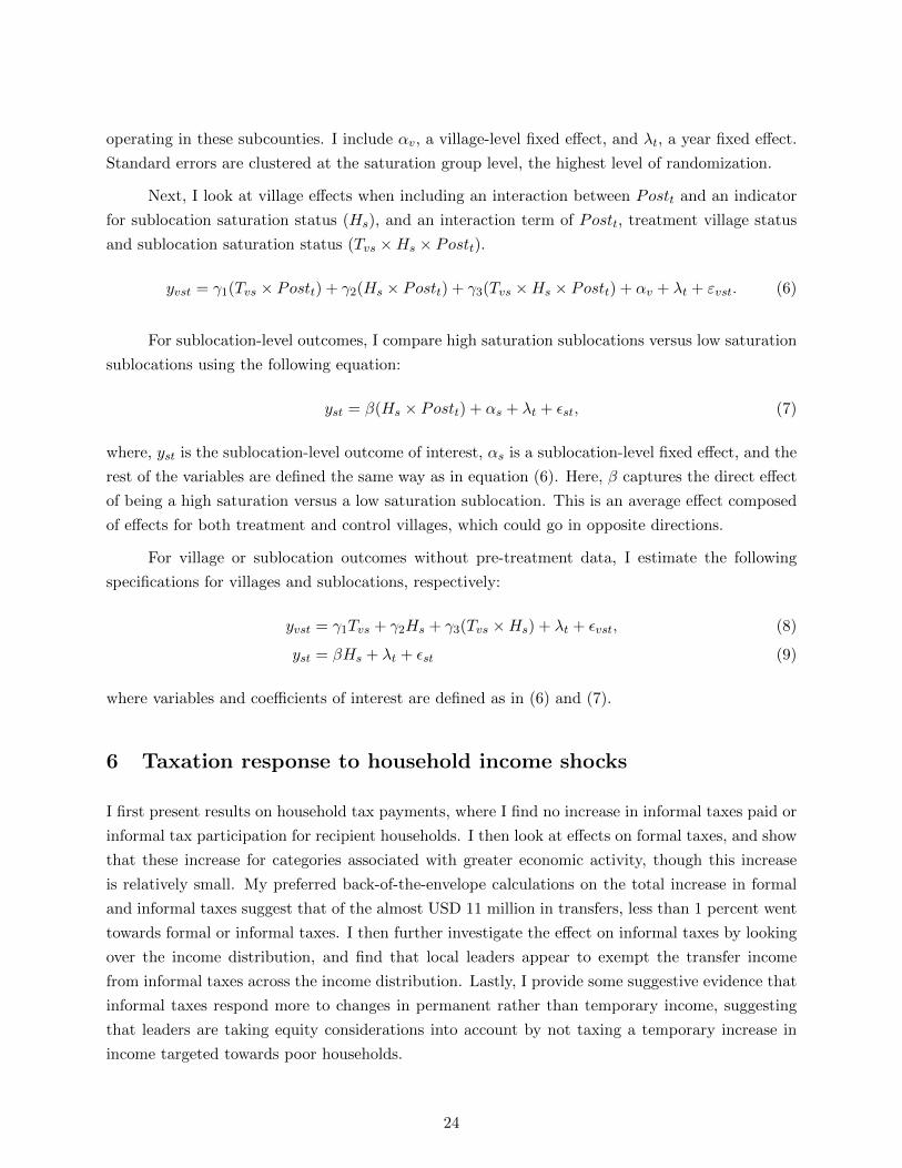
operating in these subcounties. I include αv, a village-level fixed effect, and λt, a year fixed effect.

Standard errors are clustered at the saturation group level, the highest level of randomization.

Next, I look at village effects when including an interaction between Postt and an indicator

for sublocation saturation status (Hs), and an interaction term of Postt, treatment village status

and sublocation saturation status (Tvs ×Hs × Postt).

yvst = γ1(Tvs × Postt) + γ2(Hs × Postt) + γ3(Tvs ×Hs × Postt) + αv + λt + εvst. (6)

For sublocation-level outcomes, I compare high saturation sublocations versus low saturation

sublocations using the following equation:

yst = β(Hs × Postt) + αs + λt + εst, (7)

where, yst is the sublocation-level outcome of interest, αs is a sublocation-level fixed effect, and the

rest of the variables are defined the same way as in equation (6). Here, β captures the direct effect

of being a high saturation versus a low saturation sublocation. This is an average effect composed

of effects for both treatment and control villages, which could go in opposite directions.

For village or sublocation outcomes without pre-treatment data, I estimate the following

specifications for villages and sublocations, respectively:

yvst = γ1Tvs + γ2Hs + γ3(Tvs ×Hs) + λt + εvst, (8)

yst = βHs + λt + εst (9)

where variables and coefficients of interest are defined as in (6) and (7).

6 Taxation response to household income shocks

I first present results on household tax payments, where I find no increase in informal taxes paid or

informal tax participation for recipient households. I then look at effects on formal taxes, and show

that these increase for categories associated with greater economic activity, though this increase

is relatively small. My preferred back-of-the-envelope calculations on the total increase in formal

and informal taxes suggest that of the almost USD 11 million in transfers, less than 1 percent went

towards formal or informal taxes. I then further investigate the effect on informal taxes by looking

over the income distribution, and find that local leaders appear to exempt the transfer income

from informal taxes across the income distribution. Lastly, I provide some suggestive evidence that

informal taxes respond more to changes in permanent rather than temporary income, suggesting

that leaders are taking equity considerations into account by not taxing a temporary increase in

income targeted towards poor households.

24

6.1 Household tax effects

I begin by looking at effects on informal taxes in terms of informal tax amounts, rates (as a share of

household income), participation (the extensive margin) and amount paid, conditional on making

any payment (the intensive margin). Table A.1 contains the full set of regression coefficients from

Equations (3) and (4).44 In Table 5, I highlight the main comparisons outlined above. The first

row presents the effect for an average household in a treatment versus control village, and reports

the result on the coefficient for being in a treatment village from Equation (3). The second and

third row use results from Equation (4) to calculate the mean effect of being an eligible and

ineligible household in a treatment versus control village, respectively. The fourth and fifth rows

also use coefficient estimates from Equation (4) but now to calculate the difference for eligible and

ineligible households in treatment villages in high saturation sublocations versus treatment villages

in low saturation sublocations. The results on formal taxes (broken down by county (primarily

self-employment) and national (primarily income) taxes follow the same format.

Table 5 shows there is no significant effects for the average, eligible or ineligible household

on the amount paid in formal taxes, the informal tax rate, nor the extensive or intensive margin.

While the point estimate for the amount of informal tax paid by eligible households is positive, the

upper bound of the 95 percent confidence interval (KES 53) corresponds to just 0.001 percent of the

total transfer amount. As discussed in Section 4, if the transfer income was taxed in the same way

as earned income, we would expect to see a similar change in magnitude as the number of income

deciles up the income distribution the transfer moves recipient households times the coefficient on

the change in informal taxes for a one decile shift in the income distribution, as reported in column

1 of Table 4. This estimated increase of KES 165 is much greater than the upper bound of the

95 percent confidence interval for the effect on total informal tax amount (KES 53). This strongly

suggests that transfer income is not being taxed in the same manner as earned income.

Next, I look at formal tax amounts, broken down by county taxes (primarily self-employment

taxes) and national taxes (primarily employee income taxes). While 15 percent of eligible house-

holds in control villages pay county taxes at endline, just 3 percent of households pay any national

taxes. In a similar manner to informal taxes, Table 6 presents the key comparisons of interest while

Table A.3 provides the full set of regression coefficients. Eligible households see an increase in

amount paid in county taxes. Column 3 of Table 6 shows this is driven in part by a 2.4 percentage

point increase in households paying any county taxes; the point estimate on amounts conditional on

any county tax payment for eligible households is positive but not statistically significant. Greater

county tax payment aligns with the fact that recipient households are more likely to be self-employed

(4 percentage points) as a result of the UCT.

I find a marginally significant effect for national taxes for ineligible households (Table 7),

driven by a large increase in the intensive margin. However, this appears likely to be a spurious

44. All tax amount values are topcoded at the 99th percentile; Appendix Table A.2 reproduces these results on theunwinsorized values.

25

correlation: the increase is driven by households in the top 1 percent of the income tax payment

distribution, which in this context is positions on the government payroll, such as teachers, which is

unlikely to be affected by cash transfers. I find no change in national taxes for eligible households.

In order to calculate a measure of the total estimated increase in taxes per household as a

result of the cash transfer payment, I take the point estimates for the tax effects for the mean

household in treatment villages seriously, regardless of statistical significance. This implies an

average increase of KES 145 (a KES 28 increase in informal taxes plus a KES 21 increase in county

taxes plus a KES 96 increase in national taxes). With an average of 100 households per village,

328 treatment villages in our study and an exchange rate of 100 KES to 1 USD, this corresponds

to a total tax increase of USD 47,560, or 0.4 percent of the total amount transferred by GD into

the study area. Focusing instead on the effects for informal and county taxes, which seem more

likely to be in response to the cash transfers, provides an estimate of 0.15 percent with winsorized

values from the main tables, or 0.53 percent with unwinsorized values (Appendix Tables A.2 and

A.4). Overall, the magnitude of any tax increases are small relative to the total transfer amount.

6.2 Recipient households pay informal taxes in line with baseline income

I now turn to investigate the lack of an effect on informal taxes in more detail. I test and strongly

reject that recipient households pay informal taxes on the basis of their annual income, inclusive

of the UCT transfer. I can also reject (at p=0.068) that recipient households are paying the same

amount of informal taxes as control households with similar amounts of earned income at endline.

However, recipient informal tax amounts are consistent with a tax schedule based on pre-transfer

income. I cannot reject (p=0.37) that recipient households are paying the same amount in informal

taxes as control households in the same baseline income decile. This suggests that local leaders

tax households based on their permanent income, rather than on their annual income, which may

include temporary shocks. I discuss the robustness of this finding to alternative interpretations in

Section 8.

I construct three measures of household income deciles: i) baseline earned income, ii) end-

line earned income, and iii) endline earned plus UCT transfer income. All endline income decile

thresholds are calculated based on control households and weighted to reflect population averages.

I then compare households in control villages to recipient households by regressing indicators for

each income decile, and interaction terms between recipient status and each income decile, on the

amount paid in informal taxes at endline:

InformalTaxhvstE =

10∑j=1

βj(INCDECmj × Tvs × Ehvs) +

10∑k=1

δkINCDECmk + εhvstE . (10)

InformalTaxhvstE denotes the endline informal tax amount paid by household h in village v in

sublocation s at endline (tE and tB denote baseline and endline survey rounds, respectively). As

26

above, Tvs is an indicator variable equal to one for households in treatment villages and Ehvs is an

indicator equal to one for eligible households, so the interaction term between these two variables

represents recipient households. INCDECmj represents the j-th income decile calculated via

method m, where m ∈ {Baseline income,Endline earned income,Endline earned income + UCT}.εhsvtE is an error term clustered at the village level.

The βj ’s are the coefficients of interest; I report these in table 8 and conduct a joint F-

test for whether all of the βj terms are equal to zero. I cannot reject that the interaction terms

between baseline income deciles and recipient households are jointly significant at a 10 percent

level (column 1), while I can strongly reject (p-value < 0.01) that the interaction terms for endline

income inclusive of the UCTs are jointly zero.45 I can reject that the βj coefficients are jointly

equal to zero for endline income deciles based on earned income at a 10 percent significance level.

When factoring in the UCT income, the point estimates for 7 of the 10 coefficients on income

deciles interacted with recipient status are negative. This implies that recipient households pay less

in informal taxes at endline than control households with similar endline income, Instead, recipient

households pay tax amounts comparable to other control households with the same baseline income.

Next, I calculate a counterfactual amount that recipient households would have paid if they

paid informal taxes based on their annual income. I calculate baseline income deciles without the

transfer income, then add the transfer amount and calculate where recipient households now fall.

We would expect to see recipient households paying amounts similar to control group households

in the top decile, as the transfer income shifts all recipient households to the top decile. This may

overstate the shift up the income distribution for recipient households if income is underreported.

Figure 3 displays this shift in the income distribution graphically.

Next, I calculate the amount of endline informal taxes paid by control households by baseline

income decile as the counterfactual informal tax schedule.46 The gray line in Figure 6 plots this

schedule. As all recipient households move up to the top decile, if they were taxed in the same way

as control households with similar baseline income, recipient households would pay the same amount

as control households in the top decile. The dotted line in Figure 6 plots this counterfactual tax

rate for recipient households based on the progressivity of the control household schedule. Lastly, I

plot the actual amount paid by recipient households at endline by their pre-transfer baseline income

in the solid black line. I cannot reject that recipient households pay the same amount in informal

taxes at endline by income decile as control households.47

Here again, across income deciles, we see that recipient households are being taxed similarly

45. These results include conservative assumptions about the distribution of UCT transfers and their implicationsfor household income. I assign UCT transfer income to households on the basis of their villages experimental startdate, and assume that all households within the village began receiving UCTs in the experimental start month.This frontloads the distribution of UCTs to households and thus reduces the amount of transfer income I assign tohouseholds as being distributed in the last 12 months.

46. Here, and in what follows, I weight households by the inverse share surveyed per village by eligibility statuswhen constructing deciles, and report unweighted values when calculating outcomes by or conditional on deciles.

47. I test this using Equation (10). The point estimates in column 1 match the difference between the two lines.

27

to their baseline income, rather than what they would have been paying based on their shift up

the income distribution. This is especially pronounced for households at the lowest income deciles.

Notably, we also see that households with higher pre-treatment incomes (those in the top deciles

of the baseline income distribution) are also not paying more than control households in the top

baseline income deciles. Likewise, recipient households in the 9th and 10th baseline wealth deciles

also do not pay more in endline informal taxes (Appendix Table A.7). These households are the

ones with the greatest relative ability to pay in response to an exogenous income shock, and yet

they still pay no more in taxes than control group households in the same baseline decile.

I then look at specific types of income changes that are more likely to reflect changes in

permanent income, and investigate how household informal tax rates change in response to these

income changes. While agricultural income may be driven by weather shocks and thus more tempo-

rary, changes in the amount of land used for agriculture is more likely to be associated with changes

in one’s permanent agricultural income. I calculate the change in agricultural land used at endline

relative to baseline, and generate an indicator for households that increase their agricultural land

and an indicator for households that decrease their agricultural land. I also generate indicators

for households that report having started a new job since the date of the household’s baseline

survey (in both cases, these could either be the household’s first enterprise/job or an additional

enterprise/job). Lastly, I use village elder reports of whether the village experienced too much or

too little rain in 2016 (which corresponds to the main harvest season for households at endline) as

a measure of temporary income shocks. While this is not a perfect measure since it is at the village

level, it can be useful in providing a comparison to the magnitudes of the more permanent income

changes.

I estimate

∆InformalTaxhvs = β0 + β1Xhvs + εhvs, (11)

where standard errors are clustered at the village level. Table 9 presents the results. In columns

1 through 4, I include only non-recipient households, and include an indicator for whether these

households are in treatment villages.48 Column 1 estimates changes in informal taxes as a function

of changes in income deciles (as in Table 4) for this sample as a reference. Column 2 includes the

indicator variables associated with changes in permanent income. The signs on all coefficients go

in the expected direction: increasing agricultural land and starting a job are all associated with an

increase in informal taxes. I next introduce an indicator for a village-level rainfall shock in column

3, and, as expected, it enters negatively. The magnitude of this temporary negative income shock is

half as large as the magnitude of the more permanent shock of reducing the amount of agricultural

land used. In column 4, I estimate both the permanent and temporary shocks together, and the

results are similar, with all coefficients going in the expected direction. Lastly, I use all panel

households and introduce indicators for eligibility status and recipients (the interaction between

48. Note that I do not find a significant effect for ineligible households in treatment versus control villages on theseoutcomes (not shown).

28

treatment village and eligibility status), and find that the magnitude of the effect on the temporary

income shock associated with receiving a transfer is about 1/3 as large as the effect of the rainfall

shock, and not statistically significant.

Taken together, this provides some suggestive evidence that the transfer income may be

exempt due to the fact that it is a temporary, rather than a permanent shock. This highlights

a potential benefit of informal taxation relative for formal taxation in an environment with high

income volatility. In many developed country tax systems (such as the US), one-time income

shocks such as gambling or lottery winnings are subject to taxation and count as income towards

a household’s tax base, regardless of the household’s earned income. The discretion offered by

informal taxation allows leaders to avoid overtaxing households with less lifetime earnings ability

than their annual income would otherwise suggest. I discuss the robustness of this implication to

alternative mechanisms in more detail in Section 8.

7 Public goods effects

I next turn my attention to whether there is an increase in a) the number of public goods projects

and b) reported public goods quality. Focusing on the number of projects offers an advantage in

that local leaders are more likely to recall projects, even when they do not recall specific amounts,

though this does not capture different project scales.49 Public goods projects are defined as either

new constructions, improvements or repairs, and exclude regular upkeep such as cleaning. Examples

of projects present in my data include installing a chlorine dispenser at a water point, protecting

a spring, fencing a school, and grading a feeder road. As shown in Figure 2, the cost and scope

of projects can vary, in part depending on whether villages receive any project funding from the

national or county government, yet there are many smaller projects undertaken by villages without

external funding. For instance, 2 percent of the mean village-level transfer amount would cover the

cost of protecting a spring.

At the village level, I calculate the overall number of projects, which sums water point

projects, feeder road and bridge projects, and projects at other village-level facilities. I then look

specifically at water points and feeder road and bridge projects due to the fact that both of these

facilities are ubiquitous: 99 percent of villages have at least one water point (with a mean of 3.6)

and 95 percent of villages have at least one feeder road (with a mean of 2.3). At the sublocation

level, I look at the overall number of projects, which sums the number of health clinic projects,

market center projects, and other sublocation-level projects. As not all sublocations have these

public facilities, sublocation outcome variables are conditional on the presence of a public facility.

Table 10 presents results at the village level on the number of public goods projects (columns

1 through 4) and public goods quality (columns 5 through 8). Perhaps unsurprisingly given the

49. In appendix table A.9 I show that there is also no effect on reported public goods expenditures, though asnoted, for approximately 20 percent of projects leaders report that they do not know the spending amount.

29

lack of effects on informal taxation, there is no effect on these categories of public goods projects.

Villages in high-saturation sublocations report an increase in the number of projects due to an

increase in water point projects post-treatment, but this is not driven by treatment villages in

high-saturation areas, nor by projects that involve local (village) funds. Villages in high-saturation

areas are 6.4 percentage points more likely to receive NGO funding (p-value 0.025), suggesting this

increase may be driven by other NGO activity rather than a response to cash transfers.

I next turn to the quality of public goods reported by village elders and households. For all

questions, I code responses of very good as 5, good as 4, fair as 3, poor as 2, and very poor as 1,

so that higher values correspond to better-quality public goods. Questions on the quality of public

goods were only included in the endline household survey and second round of local leader surveys.

For households, I estimate equations (3) and (4) without baseline values of the outcome variable;

for village elders I use equations (8). For households and village elders, I construct a mean effects

index of standardized variables following Kling, Liebman, and Katz (2007) as an overall measure

of public goods quality for each household/village, and also report results from each component.

The household index is an index of reported quality of water points, feeder roads and bridges, and

health clinics facing the household. Village elders were asked about the quality of each public good

within their village; I use the mean value of water points and road/bridge quality, given that almost

all villages have these. If a village does not have a water point or road/bridge, I code this as zero.50

Table 10, columns 5 through 8 presents results on public goods quality, village elders (columns

5 and 6), eligible households (column 7) and ineligible households (column 8).I find no statistically

significant effects for treatment villages, eligible or ineligible households, and coefficient estimates

are small in magnitude. Consistent with the increase in the number of water point projects in high-

saturation sublocations, village elders in high-saturation sublocations report a significant increase

in water point quality. As noted above, this appears driven by an increase in NGO activity, and

this increase is not echoed by households. Overall, these results suggest no increase in the quality

of public goods.

Taken together, these results suggest that the unconditional cash transfers had no short-run

effects on local public goods. It is important to note that there does not appear to be a negative

effect on public goods, as could occur if villages that did not receive cash transfers were targeted for

greater development expenditure at the expense of treatment villages. The tradeoff to exempting

UCT income is that leaders forgo potential informal tax revenue and the associated public goods

development that could accompany this. If the UCT amount was taxed at the average informal

tax rate for eligible households in control villages (1.9 percent), the mean village would raise an

additional USD 545 in informal tax revenue, roughly the same amount as it would cost to protect

a spring. As an alternative measure based on marginal taxes, I calculate the “revenue gap” as the

50. Appendix Table A.8, columns 5 and 6 reports assistant chief responses to questions on the quality of healthclinics and market centers. I do not create an index of sublocation-level projects due to the fact that not everysublocation will have a health clinic and market center. Instead, I look at sublocation-level outcomes on healthclinics and market centers for the sublocations that have these facilities.

30

difference between the counterfactual tax amount recipient households would pay, and the actual

amount paid by recipient households (the difference between the dotted line and the solid black line

in Figure 6). I multiply this by the number of recipient households in each income decile, scaling

these up to represent the total number of recipient households in the study area, and divide by the

number of treatment villages. Based on this calculation, the mean village would have an additional

KES 5,105 to spend on public goods development. This is over 30 percent of the mean annual

expenditure from local sources for water points, and the median water point project cost KES

8,000 (Figure 2). Interestingly, informal taxes at the top decile were higher at baseline relative to

endline. Using the amount paid by the top income decile at baseline gives an estimate of a revenue

gain of KES 14,300, or nearly 100 percent of the mean annual local expenditure per village on

water points.

8 Discussion

In order for leaders to make a tradeoff between exempting poor recipient households from taxes

and public goods, leaders must be aware of the households receiving the transfers. The fact the

transfer is distributed via mobile money could make it harder for leaders to know when (and what)

households are receiving transfers. However, as previously noted, the NGO informed leaders and

held a village meeting prior to beginning work within a village. The means-test eligibility criteria

are publicly observable and easy to discern.51 In addition, many recipient households spent the

transfers on observable goods: there is a 40 percentage point increase in the share of households

with metal roofs.52 This type of spending would be a further signal to leaders of households’

status. What is more, transfers were distributed at roughly the same time to all households within

a village, so if a leader could determine when one household was receiving transfers, s/he would be

well-informed about the timing of the transfer for other households as well. Taken together, this

suggests lack of awareness is unlikely to explain the null effects on informal taxes. However, my

findings are also consistent with low-capacity local leaders.

Another alternative reason why we might not see an change in informal taxes from baseline

income levels is if informal taxes are fixed per-household and not subject to change. However, as

previously shown in Table 4, informal taxes do respond to changes in income for control group

households. Table 4 shows that shifting up one income decile is associated with an increase of

KES 33 in informal taxes; the point estimate of KES 14 for eligible households in treatment versus

control villages from the main household tax results in Table 5 is consistent with households moving

up less than one income decile. In addition, even though there is no change in the overall informal

51. For example, the author accompanied fieldworkers with the NGO on a census visit to a household with a metalroof; the resident consented to the census but informed the NGO staff that she knew she would not be receiving atransfer due to her metal roof.

52. However, spending on observables could be a signal to leaders that the household has already spent the transferand no longer has cash on hand.

31

tax participation rate for eligible or ineligible households, there is substantial movement on the

extensive margin across years: 36 percent of households do not pay any informal taxes at either

baseline or endline, 23 percent of households pay informal taxes at both baseline and endline, and

40 percent of households pay any informal taxes either at baseline or endline but not both.

The fact informal taxes do change for households over time, and in response to more per-

manent changes in household income, also means that potential alternative drivers of informal tax

levels must also change with income. For instance, if informal taxes are assessed on the basis of so-

cial status rather than income, changes in permanent income must also be associated with changes

in social status significant enough to cause changes in household informal tax obligations. However,

I cannot fully rule out that another factor may be driving the relationship between income, wealth

and informal taxes for public goods spending that may not be changed by the receiving a cash

transfer.

If there are no investment opportunities for which the marginal social benefit is greater than

the marginal social cost even after the transfers, then we would not expect to see an increase in

public goods provision, nor an increase in total informal tax revenue collected by local leaders.

However, it is generally thought that there is under-provision of public goods in rural settings in

developing countries; rural Kenya is no exception. In endline household surveys, households were

asked how they would spend KES 50,000 on a development project of their choice, and read a list of

options, including “no need for more development”. Less than 1 percent of households responded

there was no need for more development. While this is not a revealed preference or contingent

valuation estimate, and does not require potential contribution from household, it is consistent

with a desire for increased public goods projects on the part of households. Figure 2 shows that

many projects are small. Given the large magnitude of the transfers, even 1 to 2 percent of transfer

amount would cover the cost of a number of types of projects. This suggests that there is scope to

raise sufficient funding to carry out projects.

The exogenous income shock could change household attitudes in a way that makes it more

difficult for leaders to collect informal taxes. I do not find significant changes in an index on

household support for redistribution, nor on measures of social trust and cohesion (Table 11).

Support for redistribution by local leaders within the village is high, but there is no difference

between treatment and control villages. I do find that recipient households are somewhat less

likely to support a progressive tax schedule. There is no reported change for eligible or ineligible

households in whether they can trust members of their own villages. Recipient households also

increase their membership in community groups. This is suggestive that the capacity to organize

and undertake community projects has not substantially changed, and that recipient households

are not opting out of community institutions after receiving the transfer.

I also cannot rule out that these effects are unique to changes in income due to NGO de-

velopment assistance, or a feature of this particular cash transfer program. GD emphasized that

households receiving the UCT were not selected by the government or by local leaders, which could

32

have limited the ability of leaders to enforce collections.

9 Conclusion

I use detailed original panel data from households and local leaders to study informal taxation and

public goods provision. I document that informal taxes are widespread, are increasing in income

but regressive and make up an important component of village funding for public goods, consistent

with cross-sectional findings by Olken and Singhal (2011). I then utilize the panel nature of my

data to show informal taxes respond to changes in earned income and wealth. This appears to be

especially true for changes related to permanent income, such as starting a new job or changing the

amount of agricultural land under cultivation. This is suggestive that leaders are basing informal

taxes on income, as an alternative driver (such as social standing) would have to co-move with both

income and informal taxes.

In response to a large distribution of one-time, unconditional cash transfers to poor households

in Kenya, I find no increase in informal tax payments for either recipient or non-recipient households.

This is despite local leaders being knowledgable of the transfers, and with transfers distributed

concurrently within a village. I reject the null hypothesis that household informal taxes are based

on annual income, and instead find evidence consistent with informal taxes for recipient households

being based on their pre-treatment income levels. This is consistent with local leaders exempting

temporary income shocks (especially to poor households) and taxing households on the basis of

their baseline income rather than their earned income inclusive of the transfer amount. In a

setting where the central government has little verifiable information about households’ income,

the flexible nature of informal taxes allows for leader discretion in taking factors outside of income

into account when setting taxes. This highlights an under-appreciated benefit of informal taxes in

an environment with high income volatility.

However, exempting these large temporary income shocks to poor households trades off a

potentially sizable increase in informal tax revenue that could go towards additional public goods

projects. As in many settings in low-income countries, there is substantial scope to improve public

infrastructure, in particular water infrastructure, at relatively low cost while reaping potentially

large health benefits. I find no evidence of effects on the number of public goods projects or quality,

both overall and on water points in particular. If tax increases are tied to changes in permanent

income (rather than temporary income shocks), this suggests that sustained income growth is

required in order for local communities to undertake public goods projects themselves. In the

Kenyan context, formal government development expenditure (such as from politician-controlled

development funds) may be better placed to fund public goods.

While this suggests limited effects of unconditional cash transfers on taxation and public

goods, this does not negate the positive benefits to recipient households documented here and in

the literature. It also shows that local leaders are not overtaxing recipient households, limiting

33

concerns about elite capture of the transfer income and providing evidence that the bulk of the

cash transfers are reaching their intended target of poor households. These findings are especially

relevant for policy as UCT programs continue to expand.

34

References

Acemoglu, Daron, Tristan Reed, and James A. Robinson. 2014. “Chiefs: Economic Development

and Elite Control of Civil Society in Sierra Leone.” Journal of Political Economy (2): 319–368.

Alatas, Vivi, Abhijit Banerjee, Rema Hanna, Benjamin A. Olken, and Julia Tobias. 2012. “Targeting

the Poor: Evidence from a Field Experiment in Indonesia.” American Economic Review 102,

no. 4 (June): 1206–40.

Arnold, Catherine, Tim Conway, and Michael Greenslade. 2011. “Cash Transfers.” DFID Evidence

Paper.

Baldwin, Kate. 2016. The Paradox of Traditional Chiefs in Democratic Africa. New York: Cam-

bridge University Press.

Barkan, J, and F Holmquist. 1986. “Politics and the Peasantry in Kenya: The Lessons of Harambee.”

Institute for Development Studies, University of Nairobi, Working paper No.440.

Bastagli, Francesca, Jessica Hagen-Zanker, Luke Harman, Valentina Barca, Georgina Sturge, and

Tanja Schmidt with Luca Pellerano. 2016. Cash transfers: what does the evidence say? A

rigorous review of programme impact and of the role of design and implementation features.

Overseas Development Institute, July.

Besley, Timothy, and Torsten Persson. 2013. “Taxation and Development.” In Handbook of Public

Economics, edited by Alan Auerbach, Raj Chetty, Martin Feldstein, and Emmanuel Saez,

5:51–110. Amsterdam: Elsevier.

DFID. 2013. “Taxation and livelihoods: evidence from fragile and conflict-affected situations.” DFID

Evidence Brief, October.

Evans, David K., and Anna Popova. 2014. “Cash Transfers and Temptation Goods: A Review of

Global Evidence.” World Bank Policy Research Working Paper 6886, May.

Faye, Michael, Paul Niehaus, and Chris Blattman. 2015. “Worth Every Cent: To Help the Poor,

Give them Cash.” Foreign Affairs (October).

Gardner, Leigh A. 2010. “Decentralization and Corruption in Historical Perspective: Evidence from

Tax Collection in British Colonial Africa.” Economic History of Developing Regions 25 (2):

213–236.

Haushofer, Johannes, Edward Miguel, Paul Niehaus, and Michael Walker. 2014. “General Equi-

librium Effects of Cash Transfers in Kenya.” AEA Trial Registry. November. https://www.

socialscienceregistry.org/trials/505/history/3031.

. 2016. “Pre-analysis Plan for Midline Data: General Equilibrium Effects of Cash Transfers.”

May.

35

Haushofer, Johannes, Paul Niehaus, Edward Miguel, and Michael Walker. 2017. “Household Welfare

Effects of Cash Transfers: Evidence from a Large-Scale RCT in Kenya.” In preparation.

Haushofer, Johannes, and Jeremy Shapiro. 2016. “The Short-Term Impact of Unconditional Cash

Transfers to the Poor: Experimental Evidence from Kenya.” The Quarterly Journal of Eco-

nomics 131 (4): 1973–2042.

Jack, William, and Tavneet Suri. 2011. “Mobile Money: The Economics of M-PESA.” NBER Work-

ing Paper No. 16721, January.

Jakiela, Pamela, and Owen Ozier. 2016. “Does Africa Need a Rotten Kin Theorem? Experimental

Evidence from Village Economies.” Review of Economic Studies (1): 231–268.

Khan, Adnan, Asim Khwaja, and Benjamin Olken. 2016. “Tax Farming Redux: Experimental

Evidence on Performance Pay for Tax Collectors,” 131 (1): 219–271.

Kleven, Henrik Jacobsen, Claus Thustrup Kreiner, and Emmanuel Saez. 2009. “Why Can Modern

Governments Tax So Much? An Agency Model of Firms as Fiscal Intermediaries.” NBER

Working Paper No. 15218, August.

Kling, Jeffrey R, Jeffrey B Liebman, and Lawrence F Katz. 2007. “Experimental Analysis of Neigh-

borhood Effects.” Econometrica 75 (1): 83–119.

Kremer, Michael, Jessica Leino, Edward Miguel, and Alix Peterson Zwane. 2011. “Spring Clean-

ing: Rural Water Impacts, Valuation, and Property Rights Institutions.” Quarterly Journal of

Economics 126 (1): 145–205.

Margolies, Amy, and John Hoddinott. 2015. “Costing alternative transfer modalities.” Journal of

Development Effectiveness 7 (1): 1–16.

Mbiti, Isaac, and David N. Weil. 2015. “Mobile Banking: The Impact of M-Pesa in Kenya.” In

African Successes, Volume III: Modernization and Development, 247–293. NBER Chapters.

National Bureau of Economic Research, Inc, March.

McKenzie, David. 2012. “Beyond baseline and follow-up: The case for more T in experiments.”

Journal of Development Economics 99 (2): 210–221.

Miguel, Edward, and Mary Kay Gugerty. 2005. “Ethnic diversity, social sanctions, and public goods

in Kenya.” Journal of Public Economics 89, nos. 11-12 (December): 2325–2368.

Munshi, Kaivan, and Mark Rosenzweig. 2015. “Insiders and Outsiders: Local Ethnic Politics and

Public Goods Provision.” November.

Ngau, Peter M. 1987. “Tensions in Empowerment: The Experience of the Harambee (Self-Help)

Movement in Kenya.” Economic Development and Cultural Change 35 (3): 523–38.

36

Olken, Benjamin A., and Monica Singhal. 2011. “Informal Taxation.” American Economic Journal:

Applied Economics 3, no. 4 (October): 1–28.

Squires, Munir. 2017. “Kinship Taxation as an Impediment to Growth: Experimental Evidence

from Kenyan Microenterprises.” Working paper.

Udry, Christopher. 1994. “Risk and Insurance in a Rural Credit Market: An Empirical Investigation

in Northern Nigeria” [in English]. The Review of Economic Studies 61 (3): 495–526.

Walker, Michael. 2017. “Pre-Analysis Plan: Local Public Finance and Unconditional Cash Transfers

in Kenya.” February.

Zhang, Kelly. 2017. “Corrupting Politicians: Evidence from Kenya.” Unpublished doctoral thesis,

Stanford University.

37

10 Tables and Figures

38

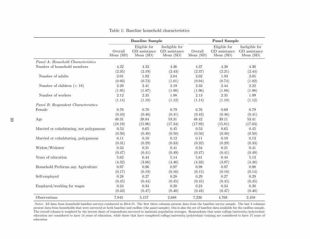
Table 1: Baseline household characteristics

Baseline Sample Panel Sample

OverallMean (SD)

Eligible forGD assistance

Mean (SD)

Ineligible forGD assistance

Mean (SD)Overall

Mean (SD)

Eligible forGD assistance

Mean (SD)

Ineligible forGD assistance

Mean (SD)

Panel A: Household CharacteristicsNumber of household members 4.32 4.33 4.26 4.37 4.38 4.30

(2.35) (2.19) (2.43) (2.37) (2.21) (2.44)Number of adults 2.01 1.92 2.04 2.02 1.93 2.05

(0.93) (0.73) (1.01) (0.94) (0.74) (1.02)Number of children (< 18) 2.29 2.41 2.19 2.33 2.44 2.22

(1.95) (1.87) (1.98) (1.96) (1.88) (1.98)Number of workers 2.12 2.35 1.98 2.13 2.35 1.99

(1.14) (1.10) (1.12) (1.14) (1.10) (1.12)Panel B: Respondent CharacteristicsFemale 0.76 0.70 0.79 0.76 0.69 0.79

(0.43) (0.46) (0.41) (0.43) (0.46) (0.41)Age 48.31 38.84 53.31 48.42 39.11 53.41

(18.19) (15.96) (17.34) (17.92) (15.81) (17.03)Married or cohabitating, not polygamous 0.53 0.65 0.45 0.53 0.65 0.45

(0.50) (0.48) (0.50) (0.50) (0.48) (0.50)Married or cohabitating, polygamous 0.11 0.10 0.12 0.11 0.10 0.13

(0.31) (0.29) (0.33) (0.32) (0.29) (0.33)Widow/Widower 0.34 0.21 0.41 0.34 0.21 0.41

(0.47) (0.41) (0.49) (0.47) (0.41) (0.49)Years of education 5.62 6.44 5.14 5.61 6.44 5.13

(4.32) (3.86) (4.46) (4.33) (3.87) (4.48)Household Performs any Agriculture 0.97 0.96 0.97 0.98 0.97 0.98

(0.17) (0.19) (0.16) (0.15) (0.18) (0.14)Self-employed 0.28 0.27 0.28 0.29 0.27 0.29

(0.45) (0.44) (0.45) (0.45) (0.45) (0.45)Employed/working for wages 0.24 0.34 0.20 0.24 0.34 0.20

(0.43) (0.47) (0.40) (0.43) (0.47) (0.40)

Observations 7,845 5,157 2,688 7,226 4,768 2,458

Notes: All data from household baseline surveys conducted in 2014-15. The first three columns present data from the baseline survey sample. The last 3 columnspresent data from households that were surveyed at both baseline and endline (the panel sample); this is also the set of baseline data available for the endline sample.The overall column is weighted by the inverse share of respondents surveyed to maintain population averages. Respondents that some college/university/polytechniceducation are considered to have 14 years of education, while those that have completed college/university/polytechnic training are considered to have 15 years ofeducation

39

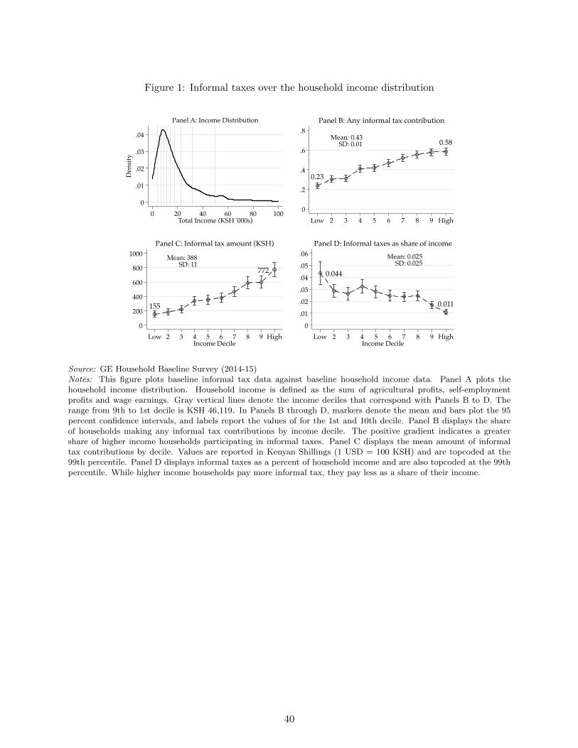
Figure 1: Informal taxes over the household income distribution

0

.01

.02

.03

.04D

ensi

ty

0 20 40 60 80 100Total Income (KSH '000s)

Panel A: Income Distribution

0.23

0.58Mean: 0.43

SD: 0.01

0

.2

.4

.6

.8

Low 2 3 4 5 6 7 8 9 High

Panel B: Any informal tax contribution

155

772

Mean: 388SD: 11

0

200

400

600

800

1000

Low 2 3 4 5 6 7 8 9 HighIncome Decile

Panel C: Informal tax amount (KSH)

0.044

0.011

Mean: 0.025SD: 0.025

0

.01

.02

.03

.04

.05

.06

Low 2 3 4 5 6 7 8 9 HighIncome Decile

Panel D: Informal taxes as share of income

Source: GE Household Baseline Survey (2014-15)Notes: This figure plots baseline informal tax data against baseline household income data. Panel A plots thehousehold income distribution. Household income is defined as the sum of agricultural profits, self-employmentprofits and wage earnings. Gray vertical lines denote the income deciles that correspond with Panels B to D. Therange from 9th to 1st decile is KSH 46,119. In Panels B through D, markers denote the mean and bars plot the 95percent confidence intervals, and labels report the values of for the 1st and 10th decile. Panel B displays the shareof households making any informal tax contributions by income decile. The positive gradient indicates a greatershare of higher income households participating in informal taxes. Panel C displays the mean amount of informaltax contributions by decile. Values are reported in Kenyan Shillings (1 USD = 100 KSH) and are topcoded at the99th percentile. Panel D displays informal taxes as a percent of household income and are also topcoded at the 99thpercentile. While higher income households pay more informal tax, they pay less as a share of their income.

40

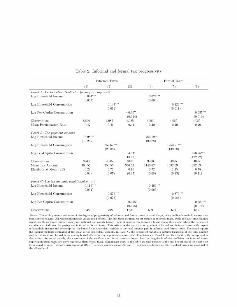
Table 2: Informal and formal tax progressivity

Informal Taxes Formal Taxes

(1) (2) (3) (4) (5) (6)

Panel A: Participation (Indicator for any tax payment)Log Household Income 0.044∗∗∗ 0.074∗∗∗

(0.007) (0.006)Log Household Consumption 0.147∗∗∗ 0.120∗∗∗

(0.014) (0.011)Log Per-Capita Consumption −0.007 0.055∗∗∗

(0.014) (0.010)Observations 3,860 4,085 4,085 3,860 4,085 4,085Mean Participation Rate 0.42 0.41 0.41 0.20 0.20 0.20

Panel B: Tax payment amountLog Household Income 75.98∗∗∗ 783.79∗∗∗

(12.29) (90.88)Log Household Consumption 252.67∗∗∗ 1253.51∗∗∗

(23.89) (139.88)Log Per-Capita Consumption 34.81∗ 850.25∗∗∗

(18.02) (122.22)Observations 3860 4085 4085 3860 4085 4085Mean Tax Amount 360.55 350.53 350.53 1146.62 1092.09 1092.09Elasticity at Mean (SE) 0.22 0.72 0.10 0.72 1.15 0.78

(0.04) (0.07) (0.05) (0.08) (0.13) (0.11)

Panel C: Log tax amount, conditional on > 0Log Household Income 0.119∗∗∗ 0.469∗∗∗

(0.034) (0.066)Log Household Consumption 0.579∗∗∗ 0.870∗∗∗

(0.073) (0.086)Log Per-Capita Consumption 0.095∗ 0.584∗∗∗

(0.055) (0.070)Observations 1638 1708 1708 639 659 659

Notes: This table presents estimates of the degree of progressivity of informal and formal taxes in rural Kenya, using endline household survey datafrom control villages. All regressions include village fixed effects. The first three columns report results on informal taxes, while the last three columnsreport results on direct formal taxes (both national and county taxes). Panel A reports results from a linear probability model where the dependentvariable is an indicator for paying any informal or formal taxes. This estimates the participation gradient of formal and informal taxes with respectto household income and consumption. In Panel B the dependent variable is the total amount paid in informal and formal taxes. The panel reportsthe implied elasticity evaluated at the mean of the dependent variable. In Panel C, the dependent variable is natural logarithm of the total amountpaid in informal and formal taxes among households reporting a positive amount paid. Coefficients in Panel C can thus be directly interpreted aselasticities. Across all panels, the magnitude of the coefficient on formal taxes is larger than the magnitude of the coefficient on informal taxes,implying informal taxes are more regressive than formal taxes. Significance stars in the table are with respect to the null hypothesis of the coefficientbeing equal to zero. * denotes significance at 10%, ** denotes significance at 5%, and *** denotes significance at 1%. Standard errors are clustered atthe village level.

41

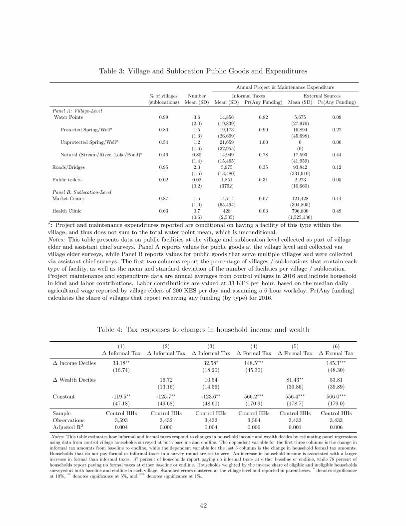
Table 3: Village and Sublocation Public Goods and Expenditures

Annual Project & Maintenance Expenditure

% of villages Number Informal Taxes External Sources(sublocations) Mean (SD) Mean (SD) Pr(Any Funding) Mean (SD) Pr(Any Funding)

Panel A: Village-LevelWater Points 0.99 3.6 14,856 0.82 5,675 0.09

(2.0) (19,839) (27,976)Protected Spring/Wella 0.80 1.5 19,173 0.90 16,894 0.27

(1.3) (26,699) (45,698)Unprotected Spring/Wella 0.54 1.2 21,659 1.00 0 0.00

(1.6) (22,955) (0)Natural (Stream/River, Lake/Pond)a 0.46 0.80 14,949 0.78 17,593 0.44

(1.4) (15,465) (41,959)Roads/Bridges 0.95 2.3 5,975 0.35 93,842 0.12

(1.5) (13,480) (331,910)Public toilets 0.02 0.02 1,851 0.31 2,273 0.05

(0.2) (3792) (10,660)Panel B: Sublocation-LevelMarket Center 0.87 1.5 14,714 0.07 121,428 0.14

(1.0) (65,494) (394,805)Health Clinic 0.63 0.7 428 0.03 796,800 0.49

(0.6) (2,535) (1,525,136)a: Project and maintenance expenditures reported are conditional on having a facility of this type within thevillage, and thus does not sum to the total water point mean, which is unconditional.Notes: This table presents data on public facilities at the village and sublocation level collected as part of villageelder and assistant chief surveys. Panel A reports values for public goods at the village level and collected viavillage elder surveys, while Panel B reports values for public goods that serve multiple villages and were collectedvia assistant chief surveys. The first two columns report the percentage of villages / sublocations that contain eachtype of facility, as well as the mean and standard deviation of the number of facilities per village / sublocation.Project maintenance and expenditure data are annual averages from control villages in 2016 and include householdin-kind and labor contributions. Labor contributions are valued at 33 KES per hour, based on the median dailyagricultural wage reported by village elders of 200 KES per day and assuming a 6 hour workday. Pr(Any funding)calculates the share of villages that report receiving any funding (by type) for 2016.

Table 4: Tax responses to changes in household income and wealth

(1) (2) (3) (4) (5) (6)∆ Informal Tax ∆ Informal Tax ∆ Informal Tax ∆ Formal Tax ∆ Formal Tax ∆ Formal Tax

∆ Income Deciles 33.18∗∗ 32.58∗ 148.5∗∗∗ 145.3∗∗∗

(16.74) (18.20) (45.30) (48.30)

∆ Wealth Deciles 16.72 10.54 81.43∗∗ 53.81(13.16) (14.56) (39.86) (39.89)

Constant -119.5∗∗ -125.7∗∗ -123.6∗∗ 566.2∗∗∗ 556.4∗∗∗ 566.0∗∗∗

(47.18) (49.68) (48.60) (170.9) (178.7) (179.0)

Sample Control HHs Control HHs Control HHs Control HHs Control HHs Control HHsObservations 3,593 3,432 3,432 3,594 3,433 3,433Adjusted R2 0.004 0.000 0.004 0.006 0.001 0.006

Notes: This table estimates how informal and formal taxes respond to changes in household income and wealth deciles by estimating panel regressionsusing data from control village households surveyed at both baseline and endline. The dependent variable for the first three columns is the change ininformal tax amounts from baseline to endline, while the dependent variable for the last 3 columns is the change in household formal tax amounts.Households that do not pay formal or informal taxes in a survey round are set to zero. An increase in household income is associated with a largerincrease in formal than informal taxes. 37 percent of households report paying no informal taxes at either baseline or endline, while 78 percent ofhouseholds report paying no formal taxes at either baseline or endline. Households weighted by the inverse share of eligible and ineligible householdssurveyed at both baseline and endline in each village. Standard errors clustered at the village level and reported in parentheses. * denotes significanceat 10%, ** denotes significance at 5%, and *** denotes significance at 1%.

42

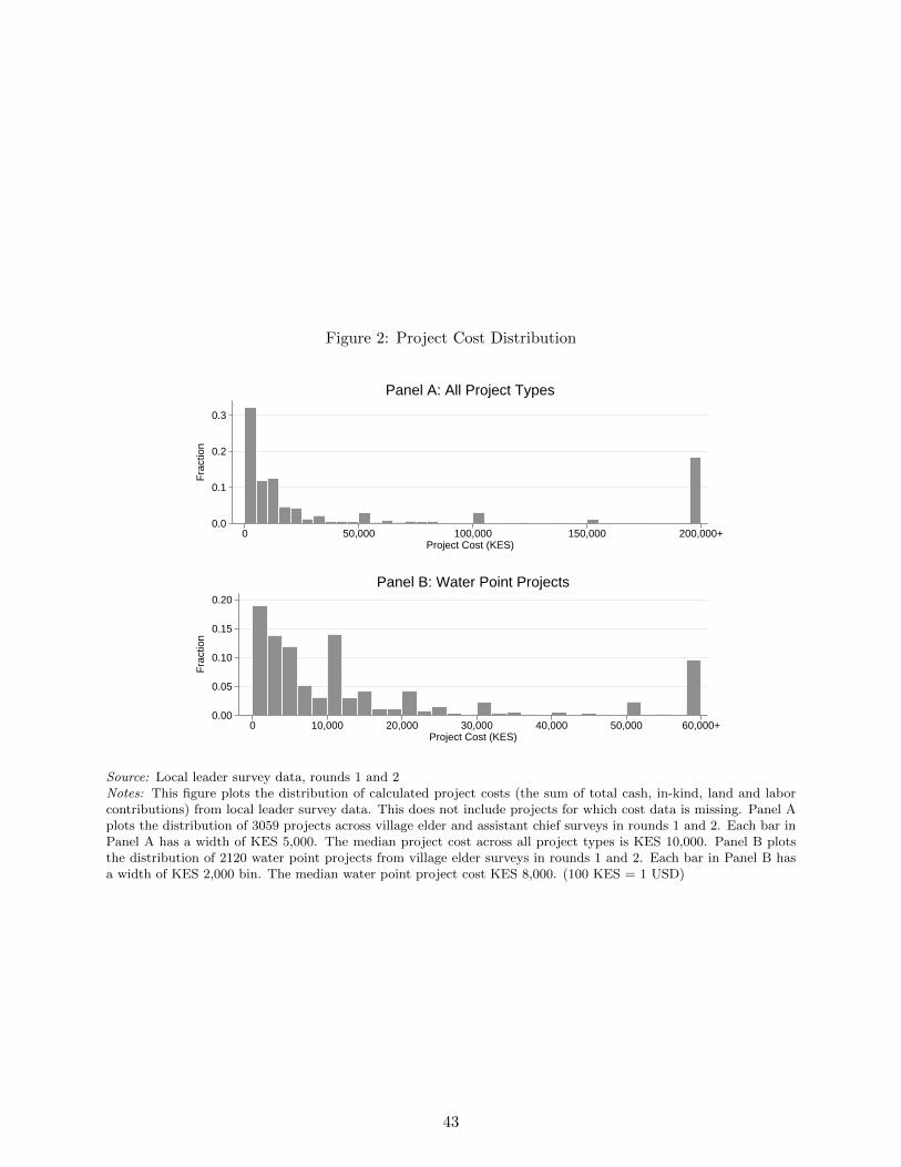
Figure 2: Project Cost Distribution

0.0

0.1

0.2

0.3

Fra

ctio

n

0 50,000 100,000 150,000 200,000+Project Cost (KES)

Panel A: All Project Types

0.00

0.05

0.10

0.15

0.20

Fra

ctio

n

0 10,000 20,000 30,000 40,000 50,000 60,000+Project Cost (KES)

Panel B: Water Point Projects

Source: Local leader survey data, rounds 1 and 2Notes: This figure plots the distribution of calculated project costs (the sum of total cash, in-kind, land and laborcontributions) from local leader survey data. This does not include projects for which cost data is missing. Panel Aplots the distribution of 3059 projects across village elder and assistant chief surveys in rounds 1 and 2. Each bar inPanel A has a width of KES 5,000. The median project cost across all project types is KES 10,000. Panel B plotsthe distribution of 2120 water point projects from village elder surveys in rounds 1 and 2. Each bar in Panel B hasa width of KES 2,000 bin. The median water point project cost KES 8,000. (100 KES = 1 USD)

43

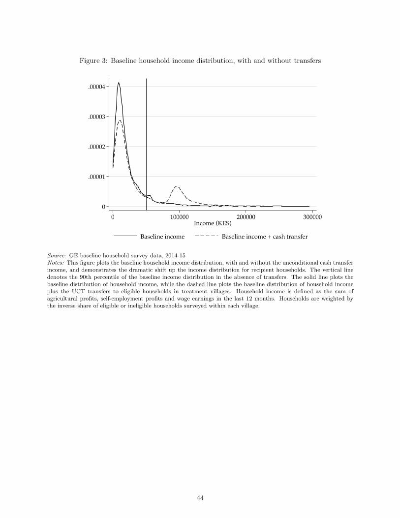
Figure 3: Baseline household income distribution, with and without transfers

0

.00001

.00002

.00003

.00004

0 100000 200000 300000Income (KES)

Baseline income Baseline income + cash transfer

Source: GE baseline household survey data, 2014-15Notes: This figure plots the baseline household income distribution, with and without the unconditional cash transferincome, and demonstrates the dramatic shift up the income distribution for recipient households. The vertical linedenotes the 90th percentile of the baseline income distribution in the absence of transfers. The solid line plots thebaseline distribution of household income, while the dashed line plots the baseline distribution of household incomeplus the UCT transfers to eligible households in treatment villages. Household income is defined as the sum ofagricultural profits, self-employment profits and wage earnings in the last 12 months. Households are weighted bythe inverse share of eligible or ineligible households surveyed within each village.

44

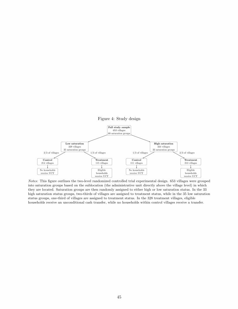
Figure 4: Study design

Full study sample653 villages

68 saturation groups

High saturation324 villages

33 saturation groups

Low saturation329 villages

35 saturation groups

Treatment213 villages

Control111 villages

Treatment115 villages

Control214 villages

Eligiblehouseholds

receive UCT

No householdsreceive UCT

Eligiblehouseholds

receive UCT

No householdsreceive UCT

2/3 of villages1/3 of villages1/3 of villages2/3 of villages

Notes: This figure outlines the two-level randomized controlled trial experimental design. 653 villages were groupedinto saturation groups based on the sublocation (the administrative unit directly above the village level) in whichthey are located. Saturation groups are then randomly assigned to either high or low saturation status. In the 33high saturation status groups, two-thirds of villages are assigned to treatment status, while in the 35 low saturationstatus groups, one-third of villages are assigned to treatment status. In the 328 treatment villages, eligiblehouseholds receive an unconditional cash transfer, while no households within control villages receive a transfer.

45

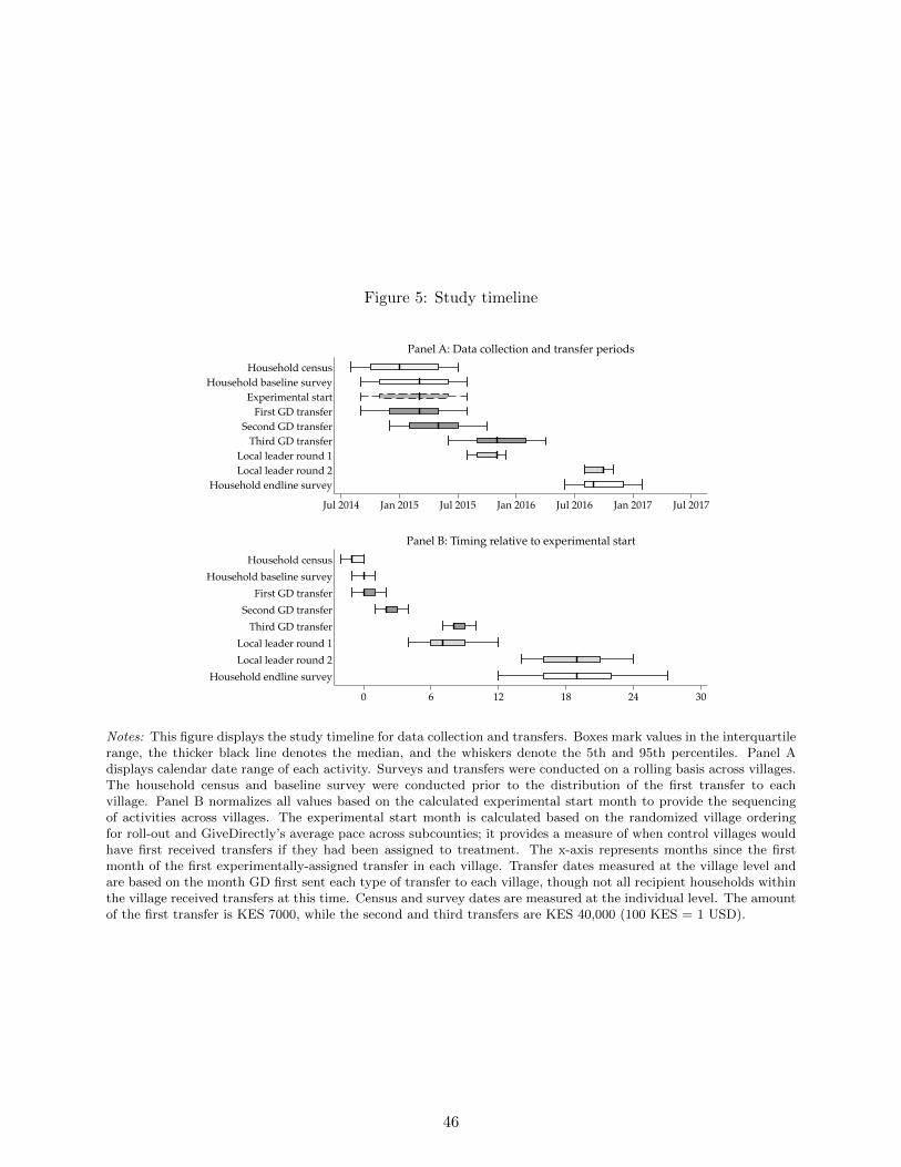
Figure 5: Study timeline

Household censusHousehold baseline survey

Experimental startFirst GD transfer

Second GD transferThird GD transfer

Local leader round 1Local leader round 2

Household endline survey

Jul 2014 Jan 2015 Jul 2015 Jan 2016 Jul 2016 Jan 2017 Jul 2017

Panel A: Data collection and transfer periods

Household censusHousehold baseline survey

First GD transferSecond GD transfer

Third GD transferLocal leader round 1Local leader round 2

Household endline survey

0 6 12 18 24 30

Panel B: Timing relative to experimental start

Notes: This figure displays the study timeline for data collection and transfers. Boxes mark values in the interquartilerange, the thicker black line denotes the median, and the whiskers denote the 5th and 95th percentiles. Panel Adisplays calendar date range of each activity. Surveys and transfers were conducted on a rolling basis across villages.The household census and baseline survey were conducted prior to the distribution of the first transfer to eachvillage. Panel B normalizes all values based on the calculated experimental start month to provide the sequencingof activities across villages. The experimental start month is calculated based on the randomized village orderingfor roll-out and GiveDirectly’s average pace across subcounties; it provides a measure of when control villages wouldhave first received transfers if they had been assigned to treatment. The x-axis represents months since the firstmonth of the first experimentally-assigned transfer in each village. Transfer dates measured at the village level andare based on the month GD first sent each type of transfer to each village, though not all recipient households withinthe village received transfers at this time. Census and survey dates are measured at the individual level. The amountof the first transfer is KES 7000, while the second and third transfers are KES 40,000 (100 KES = 1 USD).

46

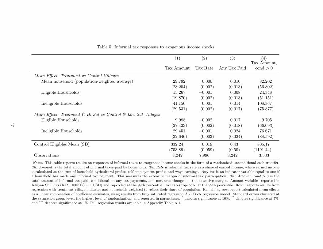
Table 5: Informal tax responses to exogenous income shocks

(1) (2) (3) (4)

Tax Amount Tax Rate Any Tax PaidTax Amount,

cond > 0

Mean Effect, Treatment vs Control VillagesMean household (population-weighted average) 29.792 0.000 0.010 82.202

(23.204) (0.002) (0.013) (56.802)Eligible Housheolds 15.267 −0.001 0.008 24.348

(19.870) (0.002) (0.013) (51.151)Ineligible Households 41.156 0.001 0.014 108.367

(29.531) (0.002) (0.017) (75.877)Mean Effect, Treatment & Hi Sat vs Control & Low Sat Villages

Eligible Households 9.988 −0.002 0.017 −9.705(27.423) (0.002) (0.018) (66.093)

Ineligible Households 29.451 −0.001 0.024 76.671(32.646) (0.003) (0.024) (88.592)

Control Eligibles Mean (SD) 332.24 0.019 0.43 805.17(753.89) (0.059) (0.50) (1191.44)

Observations 8,242 7,996 8,242 3,533

Notes: This table reports results on responses of informal taxes to exogenous income shocks in the form of a randomized unconditional cash transfer.Tax Amount is the total amount of informal taxes paid by households. Tax Rate is informal tax rate as a share of earned income, where earned incomeis calculated as the sum of household agricultural profits, self-employment profits and wage earnings. Any tax is an indicator variable equal to one ifa household has made any informal tax payment. This measures the extensive margin of informal tax participation. Tax Amount, cond > 0 is thetotal amount of informal tax paid, conditional on any tax payments, and measures changes on the extensive margin. Amount variables reported inKenyan Shillings (KES, 100KES = 1 USD) and topcoded at the 99th percentile. Tax rates topcoded at the 99th percentile. Row 1 reports results fromregression with treatment village indicator and households weighted to reflect their share of population. Remaining rows report calculated mean effectsas a linear combination of coefficient estimates, using results from fully saturated regression ANCOVA regression model. Standard errors clustered atthe saturation group level, the highest level of randomization, and reported in parentheses. * denotes significance at 10%, ** denotes significance at 5%,and *** denotes significance at 1%. Full regression results available in Appendix Table A.1.

47

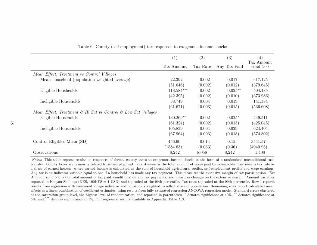
Table 6: County (self-employment) tax responses to exogenous income shocks

(1) (2) (3) (4)

Tax Amount Tax Rate Any Tax PaidTax Amount

cond > 0

Mean Effect, Treatment vs Control VillagesMean household (population-weighted average) 22.392 0.002 0.017 −17.125

(51.646) (0.002) (0.012) (379.645)Eligible Housheolds 118.584∗∗∗ 0.002 0.025∗∗ 504.485

(42.395) (0.002) (0.010) (373.986)Ineligible Households 38.749 0.004 0.019 141.384

(61.671) (0.003) (0.015) (536.608)Mean Effect, Treatment & Hi Sat vs Control & Low Sat Villages

Eligible Households 130.269∗∗ 0.002 0.025∗ 449.511(61.324) (0.002) (0.015) (425.045)

Ineligible Households 105.839 0.004 0.029 624.404(67.964) (0.003) (0.018) (574.802)

Control Eligibles Mean (SD) 456.90 0.014 0.15 3441.57(1584.63) (0.063) (0.36) (4940.95)

Observations 8,242 8,058 8,242 1,408

Notes: This table reports results on responses of formal county taxes to exogenous income shocks in the form of a randomized unconditional cashtransfer. County taxes are primarily related to self-employment. Tax Amount is the total amount of taxes paid by households. Tax Rate is tax rate asa share of earned income, where earned income is calculated as the sum of household agricultural profits, self-employment profits and wage earnings.Any tax is an indicator variable equal to one if a household has made any tax payment. This measures the extensive margin of tax participation. TaxAmount, cond > 0 is the total amount of tax paid, conditional on any tax payments, and measures changes on the extensive margin. Amount variablesreported in Kenyan Shillings (KES, 100KES = 1 USD) and topcoded at the 99th percentile. Tax rates topcoded at the 99th percentile. Row 1 reportsresults from regression with treatment village indicator and households weighted to reflect share of population. Remaining rows report calculated meaneffects as a linear combination of coefficient estimates, using results from fully saturated regression ANCOVA regression model. Standard errors clusteredat the saturation group level, the highest level of randomization, and reported in parentheses. * denotes significance at 10%, ** denotes significance at5%, and *** denotes significance at 1%. Full regression results available in Appendix Table A.3.

48

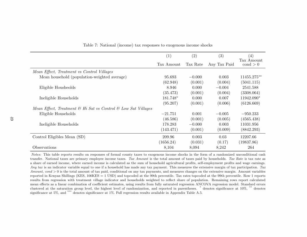
Table 7: National (income) tax responses to exogenous income shocks

(1) (2) (3) (4)

Tax Amount Tax Rate Any Tax PaidTax Amount

cond > 0

Mean Effect, Treatment vs Control VillagesMean household (population-weighted average) 95.693 −0.000 0.003 11455.275∗∗

(62.948) (0.001) (0.004) (5041.115)Eligible Housheolds 8.946 0.000 −0.004 2541.588

(35.473) (0.001) (0.004) (3308.064)Ineligible Households 181.748∗ 0.000 0.007 11942.090∗

(95.207) (0.001) (0.006) (6126.669)Mean Effect, Treatment & Hi Sat vs Control & Low Sat Villages

Eligible Households −21.751 0.001 −0.005 −950.233(46.586) (0.001) (0.005) (4565.438)

Ineligible Households 178.283 −0.000 0.003 11031.956(143.471) (0.001) (0.009) (8842.293)

Control Eligibles Mean (SD) 209.96 0.003 0.03 12207.66(1656.24) (0.031) (0.17) (19837.86)

Observations 8,104 8,094 8,242 264

Notes: This table reports results on responses of formal county taxes to exogenous income shocks in the form of a randomized unconditional cashtransfer. National taxes are primary employee income taxes. Tax Amount is the total amount of taxes paid by households. Tax Rate is tax rate asa share of earned income, where earned income is calculated as the sum of household agricultural profits, self-employment profits and wage earnings.Any tax is an indicator variable equal to one if a household has made any tax payment. This measures the extensive margin of tax participation. TaxAmount, cond > 0 is the total amount of tax paid, conditional on any tax payments, and measures changes on the extensive margin. Amount variablesreported in Kenyan Shillings (KES, 100KES = 1 USD) and topcoded at the 99th percentile. Tax rates topcoded at the 99th percentile. Row 1 reportsresults from regression with treatment village indicator and households weighted to reflect share of population. Remaining rows report calculatedmean effects as a linear combination of coefficient estimates, using results from fully saturated regression ANCOVA regression model. Standard errorsclustered at the saturation group level, the highest level of randomization, and reported in parentheses. * denotes significance at 10%, ** denotessignificance at 5%, and *** denotes significance at 1%. Full regression results available in Appendix Table A.5.

49

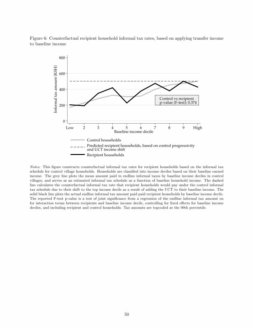
Figure 6: Counterfactual recipient household informal tax rates, based on applying transfer incometo baseline income

Control vs recipientp-value (F-test): 0.374

0

200

400

600

800In

form

al ta

x am

ount

(KSH

)

Low 2 3 4 5 6 7 8 9 HighBaseline income decile

Control householdsPredicted recipient households, based on control progressivityand UCT income shiftRecipient households

Notes: This figure constructs counterfactual informal tax rates for recipient households based on the informal taxschedule for control village households. Households are classified into income deciles based on their baseline earnedincome. The grey line plots the mean amount paid in endline informal taxes by baseline income deciles in controlvillages, and serves as an estimated informal tax schedule as a function of baseline household income. The dashedline calculates the counterfactual informal tax rate that recipient households would pay under the control informaltax schedule due to their shift to the top income decile as a result of adding the UCT to their baseline income. Thesolid black line plots the actual endline informal tax amount paid paid recipient households by baseline income decile.The reported F-test p-value is a test of joint significance from a regression of the endline informal tax amount onfor interaction terms between recipients and baseline income decile, controlling for fixed effects for baseline incomedeciles, and including recipient and control households. Tax amounts are topcoded at the 99th percentile.

50

Table 8: Comparing endline informal taxes paid by recipient households by income deciles

(1) (2) (3)

Baseline Income DecileEndline Income Decile,

w/o UCT transferEndline Income decile,

w/ UCT transfer

Income Decile 1 × Recipient 30.04 −71.40 −74.21(48.68) (47.29) (59.42)

Income Decile 2 × Recipient −33.24 72.26 74.32(39.41) (49.65) (87.11)

Income Decile 3 × Recipient 66.68 −58.90 −125.3∗∗

(63.63) (49.52) (50.38)

Income Decile 4 × Recipient 94.73 114.9 −55.91(73.35) (77.22) (81.31)

Income Decile 5 × Recipient −78.95 −99.36 −174.9∗∗

(52.24) (60.59) (67.88)

Income Decile 6 × Recipient 60.62 −44.91 −165.6∗∗

(57.22) (64.64) (70.35)

Income Decile 7 × Recipient 71.07 39.55 −110.4∗∗

(77.66) (70.34) (55.26)

Income Decile 8 × Recipient −77.03 106.1∗ 23.42(75.23) (63.68) (54.45)

Income Decile 9 × Recipient 26.60 −36.13 27.24(83.45) (63.06) (56.31)

Income Decile 10 × Recipient −70.83 −81.72 −53.29(75.86) (71.35) (63.79)

Income Decile FEs Y es Y es Y es

Observations 5,988 5,988 5,988Mean Informal Tax Amount 344 344 344Joint test of significance (p-value) 0.374 0.068 0.005Adjusted R2 0.180 0.177 0.177

Notes: Dependent variable: endline household informal tax amount. The sample for these regressions include all control householdsand recipient households. Each column reports regression coefficients on interaction terms between an indicator for the income decile,based on the measure of income deciles indicated in the column heading, and recipient households. Each regression also includesindicators for income deciles for control households, so that the coefficients reported in the table capture the additional effect forrecipient households by income decile. Standard errors clustered at the village level and reported in parentheses. * denotes significanceat 10%, ** denotes significance at 5%, and *** denotes significance at 1%. Dependent variable topcoded at the 99th percentile. Endlineincome deciles calculated on the basis of control households only. Household income defined as the sum of agricultural profits, self-employment profits and after-tax wage earnings. UCT income distributed over the last 12 months included for eligible households intreatment villages, assuming that households received transfers in experimental start month. This is a conservative assumption andmay underestimate the actual amount recipient households may have received in the past 12 months if they did not begin receivingtransfers right away.

51

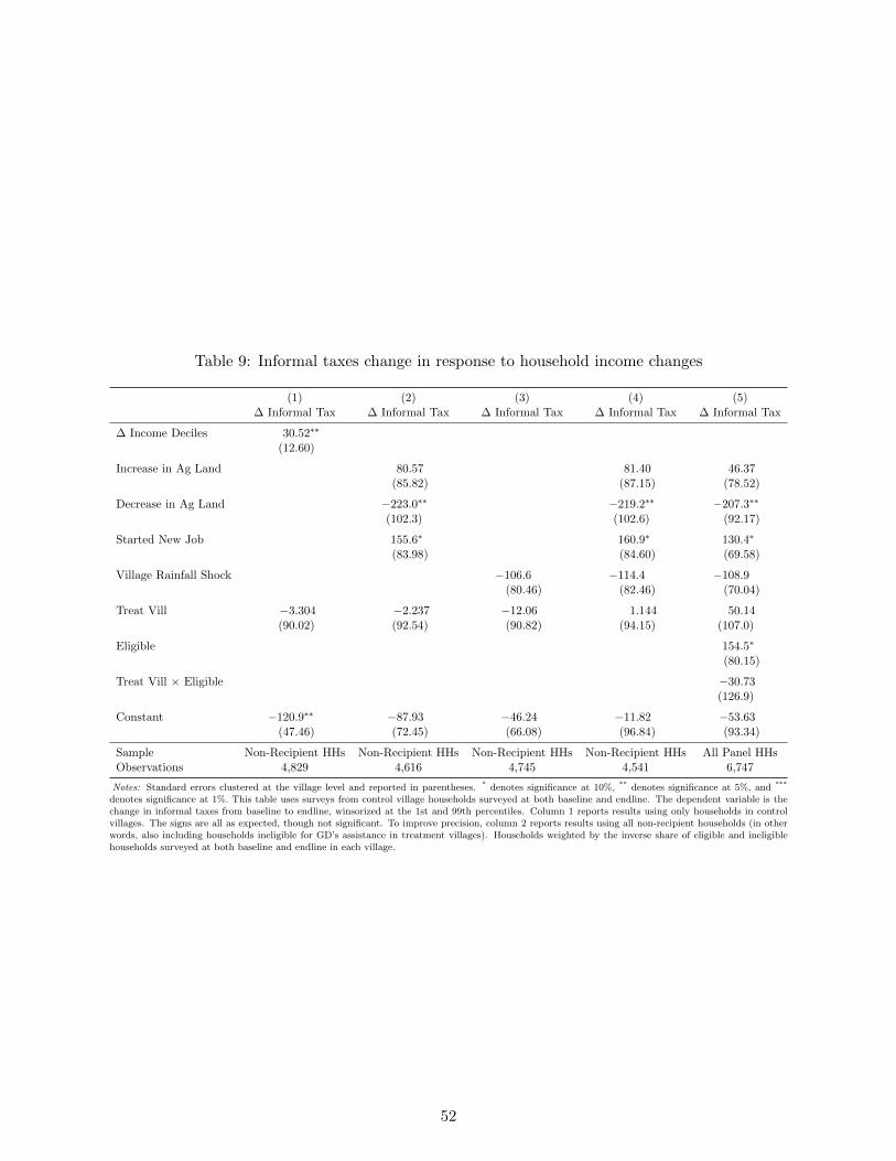
Table 9: Informal taxes change in response to household income changes

(1) (2) (3) (4) (5)∆ Informal Tax ∆ Informal Tax ∆ Informal Tax ∆ Informal Tax ∆ Informal Tax

∆ Income Deciles 30.52∗∗

(12.60)

Increase in Ag Land 80.57 81.40 46.37(85.82) (87.15) (78.52)

Decrease in Ag Land −223.0∗∗ −219.2∗∗ −207.3∗∗

(102.3) (102.6) (92.17)

Started New Job 155.6∗ 160.9∗ 130.4∗

(83.98) (84.60) (69.58)

Village Rainfall Shock −106.6 −114.4 −108.9(80.46) (82.46) (70.04)

Treat Vill −3.304 −2.237 −12.06 1.144 50.14(90.02) (92.54) (90.82) (94.15) (107.0)

Eligible 154.5∗

(80.15)

Treat Vill × Eligible −30.73(126.9)

Constant −120.9∗∗ −87.93 −46.24 −11.82 −53.63(47.46) (72.45) (66.08) (96.84) (93.34)

Sample Non-Recipient HHs Non-Recipient HHs Non-Recipient HHs Non-Recipient HHs All Panel HHsObservations 4,829 4,616 4,745 4,541 6,747

Notes: Standard errors clustered at the village level and reported in parentheses. * denotes significance at 10%, ** denotes significance at 5%, and ***

denotes significance at 1%. This table uses surveys from control village households surveyed at both baseline and endline. The dependent variable is thechange in informal taxes from baseline to endline, winsorized at the 1st and 99th percentiles. Column 1 reports results using only households in controlvillages. The signs are all as expected, though not significant. To improve precision, column 2 reports results using all non-recipient households (in otherwords, also including households ineligible for GD’s assistance in treatment villages). Households weighted by the inverse share of eligible and ineligiblehouseholds surveyed at both baseline and endline in each village.

52

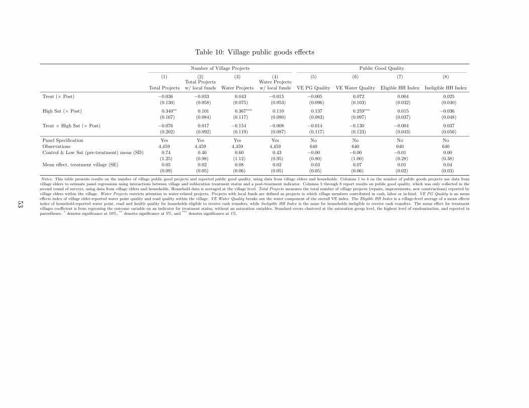
Table 10: Village public goods effects

Number of Village Projects Public Good Quality

(1) (2) (3) (4) (5) (6) (7) (8)

Total ProjectsTotal Projectsw/ local funds Water Projects

Water Projectsw/ local funds VE PG Quality VE Water Quality Eligible HH Index Ineligible HH Index

Treat (× Post) −0.036 −0.033 0.043 −0.015 −0.005 0.072 0.004 0.025(0.130) (0.058) (0.075) (0.053) (0.096) (0.103) (0.032) (0.040)

High Sat (× Post) 0.340∗∗ 0.101 0.367∗∗∗ 0.110 0.137 0.259∗∗∗ 0.015 −0.036(0.167) (0.084) (0.117) (0.080) (0.083) (0.097) (0.037) (0.048)

Treat × High Sat (× Post) −0.076 0.017 −0.154 −0.008 −0.014 −0.130 −0.004 0.037(0.202) (0.092) (0.119) (0.087) (0.117) (0.123) (0.043) (0.056)

Panel Specification Yes Yes Yes Yes No No No NoObservations 4,459 4,459 4,459 4,459 640 640 640 640Control & Low Sat (pre-treatment) mean (SD) 0.74 0.46 0.60 0.43 −0.00 −0.00 −0.01 0.00

(1.25) (0.98) (1.12) (0.95) (0.80) (1.00) (0.28) (0.38)Mean effect, treatment village (SE) 0.05 0.02 0.08 0.02 0.03 0.07 0.01 0.04

(0.09) (0.05) (0.06) (0.05) (0.05) (0.06) (0.02) (0.03)

Notes: This table presents results on the number of village public good projects and reported public good quality, using data from village elders and households. Columns 1 to 4 on the number of public goods projects use data fromvillage elders to estimate panel regressions using interactions between village and sublocation treatment status and a post-treatment indicator. Columns 5 through 8 report results on public good quality, which was only collected in thesecond round of surveys, using data from village elders and households. Household data is averaged at the village level. Total Projects measures the total number of village projects (repairs, improvements, new constructions) reported byvillage elders within the village. Water Projects restricts attention to water-related projects. Projects with local funds are defined as projects in which village members contributed in cash, labor or in-kind. VE PG Quality is an meaneffects index of village elder-reported water point quality and road quality within the village. VE Water Quality breaks out the water component of the overall VE index. The Eligible HH Index is a village-level average of a mean effectsindex of household-reported water point, road and health quality for households eligible to receive cash transfers, while Ineligible HH Index is the same for households ineligible to receive cash transfers. The mean effect for treatmentvillages coefficient is from regressing the outcome variable on an indicator for treatment status, without an saturation variables. Standard errors clustered at the saturation group level, the highest level of randomization, and reported inparentheses. * denotes significance at 10%, ** denotes significance at 5%, and *** denotes significance at 1%.

53

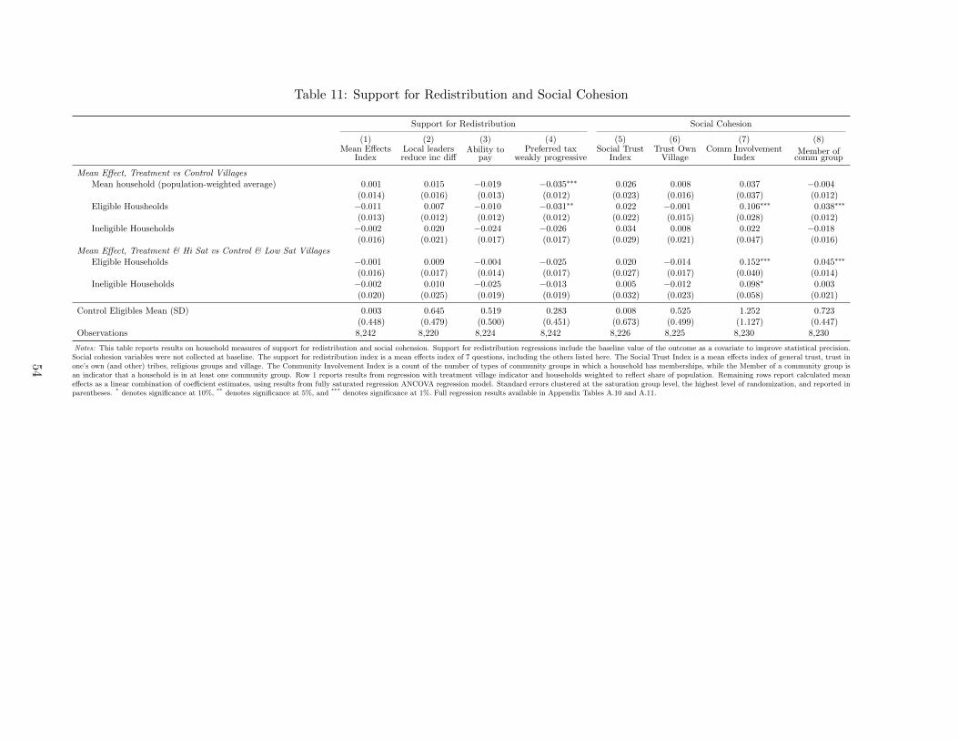
Table 11: Support for Redistribution and Social Cohesion

Support for Redistribution Social Cohesion

(1) (2) (3) (4) (5) (6) (7) (8)Mean Effects

IndexLocal leadersreduce inc diff

Ability topay

Preferred taxweakly progressive

Social TrustIndex

Trust OwnVillage

Comm InvolvementIndex

Member ofcomm group

Mean Effect, Treatment vs Control VillagesMean household (population-weighted average) 0.001 0.015 −0.019 −0.035∗∗∗ 0.026 0.008 0.037 −0.004

(0.014) (0.016) (0.013) (0.012) (0.023) (0.016) (0.037) (0.012)Eligible Housheolds −0.011 0.007 −0.010 −0.031∗∗ 0.022 −0.001 0.106∗∗∗ 0.038∗∗∗

(0.013) (0.012) (0.012) (0.012) (0.022) (0.015) (0.028) (0.012)Ineligible Households −0.002 0.020 −0.024 −0.026 0.034 0.008 0.022 −0.018

(0.016) (0.021) (0.017) (0.017) (0.029) (0.021) (0.047) (0.016)Mean Effect, Treatment & Hi Sat vs Control & Low Sat Villages

Eligible Households −0.001 0.009 −0.004 −0.025 0.020 −0.014 0.152∗∗∗ 0.045∗∗∗

(0.016) (0.017) (0.014) (0.017) (0.027) (0.017) (0.040) (0.014)Ineligible Households −0.002 0.010 −0.025 −0.013 0.005 −0.012 0.098∗ 0.003

(0.020) (0.025) (0.019) (0.019) (0.032) (0.023) (0.058) (0.021)

Control Eligibles Mean (SD) 0.003 0.645 0.519 0.283 0.008 0.525 1.252 0.723(0.448) (0.479) (0.500) (0.451) (0.673) (0.499) (1.127) (0.447)

Observations 8,242 8,220 8,224 8,242 8,226 8,225 8,230 8,230

Notes: This table reports results on household measures of support for redistribution and social cohension. Support for redistribution regressions include the baseline value of the outcome as a covariate to improve statistical precision.Social cohesion variables were not collected at baseline. The support for redistribution index is a mean effects index of 7 questions, including the others listed here. The Social Trust Index is a mean effects index of general trust, trust inone’s own (and other) tribes, religious groups and village. The Community Involvement Index is a count of the number of types of community groups in which a household has memberships, while the Member of a community group isan indicator that a household is in at least one community group. Row 1 reports results from regression with treatment village indicator and households weighted to reflect share of population. Remaining rows report calculated meaneffects as a linear combination of coefficient estimates, using results from fully saturated regression ANCOVA regression model. Standard errors clustered at the saturation group level, the highest level of randomization, and reported inparentheses. * denotes significance at 10%, ** denotes significance at 5%, and *** denotes significance at 1%. Full regression results available in Appendix Tables A.10 and A.11.

54

A Appendix

Figure A.1: Informal taxes over the household wealth distribution

0

.001

.002

.003

Den

sity

0 500 1,000 1,500 2,000Total Wealth (KES '000s)

Panel A: Wealth Distribution

0.33

0.55Mean: 0.43

SD: 0.01

0

.2

.4

.6

.8

Low 2 3 4 5 6 7 8 9 High

Panel B: Any informal tax contribution

222

847Mean: 388

SD: 11

200

400

600

800

1000

Low 2 3 4 5 6 7 8 9 HighWealth Decile

Panel C: Informal tax amount (KES)

0.006

0.001

Mean: 0.003SD: 0.000

0

.002

.004

.006

.008

Low 2 3 4 5 6 7 8 9 HighWealth Decile

Panel D: Informal taxes as share of wealth

Source: GE Household Baseline Survey (2014-15)Notes: This figure plots baseline informal tax data against baseline household wealth data. Panel A plots thehousehold wealth distribution. Household wealth is defined as the sum of household durable assets, livestock, homevalue and land value. Gray vertical lines denote the wealth deciles that correspond with Panels B to D. The rangefrom 9th to 1st decile is KES 667,200. In Panels B through D, markers denote the mean and bars plot the 95percent confidence intervals and labels report the values of for the 1st and 10th decile. Panel B displays the share ofhouseholds making any informal tax contributions by wealth decile. The positive gradient indicates a greater share ofwealthier households participating in informal taxes. Panel C displays the mean amount of informal tax contributionsby decile. Values are reported in Kenyan Shillings (1 USD = 100 KES) and are topcoded at the 99th percentile.Panel D displays informal taxes as a percent of household wealth and are also topcoded at the 99th percentile. Whilericher households pay more informal tax, they pay less as a share of their wealth.

55

Table A.1: Informal tax responses to exogenous income shocks

(1) (2) (3) (4) (5) (6) (7) (8)

Tax Amount Tax Amount Tax Rate Tax Rate Any Tax Paid Any Tax PaidTax Amount,

cond > 0Tax Amount,

cond > 0

Treat Village (β1) 29.792 101.943∗∗ 0.000 0.009∗∗ 0.010 0.007 82.202 253.499∗∗

(23.204) (44.258) (0.002) (0.004) (0.013) (0.022) (56.802) (116.236)

Eligible Household (β2) 3.037 0.000 0.037∗∗ −75.133(24.261) (0.002) (0.018) (66.083)

Treat Village × Eligible (β3) −97.548∗∗ −0.009∗ −0.014 −215.357(44.395) (0.005) (0.025) (133.597)

High Sat Sublocation (β4) 37.378 0.004 0.013 81.741(42.851) (0.003) (0.026) (107.003)

Treat Village × High Sat (β5) −109.870 −0.013∗∗ 0.004 −258.568(66.497) (0.005) (0.033) (168.564)

Eligible × High Sat (β6) −58.807 −0.006 −0.010 −136.053(51.219) (0.004) (0.032) (129.311)

Treat Village × Eligible × High Sat (β7) 136.892∗ 0.013∗∗ 0.017 265.034(75.710) (0.006) (0.042) (198.084)

Weights Yes No Yes No Yes No Yes NoObservations 8,242 8,242 7,996 7,996 8,242 8,242 3,533 3,533Control Eligibles Mean (SD) 332.24 332.24 0.019 0.019 0.43 0.43 805.17 805.17

(753.89) (753.89) (0.059) (0.059) (0.50) (0.50) (1191.44) (1191.44)

Mean Effect, Treatment vs Control VillagesEligible Households 15.267 −0.001 0.008 24.348

(19.870) (0.002) (0.013) (51.151)Ineligible Households 41.156 0.001 0.014 108.367

(29.531) (0.002) (0.017) (75.877)Mean Effect, Treatment & Hi Sat vs Control & Low Sat Villages

Eligible Households 9.988 −0.002 0.017 −9.705(27.423) (0.002) (0.018) (66.093)

Ineligible Households 29.451 −0.001 0.024 76.671(32.646) (0.003) (0.024) (88.592)

Joint F-Test for spillover terms (p-value) 0.452 0.126 0.809 0.571

Notes: This table reports results on responses of informal taxes to exogenous income shocks in the form of a randomized unconditional cash transfer. Each column reports results from a separate ANCOVA regression, includingthe baseline value of the outcome variable to improve statistical power. Tax Amount is the total amount of informal taxes paid by households, including labor and in-kind contributions. Labor contributions are evaluated atthe median agricultural wage in control villages, as reported in village elder surveys. Tax Rate is informal tax rate as a share of earned income, where earned income is calculated as the sum of household agricultural profits,self-employment profits and wage earnings. Any tax is an indicator variable equal to one if a household has made any informal tax payment in cash, labor or in-kind. This measures the extensive margin of informal taxparticipation. Tax Amount, cond > 0 is the total amount of informal tax paid, conditional on any informal tax payments, and measures changes on the extensive margin. Amount variables reported in Kenyan Shillings (KES,100KES = 1 USD) and topcoded at the 99th percentile. Tax rates topcoded at the 99th percentile. The mean effects calculated in the bottom panel are linear combinations of the regression coefficients. When comparingthe mean effect between treatment versus control villages, I take the share of households in high versus low saturation sublocations into account. The mean effect for eligible households for treatment versus control villagesis (β1 + β3 + (1/3)β4 + (2/3)β5 + (1/3)β6 + (2/3)β7), while the mean effect for ineligible households is (β1 + β3 + β4). I then compare eligible and ineligible households in treatment villages in high-saturation areas withcontrol villages in low-saturation areas: for eligible households and (β1 + β3 + β4 + β5 + β6 + β7) for ineligible households. When indicated, regression weights are based on the inverse share of households surveyed within avillage by eligibility status. Standard errors clustered at the saturation group level, the highest level of randomization, and reported in parentheses. * denotes significance at 10%, ** denotes significance at 5%, and *** denotessignificance at 1%.

56

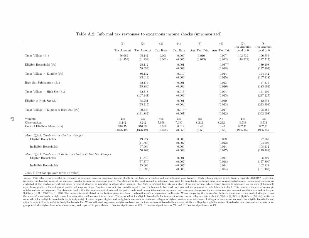
Table A.2: Informal tax responses to exogenous income shocks (unwinsorized)

(1) (2) (3) (4) (5) (6) (7) (8)

Tax Amount Tax Amount Tax Rate Tax Rate Any Tax Paid Any Tax PaidTax Amount,

cond > 0Tax Amount,

cond > 0

Treat Village (β1) 56.089 95.147 0.001 0.009∗ 0.010 0.007 102.739 196.756(34.459) (61.259) (0.002) (0.005) (0.013) (0.022) (78.521) (147.717)

Eligible Household (β2) −25.112 −0.001 0.037∗∗ −139.498(59.059) (0.003) (0.018) (137.403)

Treat Village × Eligible (β3) −86.132 −0.010∗ −0.014 −164.042(83.613) (0.006) (0.025) (197.418)

High Sat Sublocation (β4) 42.175 −0.001 0.013 77.379(78.880) (0.004) (0.026) (183.064)

Treat Village × High Sat (β5) −62.318 −0.013∗∗ 0.004 −171.207(107.441) (0.006) (0.033) (247.227)

Eligible × High Sat (β6) −68.251 −0.001 −0.010 −142.651(95.315) (0.004) (0.032) (223.191)

Treat Village × Eligible × High Sat (β7) 90.749 0.015∗∗ 0.017 195.367(131.882) (0.007) (0.042) (302.098)

Weights Yes No Yes No Yes No Yes NoObservations 8,242 8,242 7,956 7,956 8,242 8,242 3,533 3,533Control Eligibles Mean (SD) 376.35 376.35 0.018 0.018 0.43 0.43 867.31 867.31

(1326.42) (1326.42) (0.058) (0.058) (0.50) (0.50) (1905.35) (1905.35)

Mean Effect, Treatment vs Control VillagesEligible Households 19.277 −0.000 0.008 27.065

(41.880) (0.002) (0.013) (94.906)Ineligible Households 67.660 0.000 0.014 108.412

(50.462) (0.003) (0.017) (119.489)Mean Effect, Treatment & Hi Sat vs Control & Low Sat Villages

Eligible Households 11.370 −0.001 0.017 −8.397(57.370) (0.002) (0.018) (127.800)

Ineligible Households 75.004 −0.005∗ 0.024 102.929(61.896) (0.003) (0.024) (151.400)

Joint F-Test for spillover terms (p-value)

Notes: This table reports results on responses of informal taxes to exogenous income shocks in the form of a randomized unconditional cash transfer. Each column reports results from a separate ANCOVA regression,including the baseline value of the outcome variable to improve statistical power. Tax Amount is the total amount of informal taxes paid by households, including labor and in-kind contributions. Labor contributions areevaluated at the median agricultural wage in control villages, as reported in village elder surveys. Tax Rate is informal tax rate as a share of earned income, where earned income is calculated as the sum of householdagricultural profits, self-employment profits and wage earnings. Any tax is an indicator variable equal to one if a household has made any informal tax payment in cash, labor or in-kind. This measures the extensive marginof informal tax participation. Tax Amount, cond > 0 is the total amount of informal tax paid, conditional on any informal tax payments, and measures changes on the extensive margin. Amount variables reported in KenyanShillings (KES, 100KES = 1 USD). The mean effects calculated in the bottom panel are linear combinations of the regression coefficients. When comparing the mean effect between treatment versus control villages, I takethe share of households in high versus low saturation sublocations into account. The mean effect for eligible households for treatment versus control villages is (β1 + β3 + (1/3)β4 + (2/3)β5 + (1/3)β6 + (2/3)β7), while themean effect for ineligible households is (β1 + β3 + β4). I then compare eligible and ineligible households in treatment villages in high-saturation areas with control villages in low-saturation areas: for eligible households and(β1 +β3 +β4 +β5 +β6 +β7) for ineligible households. When indicated, regression weights are based on the inverse share of households surveyed within a village by eligibility status. Standard errors clustered at the saturationgroup level, the highest level of randomization, and reported in parentheses. * denotes significance at 10%, ** denotes significance at 5%, and *** denotes significance at 1%.

57

Table A.3: County (self-employment) tax responses to exogenous income shocks

(1) (2) (3) (4) (5) (6) (7) (8)

Tax Amount Tax Amount Tax Rate Tax Rate Any Tax Paid Any Tax PaidTax Amount

cond > 0Tax Amount

cond > 0

Treat Village (β1) 22.392 184.900∗ 0.002 0.006 0.017 0.025 −17.125 996.685(51.646) (109.637) (0.002) (0.005) (0.012) (0.026) (379.645) (839.710)

Eligible Household (β2) −32.036 −0.000 −0.010 −182.537(52.928) (0.002) (0.014) (479.096)

Treat Village × Eligible (β3) 39.460 −0.002 0.016 168.071(106.035) (0.005) (0.024) (1038.226)

High Sat Sublocation (β4) 280.331∗∗∗ 0.001 0.027 1821.340∗∗

(89.668) (0.003) (0.019) (729.814)

Treat Village × High Sat (β5) −359.392∗∗ −0.003 −0.023 −2193.621∗

(143.614) (0.006) (0.032) (1187.194)

Eligible × High Sat (β6) −151.186 0.001 −0.009 −1271.017(114.461) (0.004) (0.024) (935.074)

Treat Village × Eligible × High Sat (β7) 136.155 −0.001 −0.012 928.054(159.419) (0.007) (0.033) (1450.175)

Weights Yes No Yes No Yes No Yes NoObservations 8,242 8,242 8,058 8,058 8,242 8,242 1,408 1,408Control Eligibles Mean (SD) 456.90 456.90 0.014 0.014 0.15 0.15 3441.57 3441.57

(1584.63) (1584.63) (0.063) (0.063) (0.36) (0.36) (4940.95) (4940.95)

Mean Effect, Treatment vs Control VillagesEligible Housheolds 118.584∗∗∗ 0.002 0.025∗∗ 504.485

(42.395) (0.002) (0.010) (373.986)Ineligible Households 38.749 0.004 0.019 141.384

(61.671) (0.003) (0.015) (536.608)Mean Effect, Treatment & Hi Sat vs Control & Low Sat Villages

Eligible Households 130.269∗∗ 0.002 0.025∗ 449.511(61.324) (0.002) (0.015) (425.045)

Ineligible Households 105.839 0.004 0.029 624.404(67.964) (0.003) (0.018) (574.802)

Notes: This table reports results on responses of formal county taxes to exogenous income shocks in the form of a randomized unconditional cash transfer. County taxes are primarily related to self-employment. Eachcolumn reports results from a separate ANCOVA regression, including the baseline value of the outcome variable to improve statistical power. Tax Amount is the total amount of taxes paid by households. Tax Rate istax rate as a share of earned income, where earned income is calculated as the sum of household agricultural profits, self-employment profits and wage earnings. Any tax is an indicator variable equal to one if a householdhas made any tax payment. This measures the extensive margin of tax participation. Tax Amount, cond > 0 is the total amount of tax paid, conditional on any tax payments, and measures changes on the extensivemargin. Amount variables reported in Kenyan Shillings (KES, 100KES = 1 USD) and topcoded at the 99th percentile. Tax rates topcoded at the 99th percentile. The mean effects calculated in the bottom panel are linearcombinations of the regression coefficients. When comparing the mean effect between treatment versus control villages, I take the share of households in high versus low saturation sublocations into account. The meaneffect for eligible households for treatment versus control villages is (β1 + β3 + (1/3)β4 + (2/3)β5 + (1/3)β6 + (2/3)β7), while the mean effect for ineligible households is (β1 + β3 + β4). I then compare eligible and ineligiblehouseholds in treatment villages in high-saturation areas with control villages in low-saturation areas: for eligible households and (β1 + β3 + β4 + β5 + β6 + β7) for ineligible households. When indicated, regression weightsare based on the inverse share of households surveyed within a village by eligibility status. Standard errors clustered at the saturation group level, the highest level of randomization, and reported in parentheses. * denotessignificance at 10%, ** denotes significance at 5%, and *** denotes significance at 1%.

58

Table A.4: County (self-employment) tax responses to exogenous income shocks (unwinsorized)

(1) (2) (3) (4) (5) (6) (7) (8)

Tax Amount Tax Amount Tax Rate Tax Rate Any Tax Paid Any Tax PaidTax Amount

cond > 0Tax Amount

cond > 0

Treat Village (β1) 125.553 329.426 0.002 0.006 0.017 0.025 283.024 1446.233(101.225) (205.272) (0.002) (0.005) (0.012) (0.026) (464.633) (1079.888)

Eligible Household (β2) −17.983 −0.000 −0.010 88.772(87.953) (0.002) (0.014) (591.400)

Treat Village × Eligible (β3) 62.222 −0.002 0.016 −69.269(218.538) (0.005) (0.024) (1371.083)

High Sat Sublocation (β4) 485.555∗∗∗ 0.001 0.027 2141.783∗∗

(176.266) (0.003) (0.019) (914.403)

Treat Village × High Sat (β5) −481.852 −0.003 −0.023 −2508.751(304.658) (0.006) (0.032) (1556.618)

Eligible × High Sat (β6) −357.019∗ 0.001 −0.009 −1771.057(213.236) (0.004) (0.024) (1183.241)

Treat Village × Eligible × High Sat (β7) 126.282 −0.001 −0.012 1117.108(338.209) (0.007) (0.033) (1931.094)

Weights Yes No Yes No Yes No Yes NoObservations 8,242 8,242 8,058 8,058 8,242 8,242 1,408 1,408Control Eligibles Mean (SD) 546.48 546.48 0.014 0.014 0.15 0.15 3608.36 3608.36

(2883.33) (2883.33) (0.063) (0.063) (0.36) (0.36) (6628.20) (6628.20)

Mean Effect, Treatment vs Control VillagesEligible Housheolds 197.448∗∗ 0.002 0.025∗∗ 572.777

(87.573) (0.002) (0.010) (527.864)Ineligible Households 170.044 0.004 0.019 487.660

(140.900) (0.003) (0.015) (692.478)Mean Effect, Treatment & Hi Sat vs Control & Low Sat Villages

Eligible Households 164.615 0.002 0.025∗ 356.046(113.539) (0.002) (0.015) (596.589)

Ineligible Households 333.130∗∗ 0.004 0.029 1079.265(166.520) (0.003) (0.018) (731.752)

Notes: This table reports results on responses of formal county taxes to exogenous income shocks in the form of a randomized unconditional cash transfer. County taxes are primarily related to self-employment. Eachcolumn reports results from a separate ANCOVA regression, including the baseline value of the outcome variable to improve statistical power. Tax Amount is the total amount of taxes paid by households. Tax Rateis tax rate as a share of earned income, where earned income is calculated as the sum of household agricultural profits, self-employment profits and wage earnings. Any tax is an indicator variable equal to one if ahousehold has made any tax payment. This measures the extensive margin of tax participation. Tax Amount, cond > 0 is the total amount of tax paid, conditional on any tax payments, and measures changes on theextensive margin. Amount variables reported in Kenyan Shillings (KES, 100KES = 1 USD). The mean effects calculated in the bottom panel are linear combinations of the regression coefficients. When comparing themean effect between treatment versus control villages, I take the share of households in high versus low saturation sublocations into account. The mean effect for eligible households for treatment versus control villages is(β1 + β3 + (1/3)β4 + (2/3)β5 + (1/3)β6 + (2/3)β7), while the mean effect for ineligible households is (β1 + β3 + β4). I then compare eligible and ineligible households in treatment villages in high-saturation areas withcontrol villages in low-saturation areas: for eligible households and (β1 + β3 + β4 + β5 + β6 + β7) for ineligible households. When indicated, regression weights are based on the inverse share of households surveyed withina village by eligibility status. Standard errors clustered at the saturation group level, the highest level of randomization, and reported in parentheses. * denotes significance at 10%, ** denotes significance at 5%, and ***

denotes significance at 1%.

59

Table A.5: National (income) tax responses to exogenous income shocks

(1) (2) (3) (4) (5) (6) (7) (8)

Tax Amount Tax Amount Tax Rate Tax Rate Any Tax Paid Any Tax PaidTax Amount

cond > 0Tax Amount

cond > 0

Treat Village (β1) 95.693 226.775∗ −0.000 0.001 0.003 0.009 11455.275∗∗ 13455.276(62.948) (126.406) (0.001) (0.001) (0.004) (0.008) (5041.115) (8930.295)

Eligible Household (β2) −181.908∗ −0.001 −0.004 −9117.303(92.944) (0.001) (0.007) (5901.083)

Treat Village × Eligible (β3) −136.053 0.001 −0.009 −8356.943(135.739) (0.002) (0.010) (11812.998)

High Sat Sublocation (β4) 38.097 −0.000 −0.004 −307.083(148.093) (0.001) (0.010) (7863.399)

Treat Village × High Sat (β5) −86.589 −0.001 −0.002 −2116.238(185.869) (0.002) (0.012) (12017.328)

Eligible × High Sat (β6) −17.715 0.003 0.006 −4119.813(168.031) (0.002) (0.013) (8706.101)

Treat Village × Eligible × High Sat (β7) −46.267 −0.003 −0.006 494.566(206.693) (0.002) (0.015) (14738.062)

Weights Yes No Yes No Yes No Yes NoObservations 8,104 8,104 8,094 8,094 8,242 8,242 264 264Control Eligibles Mean (SD) 209.96 209.96 0.003 0.003 0.03 0.03 12207.66 12207.66

(1656.24) (1656.24) (0.031) (0.031) (0.17) (0.17) (19837.86) (19837.86)

Mean Effect, Treatment vs Control VillagesEligible Housheolds 8.946 0.000 −0.004 2541.588

(35.473) (0.001) (0.004) (3308.064)Ineligible Households 181.748∗ 0.000 0.007 11942.090∗

(95.207) (0.001) (0.006) (6126.669)Mean Effect, Treatment & Hi Sat vs Control & Low Sat Villages

Eligible Households −21.751 0.001 −0.005 −950.233(46.586) (0.001) (0.005) (4565.438)

Ineligible Households 178.283 −0.000 0.003 11031.956(143.471) (0.001) (0.009) (8842.293)

Notes: This table reports results on responses of formal county taxes to exogenous income shocks in the form of a randomized unconditional cash transfer. National taxes are primary employee income taxes. Each columnreports results from a separate ANCOVA regression, including the baseline value of the outcome variable to improve statistical power. Tax Amount is the total amount of taxes paid by households. Tax Rate is tax rate asa share of earned income, where earned income is calculated as the sum of household agricultural profits, self-employment profits and wage earnings. Any tax is an indicator variable equal to one if a household has madeany tax payment. This measures the extensive margin of tax participation. Tax Amount, cond > 0 is the total amount of tax paid, conditional on any tax payments, and measures changes on the extensive margin. Amountvariables reported in Kenyan Shillings (KES, 100KES = 1 USD) and topcoded at the 99th percentile. Tax rates topcoded at the 99th percentile. The mean effects calculated in the bottom panel are linear combinations ofthe regression coefficients. When comparing the mean effect between treatment versus control villages, I take the share of households in high versus low saturation sublocations into account. The mean effect for eligiblehouseholds for treatment versus control villages is (β1 + β3 + (1/3)β4 + (2/3)β5 + (1/3)β6 + (2/3)β7), while the mean effect for ineligible households is (β1 + β3 + β4). I then compare eligible and ineligible households intreatment villages in high-saturation areas with control villages in low-saturation areas: for eligible households and (β1 + β3 + β4 + β5 + β6 + β7) for ineligible households. When indicated, regression weights are based onthe inverse share of households surveyed within a village by eligibility status. Standard errors clustered at the saturation group level, the highest level of randomization, and reported in parentheses. * denotes significanceat 10%, ** denotes significance at 5%, and *** denotes significance at 1%.

60

Table A.6: National (income) tax responses to exogenous income shocks (unwinsorized)

(1) (2) (3) (4) (5) (6) (7) (8)

Tax Amount Tax Amount Tax Rate Tax Rate Any Tax Paid Any Tax PaidTax Amount

cond > 0Tax Amount

cond > 0

Treat Village (β1) 544.636∗∗ 1136.678∗∗ 0.001 0.003 0.003 0.009 11935.065∗∗ 15768.775(229.282) (540.996) (0.001) (0.002) (0.004) (0.008) (5101.982) (9749.757)

Eligible Household (β2) −350.658 −0.001 −0.004 −9077.993(275.654) (0.001) (0.007) (5933.934)

Treat Village × Eligible (β3) −977.187 −0.000 −0.009 −10795.521(599.813) (0.002) (0.010) (12490.102)

High Sat Sublocation (β4) 3.256 −0.000 −0.004 −1323.367(408.430) (0.002) (0.010) (7809.613)

Treat Village × High Sat (β5) −628.590 −0.002 −0.002 −4245.119(678.835) (0.002) (0.012) (12872.195)

Eligible × High Sat (β6) −113.682 0.002 0.006 −3142.838(433.542) (0.002) (0.013) (8715.451)

Treat Village × Eligible × High Sat (β7) 401.101 −0.001 −0.006 2954.385(715.040) (0.003) (0.015) (15470.448)

Weights Yes No Yes No Yes No Yes NoObservations 8,242 8,242 8,084 8,084 8,242 8,242 264 264Control Eligibles Mean (SD) 376.11 376.11 0.003 0.003 0.03 0.03 12207.66 12207.66

(4053.97) (4053.97) (0.030) (0.030) (0.17) (0.17) (19837.86) (19837.86)

Mean Effect, Treatment vs Control VillagesEligible Housheolds −28.978 0.001 −0.004 2624.029

(103.086) (0.001) (0.004) (3313.168)Ineligible Households 718.703∗∗ 0.001 0.007 12497.573∗

(305.611) (0.001) (0.006) (6274.483)Mean Effect, Treatment & Hi Sat vs Control & Low Sat Villages

Eligible Households −178.425 0.001 −0.005 −783.686(150.257) (0.001) (0.005) (4587.633)

Ineligible Households 511.343 0.000 0.003 10200.289(452.425) (0.002) (0.009) (8905.155)

Notes: This table reports results on responses of formal county taxes to exogenous income shocks in the form of a randomized unconditional cash transfer. National taxes are primary employee income taxes. Each columnreports results from a separate ANCOVA regression, including the baseline value of the outcome variable to improve statistical power. Tax Amount is the total amount of taxes paid by households. Tax Rate is tax rate as ashare of earned income, where earned income is calculated as the sum of household agricultural profits, self-employment profits and wage earnings. Any tax is an indicator variable equal to one if a household has made any taxpayment. This measures the extensive margin of tax participation. Tax Amount, cond > 0 is the total amount of tax paid, conditional on any tax payments, and measures changes on the extensive margin. Amount variablesreported in Kenyan Shillings (KES, 100KES = 1 USD). The mean effects calculated in the bottom panel are linear combinations of the regression coefficients. When comparing the mean effect between treatment versus controlvillages, I take the share of households in high versus low saturation sublocations into account. The mean effect for eligible households for treatment versus control villages is (β1 +β3 + (1/3)β4 + (2/3)β5 + (1/3)β6 + (2/3)β7),while the mean effect for ineligible households is (β1 +β3 +β4). I then compare eligible and ineligible households in treatment villages in high-saturation areas with control villages in low-saturation areas: for eligible householdsand (β1 + β3 + β4 + β5 + β6 + β7) for ineligible households. When indicated, regression weights are based on the inverse share of households surveyed within a village by eligibility status. Standard errors clustered at thesaturation group level, the highest level of randomization, and reported in parentheses. * denotes significance at 10%, ** denotes significance at 5%, and *** denotes significance at 1%.

61

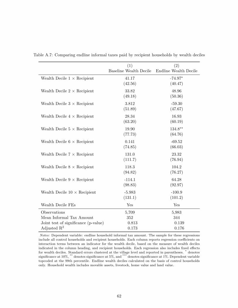
Table A.7: Comparing endline informal taxes paid by recipient households by wealth deciles

(1) (2)Baseline Wealth Decile Endline Wealth Decile

Wealth Decile 1 × Recipient 41.17 -74.97∗

(42.56) (40.47)

Wealth Decile 2 × Recipient 33.82 48.96(49.18) (50.36)

Wealth Decile 3 × Recipient 3.812 -59.30(51.89) (47.67)

Wealth Decile 4 × Recipient 28.34 16.93(63.20) (60.19)

Wealth Decile 5 × Recipient 19.90 134.8∗∗

(77.73) (64.76)

Wealth Decile 6 × Recipient 0.141 -69.52(74.85) (66.03)

Wealth Decile 7 × Recipient 131.0 23.32(111.7) (76.94)

Wealth Decile 8 × Recipient 118.3 104.2(94.82) (76.27)

Wealth Decile 9 × Recipient -114.1 64.28(98.83) (92.97)

Wealth Decile 10 × Recipient -5.983 -100.9(131.1) (101.2)

Wealth Decile FEs Yes Yes

Observations 5,709 5,983Mean Informal Tax Amount 352 344Joint test of significance (p-value) 0.813 0.139Adjusted R2 0.173 0.176

Notes: Dependent variable: endline household informal tax amount. The sample for these regressionsinclude all control households and recipient households. Each column reports regression coefficients oninteraction terms between an indicator for the wealth decile, based on the measure of wealth decilesindicated in the column heading, and recipient households. Each regression also includes fixed effectsfor wealth deciles. Standard errors clustered at the village level and reported in parentheses. * denotessignificance at 10%, ** denotes significance at 5%, and *** denotes significance at 1%. Dependent variabletopcoded at the 99th percentile. Endline wealth deciles calculated on the basis of control householdsonly. Household wealth includes movable assets, livestock, home value and land value.

62

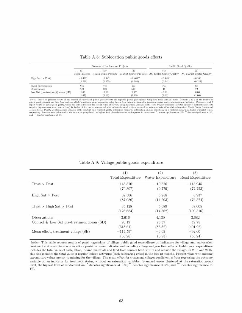
Table A.8: Sublocation public goods effects

Number of Sublocation Projects Public Good Quality

(1) (2) (3) (4) (5)Total Projects Health Clinic Projects Market Center Projects AC Health Center Quality AC Market Center Quality

High Sat (× Post) −0.392∗ 0.142 −0.469∗∗ −0.443∗ −0.100(0.226) (0.255) (0.180) (0.241) (0.217)

Panel Specification Yes Yes Yes No NoObservations 549 321 510 46 72Low Sat (pre-treatment) mean (SD) 1.06 0.68 0.67 −0.00 0.00

(1.47) (1.02) (1.03) (1.00) (1.00)

Notes: This table presents results on the number of sublocation public good projects and reported public good quality, using data from assistant chiefs. Columns 1 to 3 on the number ofpublic goods projects use data from assistant chiefs to estimate panel regressions using interactions between sublocation treatment status and a post-treatment indicator. Columns 4 and 5report results on public good quality, which was only collected in the second round of surveys, using data from assistant chiefs. Total Projects measures the total number of sublocation projects(repairs, improvements, new constructions) for health clinics, market centers and other sublocation-level projects reported by assistant chiefs within their sublocation. Health Center Quality andMarket Center Quality are standardized variables of the assistant chief-reported quality of facilities within the sublocation, and are conditional on a sublocation having a health or market center,respectively. Standard errors clustered at the saturation group level, the highest level of randomization, and reported in parentheses. * denotes significance at 10%, ** denotes significance at 5%,and *** denotes significance at 1%.

Table A.9: Village public goods expenditure

(1) (2) (3)Total Expenditure Water Expenditure Road Expenditure

Treat × Post −148.870∗ −10.876 −118.945(79.307) (9.779) (72.253)

High Sat × Post 32.306 3.258 6.937(87.086) (14.203) (76.524)

Treat × High Sat × Post 35.128 5.689 38.005(128.684) (14.362) (109.316)

Observations 3,616 4,130 3,882Control & Low Sat pre-treatment mean (SD) 93.19 23.37 49.75

(518.61) (83.32) (401.92)Mean effect, treatment village (SE) −114.59∗ −6.03 −92.00

(63.26) (6.93) (58.24)

Notes: This table reports results of panel regressions of village public good expenditure on indicators for village and sublocationtreatment status and interactions with a post-treatment indicator and including village and year fixed effects. Public good expenditureincludes the total value of cash, labor, in-kind materials and land from sources both within and outside the village. In 2015 and 2016,this also includes the total value of regular upkeep activities (such as clearing grass) in the last 12 months. Project-years with missingexpenditure values are set to missing for the village. The mean effect for treatment villages coefficient is from regressing the outcomevariable on an indicator for treatment status, without an saturation variables. Standard errors clustered at the saturation grouplevel, the highest level of randomization. * denotes significance at 10%, ** denotes significance at 5%, and *** denotes significance at1%.

63

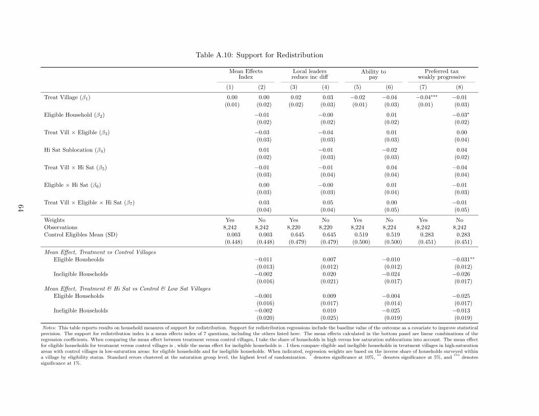
Table A.10: Support for Redistribution

Mean EffectsIndex

Local leadersreduce inc diff

Ability topay

Preferred taxweakly progressive

(1) (2) (3) (4) (5) (6) (7) (8)

Treat Village (β1) 0.00 0.00 0.02 0.03 −0.02 −0.04 −0.04∗∗∗ −0.01(0.01) (0.02) (0.02) (0.03) (0.01) (0.03) (0.01) (0.03)

Eligible Household (β2) −0.01 −0.00 0.01 −0.03∗

(0.02) (0.02) (0.02) (0.02)

Treat Vill × Eligible (β3) −0.03 −0.04 0.01 0.00(0.03) (0.03) (0.03) (0.04)

Hi Sat Sublocation (β4) 0.01 −0.01 −0.02 0.04(0.02) (0.03) (0.03) (0.02)

Treat Vill × Hi Sat (β5) −0.01 −0.01 0.04 −0.04(0.03) (0.04) (0.04) (0.04)

Eligible × Hi Sat (β6) 0.00 −0.00 0.01 −0.01(0.03) (0.03) (0.04) (0.03)

Treat Vill × Eligible × Hi Sat (β7) 0.03 0.05 0.00 −0.01(0.04) (0.04) (0.05) (0.05)

Weights Yes No Yes No Yes No Yes NoObservations 8,242 8,242 8,220 8,220 8,224 8,224 8,242 8,242Control Eligibles Mean (SD) 0.003 0.003 0.645 0.645 0.519 0.519 0.283 0.283

(0.448) (0.448) (0.479) (0.479) (0.500) (0.500) (0.451) (0.451)

Mean Effect, Treatment vs Control VillagesEligible Housheolds −0.011 0.007 −0.010 −0.031∗∗

(0.013) (0.012) (0.012) (0.012)Ineligible Households −0.002 0.020 −0.024 −0.026

(0.016) (0.021) (0.017) (0.017)Mean Effect, Treatment & Hi Sat vs Control & Low Sat Villages

Eligible Households −0.001 0.009 −0.004 −0.025(0.016) (0.017) (0.014) (0.017)

Ineligible Households −0.002 0.010 −0.025 −0.013(0.020) (0.025) (0.019) (0.019)

Notes: This table reports results on household measures of support for redistribution. Support for redistribution regressions include the baseline value of the outcome as a covariate to improve statisticalprecision. The support for redistribution index is a mean effects index of 7 questions, including the others listed here. The mean effects calculated in the bottom panel are linear combinations of theregression coefficients. When comparing the mean effect between treatment versus control villages, I take the share of households in high versus low saturation sublocations into account. The mean effectfor eligible households for treatment versus control villages is , while the mean effect for ineligible households is . I then compare eligible and ineligible households in treatment villages in high-saturationareas with control villages in low-saturation areas: for eligible households and for ineligible households. When indicated, regression weights are based on the inverse share of households surveyed withina village by eligibility status. Standard errors clustered at the saturation group level, the highest level of randomization. * denotes significance at 10%, ** denotes significance at 5%, and *** denotessignificance at 1%.

64

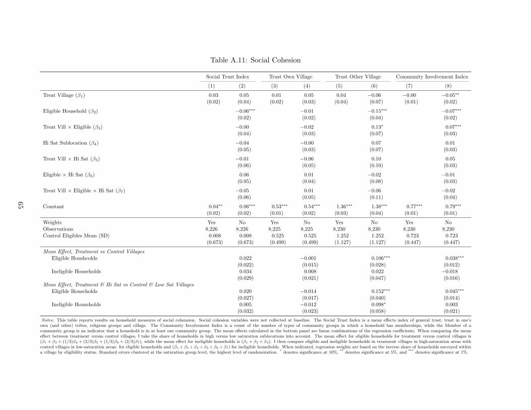
Table A.11: Social Cohesion

Social Trust Index Trust Own Village Trust Other Village Community Involvement Index

(1) (2) (3) (4) (5) (6) (7) (8)

Treat Village (β1) 0.03 0.05 0.01 0.05 0.04 −0.06 −0.00 −0.05∗∗

(0.02) (0.04) (0.02) (0.03) (0.04) (0.07) (0.01) (0.02)

Eligible Household (β2) −0.06∗∗∗ −0.01 −0.15∗∗∗ −0.07∗∗∗

(0.02) (0.02) (0.04) (0.02)

Treat Vill × Eligible (β3) −0.00 −0.02 0.13∗ 0.07∗∗∗

(0.04) (0.03) (0.07) (0.03)

Hi Sat Sublocation (β4) −0.04 −0.00 0.07 0.01(0.05) (0.03) (0.07) (0.03)

Treat Vill × Hi Sat (β5) −0.01 −0.06 0.10 0.05(0.06) (0.05) (0.10) (0.03)

Eligible × Hi Sat (β6) 0.06 0.01 −0.02 −0.01(0.05) (0.04) (0.08) (0.03)

Treat Vill × Eligible × Hi Sat (β7) −0.05 0.01 −0.06 −0.02(0.06) (0.05) (0.11) (0.04)

Constant 0.04∗∗ 0.06∗∗∗ 0.53∗∗∗ 0.54∗∗∗ 1.36∗∗∗ 1.38∗∗∗ 0.77∗∗∗ 0.79∗∗∗

(0.02) (0.02) (0.01) (0.02) (0.03) (0.04) (0.01) (0.01)

Weights Yes No Yes No Yes No Yes NoObservations 8,226 8,226 8,225 8,225 8,230 8,230 8,230 8,230Control Eligibles Mean (SD) 0.008 0.008 0.525 0.525 1.252 1.252 0.723 0.723

(0.673) (0.673) (0.499) (0.499) (1.127) (1.127) (0.447) (0.447)

Mean Effect, Treatment vs Control VillagesEligible Housheolds 0.022 −0.001 0.106∗∗∗ 0.038∗∗∗

(0.022) (0.015) (0.028) (0.012)Ineligible Households 0.034 0.008 0.022 −0.018

(0.029) (0.021) (0.047) (0.016)Mean Effect, Treatment & Hi Sat vs Control & Low Sat Villages

Eligible Households 0.020 −0.014 0.152∗∗∗ 0.045∗∗∗

(0.027) (0.017) (0.040) (0.014)Ineligible Households 0.005 −0.012 0.098∗ 0.003

(0.032) (0.023) (0.058) (0.021)

Notes: This table reports results on household measures of social cohension. Social cohesion variables were not collected at baseline. The Social Trust Index is a mean effects index of general trust, trust in one’sown (and other) tribes, religious groups and village. The Community Involvement Index is a count of the number of types of community groups in which a household has memberships, while the Member of acommunity group is an indicator that a household is in at least one community group. The mean effects calculated in the bottom panel are linear combinations of the regression coefficients. When comparing the meaneffect between treatment versus control villages, I take the share of households in high versus low saturation sublocations into account. The mean effect for eligible households for treatment versus control villages is(β1 + β3 + (1/3)β4 + (2/3)β5 + (1/3)β6 + (2/3)β7), while the mean effect for ineligible households is (β1 + β3 + β4). I then compare eligible and ineligible households in treatment villages in high-saturation areas withcontrol villages in low-saturation areas: for eligible households and (β1 + β3 + β4 + β5 + β6 + β7) for ineligible households. When indicated, regression weights are based on the inverse share of households surveyed withina village by eligibility status. Standard errors clustered at the saturation group level, the highest level of randomization. * denotes significance at 10%, ** denotes significance at 5%, and *** denotes significance at 1%.

65

B Additional details on data collection and intervention

This section contains additional details on the data collection, study context and program interven-

tion by GiveDirectly. Tables B.1 and B.2 document the high tracking rates achieved by both the

household and local leader surveys across rounds. Table B.3 provides details on the range of village

sizes and its implications for the share of households surveyed in each village. Table B.4 documents

how Siaya compares to other parts of Kenya, using data from the 2009 Kenya Population and

Housing Census. This census took place prior to devolution and the establishment of the county

system of government; instead, data is aggregated to the district level. The study area is located

entirely within the former Siaya district, and I compare Siaya district with the other districts in

existence at the time of the 2009 census.

Section B.1 outlines the steps in GD’s enrollment process in more detail, and provides figures

on the rollout of transfers over time, as well as a map documenting the spatial distribution of

transfers.

66

Table B.1: Household survey tracking rates

Share Surveyed Share of endline surveys baselinedTargets Num. Surveys Mean T vs C (S.E.) Num. Surveys Mean T vs C (S.E.)

All Households 9,150 8,242 0.901 0.006 7,845 0.877 -0.003(0.006) (0.007)

Eligible Households 6,039 5,425 0.898 0.005 5,196 0.879 -0.005(0.008) (0.009)

Ineligible Households 3,111 2,817 0.905 0.007 2,649 0.873 0.001(0.010) (0.013)

Notes: This table reports endline household survey tracking rates, both overall and by eligibility status. Column 1 reports the total number of householdstargeted for endline surveys; this includes households that were “initially sampled” at baseline and “replacement” baseline households. Columns 2 and 5 reportthe number of endline and baseline surveys conducted, respectively. Columns 3 and 4 present the share of households targeted for endline surveys that weresurveyed, while columns 6 and 7 present the share of households surveyed at endline that were also surveyed at baseline. Columns 4 and 7 report t-tests fordifferences in means by village treatment status, with standard errors in parentheses, and show that tracking rates are balanced across treatment and controlvillages both overall and by eligibility status. * denotes significance at 10%, ** denotes significance at 5%, and *** denotes significance at 1%.

67

Table B.2: Local leader tracking rates

Round 1 Round 2Share Surveyed Share Surveyed

Targets Surveyed Mean

T - C /

Hi - Low (SE) Targets Surveyed Mean

T - C /

Hi - Low (SE)

Villages (Village Elders)a 653 633 0.969 0.013 653 640 0.980 -0.021*

(0.013) (0.011)Sublocations (Assistant Chiefs) 84 84 1.000 0.000 84 84b 1.000 0.000

(0.000) (0.000)a: Numbers reported at the GE village level, which corresponds to census enumeration areas. In some cases more than one village elder was surveyed per GEvillage.b: 73 assistant chiefs were tracked during the main second round local leader survey period from July to December 2016 (an 87 percent tracking rate). The 11assistant chiefs missed during this period were successfully surveyed from January to July 2017. Tracking rates remain balanced across treatment status whenexcluding these later surveys.Notes: This table reports local leader survey tracking rates. Columns 1 through 4 report on the first round of local leader surveys, conducted from July toDecember 2015, while columns 5 through 8 report on the second round, conducted from July to December 2016. Columns 1 and 5 report the total targetnumber of villages and sublocations; this comprises the total number in our study. Columns 2 and 6 report the number of surveys conducted in each round,while columns 3 and 7 report tracking rates by round. Columns 4 and 8 report t-tests for differences in means; at the village level, this tests for differences insurvey rates for treatment versus control villages. At the sublocation level, this tests for differences in high saturation sublocations versus low saturationsublocations. Standard errors are reported in parentheses. * denotes significance at 10%, ** denotes significance at 5%, and *** denotes significance at 1%.

68

Figure B.1: Share of households eligible for GD transfers by village

0

1

2

3

4D

ensi

ty

0 .1 .2 .3 .4 .5 .6Proportion Eligible

Treatment Control

Source: GE baseline household census data (conducted 2014-15).Notes: This figure plots kernel densities of the share of households eligible for GD transfers by village, based on datacollected by the GE project household census in advance of the distribution of transfers. Eligible households arethose with a grass-thatched roof. A Kolmogorov - Smirnov test for the equality of distributions cannot reject that thedistributions are the same, indicating that the share of eligible households is balanced across treatment and controlvillages (p-value 0.913).

69

Table B.3: Village-Level Population, Survey Numbers and Shares

Mean (SD) Median Min Max

Panel A: Census DataNumber of households 100.13 98.00 19.00 245.00

(32.29)Proportion of eligible (thatched-roof) households 0.33 0.33 0.06 0.64

(0.10)Panel B: Baseline DataNumber of households surveyed at baseline 12.01 12.00 9.00 24.00

(0.58)Proportion of households surveyed at baseline 0.13 0.12 0.05 0.63

(0.05)Number of eligible households surveyed at baseline 7.90 8.00 4.00 12.00

(0.64)Proportion of eligible households surveyed at baseline 0.30 0.26 0.08 1.00

(0.16)Number of ineligible households surveyed at baseline 4.12 4.00 1.00 12.00

(0.70)Proportion of ineligible households surveyed at baseline 0.07 0.07 0.01 0.45

(0.04)Panel C: Endline DataNumber of households surveyed at endline 12.62 12.00 8.00 25.00

(1.82)Proportion of households surveyed at endline 0.14 0.13 0.06 0.68

(0.06)Number of eligible households surveyed at endline 8.31 8.00 4.00 16.00

(1.40)Proportion of eligible households surveyed at endline 0.31 0.26 0.08 1.00

(0.18)Number of ineligible households surveyed at endline 4.31 4.00 1.00 9.00

(0.96)Proportion of ineligible households surveyed at endline 0.07 0.07 0.01 0.45

(0.04)

Observations 653

Notes: This table reports village-level summary statistics on the number of households and the share of eligiblehouseholds from baseline household census data (Panel A), the number and share of households surveyed at baseline,by eligibility status (Panel B), and the number and share of households surveyed at endline, by eligibility status. Thebaseline household census and survey were conducted from August 2014 to August 2015, in advance of the distributionof transfers to each village. The baseline household survey targeted 12 households per village, 8 eligible householdsand 4 ineligible households. In case a household could not be surveyed, it was replaced by a randomly-selectedhousehold within the village. In one village, we surveyed 24 households; this village contained 2 that were mistakenlytreated as separate villages during the baseline census and survey. In another village, we targeted 18 households, asafter the baseline survey was conducted, we realized that an enumerator input an incorrect village at the time of thecensus, leading to the exclusion of these households from the sampling frame. We randomly sampled six householdsfrom these missed households to survey. The endline household survey was conducted from May 2016 to May 2017.The endline household survey targeted households surveyed at baseline, as well as households that were unable to besurveyed at baseline.

70

Table B.4: Comparison of demographic and economic indicators for study region and Kenyandistricts

Nationwide county percentiles

Siaya 25th 50th 75th

Total population 545,580 138,840 215,060 316,660Pct. rural 0.93 0.70 0.83 0.96Pct. attending school 0.39 0.33 0.39 0.42Pct. completed primary school 0.38 0.27 0.40 0.48Pct. completed secondary school 0.06 0.06 0.08 0.13Unemployment rate 0.30 0.33 0.39 0.43

Total households 133,830 29,170 43,410 73,390Pct. owns home 0.89 0.74 0.84 0.91Pct. with high quality floor 0.26 0.18 0.29 0.45Pct. with high quality walls 0.30 0.19 0.29 0.45Pct. with high quality roof 0.62 0.51 0.82 0.93Pct. with electricity 0.04 0.03 0.07 0.16Pct. with sewage disposal 0.01 0.00 0.01 0.04

The study region column presents weighted-average statistics for Siaya district and the 25th,50th, and 75th percentiles of 155 districts in Kenya. Demographic data is obtained from the 2009Kenya Population and Housing Census. High quality roof indicates roofs are made of concrete,tiles, or corrugated iron sheets. High quality floor indicates floors made of cement, tiles, orwood. High quality walls indicates walls made of stone brick, or cement.

71

B.1 GD’s Program

GD’s enrollment process in treatment villages consists of the following 6 steps:

1. Village Meeting (baraza): before beginning work in a village, GD holds a meeting of all

households in the village to inform villagers that GD will be working in their village, explain

their program and GD as an organization. To prevent gaming, the eligibility criteria are not

disclosed.53

2. Census: GD staff conduct a household census of the village, collecting information on house-

hold names, contact information and housing materials. The information on housing materials

are used to determine program eligibility.

3. Registration: Households identified as eligible based on the household census are visited by

the registration team. GD staff confirm the eligibility of the household, inform the household

of their eligibility for the program and register the household for the program. This is the

point at which households learn they will be receiving transfers, as well as the amount of the

transfers, the transfer schedule, and the fact that the transfer is unconditional.54 For couples,

the couple decides which individual will be designated as the recipient. The member of the

household identified as the recipient is instructed to register for M-Pesa in their name, a

prerequisite for receiving the transfer. Households that do not have a mobile phone are given

the option to purchase one from GD staff, the cost of which is deducted from the transfer

amount. Even if the household does not own a phone, the individual recipient can still register

for M-Pesa with a SIM card; the SIM card can then be inserted into any phone in order to

make withdrawals.

4. Backcheck: All registered households are backchecked to confirm eligibility in advance of the

transfers going out. This is an additional step to prevent gaming by households and field

staff, as the census, registration and backcheck teams consist of separate staff members.

5. Transfers: The cash is transferred in a series of three payments via M-Pesa according to the

following schedule: (i) the token transfer of KSH 7,000 (about USD 70) ensures the system

is working properly; (ii) two months afterwards, the first lump sum transfer of KSH 40,000 is

distributed; (iii) six months after this, the second and final lump sum transfer of KSH 40,000

is sent.55 Transfers are typically sent at one time per month to all households scheduled to

receive transfers.

53. However, the eligibility criteria is not difficult to deduce given that it is publicly observable, and anecdotallymany households in the study area are aware of targeting criteria.

54. To emphasize the unconditional nature of the transfer, households are provided a brochure with many potentialuses of the transfer.

55. If households elected to receive a mobile phone from GD, the cost of this is taken out of the second lump sumtransfer.

72

6. Follow-up: After transfers go out, GD staff follow up via phone with transfer recipients to

ensure no problems have arisen. In addition, there is a GD help line that recipients can

contact. If GD staff learn that household conflicts have arisen as a result of the transfers,

subsequent transfers may be delayed while these conflicts are worked out.

Figures B.2 documents that transfers began at roughly the same time for most households

within a village. Most households began receiving transfers within 3 months of the first transfer

being distributed to a village. B.3 displays the distribution of all three transfers across villages,

again showing that most households received their second and third transfers 2 and 6 months after

the first household within the village began receiving transfers.

Figure B.2: Proportion of first transfers made within villages

0.2

.4.6

.81

Prop

. of t

oken

tran

sfers

mad

e

0 10 20 30Months since first token transfer

Notes: This figure plots the proportion of first transfers made as a function of months since thefirst token transfer in each village. Each point represents cumulative mean proportion of transfersmade (relative to the number of eligible households within a village) by month, averaged acrossvillages. Error bars represent 95% confidence intervals.

73

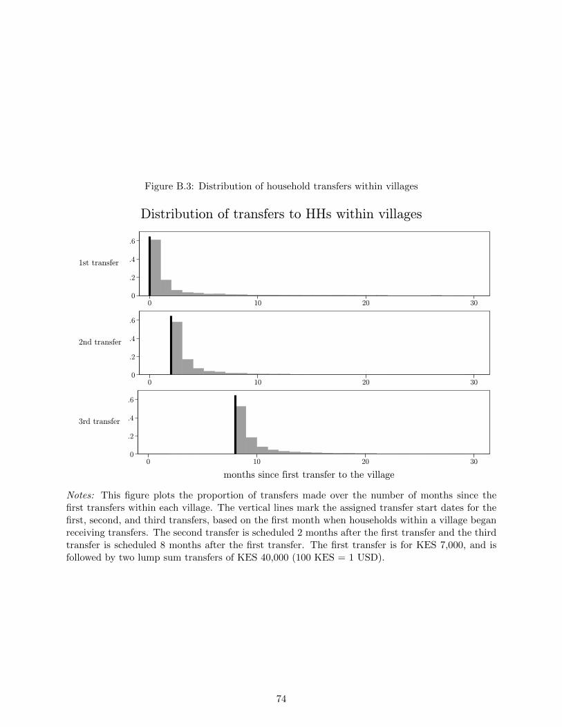
Figure B.3: Distribution of household transfers within villages

0

.2

.4

.6

1st transfer

0 10 20 30

0

.2

.4

.6

2nd transfer

0 10 20 30

0

.2

.4

.6

3rd transfer

0 10 20 30

months since first transfer to the village

Distribution of transfers to HHs within villages

Notes: This figure plots the proportion of transfers made over the number of months since thefirst transfers within each village. The vertical lines mark the assigned transfer start dates for thefirst, second, and third transfers, based on the first month when households within a village beganreceiving transfers. The second transfer is scheduled 2 months after the first transfer and the thirdtransfer is scheduled 8 months after the first transfer. The first transfer is for KES 7,000, and isfollowed by two lump sum transfers of KES 40,000 (100 KES = 1 USD).

74

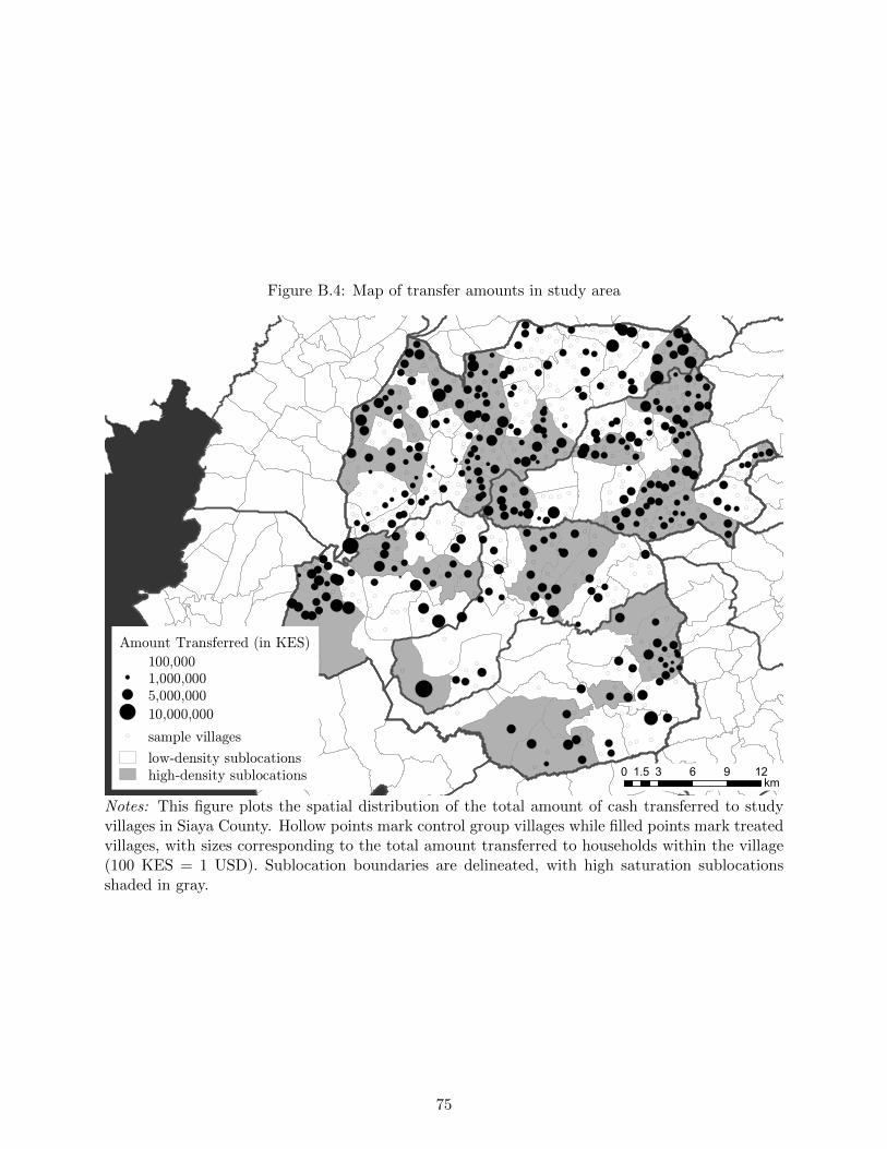
Figure B.4: Map of transfer amounts in study area

(

(

(

(

(

(

(

(

( (

(

(

(

(

(( (

(

(

(

(

((

(

(

(

(

(

(

(

((

(

(

((

( (

(

(

(

(

(

(

((

(

(

(

(

(

(

(

(

(

(

((

(

(

((

((

((

(

(

(

((

( (

((

(

(

(

(

(

( (

(

(

((

(

(

((

(

( (

((

(

(

( (

((

(

(

((

((

((

((

(((

((

((

((

(

(

(

( (

(((

((

(

(

((

(

(

(

((

(

(

((

((

(

(

(

((

((

(

(

((

( (

((

(

( ((

(

(

(

(

(

(

((

(

(

(

((

((

((

(

(

(

(

(

(

(

( (

(

(

( (

((

(

((

(

((

(

((

(

((

(

(((

(

(

((

((

(

(

(

(

((

(

((

( (

(( (

(

(

((

(

((

(

(

(

(

((

((

(

(((

((

(

(

(

(

(

((

(

(

(

(

(

( (

(

((

(

(

(

(

(

(

( (

((

(

(

((

(

(

(

(

(

( (

(

((

((

(

(

(

(

(

(

(

(

(

((

(

(

( (

(

(

(

((

(

( (

(

(

(

(

(

(

((

(

(

(

(

(

(

(

(

(

((

(

(

((

((

(

(

((

(

(

(

(

(

(

((

(

(

((

(

(

( (( ( (

(

(

(

(

(

((

((

(

(

((((

(

((

( (

(

(

(

(

(

(

( ((

((

((

(

(

(

(

(

(((

(

(

(

(

( ((

(

(

(

(

(

(

(

(

(

( (( (

((

((

(((

(

((( (

((

(

(

(

((

( (( ( (

(

(

((

(

(

(

( ((

(

(

(

(

((

((

(

(

(((

(

(

(

(

( (

(

(

(

(

(

(

( ( ((

(((

( (

(

((

(

((

(

(

(

(

((

(

(

((

( ( (

((

(

( ( ( ((

(

((

(( (

(

((

(((

( (

(

(

(

((

( (

(( (

((

(

(((

(

((

(

(

( (

(

(( (

(

(

(

( (

((

((

((

(

((

(

(

( (

((

(

((

(

((

( (

((

(

(

( ((

((

(

(

(

(

((

(

((

(

( ((

(

((

((

(

(((

(

(

(

(( (

(

((

((

(

(

(((

((

(

( (

(

((

(

(

(

(

(

(

Amount Transferred (in KES)100,0001,000,0005,000,00010,000,000

( sample villageslow-density sublocationshigh-density sublocations 0 3 6 9 121.5 km

Notes: This figure plots the spatial distribution of the total amount of cash transferred to studyvillages in Siaya County. Hollow points mark control group villages while filled points mark treatedvillages, with sizes corresponding to the total amount transferred to households within the village(100 KES = 1 USD). Sublocation boundaries are delineated, with high saturation sublocationsshaded in gray.

75