Informal Taxation and Cash Transfers: Experimental Evidence

from Kenya∗

Michael WalkerUC Berkeley

October 13, 2017

Link to most recent versionPlease do not cite without author permission

Abstract

Informal taxation plays an important role in local public good provision in many developingcountries, yet little is known about how informal taxation responds to income growth. Informaltaxation is implemented by local leaders with better information on household income thanthe government, so one may expect taxes to be highly responsive. This paper uses exogenousvariation in household income from a large-scale randomized controlled trial of a one-time un-conditional cash transfer program to study how informal taxation and public goods provisionresponds to household income shocks. The cash transfer program is both large in scale and per-household amounts: almost USD 11 million was distributed to poor households in 653 villagesin rural Kenya, and comprise 75 percent of annual consumption expenditure for recipient house-holds. I find the transfers have no effect on household informal tax payments despite the factlocal leaders are knowledgable about the households receiving transfers, and no effect on publicgoods provision. Household formal tax payments increase slightly. Overall, the magnitude ofthe tax effects are small: I estimate an increase in total taxes of 0.7 to 2.2 percent of the totalamount transferred into the study area, depending on the specification used. I find that informaltax payments by recipient households are not based on their (temporarily) higher income fromthe cash transfers, but instead in line with their pre-treatment income. This flexibility suggestsan equity advantage of informal taxation (as compared to formal taxes) in high income-volatilityenvironments.

∗Email: mwwalker@econ.berkeley.edu. Thanks to Justin Abraham, Dennis Egger, Gabriel Ngoga, Meshack Okello,Priscila de Oliveira, Francis Wong and Zenan Wang for excellent research assistance, IPA-Kenya for data collec-tion, and GiveDirectly for collaboration. Thanks to Ted Miguel, Johannes Haushofer, Paul Niehaus, Lauren FalcaoBergquist, Ben Faber, Fred Finan, Supreet Kaur, Monica Singhal, Danny Yagan and seminar participants at theWGAPE Fall 2016 meetings and UC Berkeley for feedback. This work has been funded by the Private EnterpriseDevelopment in Low-Income Countries (PEDL) initiative, the International Growth Centre, the Weiss Family Foun-dation, and an anonymous donor. I gratefully acknowledges financial support from the National Science FoundationGraduate Research Fellowship (Grant No. DGE 1106400).

1

1 Introduction

A central question in public economics is how to fund public goods. In many developing countries,

informal taxation, whereby local public goods financing is coordinated by local officials and enforced

socially rather than through the formal legal system, plays an important role in funding public

goods (Olken and Singhal 2011). Informal taxation can offer some benefits relative to formal

taxation in village economies. Local leaders are likely better informed about both village needs

and households’ income and earnings abilities than the government. By not having a fixed tax

schedule they also offer greater flexibility than a formal tax system. It also provides a source of

locally controlled revenue. However, local leaders have less enforcement capacity than the state, as

they rely on social sanctions. In cases where local leaders are unelected, there is the potential for

less accountability and elite capture.

Yet, we still know relatively little about informal taxation (DFID 2013), how households are

targeted for payments and in particular how these payments respond to household income growth,

as the (limited) existing evidence documents stylized facts in the cross-section (Olken and Singhal

2011). In this paper, I use detailed panel data on both households and local leaders to explore

the relationship between income changes and informal taxation. I then provide causal estimates

on the response of informal taxation and public goods to an exogenous shock to household income

generated by an RCT of a large one-time unconditional cash transfer program.

Unconditional cash transfers (UCTs) have been growing in popularity as a tool for economic

development and poverty alleviation and are scaling rapidly both worldwide and in sub-Saharan

Africa.1 Proponents of unconditional cash transfers appreciate that i) they allow recipients to spend

money as they find most effective, providing a greater range of options for recipients than in-kind

aid programs; ii) they have low administrative costs because there is no need for procurement,

training, or monitoring, so a greater proportion of funds can be provided as direct assistance

(Margolies and Hoddinott 2015); and iii) a large set of existing evidence finds positive benefits for

recipient households (Arnold, Conway, and Greenslade 2011) and that households do not spend

transfers on temptation goods (Evans and Popova 2014). Relatively little is known about the

interaction between cash transfer programs and local public finance in developing countries, where

informal local institutions can play a key role in both funding and maintaining local public goods.

If a portion of unconditional cash transfers to households is channeled into public good investments,

this provides a mechanism for both long-term benefits and spillover benefits to non-recipients from

a one-time transfer. As cash transfers continue to scale rapidly (Faye, Niehaus, and Blattman

2015), this is an important policy question.

1. For instance, Kenya partnered with the World Bank in 2013 to develop the National Social Safety Net Pro-gram for Results, which combines and expands cash transfer programs (http://www.worldbank.org/en/news/press-release/2013/07/23/world-bank-help-kenya-build-national-safety-net), Liberia is starting a cashtransfer program for 10,500 households affected by Ebola (http://allafrica.com/stories/201502060847.html)and Ghana announced an expansion of a cash transfer program for pregnant women and young children in March2015 (http://allafrica.com/stories/201503051428.html).

2

The NGO GiveDirectly (GD) makes large unconditional cash transfers to poor households

in Kenya. The magnitude of the transfers is large, around US$1,000 (nominal) per household,

about 75% of annual expenditure for recipient households. For this study, GD targets households

living in homes with grass-thatched roofs, a basic means-test for poverty, which is publicly observ-

able. The intervention involves almost US$11 million in transfers and 653 villages in one Kenyan

county. Treatment assignment is randomized at the village level, and within treatment villages, all

households meeting GD’s eligibilty requirement receive the unconditional cash transfer.

One might expect the greatest potential for public good investment to come when transfers

are based on criteria that are known and observable to others, and when transfers are distributed at

the same point in time for many households, as this help solve both information and coordination

challenges for local leaders. Both of these aspects are present in this study. GD informed local

leaders prior to the start of their operations within a village, and while the targeting criteria of

grass-thatched roofs was not disclosed in advance, this is publicly observable for households within

the village and was easy for villagers to deduce which households received transfers.In addition,

while transfers were distributed over a set of 3 payments, over 90 percent of recipient households

received their payments within 3 months of the first household within the village receiving a transfer.

The detailed data I collect allows me to document a number of important patterns related

to the funding of local public goods in rural Kenya. I first show that in the cross-section, informal

taxation provides an important source of locally-controlled funding, and that while informal tax

participation and payments are increasing in income, higher income households pay less as a share

of income, implying that informal taxation is regressive. These are both consistent with findings by

Olken and Singhal (2011). I use the panel nature of my household data to show that as households

in control villages move up or down the income or wealth distribution, the amount they pay in

informal taxes changes.

I then turn my attention to the effects of the unconditional cash transfer intervention. Re-

cipient households do indeed benefit from the transfers - eligible households in treatment villages

(an ITT estimate) see an increase in household asset ownership of 40 percent and an increase

in consumption of 12 percent on average 18 months after the start of transfers (Haushofer et al.

2017). Recipient households are also 4 percentage points (on a base of 46 percent) more likely to

be self-employed.

However, I find no significant effect on the amount of informal taxes paid by recipient or

non-recipient households, nor on their likelihood of paying informal taxes. I do find that recipient

households pay more in formal taxes associated with self-employment. Non-recipient households

in treatment villages also pay more in national income taxes, though only 3 percent of households

report paying any income taxes. Overall, the effects on both formal and informal taxes are small:

the point estimates on the total amount paid in taxes suggest an increase of 0.7 to 2.2 percent

of the total amount of the UCT program. This suggests that there is not elite capture whereby

transfer recipients are overtaxed by local leaders.

3

Next, I document effects on public good provision. Perhaps unsurprisingly given the lack

of an effect on informal taxes, I find no increase in the number of public goods projects, public

good expenditure or reported public good quality in treatment villages. These results present a

puzzle, as typical models of public good provision would suggest either a) an increase in taxes,

spending and public good provision as household income increases or b) if leaders are funding

a fixed quantity of public goods, an increase in taxes for recipient households and a decrease in

taxes for non-recipient households. I show that leaders are taxing recipient households at a similar

rate to control households with the same baseline income, rather than at recipient household’s

post-treatment earned income or earned plus UCT transfer income. This is consistent with leaders

recognizing the one-time nature of the income shock, and the fact the transfers are targeted at

poorer households, who may otherwise have more limited earnings potential. While the windfall

income leads households to have temporarily high annual income, it has a much smaller effect on

household’s permanent income. Leaders thus exercise discretion and tax households more similarly

to their pre-treatment rates. This highlights an equity benefit of informal taxation relative to

formal taxation, such as in the US, where any windfall income counts towards a households’ yearly

tax rate. In settings where income can be highly volatile, this suggests an additional appeal of

informal taxation.

These findings shed additional light on the costs and benefits of informal institutions (e.g.

Udry 1994; Jakiela and Ozier 2016). They also relate to the behavior of local leaders and tax

collectors: Alatas et al. (2012) find that local leaders use more information in targeting beneficiaries

of a one-time cash transfer, and appear to be targeting on the basis of more than just household

consumption. Khan, Khwaja, and Olken (2015) find that in response to additional incentives for

tax collection, collectors focus on a small number of high-value targets, rather than seeking to raise

smaller amounts of revenue from a larger number of people.

These results are also relevant to the policy implications of UCTs. In this context, transfers

do reach their intended targets and are not captured by local leaders, but these results suggest

that this one-time positive income shock does not translate into increased public goods investment,

turning off a potential channel for spillover benefits to non-recipient households.

The rest of this paper is organized as follows. Section 2 provides background information on

the informal and formal tax system in rural Kenya. Section 3.2 provides details on the intervention

and experimental design. Section 4 describes the survey data used in this paper. Section 5 describes

the empirical specifications used to estimate the results presented in Section 6. Section 7 outlines

how recipient informal tax amounts are in line with baseline income and Section 8 concludes.

4

2 Local public finance in rural Kenya

This section describes the formal and informal taxes to which households in Kenya are subject, and

the manner in which these taxes are collected.2

I first make use of my unique panel data on households and public goods to characterize the

nature of informal taxation in rural Kenya.3 I provide a brief overview of the study setting, the

local leaders that are collecting informal taxes, the types of public goods they are funding, and the

implications for households (how much households pay, what types of households pay). I document

three key facts. First, while informal taxation may make up a small share of household income, it

provides an important source of locally-controlled funding for local public goods. Second, informal

tax amounts are increasing in household income and wealth, but regressive. These first two facts

echo findings from Olken and Singhal (2011). In addition, conditional on income or wealth, select

groups pay different amounts; for example, on average, widows pay less than predicted by their

income level, and households with greater education pay more. Third, the amount paid in informal

taxes responds to changes in household income and wealth.

2.1 Study Setting

This study takes place in Siaya County, Kenya, a populous rural area in western Kenya border-

ing Lake Victoria. Siaya County is predominatly Luo, the second-largest ethnic group in Kenya.4

Kenya offers a particularly interesting opportunity to look at informal taxaation for several reasons.

It has a long tradition of local fundraising for public goods through community meetings. Known

as harambees, these public ceremonies for local fundraising have played a central role in develop-

ment policy since independence; 90% of respondents in rural central Kenya in 1980 had contributed

(Barkan and Holmquist 1986). While contributions are ostensibly voluntary, Miguel and Gugerty

(2005) document the many ways in which social pressure and sanctions are used to elicit contri-

butions, including writing letters to households, encouraging pastors to mention the importance of

contributing in church sermons, home visits, and public announcements of households that have

not fulfilled their contributions.

GD selected three subcounties within Siaya for expansion based on their high poverty lev-

els, and our sample includes all rural villages (those outside of town centers) in which GD had

not previously worked.5 This provided a total of 653 villages containing approximately 65,000

2. In all of the analysis that follows, I focus on direct taxation of households by the national and county governments,and local leaders. Most notably, this excludes indirect taxes such as the value-added tax and excise taxes on petrol;given the low rates of enterprise formality, it is unclear to what extent the incidence of these taxes are borneby households. This also excludes fees paid by households to schools for their children’s attendance, though notcontributions to school development projects, which I consider public goods projects.

3. Full details on the data are provided in Section 4.4. This paper is one component of a broader investigation into the general equilibrium effects of cash transfers (the

“GE” project) (Haushofer et al. 2014).5. In data from the 2009 Kenyan census, Siaya is at or below the median on available development indicators (see

5

households.

Villages are the lowest administrative unit in Kenya, contain a mean of 100 households, and

range from a minimum of 19 households to a maximum of 245 (Table 13, Panel A). Villages are

overseen by a village elder (VE), an unsalaried position appointed by the assistant chief (AC).6

ACs adminster sublocations, the administrative unit directly above the village level; sublocations

in the study area contain an average of 10 villages. ACs are the lowest-level administrator that is

salaried by the national government and are appointed by chiefs (who administer locations). Due

to the governmental salary, appointment is competitive. There are no set term limits for either

VEs or ACs, and limited upward advancement within either position. Assistant chiefs and village

elders are required to be residents of the village / sublocation that they administer; typically these

are also the “home areas” where the leaders grew up and have longstanding familial ties. In what

follows, statements about “local leaders” refer to ACs and VEs jointly.

2.2 Informal taxation in rural Kenya

Local leaders are responsible for overseeing public goods within their area and promoting develop-

ment. However, local leaders do not receives a dedicated budget from the government, so they must

either find external funding or raise money from households within their jurisdiction via informal

taxation. To raise external funding, leaders can solicit funding from politician-led development

funds or NGOs.7 However, successfully receiving funding from external sources is highly uncertain:

in 2015, only 20 percent report receiving any funding from external sources, and external funding

can still require village co-funding. Local leaders thus collect informal taxes from households in

order to maintain, repair and improve public goods in their jurisdiction. Funding is typically raised

for a specific project or purpose. In this way, local leaders serve as “development brokers” (Bald-

win 2016). Local leaders thus consider the costs and benefits of a project to households in their

jurisdiction, their own effort costs and their own payoff (from households) of completing a project.

The urgency and amount of money to be collected will depend on situation on the ground.

Informal tax revenue collection can take a variety of forms. Leaders can hold a village meeting

to assign contributions, or, for larger projects, can hold a community fundraiser. Known as a

harambee, these events have invited “guests of honor” who are expected to make large contributions,

though all attendees are expected to contribute. Contributions are made in public, so they are

highly visible. Leaders can also go door-to-door for collections. Payment enforcement is on the

basis of social sanctions. Miguel and Gugerty (2005) document letter-writing campaigns, home

visits and public announcements for households that did not make expected contributions. Non-

payment can also result in exclusion from informal insurance arrangements, as leaders take past

Table 14).6. While the position is unsalaried, it does carry the potential for remuneration: for example, VEs frequently

receive an “appreciation” payment for their time when resolving disputes or serving as guides to NGO field workers.7. Both Members of Parliament (national-level politicians) and Members of the County Assembly (county-level

politicians) have development funds for use on projects in their constituencies.

6

contributions into account when deciding whether to take up collections for households for events

such as funerals or weddings.8

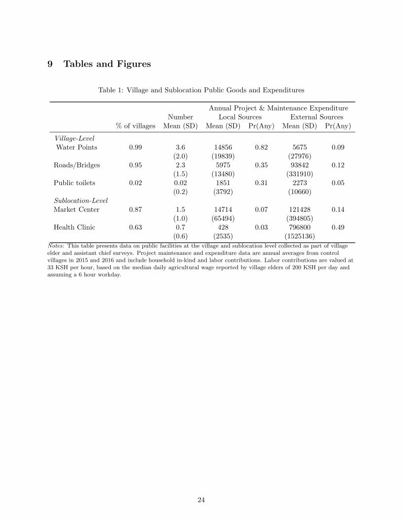
Given that local leaders do not have dedicated budgets, informal taxes serve as an important

source of locally-controlled revenue. This is especially true for public goods such as water points,

where, in an average year, over 2.5 times as much funding comes from informal taxes compared

to external sources (Table 1). Even for roads and bridges, while external sources provide more

funding on average in a year, only 12 percent of villages receive any outside road funding, leaving

local leaders to raise funding via informal taxes for basic repair and maintenance. In addition,

many of the projects undertaken by villages are small (Figure 1).

Now, I turn to the household side, and document cross-sectional patterns using pre-transfer

data. About half of all households report paying informal taxes in pre-treatment data. Panel A of

Figure 2 plots the household income distribution, where household income is defined as household

agricultural profits, self-employment profits and wage earnings. The gray vertical lines denote

income deciles, which I utilize in Panels B through D. Panel B plots the mean share of households

making any informal tax payments (in cash or labor) by income decile, while the bars plot the upper

and lower 95 percent confidence intervals. The share of households paying any informal taxes is

rising in income; likewise, the mean amount paid in informal taxes is also rising with income (Panel

C). The relationship between income deciles and informal tax amounts is positive but relatively

flat over the first 7 deciles, suggesting that the marginal informal tax on income may be relatively

small. In Panel D, we see that higher income households pay less in informal taxes as a share

of their income. There is likely measurement error and underreporting of income in this setting

(like many development settings), so the income shares may be overestimates. However, the fact

that informal taxes are regressive holds when using household wealth instead of income (Appendix

Figure A.1), and aligns with findings by Olken and Singhal (2011).9 Even at 1 to 2 percent of

household income, informal taxes would not be trivial for poor households, and these amounts fall

within the range found by Olken and Singhal (2011) across 10 countries.

Figures 2 and A.1 plot the relationship between informal taxes and income and wealth in

the cross-section. I now use households in control villages (where transfers were not distributed)

to look at how informal taxes change in response to household shifts in income and wealth deciles.

I estimate the following equation for both income and wealth on control households surveyed at

both baseline and endline:

∆InformalTaxhv = α+ ∆Decilehv + εhv (1)

where ∆InformalTaxhv subtracts the amount paid in baseline informal taxes from the amount

paid in informal taxes at endline. ∆Decilehv subtracts either the baseline income or wealth decile

8. Note that my results focus on collections for public goods.9. Interestingly, informal taxes as a share of household wealth are on the low end, but within the range, of typical

US property tax rates.

7

from the endline value, depending on the specification. I cluster standard errors at the village

level. Table 2 presents the results. A one decile increase in a household’s income or wealth decile

is associated with a KSH 28 increase in informal tax payments, with both results statistically

significant at the 10 percent level.

Lastly, in Appendix Figure A.2 I document that, conditional on income or wealth, some types

of households pay more or less in informal taxes. I run both bivariate and multivariate regressions

of informal taxes on a set of respondent and household characteristics, and find that widows pay

less than other households with similar income or wealth, while those with more education (having

completed primary school or having some secondary school) pay more than households in the same

income or wealth decile. The finding on widows is similar to Alatas et al. (2012). This is not meant

to be an exhaustive list of attributes, but it does suggest that local leaders are taking other factors

besides simply wealth or income into consideration when setting and/or enforcing informal taxes.

2.3 Formal taxes in rural Kenya

Formal tax payments in rural Kenya are low: only 10 percent of households report paying any

informal taxes. Kenya has two levels of government: i) the national government and ii) the 48

county governments. The main tax paid to the national government is employee income tax,

which, for employees in the formal sector, is paid on a pay-as-you-earn basis and is taken directly

out of employees’ paychecks. The main taxes paid to the county government are associated with

self-employment: enterprise license fees and market fees. All self-employed businesses are supposed

to be licensed by the county government, and there are specific fees for small vendors and traders.

Market fees are paid by vendors when they sell from formal markets. 90 percent of households

making formal tax payments only make payments to the county government.

There are several important types of income that are not subject to formal taxation. First,

subsistence agriculture and pastoral activities are not subject to taxation; as 97 percent of house-

holds in our baseline data engaged in these activities, this is an important exemption. Given that

much of this own production is consumed by households, income from these activities would be

hard for the government to verify, though it would be easier for local leaders to assess. Second,

transfer income (either from NGOs like GD or remittances) is not subject to taxation, though any

additional revenues these transfers generate could be subject to tax.

3 Experimental Design

3.1 Intervention

The NGO GiveDirectly (GD) provides unconditional cash transfers to poor households in rural

Kenya. For this study, GD targeted households living in homes with thatched roofs, a basic

8

means-test for poverty; one-third of households in our study villages are eligible for transfers based

on this criteria. GD enrolled all eligible households in treatment villages, while no households in

control villages receive transfers. Recipient households receive a series of 3 payments totaling about

US$1,00010 via the mobile money system M-Pesa.11 This transfer amount is large, and corresponds

to roughly 75 percent of annual household expenditure for recipient households. This is a one-time

program and no additional financial assistance is provided to these households after their final large

transfer.

It is public knowledge to both leaders and households that GD is working in a village. Prior

to starting work in a village, GD informs local leaders they plan to operate within the village, and

hold a village meeting (baraza) with all households within the village to introduce their program

and organization. Next, GD conducts a census of all households within the village and collects

information on housing status to determine eligibility. GD then returns for two additional visits

with eligible households: in the first, household eligibility is confirmed and households are enrolled

in GD’s program; at this point households learn they will be receiving transfers. A second, final

visit (“backcheck”) by a separate GD team checks the eligibility status of all enrolled households

in advance of the distribution of transfers to ensure no gaming by households or GD staff. (A full

outline of GD’s household enrollment process is provided in Appendix B.1.)

The eligibility criteria are not provided to leaders or households at any point in the process

to prevent gaming by households. However, given that whether or not a household has a thatched

roof is publicly observable, it is not difficult to deduce, and anecdotally both leaders and households

in the study area are aware of the criteria.12

Due to the large number of villages and households involved in the study, GD worked on a

rolling basis across villages in the study area following a random order described in the next section.

GD generally began sending transfers to eligible households within a village once at least 50% of the

eligible households (as identified via the census) completed the enrollment process. Villages that

were above this threshold but in which GD was still working on completing the enrollment of other

households would see a difference in the timing of transfers to households. If households delayed

in signing up for M-Pesa, this would also introduce delays in their transfers and differences across

villages. If households reported issues arising due to the transfers (such as marital problems or

other conflicts), transfers may be delayed while these problems are worked out. GD sent payments

in batches once per month, on or around the 15th of the month. Households that did not complete

the enrollment process or register for M-Pesa in advance of the payment date one month would

thus receive transfers one month later.

The intervention was implemented as anticipated. Figure A.3 displays the cumulative per-

centage of first transfers sent to households within a village. On average, 60% of recipient households

10. The total transfer amount is 87,000 Kenyan Shillings (KSH). The average exchange rate from 9/1/14 to 4/30/16was 97 KSH/USD.

11. For more information on M-Pesa, see Mbiti and Weil (2015) and Jack and Suri (2011).12. Many households in control villages are also aware of GD and the program eligibility criteria as well.

9

received transfers in the first month that GD sent transfers to a village, 91% have received after 6

months and 97% have received after 12 months. Figure A.4 plots the distribution of all transfers to

households within the village, with the black line referencing two and eight months after the first

transfer, GD’s schedule.

Existing evidence finds positive benefits of GD’s program for recipient households: Haushofer

and Shapiro (2016) conducted an impact evaluation in 2012 and found recipient households expe-

rienced a 61% increase in the value of assets, a 23% increase in expenditures, as well as improved

food security and psychological well-being. Recipients of the cash transfer in this study did indeed

benefit as well: compared to eligible households in control villages, eligible households in treatment

villages saw an increase of 39 percent in non-land wealth, 12 percent in household consumption and

7 percent in earned income (calculated as agricultural profits, self-employment profits and wage

earnings) an average of 18 months after the distribution of transfers (Haushofer et al. 2017).13

Recipient households are 4 percentage points (on a base of 46 percent) likely to have a household

member in self-employment. In addition, recipient households make visible investments, particu-

larly in housing, as they report 57 percent higher values of their housing materials compared to

control households , further suggesting that local leaders can identify which households received

cash transfers. These results reinforce the large literature on the positive benefits of cash transfers

to recipient households, and the rest of the findings outlined below should be taken in this light.

3.2 Experimental Design

As noted in Section 2.1, GD identified target villages in our study area for expansion; in practice,

these were all villages within the region that a) were not located in peri-urban areas and b) were not

part of a previous GD campaign. This resulted in a final sample of 653 villages, spread across 84

administrative sublocations (the unit above a village), and 3 subcounties.14 On average one-third

of households in each village meet GD’s eligibility requirement, with a range from 6 to 64 percent

of households; this distribution is balanced across treatment and control (see Appendix Table 13,

panel A and Appendix Figure B.5). Randomization was done at two levels: first, sublocations (or

in some cases, groups of sublocations) were assigned to high or low saturation status. Then, within

high saturation groups, we assigned two-thirds of villages to treatment status, while within low

saturation groups, we assigned one-third of villages to treatment status. As noted above, within

treatment villages, all households meeting GD’s eligibility criteria receive a cash transfer.

Given the large study size, surveys and the distribution of transfers were done on a rolling

basis. Baseline household censuses and surveys were conducted prior to the distribution of any

13. By recipient households, I mean households in treatment villages classified as eligible by GE research teamsurvey enumerators during household censuses. While the GE census sought to replicate GD’s census as closely aspossible, it is possible for classification by GE enumerators to differ from GD’s classification. These estimates arethus analogous to intention-to-treat results.

14. Villages are based on census enumeration areas from the 2009 Kenyan Population Census, which served as asampling frame.

10

transfers within a village. GD had plans for the order in which they would visit the three subcoun-

ties within our study area, and aimed to complete enrollment in one subcounty prior to moving to

the next. The order in which GD visited villages was randomized by clusters of villages within each

subcounty and then randomly ordering villages within these clusters.15 We use the randomized

village order to define an “experimental treatment start month” for all villages in the study evenly

allocating villages over the months GD began distributing transfers to villages within each sub-

county (see Haushofer et al. 2016, for full details). This provides a start date for control villages in

addition to treatment villages and ensures that the month in which treatment villages first received

transfers is not endogenous to conditions on the ground that influenced implementation.

Figure 4 visually displays the experimental design in our study area, including the amount

distributed in transfers as of December 2016, at which point over 99% of transfers were distributed.

Treatment villages are marked by circles increasing in the amount transferred into the village; this

amount will depend on the number of eligible households within the village. Control villages are

marked by an unshaded circle outline. Sublocation boundaries are delineated, and high saturation

status sublocation are shaded in. The figure shows there is considerable geographic variation in

transfer amounts.

4 Data

A particular strength of this project is the use of original data collection from both households and

local leaders explicitly designed to look at local public finance and informal taxation. As noted

above, there are no official records of public good spending or informal tax collection for households

at the village level, so bringing this detailed data collection to bear on questions of informal taxation

is another contribution.

4.1 Household Data

Data on households comes from two rounds of in-person surveys, a baseline survey round conducted

in advance of the distribution of transfers to a treatment village, and an endline survey round

conducted an average of 19 months after the baseline survey and the distribution of transfers.

Figure 5 displays both the calendar timeline of household surveys and transfers and the timing of

surveys and transfers relative to the experimental start date for each village.

Households were randomly sampled from village census data conducted by research team

enumerators. The household census was designed to be comparable to GD’s census, but to ensure

there was no systematic bias between their censusing methods and ours, we conducted our own

censuses in all villages. The census collected information on the household’s name, contact informa-

15. Villages were clustered in order to minimize disseminating information about GD’s eligibity criteria and toeconomize on field expenses.

11

tion, housing materials, and GPS coordinates. We use the household’s housing materials in order

to calculate whether households meet GD’s eligibility criteria. At baseline, we aimed to survey

12 households per village, 8 eligible households and 4 ineligible households. For married/coupled

households, we randomly selected either the male or female to be the “target” respondent; if we

could not reach the target, but the spouse/partner was available, we surveyed the spouse/partner.

If a sampled household was not available to be surveyed on the day we visited the village for

baseline surveys, we replaced this household with another randomly-selected household. Household

baseline activities began in August 2014 and concluded in August 2015. We surveyed a total of

7,845 households at baseline.

Household endline surveys were conducted between May 2016 and May 2017, with the major-

ity of the surveys coming between June 2016 and January 2017. In addition to tracking households

in our Siaya study area, we also surveyed households that migrated outside of our study area,

surveying households in Nairobi, Kisumu (the largest city in western Kenya) and other towns in

western Kenya. Endline surveys targeted both households that were baselined and households

that were sampled, but missed as part of the baseline survey. This led to a total target of 9,150

households; we successfully surveyed 90.1 percent of households. Column 4 of Table 11 shows that

tracking rates are balanced across treatment and control villages, both overall and by eligibility

status. Of households surveyed at endline, 87 percent of these were also surveyed at baseline, which

is also balanced across treatment and control villages. Of households that were missed at baseline,

78 percent were surveyed at endline.

4.2 Local Leader Data

Local leader surveys targeted village elders (VEs), who oversee villages, and assistant chiefs (ACs),

who administer sublocations, the administrative unit directly above the village. Sublocations in our

study area contain an average of ten villages. There are no formal records of public good projects

and spending at the village or sublocation level in Kenya, though village elders and assistant chiefs

may keep their own records. The primary goal of the local leader surveys is to construct a panel

dataset on local public goods, development projects, and fundraising at the sublocation and village

level from 2010 to 2016. We sought to survey village elders for all 653 villages in the GE study

sample, and assistant chiefs for all 84 sublocations that contain at least one GE project village.16

We conducted two rounds of local leader surveys. In round 1, which ran from July to Decem-

ber 2015, the goal was to construct a retrospective panel of public facilities, development projects

16. Since GE villages are based on 2009 Kenya Population Census enumeration areas, in some cases there canbe more than one village elder in a single GE village if villages (as they exist outside of for purposes of censusenumeration) were combined into a single enumeration area. This can sometimes be seen from the name of theenumeration area, which will be recorded along the lines of “Village 1 / Village 2”. In cases where there is more thanone VE within a GE village, enumerators are instructed to interview all of the village elders for that village. I thenaggregate outcomes to the GE village (in other words, the census enumeration area), as this was the lowest level atwhich treatment was randomized.

12

and fundraising from the present going back to 2010. In the second round, which ran from August

to November 2016, we ask questions about development projects going back to August 2014, the

month before any treatment began. If, in round 2, we encountered projects that should have been

collected as part of round 1, but were not, skip patterns in the survey prompted enumerators to

collect retrospective information back to 2010 for these projects.

Surveys elicited a listing of public goods within each village or sublocation, then, for each

public good, a listing of any projects, including new constructions, repairs and improvements, and

cash, in-kind, land and labor contributions to these projects from both households and external

sources. We also collect information on regular upkeep activities (such as clearing brush) occurring

in the previous 12 months for both survey rounds. The surveys for assistant chiefs and village elders

collect information on local public goods, fundraising, and taxes. We use distinct survey forms for

assistant chiefs and village elders so that surveys can focus on items most relevant for each type

of local leader. For village elders, questions about public goods focus on water points and feeder

roads, while assistant chief surveys focused on health clinics and market centers , all of which serve

multiple villages.17 Both village elders and assistant chiefs are asked about other public facilities

that are more rare, such as public toilets, playing fields and meeting halls. Taken together, this

provides a dataset of over 3,000 public goods and over 4,000 projects from 2010 to 2016.

Both survey rounds had high tracking rates for VEs and ACs (Table 12). Columns 4 and 8 of

Table 12 report t-tests for differences in the mean tracking rate by treatment status; for villages, this

tests for differences in survey rates between treatment and control villages, while for sublocations,

this tests for differences between high and low saturation sublocations. A greater share of control

villages were surveyed as part of round 2 (statistically significant at the 10% level), though we

surveyed 97% of treatment villages and 99% of control villages.

5 Empirical specifications

5.1 Household-level regressions

To analyze effects on household taxes, I use two main empirical specifications. The first regression

equation aims to capture the overall average effect on households in treatment villages versus control

villages:

yhvst = α0 + α1Tvs + δ1yhvst0 + δ2Mhvst0 + εhvst. (2)

Here, yhvs is the outcome of interest for household h in village v in sublocation s, Tvs is an indicator

equal to 1 for households living treatment villages at baseline. For outcomes that were collected at

baseline, I include the baseline value of the outcome as an independent variable as an ANCOVA

specification in order to improve statistical power (McKenzie 2012); yhvst0 the baseline value of the

17. Note that this excludes primary schools. A separate survey was fielded for school headmasters, which will bethe subject of future work.

13

outcome of interest, Mhvst0 is an indicator for missing baseline data (in cases of missing baseline

data, yhvst0 is set equal to the mean). (In)Eligible households are weighted by the inverse of

the share of (in)eligible households within each village surveyed at endline. Standard errors are

clustered at the saturation group level, the highest unit of randomization. With this specification,

the main coefficient of interest is α1, the mean per-household effect of being in a treatment village.

This specification is reported in column 2 of the results tables for households.

The second specification looks at effects separately for eligible and ineligible households and

for variation by saturation status:

yhvs = β0 + β1Tvs + β2Ehvs + β3(Tvs × Ehvs) + β4Hs + β5(Hs × Tvs)

+ δ1yhvst0 + δ2Mhvst0 + εhvs. (3)

In addition to the variables defined above, Ehvs is an indicator equal to 1 for eligible households,

Hs is an indicator equal to 1 for households living in high-saturation sublocations at baseline, and

× denotes interaction terms between variables. The variables Hs and (Hs × Tvs) capture spillover

effects for households in control villages in high saturation sublocations and treatment villages in

high saturation sublocations. As in equation 2, I cluster standard errors at the saturation cluster

level. Columns 3 through 7 of the household regression tables report the results on β1 through β5.

I use these regression coefficients to generate the average treatment effect for eligible households

living in treatment villages versus eligible households in control villages (β1 + β3 + (1/2) ∗ β5) and

the average treatment effect for ineligible households living in treatment versus control villages

(β1 + (1/2) ∗ β5).18

5.2 Village- and sublocation-level regressions

As noted in Section 4.2, local leader data collection created a retrospective panel of public goods

projects going back to 2010. I use panel difference-in-difference specifications in order to estimate

treatment effects at the village and sublocation level. For village-level data, in a similar vein as to

the household specifications, I first estimate the effect of being in a treatment village without any

saturation status variables:

yvst = γ1(Tvs × Postt) + αv + λt + εvst. (4)

Here, yvst is the villlage-level outcome of interest for village v in sublocation s in year t, Tvs is an

indicator equal to 1 for treatment villages, and Postt is an indicator equal to 1 for post-treatment

years. This indicator turns on in 2014 for villages and sublocations in Alego subcounty and 2015 for

villages and sublocations Ugunja and Ukwala subcounties, as this is the year in which GD began

18. Both eligible and ineligible households are balanced between high and low saturation sublocations, hence the1/2 in these expressions.

14

operating in these subcounties. I include αv, a village-level fixed effect, and λt, a year fixed effect.

Standard errors are clustered at the saturation group level, the highest level of randomization.

Next, I look at village effects when including an interaction between Postt and an indicator

for sublocation saturation status (Hs), and an interaction term of Postt, treatment village status

and sublocation saturation status ((Tvs ×Hs × Postt).

yvst = γ1(Tvs × Postt) + γ2(Hs × Postt) + γ3(Tvs ×Hs × Postt) + αv + λt + εvst. (5)

For sublocation-level outcomes, I compare high saturation sublocations versus low saturation

sublocations using the following equation:

yst = β(Hs × Postt) + αs + λt + εst, (6)

where, yst is the sublocation-level outcome of interest, αs is a sublocation-level fixed effect, and the

rest of the variables are defined the same way as in equation (5). Here, β captures the direct effect

of being a high saturation versus a low saturation sublocation. This is an average effect composed

of effects for both treatment and control villages, which could go in opposite directions.

For village or sublocation outcomes without pre-treatment data, I estimate the following

specifications for villages and sublocations, respectively:

yvst = γ1Tvs + γ2Hs + γ3(Tvs ×Hs) + λt + εvst, (7)

yst = βHs + λt + εst (8)

where variables and coefficients of interest are defined as in (5) and (6).

6 Results

I first present results on household tax payments, where I find no increase in informal taxes paid

or participation rates for recipient households. I then look at effects on formal taxes, and show

that these increase for categories associated with greater economic activity, though this increase

is relatively small. Back-of-the-envelope calculations on the total increase in formal and informal

taxes suggest that of the almost USD 11 million in transfers, just 0.7 to 2.2 percent (depending on

the specification). I then go through results on public goods. Perhaps unsurprisingly given that

there is no increase in informal taxation, I then show that there is also no increase in the number

of public good projects, public good expenditures or reported public good quality.

15

6.1 The effect of UCTs on household taxes

Table 3 focuses on the amount paid (Panel A) and tax rates as a share of income (Panel B)

for informal and formal taxes, while Table 4 looks at responses on the extensive and intensive

margins. Each row of these tables represents a separate outcome. Column 1 reports the mean

and standard deviation of the outcome for eligible households in control villages in low-saturation

sublocations. Column 2 reports the coefficient on an indicator for being in a treatment village from

Equation (2); this is the average effect for households in treatment villages. Columns 3 through 7

report regression coefficients from Equation 3, and columns 8 and 9 use these estimates to calculate

effects for households eligible for GD’s transfers in treatment versus control villages, and households

ineligible for GD’s transfers in treatment versus control villages. All tax amount values are topcoded

at the 99th percentile; Appendix Table 8 reproduces these results on the unwinsorized values.

There is no statistically significant effect on informal tax amounts for eligible or ineligible

households. While the point estimate for eligible households is positive, the upper bound of the

95 percent confidence interval corresponds to just 0.001 percent of the total transfer amount.

Likewise, [something about rates for informal taxes] I find the same patterns for tax rates as a

share of consumption.

Next, I look at formal tax amounts, broken down by national taxes (primarily employee

income taxes) and county taxes (primarily self-employment taxes). Eligible households see an

increase in amount paid in county taxes. Table 4 shows this is driven in part by a 2 percentage

point increase in households paying any county taxes; the point estimate on amounts conditional on

any county tax payment for eligible households is positive but not statistically significant. Greater

county tax payment aligns with the fact that recipient households are more likely to be self-employed

(4 percentage points) as a result of the UCT.

Ineligible households see an increase in national taxes from income taxes, though only 3

percent of households report paying national taxes. The increase is driven by the intensive margin,

as there is no change in the share of households paying any national taxes. It is also driven by

households in the top 1 percent of the income tax payment distribution, which in this context is

positions on the government payroll, such as teachers. As the likelihood of employment in these

positions is unlikely (though not impossibly) affected by cash transfers, this may be a spurious

correlation.

I use the winsorized and unwinsorized estimated increase in total taxes per household in

treatment villages in Panel A, row 4, column 2 of Table 3 and Appendix Table 8, respectively, to

calculate the total tax increase as a share of the total transfer amount. With an average of 100

households per village, 328 treatment villages in our study and an exchange rate of 100 KSH to 1

USD, the winsorized point estimate of KSH 236 per household corresponds to a total tax increase

of USD 77,400 in the study area, or 0.7 percent of the total amount of cash tranfsers distributed.

Using the unwinsorized estimate of KSH 705 provides an estimate of 2.2 percent. However, both

16

of these are largely driven by the increase in national taxes. If we exclude this amount, we instead

get an increase of just 0.15 percent. Overall, the magnitude of any tax increases are small relative

to the total transfer amount.

6.2 The effect of UCTs on public goods

I next turn my attention to whether there is an increase in a) the number of public goods projects

and b) reported public good quality. Focusing on the number of projects offers an advantage in

that local leaders are more likely to recall projects, even when they do not recall specific amounts,

though this does not capture different project scales. In appendix table 9 I show that there is also

no effect on reported public good expenditures, though as noted, for approximately 20 percent of

projects leaders report that they do not know the spending amount. Ongoing work uses various

imputation methods to test the robustness of these results.

Public goods projects are defined as either new constructions, improvements or repairs, and

exclude regular upkeep such as cleaning. Examples of projects present in my data include installing

a chlorine dispenser at a water point, protecting a spring, fencing a school, and grading a feeder

road. As shown in Figure 1, the cost and scope of projects can vary, in part depending on whether

villages receive any project funding from the national or county government, yet there are many

smaller projects undertaken by villages without external funding. For instance, 2 percent of the

mean village-level transfer amount would cover the cost of protecting a spring.

At the village level, I calculate the overall number of projects, which sums water point

projects, feeder road and bridge projects, and projects at other village-level facilities. I then look

specifically at water points and feeder road and bridge projects due to the fact that both of these

facilities are ubiquitous: 97 percent of villages have at least one water point (with a mean of 3)

and 93 percent of villages have at least one feeder road (with a mean of 2). At the sublocation

level, I look at the overall number of projects, which sums the number of health clinic projects,

market center projects, and other sublocation-level projects. As not all sublocations have these

public facilities, sublocation outcome variables are conditional on the presence of a public facility.

Table 5 presents results on the number of public goods projects, where each row represents a

separate outcome. Perhaps unsurprisingly given the lack of effects on informal taxation, there is no

effect on these categories of public good projects. Villages in high-saturation sublocations report

an increase in the number of projects due to an increase in water point projects post-treatment

(column 4, rows 1 and 2), but this is not driven by treatment villages in high-saturation areas.

Villages in high-saturation areas are 6.4 percentage points more likely to receive NGO funding (p-

value 0.025), suggesting this increase may be driven by other NGO activity rather than a response

to cash transfers.

I next turn to the quality of public goods reported by households, village elders and assistant

chiefs. For all questions, I code responses of very good as 5, good as 4, fair as 3, poor as 2, and very

17

poor as 1, so that higher values correspond to better-quality public goods. Questions on public

good quality were only included in the endline household survey and second round of local leader

surveys. For households, I estimate equations (2) and (3) without baseline values of the outcome

variable; for village elders and assistant chiefs, I use equations (7) and (8). For households and

village elders, I construct a mean effects index of standardized variables following Kling, Liebman,

and Katz (2007) as an overall measure of public good quality for each household/village, and also

report results from each component. The household index is an index of reported quality of water

points, feeder roads and bridges, and health clinics facing the household. Village elders were asked

about the quality of each public good within their village; I use the mean value of water points and

road/bridge quality, given that almost all villages have these. If a village does not have a water

point or road/bridge, I code this as zero. I do not create an index of sublocation-level projects due

to the fact that not every sublocation will have a health clinic and market center. Instead, I look

at sublocation-level outcomes on health clinics and market centers for the sublocations that have

these facilities.

Table 6 presents results on public good quality, as reported by households (panel A), village

elders (panel B), and assistant chiefs (panel C). I find no statistically significant effects for treatment

villages or eligible households, and coefficient estimates are small in magnitude. Consistent with

the increase in the number of water point projects in high-saturation sublocations, village elders in

high-saturation sublocations report a significant increase in water point quality. As noted above,

this appears driven by an increase in NGO activity, and this increase is not echoed by households.

Ineligible households report a positive effect on health clinic quality that is significant at a 10

percent level, but assistant chiefs report poorer health clinic quality, also significant at a 10 percent

level. Overall, these results suggest no increase in public good quality.

Taken together, these results suggest that the unconditional cash transfers had no short-run

effects on local public goods. It is important to note that there does not appear to be a negative

effect on public goods, as could occur if villages that did not receive cash transfers were targeted

for greater development expenditure at the expense of treatment villages. The fact that recipient

households are not heavily taxed by local leaders also suggests that the transfers are reaching their

targeted beneficiaries. In the next section, I explore potential mechanisms behind the (lack of)

effect on informal taxes and public goods.

7 Discussion

In this section, I put forward an explanation for the lack of an effect on informal taxes. I hypoth-

esize that local leaders are sophisticated and, recognizing that the transfers are a) made to poor

households and b) one-time, do not tax households at their temporarily higher income levels, but

instead based on their pre-transfer income levels.

I look at three different measures of household income deciles based on baseline earned income,

18

endline earned income, and endline earned plus UCT transfer income, where endline income decile

thresholds are calculated based on control households. For each of these measures, I regress the

amount paid in informal taxes at endline on indicators for each income decile, and interaction terms

between treatment village status and recipient status and income deciles:

InformalTaxhvst =10∑i=1

+βi(INCDECi × Tvs × Ehvs) +10∑j=1

γj(INCDECj × Tvs) (9)

+10∑k=1

δkINCDECk + εhvst.

I report results on the interaction terms between income deciles and recipient households

(Treat × Eligible), and a joint F-test for whether these interaction terms are all equal to zero, in

Table 7. I cannot reject that the interaction terms between baseline income deciles and recipient

households are jointly significant at a 10 percent level, while I can strongly reject that the interaction

terms for endline earned income and endline income inclusive of the UCTs are jointly zero. The

point estimates for most coefficients on both measures of endline income are negative. This implies

that recipient households pay less in informal taxes at endline than control households with similar

endline income, and instead pay taxes at a rate comparable to other households with the same

baseline income.

One reason why we might not see an change in informal taxes from baseline income levels

is if informal taxes are fixed per-household and not subject to change. However, as previously

shown in Table 2 in Section 2, informal taxes do respond to changes in income for control group

households. Table 2 shows that shifting up one income decile is associated with an increase of

KSH 28 in informal taxes; the point estimate of KSH 18 for eligible households in treatment versus

control villages from the main household tax results in Table 3 is consistent with households moving

up less than one income decile. In addition, even though there is no change in the overall informal

tax participation rate for eligible or ineligible households, there is substantial movement on the

extensive margin across years: 36 percent of households do not pay any informal taxes at either

baseline or endline, 23 percent of households pay informal taxes at both baseline and endline, and

40 percent of households pay any informal taxes either at baseline or endline but not both.

Another way to see this is by calculating a counterfactual informal tax amount recipient

households would pay due to their shift up the income distribution. I calculate baseline income

deciles without the transfer income, then add the transfer amount and calculate where recipient

households now fall. The transfer income shifts all recipient households to the top decile. This may

overstate the shift up the income distribution for recipient households if income is underreported.

Figure 6 displays this shift in the income distribution graphically.

Next, I calculate the amount of endline informal taxes paid by control households by baseline

income decile as the counterfactual informal tax schedule. The gray line in Figure 7 plots this

19

schedule. As all recipient households move up to the top decile, if they were taxed in the same way

as control households with similar baseline income, recipient households would pay the same amount

as control households in the top decile. The dotted line in Figure 7 plots this counterfactual tax

rate for recipient households based on the progressivity of the control household schedule. Lastly, I

plot the actual amount paid by recipient households at endline by their pre-transfer baseline income

in the solid black line. Here again, we see that recipient households are being taxed similarly to

their baseline income, rather than what they would have been paying based on their shift up the

income distribution.

This highlights a benefit of informal taxation relative for formal taxation in an environment

with high income volatility. In many developed country tax systems (such as the US), one-time

income shocks such as gambling or lottery winnings are subject to taxation and count as income

towards a household’s tax base, regardless of the household’s earned income. The discretion offered

by informal taxation allows leaders to avoid overtaxing households with less lifetime earnings ability

than their annual income would otherwise suggest. However, leaders forgo a sizable amount of

potential informal tax revenue and the associated public goods development that could accompany

this.

7.1 Alternative mechanisms

If there are no investment opportunities for which the marginal social benefit is greater than the

marginal social cost even after the transfers, then we would not expect to see an increase in public

goods provision, nor an increase in total informal tax revenue collected by local leaders. However,

it is generally thought that there is underprovision of public goods in rural settings in developing

countries; rural Kenya is no exception. In endline household surveys, households were asked how

they would spend KSH 50,000 on a development project of their choice, and read a list of options,

including “no need for more development”. Less than 1 percent of households responded there

was no need for more development. While this is not a revealed preference or contingent valuation

estimate, and does not require potential contribution from household, it is consistent with a desire

for increased public good projects on the part of households.

Figure 1 shows that many projects are small. Given the large magnitude of the transfers,

even 1 to 2 percent of transfer amount would cover the cost of a number of types of projects. This

suggests that there is scope to raise sufficient funding to carry out projects.

I cannot rule out that another factor may be driving the relationship between income, wealth

and informal taxes for public good spending that may not be changed by the receiving a cash

transfer. I also cannot rule out that these effects are unique to changes in income due to NGO

development assistance, or a feature of this particular cash transfer program.

20

8 Conclusion

I use detailed original panel data from households and local leaders to study informal taxation and

public good provision. I document that informal taxes a) make up an important component of

village public good funding, b) are increasing in income but regressive and c) respond to changes in

earned income and wealth. However, in response to a large distribution of one-time, unconditional

cash transfers to poor households in Kenya, I find no increase in informal tax payments, small

increases in formal tax payments, and no evidence of effects on the number of public good projects

or public good quality. This is despite local leaders being knowledgable of the transfers, and with

transfers distributed concurrently within a village.

I propose that local leaders recognize the temporary nature of the income shock and the fact

it was targeted to poor households, and thus tax households on the basis of their baseline income,

rather than taxing households at the either their post-treatment earned income or earned income

plus transfer amount. The flexible nature of informal taxes allows for leader discretion in setting

rates, and highlights a benefit of informal taxes in an environment with high income volatility.

While this suggests limited effects of unconditional cash transfers on taxation and public

goods, this does not negate the positive benefits to recipient households documented here and in

the literature. It also shows that local leaders are not overtaxing recipient households, limiting

concerns about elite capture of the transfer income and providing evidence that the bulk of the

cash transfers are reaching their intended target of poor households.

21

References

Alatas, Vivi, Abhijit Banerjee, Rema Hanna, Benjamin A. Olken, and Julia Tobias. 2012. “Targeting

the Poor: Evidence from a Field Experiment in Indonesia.” American Economic Review 102,

no. 4 (June): 1206–40.

Arnold, Catherine, Tim Conway, and Michael Greenslade. 2011. “Cash Transfers.”

Baldwin, Kate. 2016. The Paradox of Traditional Chiefs in Democratic Africa. New York: Cam-

bridge University Press.

Evans, David K., and Anna Popova. 2014. “Cash Transfers and Temptation Goods: A Review of

Global Evidence.” World Bank Policy Research Working Paper 6886, May.

Faye, Michael, Paul Niehaus, and Chris Blattman. 2015. “Worth Every Cent: To Help the Poor,

Give them Cash.” Foreign Affairs (October).

Haushofer, Johannes, Edward Miguel, Paul Niehaus, and Michael Walker. 2014. “General Equi-

librium Effects of Cash Transfers in Kenya.” AEA Trial Registry. November. https://www.

socialscienceregistry.org/trials/505/history/3031.

. 2016. “Pre-analysis Plan for Midline Data: General Equilibrium Effects of Cash Transfers.”

May.

Haushofer, Johannes, Paul Niehaus, Edward Miguel, and Michael Walker. 2017. “Household Welfare

Effects of Cash Transfers: Evidence from a Large-Scale RCT in Kenya.” In preparation.

Haushofer, Johannes, and Jeremy Shapiro. 2016. “The Short-Term Impact of Unconditional Cash

Transfers to the Poor: Experimental Evidence from Kenya.” The Quarterly Journal of Eco-

nomics 131 (4): 1973?2042.

Jack, William, and Tavneet Suri. 2011. “Mobile Money: The Economics of M-PESA.” NBER Work-

ing Paper No. 16721, January.

Jakiela, Pamela, and Owen Ozier. 2016. “Does Africa Need a Rotten Kin Theorem? Experimental

Evidence from Village Economies.” Review of Economic Studies (1): 231–268.

Khan, Adnan, Asim Khwaja, and Benjamin Olken. 2015. “Tax Farming Redux: Experimental

Evidence on Performance Pay for Tax Collectors,” 131 (November): qjv042.

Kling, Jeffrey R, Jeffrey B Liebman, and Lawrence F Katz. 2007. “Experimental Analysis of Neigh-

borhood Effects.” Econometrica 75 (1): 83–119. issn: 1468-0262.

22

Margolies, Amy, and John Hoddinott. 2015. “Costing alternative transfer modalities.” Journal of

Development Effectiveness 7 (1): 1–16.

Mbiti, Isaac, and David N. Weil. 2015. “Mobile Banking: The Impact of M-Pesa in Kenya.” In

African Successes, Volume III: Modernization and Development, 247–293. NBER Chapters.

National Bureau of Economic Research, Inc, March.

McKenzie, David. 2012. “Beyond baseline and follow-up: The case for more T in experiments.”

Journal of Development Economics 99 (2): 210–221.

Miguel, Edward, and Mary Kay Gugerty. 2005. “Ethnic diversity, social sanctions, and public goods

in Kenya.” Journal of Public Economics 89, nos. 11-12 (December): 2325–2368.

Olken, Benjamin A., and Monica Singhal. 2011. “Informal Taxation.” American Economic Journal:

Applied Economics 3, no. 4 (October): 1–28.

Udry, Christopher. 1994. “Risk and Insurance in a Rural Credit Market: An Empirical Investigation

in Northern Nigeria” [in English]. The Review of Economic Studies 61 (3): 495–526. issn:

00346527.

23

9 Tables and Figures

Table 1: Village and Sublocation Public Goods and Expenditures

Annual Project & Maintenance ExpenditureNumber Local Sources External Sources

% of villages Mean (SD) Mean (SD) Pr(Any) Mean (SD) Pr(Any)

Village-LevelWater Points 0.99 3.6 14856 0.82 5675 0.09

(2.0) (19839) (27976)Roads/Bridges 0.95 2.3 5975 0.35 93842 0.12

(1.5) (13480) (331910)Public toilets 0.02 0.02 1851 0.31 2273 0.05

(0.2) (3792) (10660)Sublocation-LevelMarket Center 0.87 1.5 14714 0.07 121428 0.14

(1.0) (65494) (394805)Health Clinic 0.63 0.7 428 0.03 796800 0.49

(0.6) (2535) (1525136)

Notes: This table presents data on public facilities at the village and sublocation level collected as part of villageelder and assistant chief surveys. Project maintenance and expenditure data are annual averages from controlvillages in 2015 and 2016 and include household in-kind and labor contributions. Labor contributions are valued at33 KSH per hour, based on the median daily agricultural wage reported by village elders of 200 KSH per day andassuming a 6 hour workday.

24

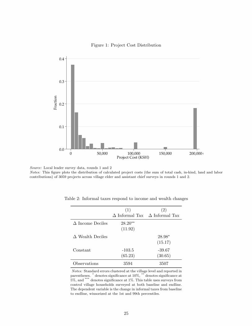
Figure 1: Project Cost Distribution

0.0

0.1

0.2

0.3

0.4Fr

actio

n

0 50,000 100,000 150,000 200,000+Project Cost (KSH)

Source: Local leader survey data, rounds 1 and 2Notes: This figure plots the distribution of calculated project costs (the sum of total cash, in-kind, land and laborcontributions) of 3059 projects across village elder and assistant chief surveys in rounds 1 and 2.

Table 2: Informal taxes respond to income and wealth changes

(1) (2)∆ Informal Tax ∆ Informal Tax

∆ Income Deciles 28.20∗∗

(11.92)

∆ Wealth Deciles 28.98∗

(15.17)

Constant -103.5 -39.67(65.23) (30.65)

Observations 3594 3507

Notes: Standard errors clustered at the village level and reported inparentheses. * denotes significance at 10%, ** denotes significance at5%, and *** denotes significance at 1%. This table uses surveys fromcontrol village households surveyed at both baseline and endline.The dependent variable is the change in informal taxes from baselineto endline, winsorized at the 1st and 99th percentiles.

25

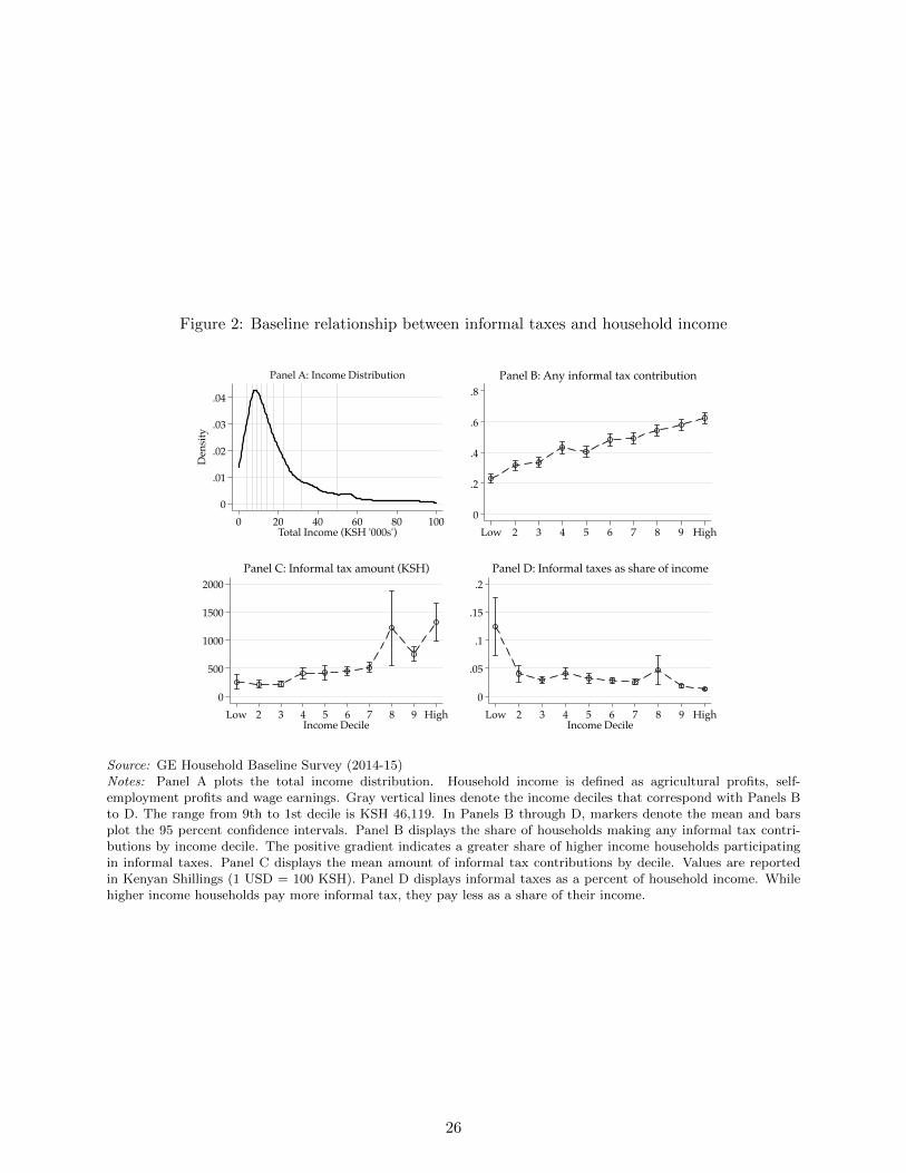
Figure 2: Baseline relationship between informal taxes and household income

0

.01

.02

.03

.04

Den

sity

0 20 40 60 80 100Total Income (KSH '000s')

Panel A: Income Distribution

0

.2

.4

.6

.8

Low 2 3 4 5 6 7 8 9 High

Panel B: Any informal tax contribution

0

500

1000

1500

2000

Low 2 3 4 5 6 7 8 9 HighIncome Decile

Panel C: Informal tax amount (KSH)

0

.05

.1

.15

.2

Low 2 3 4 5 6 7 8 9 HighIncome Decile

Panel D: Informal taxes as share of income

Source: GE Household Baseline Survey (2014-15)Notes: Panel A plots the total income distribution. Household income is defined as agricultural profits, self-employment profits and wage earnings. Gray vertical lines denote the income deciles that correspond with Panels Bto D. The range from 9th to 1st decile is KSH 46,119. In Panels B through D, markers denote the mean and barsplot the 95 percent confidence intervals. Panel B displays the share of households making any informal tax contri-butions by income decile. The positive gradient indicates a greater share of higher income households participatingin informal taxes. Panel C displays the mean amount of informal tax contributions by decile. Values are reportedin Kenyan Shillings (1 USD = 100 KSH). Panel D displays informal taxes as a percent of household income. Whilehigher income households pay more informal tax, they pay less as a share of their income.

26

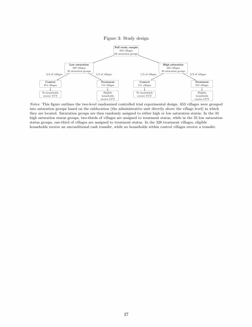
Figure 3: Study design

Full study sample653 villages

68 saturation groups

High saturation324 villages

33 saturation groups

Low saturation329 villages

35 saturation groups

Treatment213 villages

Control111 villages

Treatment115 villages

Control214 villages

Eligiblehouseholds

receive UCT

No householdsreceive UCT

Eligiblehouseholds

receive UCT

No householdsreceive UCT

2/3 of villages1/3 of villages1/3 of villages2/3 of villages

Notes: This figure outlines the two-level randomized controlled trial experimental design. 653 villages were groupedinto saturation groups based on the sublocation (the administrative unit directly above the village level) in whichthey are located. Saturation groups are then randomly assigned to either high or low saturation status. In the 33high saturation status groups, two-thirds of villages are assigned to treatment status, while in the 35 low saturationstatus groups, one-third of villages are assigned to treatment status. In the 328 treatment villages, eligiblehouseholds receive an unconditional cash transfer, while no households within control villages receive a transfer.

27

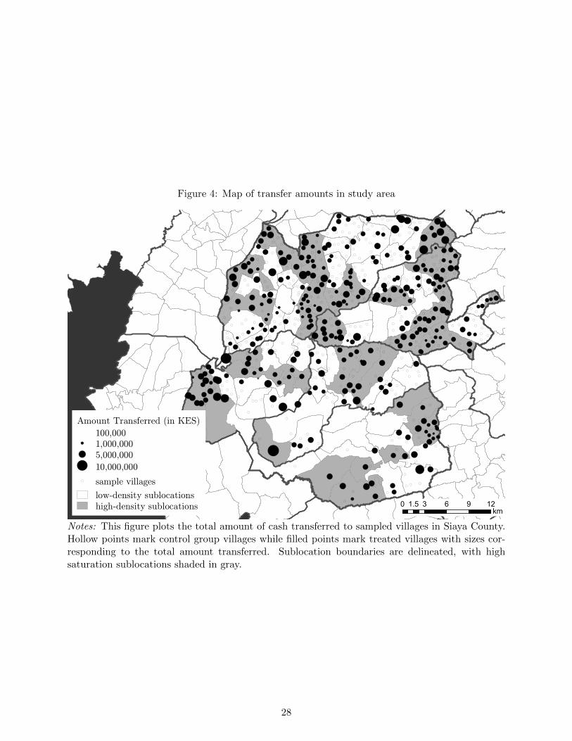
Figure 4: Map of transfer amounts in study area

(

(

(

(

(

(

(

(

( (

(

(

(

(

(( (

(

(

(

(

((

(

(

(

(

(

(

(

((

(

(

((

( (

(

(

(

(

(

(

((

(

(

(

(

(

(

(

(

(

(

((

(

(

((

((

((

(

(

(

((

( (

((

(

(

(

(

(

( (

(

(

((

(

(

((

(

( (

((

(

(

( (

((

(

(

((

((

((

((

(((

((

((

((

(

(

(

( (

(((

((

(

(

((

(

(

(

((

(

(

((

((

(

(

(

((

((

(

(

((

( (

((

(

( ((

(

(

(

(

(

(

((

(

(

(

((

((

((

(

(

(

(

(

(

(

( (

(

(

( (

((

(

((

(

((

(

((

(

((

(

(((

(

(

((

((

(

(

(

(

((

(

((

( (

(( (

(

(

((

(

((

(

(

(

(

((

((

(

(((

((

(

(

(

(

(

((

(

(

(

(

(

( (

(

((

(

(

(

(

(

(

( (

((

(

(

((

(

(

(

(

(

( (

(

((

((

(

(

(

(

(

(

(

(

(

((

(

(

( (

(

(

(

((

(

( (

(

(

(

(

(

(

((

(

(

(

(

(

(

(

(

(

((

(

(

((

((

(

(

((

(

(

(

(

(

(

((

(

(

((

(

(

( (( ( (

(

(

(

(

(

((

((

(

(

((((

(

((

( (

(

(

(

(

(

(

( ((

((

((

(

(

(

(

(

(((

(

(

(

(

( ((

(

(

(

(

(

(

(

(

(

( (( (

((

((

(((

(

((( (

((

(

(

(

((

( (( ( (

(

(

((

(

(

(

( ((

(

(

(

(

((

((

(

(

(((

(

(

(

(

( (

(

(

(

(

(

(

( ( ((

(((

( (

(

((

(

((

(

(

(

(

((

(

(

((

( ( (

((

(

( ( ( ((

(

((

(( (

(

((

(((

( (

(

(

(

((

( (

(( (

((

(

(((

(

((

(

(

( (

(

(( (

(

(

(

( (

((

((

((

(

((

(

(

( (

((

(

((

(

((

( (

((

(

(

( ((

((

(

(

(

(

((

(

((

(

( ((

(

((

((

(

(((

(

(

(

(( (

(

((

((

(

(

(((

((

(

( (

(

((

(

(

(

(

(

(

Amount Transferred (in KES)100,0001,000,0005,000,00010,000,000

( sample villageslow-density sublocationshigh-density sublocations 0 3 6 9 121.5 km

Notes: This figure plots the total amount of cash transferred to sampled villages in Siaya County.Hollow points mark control group villages while filled points mark treated villages with sizes cor-responding to the total amount transferred. Sublocation boundaries are delineated, with highsaturation sublocations shaded in gray.

28

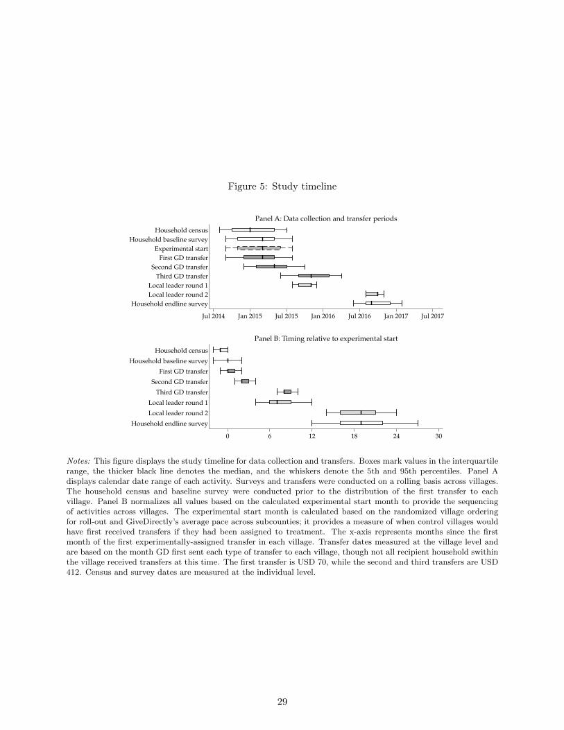
Figure 5: Study timeline

Household censusHousehold baseline survey

Experimental startFirst GD transfer

Second GD transferThird GD transfer

Local leader round 1Local leader round 2

Household endline survey

Jul 2014 Jan 2015 Jul 2015 Jan 2016 Jul 2016 Jan 2017 Jul 2017

Panel A: Data collection and transfer periods

Household censusHousehold baseline survey

First GD transferSecond GD transfer

Third GD transferLocal leader round 1Local leader round 2

Household endline survey

0 6 12 18 24 30

Panel B: Timing relative to experimental start

Notes: This figure displays the study timeline for data collection and transfers. Boxes mark values in the interquartilerange, the thicker black line denotes the median, and the whiskers denote the 5th and 95th percentiles. Panel Adisplays calendar date range of each activity. Surveys and transfers were conducted on a rolling basis across villages.The household census and baseline survey were conducted prior to the distribution of the first transfer to eachvillage. Panel B normalizes all values based on the calculated experimental start month to provide the sequencingof activities across villages. The experimental start month is calculated based on the randomized village orderingfor roll-out and GiveDirectly’s average pace across subcounties; it provides a measure of when control villages wouldhave first received transfers if they had been assigned to treatment. The x-axis represents months since the firstmonth of the first experimentally-assigned transfer in each village. Transfer dates measured at the village level andare based on the month GD first sent each type of transfer to each village, though not all recipient household swithinthe village received transfers at this time. The first transfer is USD 70, while the second and third transfers are USD412. Census and survey dates are measured at the individual level.

29

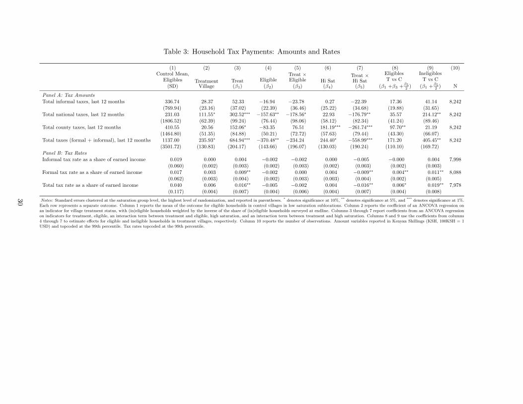
Table 3: Household Tax Payments: Amounts and Rates

(1) (2) (3) (4) (5) (6) (7) (8) (9) (10)Control Mean,

Eligibles(SD)

TreatmentVillage

Treat(β1)

Eligible(β2)

Treat ×Eligible

(β3)Hi Sat(β4)

Treat ×Hi Sat(β5)

EligiblesT vs C

(β1 +β3 +β52 )

IneligiblesT vs C

(β1 +β52 ) N

Panel A: Tax AmountsTotal informal taxes, last 12 months 336.74 28.37 52.33 −16.94 −23.78 0.27 −22.39 17.36 41.14 8,242

(769.94) (23.16) (37.02) (22.39) (36.46) (25.22) (34.68) (19.88) (31.65)Total national taxes, last 12 months 231.03 111.55∗ 302.52∗∗∗ −157.63∗∗ −178.56∗ 22.93 −176.79∗∗ 35.57 214.12∗∗ 8,242

(1806.52) (62.39) (99.24) (76.44) (98.06) (58.12) (82.34) (41.24) (89.46)Total county taxes, last 12 months 410.55 20.56 152.06∗ −83.35 76.51 181.19∗∗∗ −261.74∗∗∗ 97.70∗∗ 21.19 8,242

(1464.80) (51.35) (84.88) (50.21) (72.72) (57.63) (79.44) (43.30) (66.07)Total taxes (formal + informal), last 12 months 1137.00 235.93∗ 684.94∗∗∗ −370.48∗∗ −234.24 244.40∗ −558.99∗∗∗ 171.20 405.45∗∗ 8,242

(3501.72) (130.83) (204.17) (143.66) (196.07) (130.03) (190.24) (110.10) (169.72)Panel B: Tax RatesInformal tax rate as a share of earned income 0.019 0.000 0.004 −0.002 −0.002 0.000 −0.005 −0.000 0.004 7,998

(0.060) (0.002) (0.003) (0.002) (0.003) (0.002) (0.003) (0.002) (0.003)Formal tax rate as a share of earned income 0.017 0.003 0.009∗∗ −0.002 0.000 0.004 −0.009∗∗ 0.004∗∗ 0.011∗∗ 8,088

(0.062) (0.003) (0.004) (0.002) (0.003) (0.003) (0.004) (0.002) (0.005)Total tax rate as a share of earned income 0.040 0.006 0.016∗∗ −0.005 −0.002 0.004 −0.016∗∗ 0.006∗ 0.019∗∗ 7,978

(0.117) (0.004) (0.007) (0.004) (0.006) (0.004) (0.007) (0.004) (0.008)

Notes: Standard errors clustered at the saturation group level, the highest level of randomization, and reported in parentheses. * denotes significance at 10%, ** denotes significance at 5%, and *** denotes significance at 1%.Each row represents a separate outcome. Column 1 reports the mean of the outcome for eligible households in control villages in low saturation sublocations. Column 2 reports the coefficient of an ANCOVA regression onan indicator for village treatment status, with (in)eligible households weighted by the inverse of the share of (in)eligible households surveyed at endline. Columns 3 through 7 report coefficients from an ANCOVA regressionon indicators for treatment, eligible, an interaction term between treatment and eligible, high saturation, and an interaction term between treatment and high saturation. Columns 8 and 9 use the coefficients from columns4 through 7 to estimate effects for eligible and ineligible households in treatment villages, respectively. Column 10 reports the number of observations. Amount variables reported in Kenyan Shillings (KSH, 100KSH = 1USD) and topcoded at the 99th percentile. Tax rates topcoded at the 99th percentile.

30

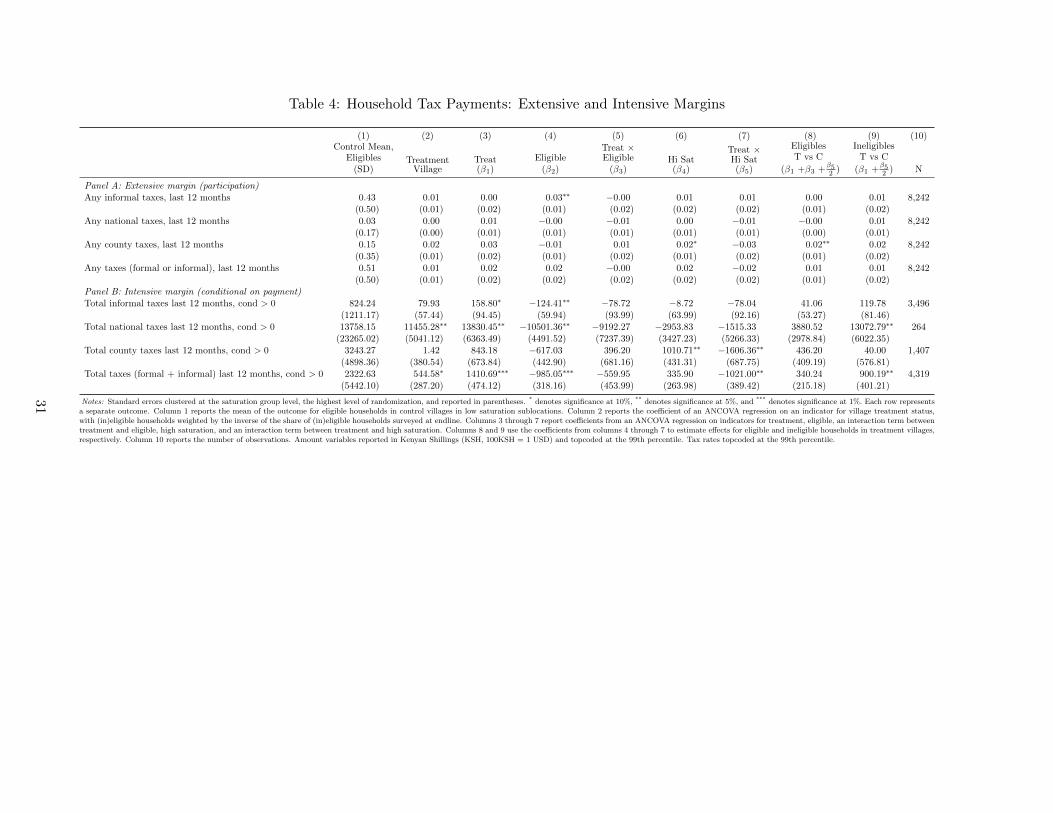
Table 4: Household Tax Payments: Extensive and Intensive Margins

(1) (2) (3) (4) (5) (6) (7) (8) (9) (10)Control Mean,

Eligibles(SD)

TreatmentVillage

Treat(β1)

Eligible(β2)

Treat ×Eligible

(β3)Hi Sat(β4)

Treat ×Hi Sat(β5)

EligiblesT vs C

(β1 +β3 +β52 )

IneligiblesT vs C

(β1 +β52 ) N

Panel A: Extensive margin (participation)Any informal taxes, last 12 months 0.43 0.01 0.00 0.03∗∗ −0.00 0.01 0.01 0.00 0.01 8,242

(0.50) (0.01) (0.02) (0.01) (0.02) (0.02) (0.02) (0.01) (0.02)Any national taxes, last 12 months 0.03 0.00 0.01 −0.00 −0.01 0.00 −0.01 −0.00 0.01 8,242

(0.17) (0.00) (0.01) (0.01) (0.01) (0.01) (0.01) (0.00) (0.01)Any county taxes, last 12 months 0.15 0.02 0.03 −0.01 0.01 0.02∗ −0.03 0.02∗∗ 0.02 8,242

(0.35) (0.01) (0.02) (0.01) (0.02) (0.01) (0.02) (0.01) (0.02)Any taxes (formal or informal), last 12 months 0.51 0.01 0.02 0.02 −0.00 0.02 −0.02 0.01 0.01 8,242

(0.50) (0.01) (0.02) (0.02) (0.02) (0.02) (0.02) (0.01) (0.02)Panel B: Intensive margin (conditional on payment)Total informal taxes last 12 months, cond > 0 824.24 79.93 158.80∗ −124.41∗∗ −78.72 −8.72 −78.04 41.06 119.78 3,496

(1211.17) (57.44) (94.45) (59.94) (93.99) (63.99) (92.16) (53.27) (81.46)Total national taxes last 12 months, cond > 0 13758.15 11455.28∗∗ 13830.45∗∗ −10501.36∗∗ −9192.27 −2953.83 −1515.33 3880.52 13072.79∗∗ 264

(23265.02) (5041.12) (6363.49) (4491.52) (7237.39) (3427.23) (5266.33) (2978.84) (6022.35)Total county taxes last 12 months, cond > 0 3243.27 1.42 843.18 −617.03 396.20 1010.71∗∗ −1606.36∗∗ 436.20 40.00 1,407

(4898.36) (380.54) (673.84) (442.90) (681.16) (431.31) (687.75) (409.19) (576.81)Total taxes (formal + informal) last 12 months, cond > 0 2322.63 544.58∗ 1410.69∗∗∗ −985.05∗∗∗ −559.95 335.90 −1021.00∗∗ 340.24 900.19∗∗ 4,319

(5442.10) (287.20) (474.12) (318.16) (453.99) (263.98) (389.42) (215.18) (401.21)

Notes: Standard errors clustered at the saturation group level, the highest level of randomization, and reported in parentheses. * denotes significance at 10%, ** denotes significance at 5%, and *** denotes significance at 1%. Each row representsa separate outcome. Column 1 reports the mean of the outcome for eligible households in control villages in low saturation sublocations. Column 2 reports the coefficient of an ANCOVA regression on an indicator for village treatment status,with (in)eligible households weighted by the inverse of the share of (in)eligible households surveyed at endline. Columns 3 through 7 report coefficients from an ANCOVA regression on indicators for treatment, eligible, an interaction term betweentreatment and eligible, high saturation, and an interaction term between treatment and high saturation. Columns 8 and 9 use the coefficients from columns 4 through 7 to estimate effects for eligible and ineligible households in treatment villages,respectively. Column 10 reports the number of observations. Amount variables reported in Kenyan Shillings (KSH, 100KSH = 1 USD) and topcoded at the 99th percentile. Tax rates topcoded at the 99th percentile.

31

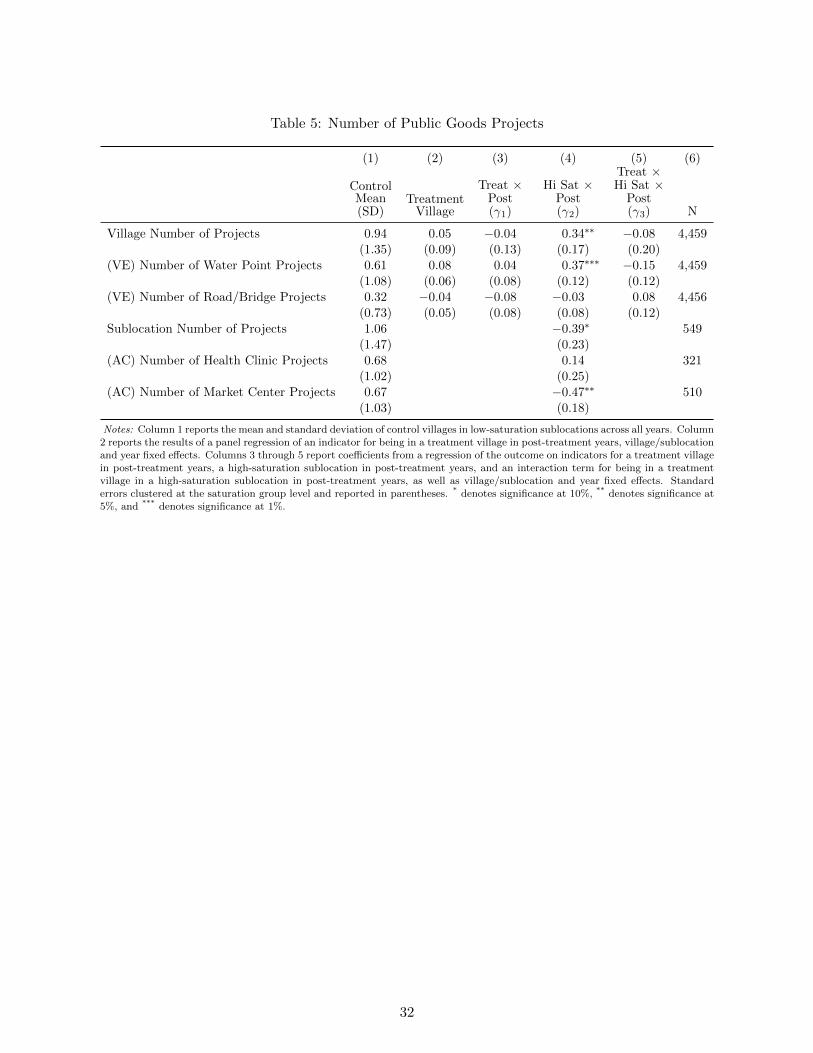
Table 5: Number of Public Goods Projects

(1) (2) (3) (4) (5) (6)

ControlMean(SD)

TreatmentVillage

Treat ×Post(γ1)

Hi Sat ×Post(γ2)

Treat ×Hi Sat ×

Post(γ3) N

Village Number of Projects 0.94 0.05 −0.04 0.34∗∗ −0.08 4,459(1.35) (0.09) (0.13) (0.17) (0.20)

(VE) Number of Water Point Projects 0.61 0.08 0.04 0.37∗∗∗ −0.15 4,459(1.08) (0.06) (0.08) (0.12) (0.12)

(VE) Number of Road/Bridge Projects 0.32 −0.04 −0.08 −0.03 0.08 4,456(0.73) (0.05) (0.08) (0.08) (0.12)

Sublocation Number of Projects 1.06 −0.39∗ 549(1.47) (0.23)

(AC) Number of Health Clinic Projects 0.68 0.14 321(1.02) (0.25)

(AC) Number of Market Center Projects 0.67 −0.47∗∗ 510(1.03) (0.18)

Notes: Column 1 reports the mean and standard deviation of control villages in low-saturation sublocations across all years. Column2 reports the results of a panel regression of an indicator for being in a treatment village in post-treatment years, village/sublocationand year fixed effects. Columns 3 through 5 report coefficients from a regression of the outcome on indicators for a treatment villagein post-treatment years, a high-saturation sublocation in post-treatment years, and an interaction term for being in a treatmentvillage in a high-saturation sublocation in post-treatment years, as well as village/sublocation and year fixed effects. Standarderrors clustered at the saturation group level and reported in parentheses. * denotes significance at 10%, ** denotes significance at5%, and *** denotes significance at 1%.

32

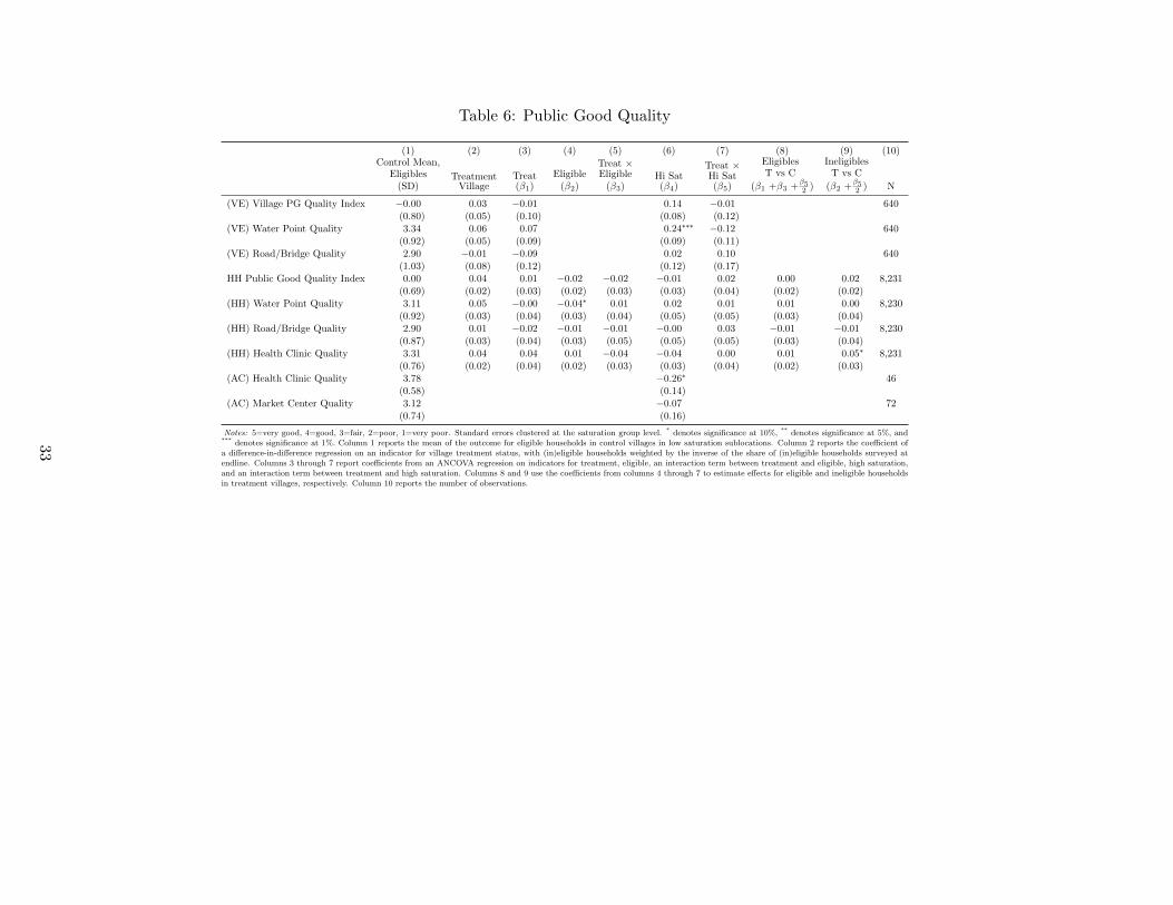
Table 6: Public Good Quality

(1) (2) (3) (4) (5) (6) (7) (8) (9) (10)Control Mean,

Eligibles(SD)

TreatmentVillage

Treat(β1)

Eligible(β2)

Treat ×Eligible

(β3)Hi Sat(β4)

Treat ×Hi Sat(β5)

EligiblesT vs C

(β1 +β3 +β52 )

IneligiblesT vs C

(β2 +β52 ) N

(VE) Village PG Quality Index −0.00 0.03 −0.01 0.14 −0.01 640(0.80) (0.05) (0.10) (0.08) (0.12)

(VE) Water Point Quality 3.34 0.06 0.07 0.24∗∗∗ −0.12 640(0.92) (0.05) (0.09) (0.09) (0.11)

(VE) Road/Bridge Quality 2.90 −0.01 −0.09 0.02 0.10 640(1.03) (0.08) (0.12) (0.12) (0.17)

HH Public Good Quality Index 0.00 0.04 0.01 −0.02 −0.02 −0.01 0.02 0.00 0.02 8,231(0.69) (0.02) (0.03) (0.02) (0.03) (0.03) (0.04) (0.02) (0.02)

(HH) Water Point Quality 3.11 0.05 −0.00 −0.04∗ 0.01 0.02 0.01 0.01 0.00 8,230(0.92) (0.03) (0.04) (0.03) (0.04) (0.05) (0.05) (0.03) (0.04)

(HH) Road/Bridge Quality 2.90 0.01 −0.02 −0.01 −0.01 −0.00 0.03 −0.01 −0.01 8,230(0.87) (0.03) (0.04) (0.03) (0.05) (0.05) (0.05) (0.03) (0.04)

(HH) Health Clinic Quality 3.31 0.04 0.04 0.01 −0.04 −0.04 0.00 0.01 0.05∗ 8,231(0.76) (0.02) (0.04) (0.02) (0.03) (0.03) (0.04) (0.02) (0.03)

(AC) Health Clinic Quality 3.78 −0.26∗ 46(0.58) (0.14)

(AC) Market Center Quality 3.12 −0.07 72(0.74) (0.16)

Notes: 5=very good, 4=good, 3=fair, 2=poor, 1=very poor. Standard errors clustered at the saturation group level. * denotes significance at 10%, ** denotes significance at 5%, and*** denotes significance at 1%. Column 1 reports the mean of the outcome for eligible households in control villages in low saturation sublocations. Column 2 reports the coefficient ofa difference-in-difference regression on an indicator for village treatment status, with (in)eligible households weighted by the inverse of the share of (in)eligible households surveyed atendline. Columns 3 through 7 report coefficients from an ANCOVA regression on indicators for treatment, eligible, an interaction term between treatment and eligible, high saturation,and an interaction term between treatment and high saturation. Columns 8 and 9 use the coefficients from columns 4 through 7 to estimate effects for eligible and ineligible householdsin treatment villages, respectively. Column 10 reports the number of observations.

33

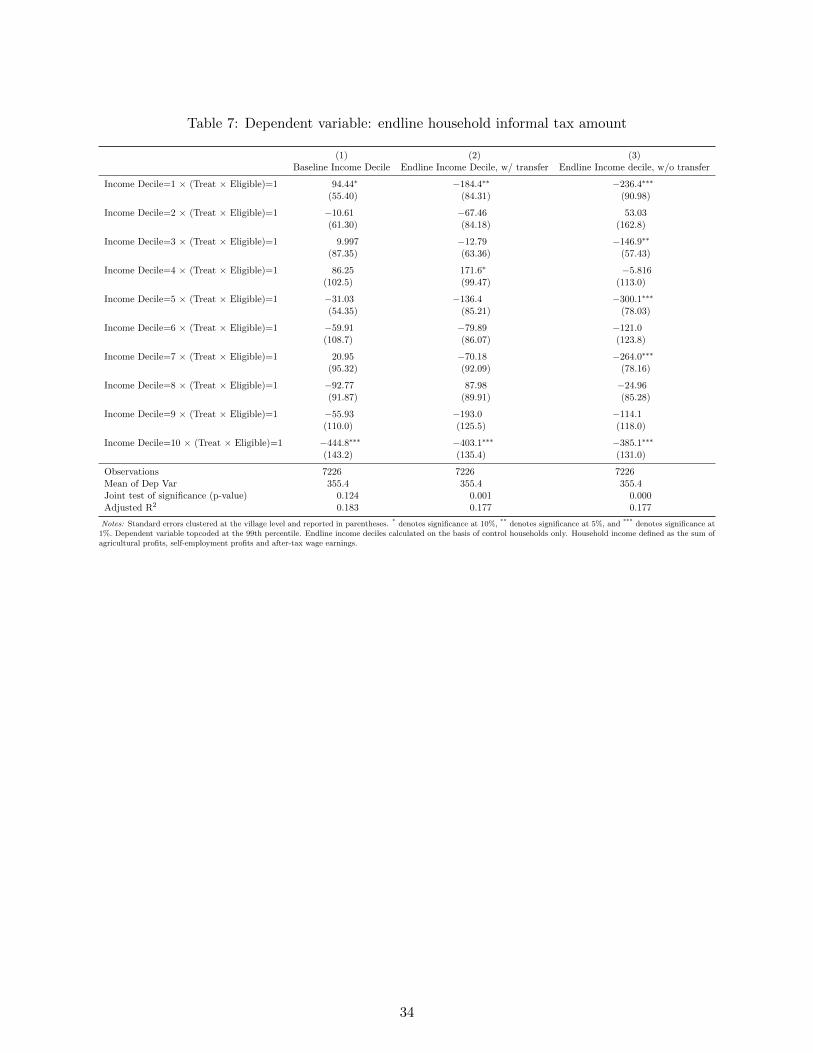
Table 7: Dependent variable: endline household informal tax amount

(1) (2) (3)Baseline Income Decile Endline Income Decile, w/ transfer Endline Income decile, w/o transfer

Income Decile=1 × (Treat × Eligible)=1 94.44∗ −184.4∗∗ −236.4∗∗∗

(55.40) (84.31) (90.98)

Income Decile=2 × (Treat × Eligible)=1 −10.61 −67.46 53.03(61.30) (84.18) (162.8)

Income Decile=3 × (Treat × Eligible)=1 9.997 −12.79 −146.9∗∗

(87.35) (63.36) (57.43)

Income Decile=4 × (Treat × Eligible)=1 86.25 171.6∗ −5.816(102.5) (99.47) (113.0)

Income Decile=5 × (Treat × Eligible)=1 −31.03 −136.4 −300.1∗∗∗

(54.35) (85.21) (78.03)

Income Decile=6 × (Treat × Eligible)=1 −59.91 −79.89 −121.0(108.7) (86.07) (123.8)

Income Decile=7 × (Treat × Eligible)=1 20.95 −70.18 −264.0∗∗∗

(95.32) (92.09) (78.16)

Income Decile=8 × (Treat × Eligible)=1 −92.77 87.98 −24.96(91.87) (89.91) (85.28)

Income Decile=9 × (Treat × Eligible)=1 −55.93 −193.0 −114.1(110.0) (125.5) (118.0)

Income Decile=10 × (Treat × Eligible)=1 −444.8∗∗∗ −403.1∗∗∗ −385.1∗∗∗

(143.2) (135.4) (131.0)

Observations 7226 7226 7226Mean of Dep Var 355.4 355.4 355.4Joint test of significance (p-value) 0.124 0.001 0.000Adjusted R2 0.183 0.177 0.177

Notes: Standard errors clustered at the village level and reported in parentheses. * denotes significance at 10%, ** denotes significance at 5%, and *** denotes significance at1%. Dependent variable topcoded at the 99th percentile. Endline income deciles calculated on the basis of control households only. Household income defined as the sum ofagricultural profits, self-employment profits and after-tax wage earnings.

34

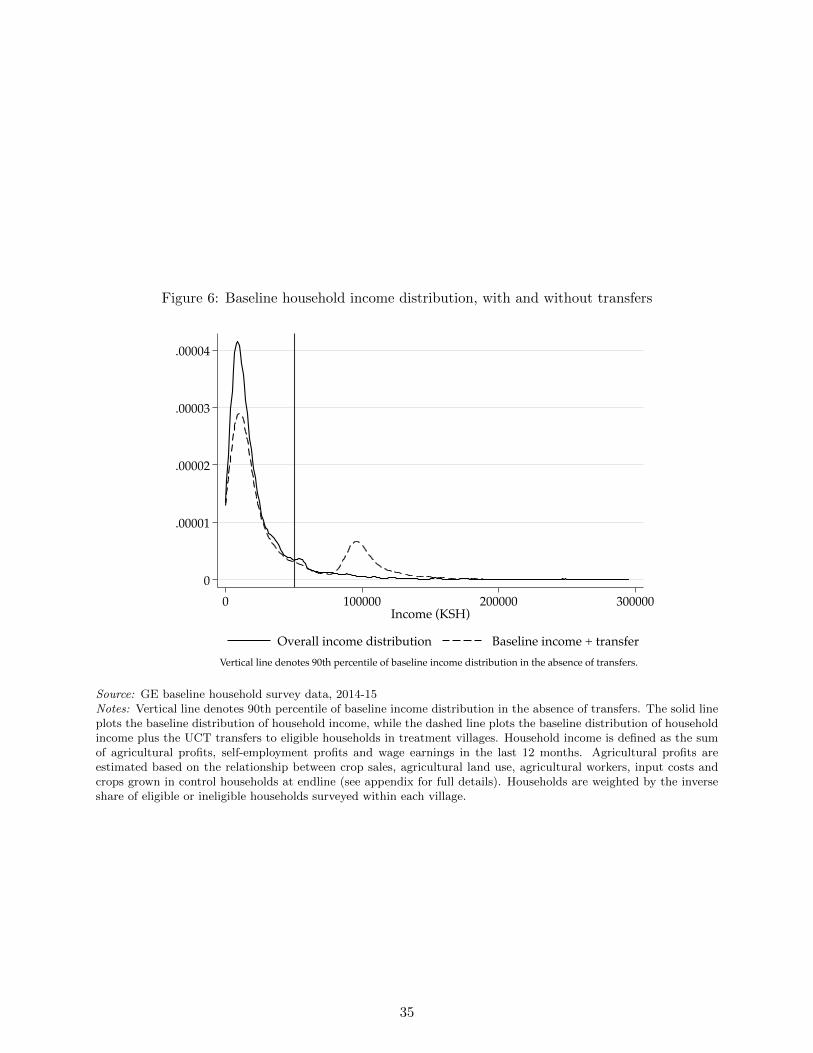
Figure 6: Baseline household income distribution, with and without transfers

0

.00001

.00002

.00003

.00004

0 100000 200000 300000Income (KSH)

Overall income distribution Baseline income + transferVertical line denotes 90th percentile of baseline income distribution in the absence of transfers.

Source: GE baseline household survey data, 2014-15Notes: Vertical line denotes 90th percentile of baseline income distribution in the absence of transfers. The solid lineplots the baseline distribution of household income, while the dashed line plots the baseline distribution of householdincome plus the UCT transfers to eligible households in treatment villages. Household income is defined as the sumof agricultural profits, self-employment profits and wage earnings in the last 12 months. Agricultural profits areestimated based on the relationship between crop sales, agricultural land use, agricultural workers, input costs andcrops grown in control households at endline (see appendix for full details). Households are weighted by the inverseshare of eligible or ineligible households surveyed within each village.

35

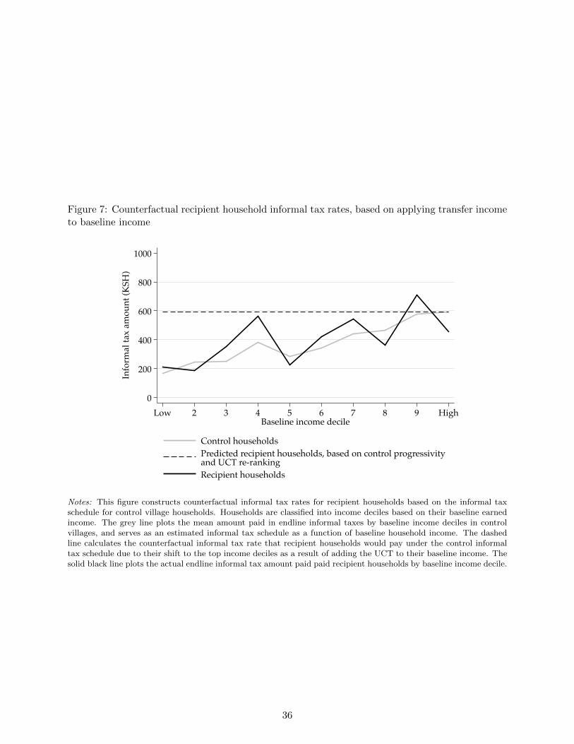
Figure 7: Counterfactual recipient household informal tax rates, based on applying transfer incometo baseline income

0

200

400

600

800

1000

Info

rmal

tax

amou

nt (K

SH)

Low 2 3 4 5 6 7 8 9 HighBaseline income decile

Control householdsPredicted recipient households, based on control progressivityand UCT re-rankingRecipient households

Notes: This figure constructs counterfactual informal tax rates for recipient households based on the informal taxschedule for control village households. Households are classified into income deciles based on their baseline earnedincome. The grey line plots the mean amount paid in endline informal taxes by baseline income deciles in controlvillages, and serves as an estimated informal tax schedule as a function of baseline household income. The dashedline calculates the counterfactual informal tax rate that recipient households would pay under the control informaltax schedule due to their shift to the top income deciles as a result of adding the UCT to their baseline income. Thesolid black line plots the actual endline informal tax amount paid paid recipient households by baseline income decile.

36

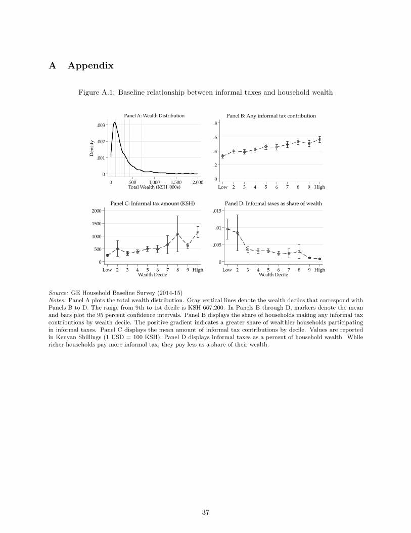
A Appendix

Figure A.1: Baseline relationship between informal taxes and household wealth

0

.001

.002

.003

Den

sity

0 500 1,000 1,500 2,000Total Wealth (KSH '000s)

Panel A: Wealth Distribution

0

.2

.4

.6

.8

Low 2 3 4 5 6 7 8 9 High

Panel B: Any informal tax contribution

0

500

1000

1500

2000

Low 2 3 4 5 6 7 8 9 HighWealth Decile

Panel C: Informal tax amount (KSH)

0

.005

.01

.015

Low 2 3 4 5 6 7 8 9 HighWealth Decile

Panel D: Informal taxes as share of wealth

Source: GE Household Baseline Survey (2014-15)Notes: Panel A plots the total wealth distribution. Gray vertical lines denote the wealth deciles that correspond withPanels B to D. The range from 9th to 1st decile is KSH 667,200. In Panels B through D, markers denote the meanand bars plot the 95 percent confidence intervals. Panel B displays the share of households making any informal taxcontributions by wealth decile. The positive gradient indicates a greater share of wealthier households participatingin informal taxes. Panel C displays the mean amount of informal tax contributions by decile. Values are reportedin Kenyan Shillings (1 USD = 100 KSH). Panel D displays informal taxes as a percent of household wealth. Whilericher households pay more informal tax, they pay less as a share of their wealth.

37

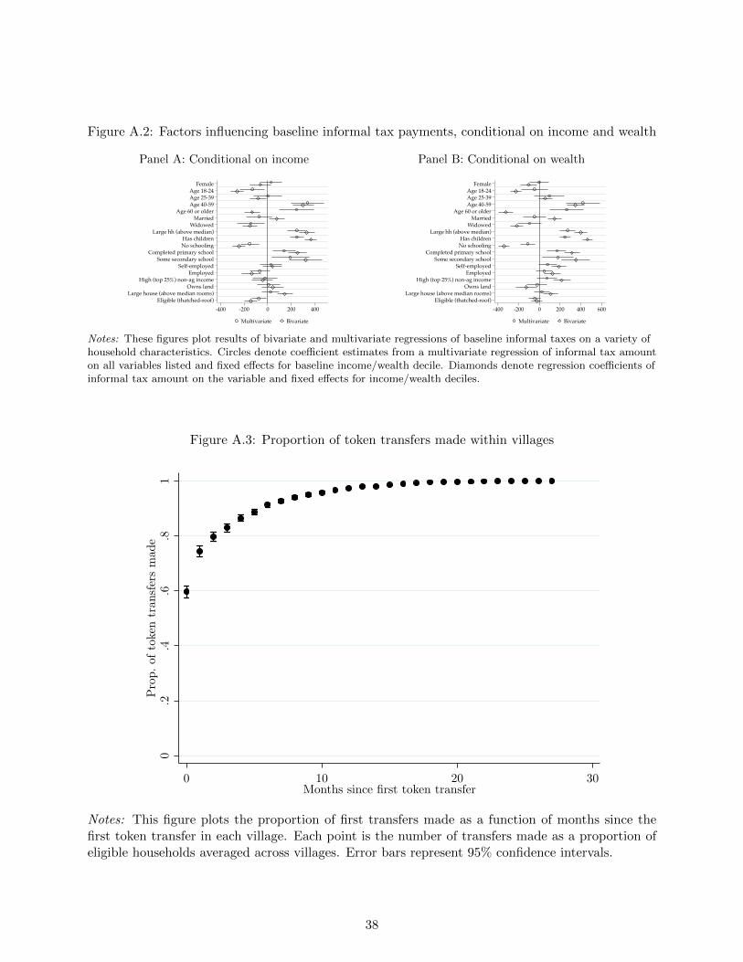
Figure A.2: Factors influencing baseline informal tax payments, conditional on income and wealth

Panel A: Conditional on income

FemaleAge 18-24Age 25-39Age 40-59

Age 60 or olderMarried

WidowedLarge hh (above median)

Has childrenNo schooling

Completed primary schoolSome secondary school

Self-employedEmployed

High (top 25%) non-ag incomeOwns land

Large house (above median rooms)Eligible (thatched-roof)

-400 -200 0 200 400

Multivariate Bivariate

Panel B: Conditional on wealth

FemaleAge 18-24Age 25-39Age 40-59

Age 60 or olderMarried

WidowedLarge hh (above median)

Has childrenNo schooling

Completed primary schoolSome secondary school

Self-employedEmployed

High (top 25%) non-ag incomeOwns land

Large house (above median rooms)Eligible (thatched-roof)

-400 -200 0 200 400 600

Multivariate Bivariate

Notes: These figures plot results of bivariate and multivariate regressions of baseline informal taxes on a variety ofhousehold characteristics. Circles denote coefficient estimates from a multivariate regression of informal tax amounton all variables listed and fixed effects for baseline income/wealth decile. Diamonds denote regression coefficients ofinformal tax amount on the variable and fixed effects for income/wealth deciles.

Figure A.3: Proportion of token transfers made within villages

0.2

.4.6

.81

Prop

. of t

oken

tran

sfers

mad

e

0 10 20 30Months since first token transfer

Notes: This figure plots the proportion of first transfers made as a function of months since thefirst token transfer in each village. Each point is the number of transfers made as a proportion ofeligible households averaged across villages. Error bars represent 95% confidence intervals.

38

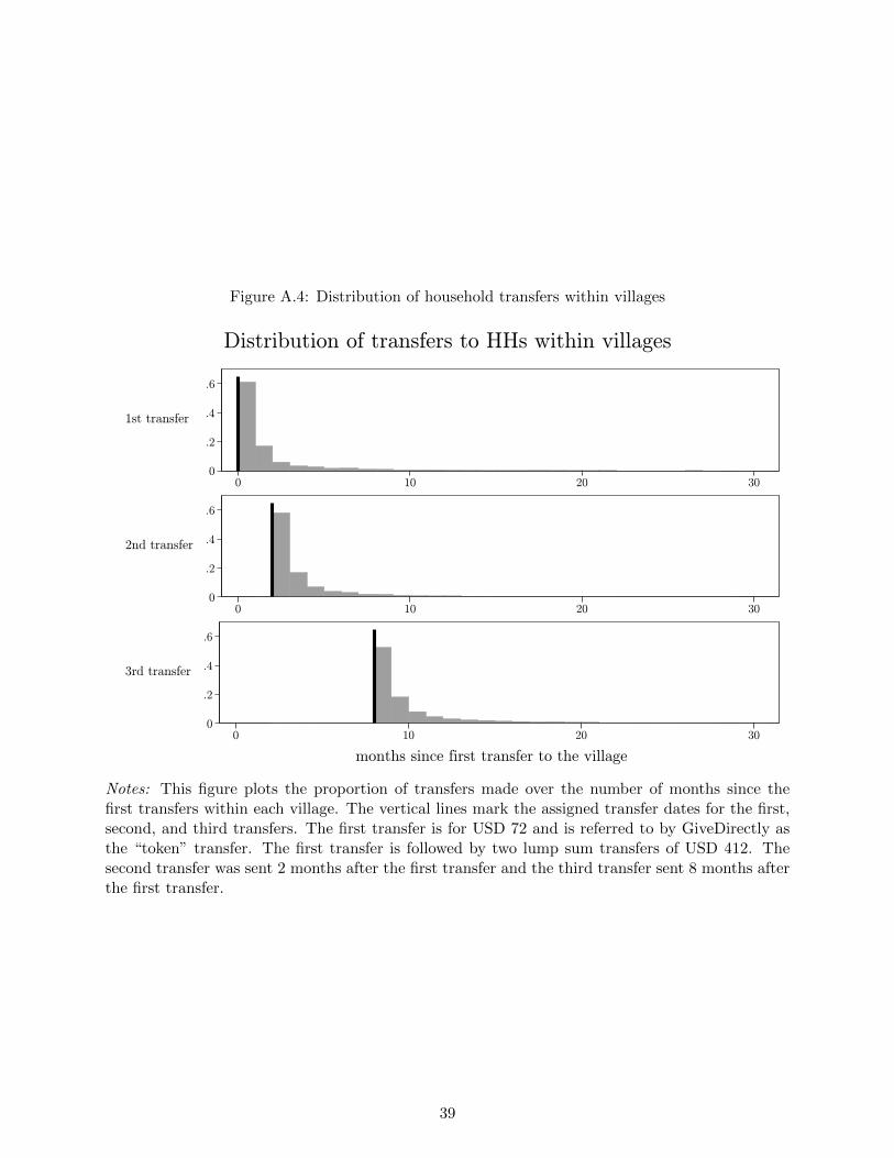
Figure A.4: Distribution of household transfers within villages

0

.2

.4

.6

1st transfer

0 10 20 30

0

.2

.4

.6

2nd transfer

0 10 20 30

0

.2

.4

.6

3rd transfer

0 10 20 30

months since first transfer to the village

Distribution of transfers to HHs within villages

Notes: This figure plots the proportion of transfers made over the number of months since thefirst transfers within each village. The vertical lines mark the assigned transfer dates for the first,second, and third transfers. The first transfer is for USD 72 and is referred to by GiveDirectly asthe “token” transfer. The first transfer is followed by two lump sum transfers of USD 412. Thesecond transfer was sent 2 months after the first transfer and the third transfer sent 8 months afterthe first transfer.

39

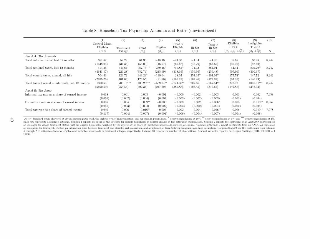
Table 8: Household Tax Payments: Amounts and Rates (unwinsorized)

(1) (2) (3) (4) (5) (6) (7) (8) (9) (10)Control Mean,

Eligibles(SD)

TreatmentVillage

Treat(β1)

Eligible(β2)

Treat ×Eligible

(β3)Hi Sat(β4)

Treat ×Hi Sat(β5)

EligiblesT vs C

(β1 +β3 +β52 )

IneligiblesT vs C

(β1 +β52 ) N

Panel A: Tax AmountsTotal informal taxes, last 12 months 381.87 52.29 61.36 −48.16 −41.80 −1.14 −1.76 18.68 60.48 8,242

(1348.05) (34.36) (55.00) (46.57) (66.67) (46.79) (63.65) (40.26) (52.60)Total national taxes, last 12 months 414.36 544.64∗∗ 987.76∗∗∗ −389.16∗ −750.85∗∗ −71.33 −364.94 54.44 805.29∗∗ 8,242

(4641.17) (229.28) (352.74) (215.99) (338.19) (156.95) (259.48) (97.96) (310.67)Total county taxes, annual, all hhs 504.43 123.72 343.24∗ −139.04 28.02 251.35∗∗ −391.03∗∗ 175.74∗ 147.72 8,242

(2995.76) (101.03) (176.55) (91.86) (160.25) (102.46) (172.99) (93.85) (146.93)Total taxes (formal + informal), last 12 months 1300.65 705.13∗∗∗ 1400.28∗∗∗ −539.04∗∗ −774.08∗∗ 207.66 −767.54∗∗ 242.42 1016.51∗∗∗ 8,242

(5690.50) (255.55) (402.34) (247.29) (385.88) (193.45) (319.62) (149.88) (342.03)Panel B: Tax RatesInformal tax rate as a share of earned income 0.018 0.001 0.003 −0.002 −0.000 −0.002 −0.003 0.001 0.002 7,958

(0.061) (0.002) (0.004) (0.002) (0.003) (0.002) (0.003) (0.002) (0.004)Formal tax rate as a share of earned income 0.016 0.004 0.009∗∗ −0.000 −0.003 0.002 −0.006∗ 0.003 0.010∗∗ 8,052

(0.067) (0.003) (0.004) (0.002) (0.003) (0.002) (0.004) (0.002) (0.004)Total tax rate as a share of earned income 0.040 0.006 0.016∗∗ −0.005 −0.002 0.004 −0.016∗∗ 0.006∗ 0.019∗∗ 7,978

(0.117) (0.004) (0.007) (0.004) (0.006) (0.004) (0.007) (0.004) (0.008)

Notes: Standard errors clustered at the saturation group level, the highest level of randomization, and reported in parentheses. * denotes significance at 10%, ** denotes significance at 5%, and *** denotes significance at 1%.Each row represents a separate outcome. Column 1 reports the mean of the outcome for eligible households in control villages in low saturation sublocations. Column 2 reports the coefficient of an ANCOVA regression onan indicator for village treatment status, with (in)eligible households weighted by the inverse of the share of (in)eligible households surveyed at endline. Columns 3 through 7 report coefficients from an ANCOVA regressionon indicators for treatment, eligible, an interaction term between treatment and eligible, high saturation, and an interaction term between treatment and high saturation. Columns 8 and 9 use the coefficients from columns4 through 7 to estimate effects for eligible and ineligible households in treatment villages, respectively. Column 10 reports the number of observations. Amount variables reported in Kenyan Shillings (KSH, 100KSH = 1USD).

40

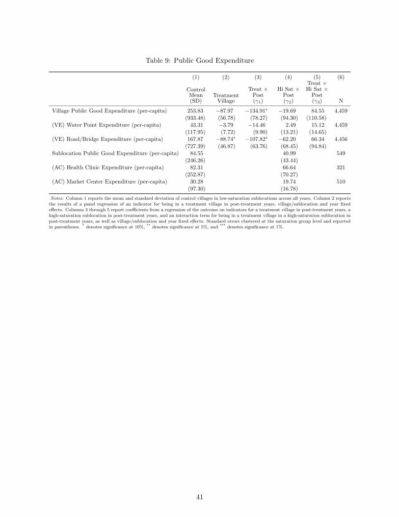
Table 9: Public Good Expenditure

(1) (2) (3) (4) (5) (6)

ControlMean(SD)

TreatmentVillage

Treat ×Post(γ1)

Hi Sat ×Post(γ2)

Treat ×Hi Sat ×

Post(γ3) N

Village Public Good Expenditure (per-capita) 253.83 −87.97 −134.91∗ −19.69 84.55 4,459(933.48) (56.78) (78.27) (94.30) (110.58)

(VE) Water Point Expenditure (per-capita) 43.31 −3.79 −14.46 2.49 15.12 4,459(117.95) (7.72) (9.90) (13.21) (14.65)

(VE) Road/Bridge Expenditure (per-capita) 167.87 −88.74∗ −107.82∗ −62.20 66.34 4,456(727.39) (46.87) (63.76) (68.45) (94.84)

Sublocation Public Good Expenditure (per-capita) 84.55 40.99 549(246.26) (43.44)

(AC) Health Clinic Expenditure (per-capita) 82.31 66.64 321(252.87) (70.27)

(AC) Market Center Expenditure (per-capita) 30.28 19.74 510(97.30) (16.78)

Notes: Column 1 reports the mean and standard deviation of control villages in low-saturation sublocations across all years. Column 2 reportsthe results of a panel regression of an indicator for being in a treatment village in post-treatment years, village/sublocation and year fixedeffects. Columns 3 through 5 report coefficients from a regression of the outcome on indicators for a treatment village in post-treatment years, ahigh-saturation sublocation in post-treatment years, and an interaction term for being in a treatment village in a high-saturation sublocation inpost-treatment years, as well as village/sublocation and year fixed effects. Standard errors clustered at the saturation group level and reportedin parentheses. * denotes significance at 10%, ** denotes significance at 5%, and *** denotes significance at 1%.

41

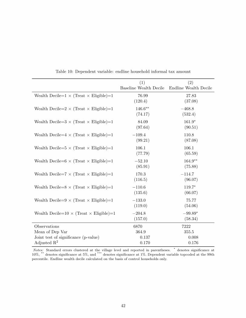
Table 10: Dependent variable: endline household informal tax amount

(1) (2)Baseline Wealth Decile Endline Wealth Decile

Wealth Decile=1 × (Treat × Eligible)=1 76.99 27.83(120.4) (37.08)

Wealth Decile=2 × (Treat × Eligible)=1 146.6∗∗ −468.8(74.17) (532.4)

Wealth Decile=3 × (Treat × Eligible)=1 84.09 161.9∗

(97.64) (90.51)

Wealth Decile=4 × (Treat × Eligible)=1 −109.4 110.8(99.21) (87.08)

Wealth Decile=5 × (Treat × Eligible)=1 106.1 106.1(77.79) (65.59)

Wealth Decile=6 × (Treat × Eligible)=1 −52.10 164.9∗∗

(85.91) (75.88)

Wealth Decile=7 × (Treat × Eligible)=1 170.3 −114.7(116.5) (96.07)

Wealth Decile=8 × (Treat × Eligible)=1 −110.6 119.7∗

(135.6) (66.07)

Wealth Decile=9 × (Treat × Eligible)=1 −133.0 75.77(119.0) (54.06)

Wealth Decile=10 × (Treat × Eligible)=1 −204.8 −99.89∗

(157.0) (58.34)

Observations 6870 7222Mean of Dep Var 364.9 355.5Joint test of significance (p-value) 0.137 0.008Adjusted R2 0.170 0.176

Notes: Standard errors clustered at the village level and reported in parentheses. * denotes significance at10%, ** denotes significance at 5%, and *** denotes significance at 1%. Dependent variable topcoded at the 99thpercentile. Endline wealth decile calculated on the basis of control households only.

42

B Additional details on data collection and intervention

This section contains additional details on the data collection, study context and program inter-

vention by GiveDirectly. Tables 11 and 12 document the high tracking rates achieved by both the

household and local leader surveys across rounds. Table 13 provides details on the range of village

sizes and its implications for the share of households surveyed in each village. Table 14 documents

how Siaya compares to other parts of Kenya, using data from the 2009 Kenya Population and

Housing Census. This census took place prior to devolution and the establishment of the county

system of government; instead, data is aggregated to the district level. The study area is located

entirely within the former Siaya district, and I compare Siaya district with the other districts in

existence at the time of the 2009 census.

Section B.1 outlines the steps in GD’s enrollment process in more detail.

43

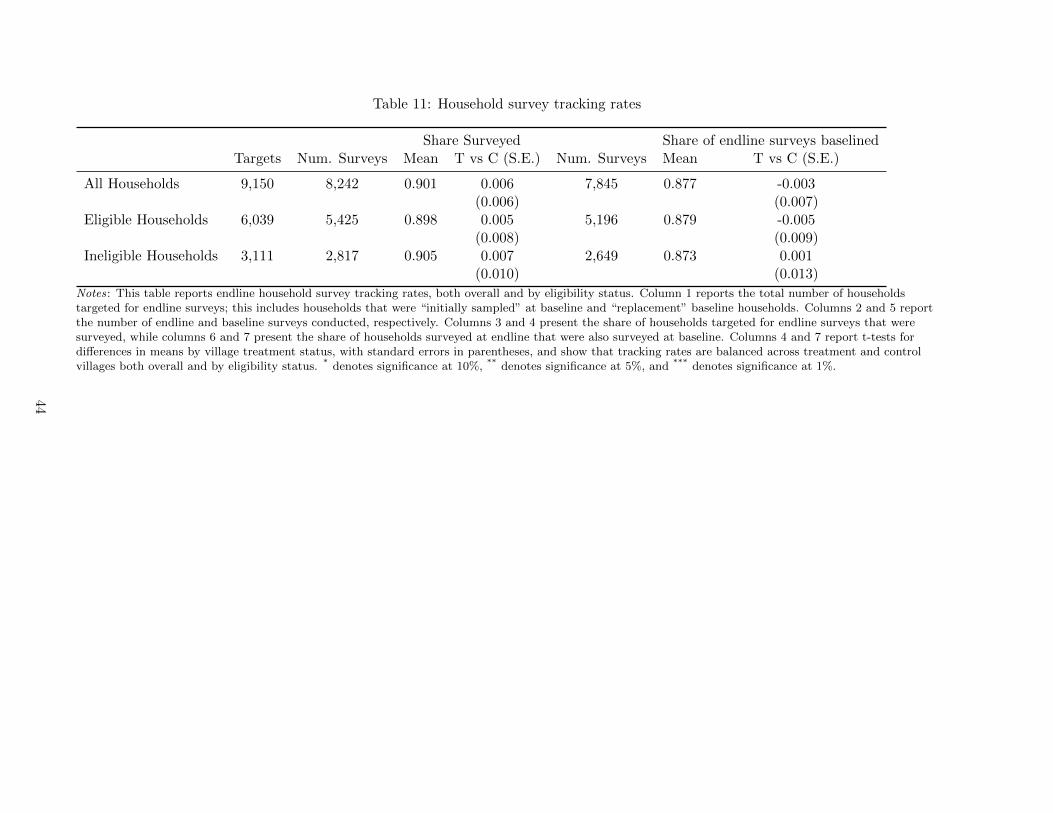
Table 11: Household survey tracking rates

Share Surveyed Share of endline surveys baselinedTargets Num. Surveys Mean T vs C (S.E.) Num. Surveys Mean T vs C (S.E.)

All Households 9,150 8,242 0.901 0.006 7,845 0.877 -0.003(0.006) (0.007)

Eligible Households 6,039 5,425 0.898 0.005 5,196 0.879 -0.005(0.008) (0.009)

Ineligible Households 3,111 2,817 0.905 0.007 2,649 0.873 0.001(0.010) (0.013)

Notes: This table reports endline household survey tracking rates, both overall and by eligibility status. Column 1 reports the total number of householdstargeted for endline surveys; this includes households that were “initially sampled” at baseline and “replacement” baseline households. Columns 2 and 5 reportthe number of endline and baseline surveys conducted, respectively. Columns 3 and 4 present the share of households targeted for endline surveys that weresurveyed, while columns 6 and 7 present the share of households surveyed at endline that were also surveyed at baseline. Columns 4 and 7 report t-tests fordifferences in means by village treatment status, with standard errors in parentheses, and show that tracking rates are balanced across treatment and controlvillages both overall and by eligibility status. * denotes significance at 10%, ** denotes significance at 5%, and *** denotes significance at 1%.

44

Table 12: Local leader tracking rates

Round 1 Round 2Share Surveyed Share Surveyed

Targets Surveyed Mean

T - C /

Hi - Low (SE) Targets Surveyed Mean

T - C /

Hi - Low (SE)

Villages (Village Elders)a 653 633 0.969 0.013 653 640 0.980 -0.021*

(0.013) (0.011)Sublocations (Assistant Chiefs) 84 84 1.000 0.000 84 73 0.869 -0.043

(0.000) (0.075)a: Numbers reported at the GE village level, which corresponds to census enumeration areas. In some cases more than one village elder was surveyed per GEvillage.Notes: This table reports local leader survey tracking rates. Columns 1 through 4 report on the first round of local leader surveys, conducted from July toDecember 2015, while columns 5 through 8 report on the second round, conducted from July to December 2016. Columns 1 and 5 report the total targetnumber of villages and sublocations; this comprises the total number in our study. Columns 2 and 6 report the number of surveys conducted in each round,while columns 3 and 7 report tracking rates by round. Columns 4 and 8 report t-tests for differences in means; at the village level, this tests for differences insurvey rates for treatment versus control villages. At the sublocation level, this tests for differences in high saturation sublocations versus low saturationsublocations. Standard errors are reported in parentheses. * denotes significance at 10%, ** denotes significance at 5%, and *** denotes significance at 1%.45

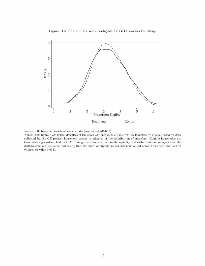
Figure B.5: Share of households eligible for GD transfers by village

0

1

2

3

4D

ensi

ty

0 .1 .2 .3 .4 .5 .6Proportion Eligible

Treatment Control

Source: GE baseline household census data (conducted 2014-15).Notes: This figure plots kernel densities of the share of households eligible for GD transfers by village, based on datacollected by the GE project household census in advance of the distribution of transfers. Eligible households arethose with a grass-thatched roof. A Kolmogorov - Smirnov test for the equality of distributions cannot reject that thedistributions are the same, indicating that the share of eligible households is balanced across treatment and controlvillages (p-value 0.913).

46

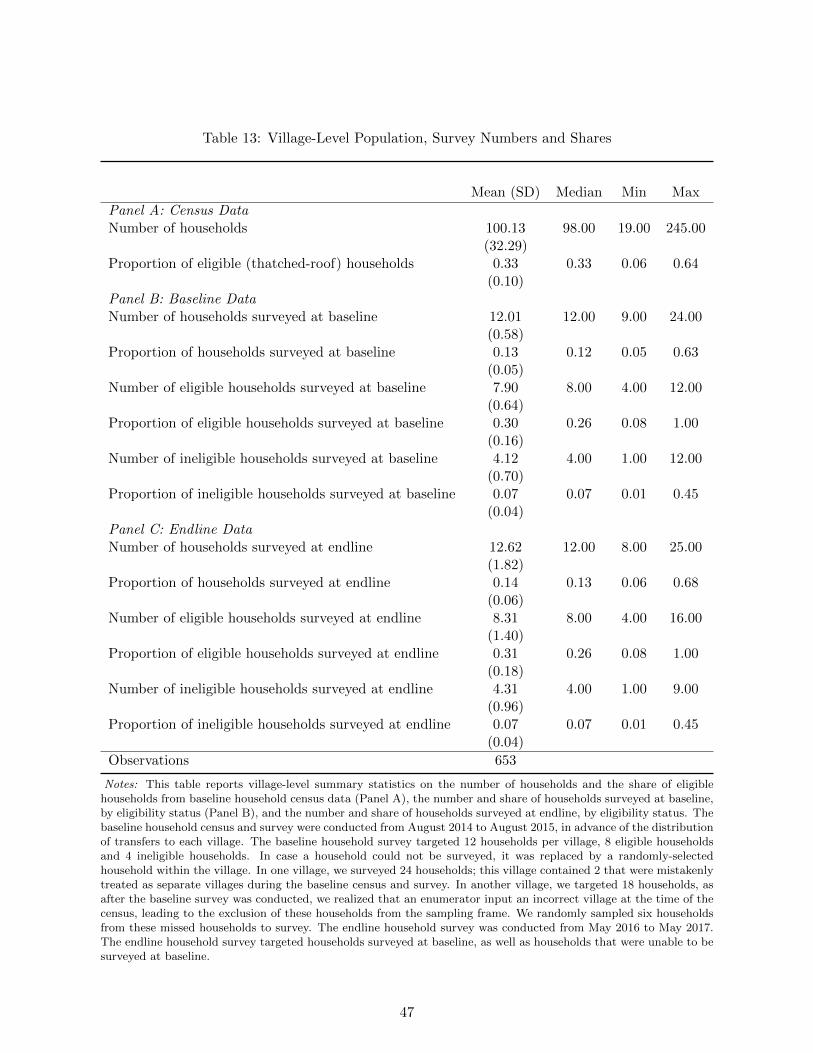
Table 13: Village-Level Population, Survey Numbers and Shares

Mean (SD) Median Min Max

Panel A: Census DataNumber of households 100.13 98.00 19.00 245.00

(32.29)Proportion of eligible (thatched-roof) households 0.33 0.33 0.06 0.64

(0.10)Panel B: Baseline DataNumber of households surveyed at baseline 12.01 12.00 9.00 24.00

(0.58)Proportion of households surveyed at baseline 0.13 0.12 0.05 0.63

(0.05)Number of eligible households surveyed at baseline 7.90 8.00 4.00 12.00

(0.64)Proportion of eligible households surveyed at baseline 0.30 0.26 0.08 1.00

(0.16)Number of ineligible households surveyed at baseline 4.12 4.00 1.00 12.00

(0.70)Proportion of ineligible households surveyed at baseline 0.07 0.07 0.01 0.45

(0.04)Panel C: Endline DataNumber of households surveyed at endline 12.62 12.00 8.00 25.00

(1.82)Proportion of households surveyed at endline 0.14 0.13 0.06 0.68

(0.06)Number of eligible households surveyed at endline 8.31 8.00 4.00 16.00

(1.40)Proportion of eligible households surveyed at endline 0.31 0.26 0.08 1.00

(0.18)Number of ineligible households surveyed at endline 4.31 4.00 1.00 9.00

(0.96)Proportion of ineligible households surveyed at endline 0.07 0.07 0.01 0.45

(0.04)

Observations 653

Notes: This table reports village-level summary statistics on the number of households and the share of eligiblehouseholds from baseline household census data (Panel A), the number and share of households surveyed at baseline,by eligibility status (Panel B), and the number and share of households surveyed at endline, by eligibility status. Thebaseline household census and survey were conducted from August 2014 to August 2015, in advance of the distributionof transfers to each village. The baseline household survey targeted 12 households per village, 8 eligible householdsand 4 ineligible households. In case a household could not be surveyed, it was replaced by a randomly-selectedhousehold within the village. In one village, we surveyed 24 households; this village contained 2 that were mistakenlytreated as separate villages during the baseline census and survey. In another village, we targeted 18 households, asafter the baseline survey was conducted, we realized that an enumerator input an incorrect village at the time of thecensus, leading to the exclusion of these households from the sampling frame. We randomly sampled six householdsfrom these missed households to survey. The endline household survey was conducted from May 2016 to May 2017.The endline household survey targeted households surveyed at baseline, as well as households that were unable to besurveyed at baseline.

47

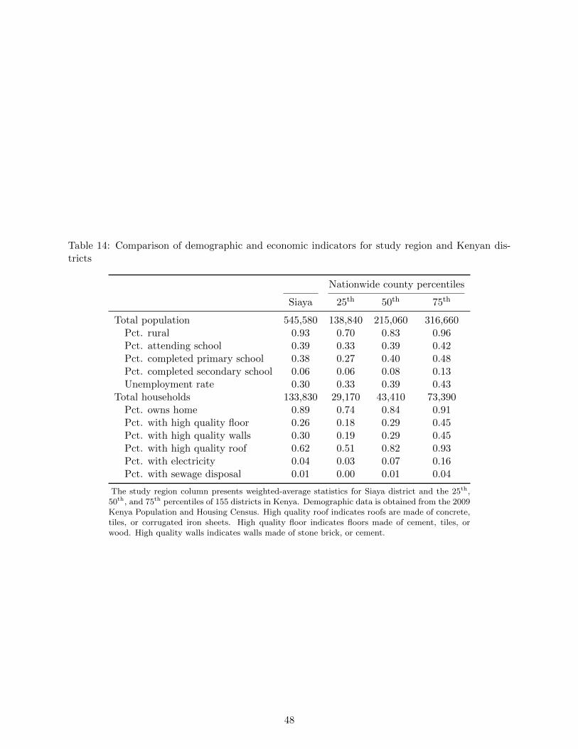
Table 14: Comparison of demographic and economic indicators for study region and Kenyan dis-tricts

Nationwide county percentiles

Siaya 25th 50th 75th

Total population 545,580 138,840 215,060 316,660Pct. rural 0.93 0.70 0.83 0.96Pct. attending school 0.39 0.33 0.39 0.42Pct. completed primary school 0.38 0.27 0.40 0.48Pct. completed secondary school 0.06 0.06 0.08 0.13Unemployment rate 0.30 0.33 0.39 0.43

Total households 133,830 29,170 43,410 73,390Pct. owns home 0.89 0.74 0.84 0.91Pct. with high quality floor 0.26 0.18 0.29 0.45Pct. with high quality walls 0.30 0.19 0.29 0.45Pct. with high quality roof 0.62 0.51 0.82 0.93Pct. with electricity 0.04 0.03 0.07 0.16Pct. with sewage disposal 0.01 0.00 0.01 0.04

The study region column presents weighted-average statistics for Siaya district and the 25th,50th, and 75th percentiles of 155 districts in Kenya. Demographic data is obtained from the 2009Kenya Population and Housing Census. High quality roof indicates roofs are made of concrete,tiles, or corrugated iron sheets. High quality floor indicates floors made of cement, tiles, orwood. High quality walls indicates walls made of stone brick, or cement.

48

B.1 GD’s Program

GD’s enrollment process in treatment villages consists of the following 6 steps:

1. Village Meeting (baraza): before beginning work in a village, GD holds a meeting of all

households in the village to inform villagers that GD will be working in their village, explain

their program and GD as an organization. To prevent gaming, the eligibility criteria are not

disclosed.19

2. Census: GD staff conduct a household census of the village, collecting information on house-

hold names, contact information and housing materials. The information on housing materials

are used to determine program eligibility.

3. Registration: Households identified as eligible based on the household census are visited by

the registration team. GD staff confirm the eligibility of the household, inform the household

of their eligibility for the program and register the household for the program. This is the

point at which households learn they will be receiving transfers, as well as the amount of the

transfers, the transfer schedule, and the fact that the transfer is unconditional.20 For couples,

the couple decides which individual will be designated as the recipient. The member of the

household identified as the recipient is instructed to register for M-Pesa in their name, a

prerequisite for receiving the transfer. Households that do not have a mobile phone are given

the option to purchase one from GD staff, the cost of which is deducted from the transfer

amount. Even if the household does not own a phone, the individual recipient can still register

for M-Pesa with a SIM card; the SIM card can then be inserted into any phone in order to

make withdrawals.

4. Backcheck: All registered households are backchecked to confirm eligibility in advance of the

transfers going out. This is an additional step to prevent gaming by households and field

staff, as the census, registration and backcheck teams consist of separate staff members.

5. Transfers: The cash is transferred in a series of three payments via M-Pesa according to the

following schedule: (i) the token transfer of KSH 7,000 (about USD 70) ensures the system

is working properly; (ii) two months afterwards, the first lump sum transfer of KSH 40,000 is

distributed; (iii) six months after this, the second and final lump sum transfer of KSH 40,000

is sent.21 Transfers are typically sent at one time per month to all households scheduled to

receive transfers.

19. However, the eligibility criteria is not difficult to deduce given that it is publicly observable, and anecdotallymany households in the study area are aware of targeting criteria.

20. To emphasize the unconditional nature of the transfer, households are provided a brochure with many potentialuses of the transfer.

21. If households elected to receive a mobile phone from GD, the cost of this is taken out of the second lump sumtransfer.

49

6. Follow-up: After transfers go out, GD staff follow up via phone with transfer recipients to

ensure no problems have arisen. In addition, there is a GD help line that recipients can

contact. If GD staff learn that household conflicts have arisen as a result of the transfers,

subsequent transfers may be delayed while these conflicts are worked out.

50