Informal insurance in the presence of poverty traps: Evidence

Informal insurance in the presence of poverty traps:

Evidence from southern Ethiopia

Paulo Santos Ph.D. Student, Cornell University

Christopher B. Barrett International Professor, Cornell University

Contributed paper prepared for the 26th Conference of the

International Association of Agricultural Economists

Brisbane, Australia, 12-18 August 2006

© Copyright 2006 by Paulo Santos and Christopher B. Barrett. All rights reserved. Readers may make verbatim copies of this document for non-commercial purposes by any means, provided that this copyright notice appears on all such copies.

1

Informal insurance in the presence of poverty traps:

Evidence from southern Ethiopia

Abstract: Recent empirical work finds evidence of highly nonlinear wealth dynamics among Boran pastoralists of southern Ethiopia, consistent with the hypothesis of poverty traps. This paper explores the consequences of such dynamics for informal inter-household transfers. Using original primary data on social networks and transfers, we find that asset transfers respond to recipients’ losses, but only so long as the recipients are not “too poor”. The persistently poor are excluded from social networks and do not receive transfers in response to shocks. We also find some evidence that the threshold at which wealth dynamics bifurcate may serve as a focal point at which transfers are concentrated. This suggests that asset transfers, in the context of poverty traps, may aim to insure the permanent component of income generation, rather than the transitory component, as standard insurance models assume.

Keywords: risk, informal insurance, social networks, poverty traps, Ethiopia

JEL codes: Z13, I3, O13

2

1. Introduction

Risk is a central feature of life in rural areas of developing countries. Economic

theories of risk sharing, rooted in the work of Arrow (1964), Diamond (1967) and Wilson

(1968), posit that individuals will use a variety of instruments – most notably for our

purposes, informal insurance based on interhousehold transfers (Townsend 1994, Lim

and Townsend 1998) – to shield consumption from the idiosyncratic variation in income

that is commonplace in these settings. Models of informal insurance are based on the

strong, if often only implicit, assumption that the income generating process is stationary

or, in other words, that shocks only have transitory effects. For example, Coate and

Ravallion (1993, p.4) justify their focus on symmetric insurance arrangements with the

assumption that “either player could end up ‘rich’ or ‘poor’ in any period” with equal

probability.1 The assumption that income processes are stationary provides the basis for

an all-inclusive insurance pool.2

Yet a growing literature, recently reviewed by Azariadis and Stachurski (2004),

emphasizes the possibility of nonstationary income processes that may yield multiple

dynamic equilibria, with one or more stable equilibria below the poverty line – a low-

level equilibrium (poverty) trap.3 What implications, if any, might poverty traps have for

the functioning of informal insurance networks?

1 The same assumption is true in Ligon et al. (2002) in the case of nonstationary transfers. 2 The next section discusses some models that emphasize limits on the size of the insurance group without abandoning the assumption of stationary income processes. 3 Some of this literature emphasizes the role of uninsured risk as a as a root of poverty, generally emphasizing the role of ex ante choices and intended to diminish the impact of shocks (e.g., Binswanger and Rosenzweig 1993, Bardhan, Bowles and Gintis 2000, Carter and Barrett 2006). See Dercon (2004) for a review of this relation.

3

The theoretical literature on poverty traps posits the rational exclusion of the poor

from welfare-improving opportunities, such as informal insurance contracts. This occurs

because, under limited commitment, agents must use informal sanctions to ensure that

contracts are respected and sanctions have less “bite” for those who have little to lose

(Banerjee and Newman 1995). This is not, however, the only possible rationale for being

selective about with whom to insure.

In the presence of multiple dynamic equilibria, small transfers can have large

welfare impacts if, in the wake of a shock with potentially long lasting or permanent

effects,4 they succeed in making the recipient cross the unstable dynamic equilibrium at

which path dynamics bifurcate. If a poverty trap exists, then the unstable dynamic

equilibrium may serve as a focal point for interhousehold asset transfers since this is the

point at which the long-term welfare impact of a transfer is greatest. Transfers might then

be appropriately conceptualized as a mechanism to defend households from falling onto a

path of sustained asset loss and eventual destitution. Although the available data do not

allow a conclusive test between these two models, we present evidence based on

simulations of expected wealth dynamics that seems to favor this latter explanation.

The remainder of the paper proceeds as follows. Section 2 briefly outlines a

simple model of informal insurance in the presence of poverty traps that shows how the

resulting patterns of interhousehold transfer may differ from the stationary case of an all-

inclusive insurance pool, with wealth playing a central role in determining who is and is

not included. Section 3 then introduces the setting we study and the data we use,

4 The possibility that shocks may have long lasting or even permanent effects is addressed in, for example, Martorell (1999), Ravallion and Lokshin (2005), Dercon (2004) and Dercon and Hoddinott (2004). In our case, such shocks would be those that leave the individual below the path dynamic threshold.

4

collected from southern Ethiopian Boran pastoralists, a population among which

nonlinear wealth dynamics characterized by poverty traps has been reasonably well

established (Lybbert et al. 2004, Santos and Barrett 2006a). In section 4 we study

informal insurance links among the Boran and find that respondents’ decision to give

cattle to an individual is not unconditionally triggered by the prospective recipient’s

losses – as it would in the canonical insurance model – but depends on the match’s losses

conditional on herd size – as a model that takes into consideration the existence of

poverty traps would predict. This result is robust to a series of additional controls, namely

for individual-specific ability that Santos and Barrett (2006a) find influences herd

dynamics. We further explore whether these decisions seem to be influenced by a

prospective transfer recipient’s position relative to the unstable asset equilibrium – the

accumulation threshold identified by Lybbert et al. (2004) and corroborated by Santos

and Barrett (2006a) – by analyzing the effect of two variables that may drive the

propensity to reciprocate gifts (expected wealth and expected gains from gifts). We find

evidence of non-monotonic relation between matches’ wealth and the formation of

insurance links. In section 5 we then study patterns of social acquaintance and find that

wealth plays a role in explaining who is known within a community and thus who can

mobilize transfers in response to shocks. Being destitute has a strong, negative impact on

the probability of being known and, since cattle transfers only occur between people who

know each other, persistent poverty thereby becomes socially invisible. Finally, section 6

summarizes these results and draws out the policy consequences of our findings.

2. Transfers in the context of poverty traps

5

A simplified version of the intertemporal decision problem facing a risk-averse

agent i, in which utility is defined over wealth and we rule out bequest motives for

accumulation can be written as:

(1) max{Jt} E { 3t= 0…T $t U(ki

t) | N(C)}

subject to: kit = g( ki

t-1 (1+ Nit (ki

t-1)) + Jijt + Jji

t)

ki0 given

kiT = 0

where kit stands for the agent’s assets, our state variable, Jt represents transfers (negative

if given to some other agent j, Jijt, positive if received from another, Jji

t) and Nit (ki

t-1) is a

shock drawn from the distribution N(C) with support on the interval [-1, 0], reflecting

losses that could range from 0-100% of i’s initial asset stock. This formulation highlights

both the importance of self-insurance (through ex ante asset levels, that affect the

probability distribution function of shocks5) and the role of informal insurance. Because

theoretical models of poverty traps emphasize the role of asset accumulation in shaping

welfare dynamics, we focus on asset shocks and transfers rather than on income shocks,

as is more common in the literature on informal insurance.6

The growth function that underlies the asset law of motion, g(C), must be general

enough to incorporate two possibilities, identified in earlier work in this environment

5 As Lybbert et al. (2004) report, sales and slaughtering are tiny, less than two percent of herd, on average, among the population we study Thus shocks (mainly mortality) are almost the unique reason for decreases in herd size, while increases are mostly due to biological reproduction. The importance of asset levels in determining the level of risk has the paradoxical effect that asset levels, in this economy, are (to a large extent) exogenously determined. Clearly, the simplicity of this economy facilitates the econometric analysis to a degree that would be harder to achieve in other contexts, where we may suppose that the role of agency in dealing with shocks (in choosing the level of risk to which one is exposed or to invest in formal financial instruments, for example) is potentially much larger. 6 An exception is the analysis in McPeak (forthcoming). McPeak (2004) also argues that income and asset shocks, albeit correlated, can have different (and offsetting) impacts on household behavior (asset sales).

6

(Santos and Barrett 2006a). First, household characteristics (e.g., intrinsic ability) may

sort cross-sectional units into distinct cohorts or clubs, c. Second, within each club,

agents might face nonstationary dynamics – in particular, and as hypothesized by

multiple equilibrium models, the possibility of a critical threshold value, (c, at which the

welfare dynamics bifurcate, with one path, subscripted ℓ, leading to a low-level

equilibrium and another, subscripted h, leading to a high-level equilibrium. These

possibilities imply that for each club c=1,…, C , the asset law of motion is

Borrowing the terms from the growth literature, this specification can be

simplified into a club convergence approach (as in Quah 1997) if there are no asset

thresholds at which asset dynamics bifurcate (that is, (c=0, œc), or into a threshold model

(as in Azariadis and Drazen 1990) if there is only one club (that is, C=1).7 If one assumes

that g(C) is concave, and that there are no convergence clubs or thresholds, we’re back to

the convergence model of Solow (1956) that, implicitly, underlies the consumption

smoothing literature with its assumption of a stationary income process.

The insurance contract available to these agents is very simple and formally

defined by Jijt = {J, 0} that is, at each period t, agent i can transfer to agent j a fixed

amount of assets (J) or nothing at all. This dichotomous treatment of transfers is a

reasonably accurate description of the reality of asset transfers in the setting we study

7 Several approaches have been recently suggested to identify convergence clubs (for example, Canova 2004) and thresholds (for example, Hansen 2000) but not, to our knowledge, both. In the empirical section we’ll build on previous work (Lybbert et al. 2004, Santos and Barrett 2006a) to identify both convergence clubs and accumulation thresholds.

gcℓ(kt-1 (1+Ni

t ( kt-1)) + Jjit + Jij

t ) if i0c, kt-1 < (c (2) kc

t= 9 gch(kt-1 (1+Ni

t ( kt-1)) + Jjit + Jij

t ) if i0c, kt-1 $ (c

7

(see section 3) and reduces the demand for insurance to a binary decision of whether to

insure with a specific partner or not – in other words, to a process of dyad formation.

Keeping with the extant literature on informal insurance, we assume that the

motivation for entering such contract is “balanced reciprocity” (Platteau 1997), ruling out

altruistic reasons for such transfers. The simplest structure that allows for such a

motivation must span two periods. In period 1, agents play a two-stage game. In the first

stage, shocks are revealed to each agent and an agent j who has suffered a herd loss

approaches i with a request for a transfer of τ. In the second stage, i decides whether or

not to accept the request – that is, whether to form an insurance link with an agent.8

Growth then occurs. Then in period 2, transfers are reversed and j transfers τ back to i.9

This is obviously a simplification of complex informal insurance systems, but it captures

the essential elements: dependence on the conscious choice to form and/or activate a

dyadic link, state-contingent transfers, and eventual reciprocation.

Given this structure, transfers will be made if the expected gains from transfer

over autarky are strictly positive

(3) Jij1 = J iff EUi(J) > EUi(0)

where

(4) EUi (•) = EUi

1 (•) + $ EUi

2 (•) * 1(Jji

2=J)

8 Note that we model the insurance link formation as occurring ex post of the shock – rather than ex ante of the shock, as is more common in the literature – in order that the structure of the model matches that of the data we use in section 4. 9 One can equally conceptualize τ as a loan, a gift or an insurance payment. As we discuss below, these are observationally equivalent in the data we use.

8

and $ < 1 is the time discount rate. Uncertainty about whether such gifts will be

reciprocated, given their informal nature, is usually addressed through an appeal to the

theory of repeated games. We summarize such game-theoretic structure by the function

1(Jji2=J) that expresses the probability that, in period 2, agent j will reciprocate the

original gift as a result of the rules in place, with 1(Jji2=J) = 1 meaning that such

contracts are perfectly enforceable.

This paper explores what changes in the structure of insurance networks might

arise from the introduction of multiple equilibria, as in equation (2). More concretely, we

ask: do herd dynamics guide the selection of insurance partners?10 In what follows, we’ll

see that the answer is “no” in the convergence model and “yes” in a model with multiple

equilibria.

2.1 Stationary dynamics: convergence towards one equilibrium

Let ke be the dynamic equilibrium asset value for which kt=kt-1 and consider the

case of no clubs, g(C) a strictly concave function on assets and g(0) > 0. It is easy to show

that ke is unique and it is clear that, as T64, the distribution of assets among the

population will converge to a degenerate distribution characterized by prob(k=ke)=1,

regardless of the initial distribution of assets among the population. Starting from that

10 At least three recent papers explore similar questions. Zimmermann and Carter (2003) show that in the face of income shocks, individuals near a critical asset threshold will tend to preserve or smooth their assets, destabilizing consumption in order to avoid an intertemporally costly collapse below the threshold. Following the same argument, Hoddinott (2006) shows that asset sales (oxen and cows/heifers) by Zimbabwean farmers depend on their position relative to an asset threshold (of two oxen, in this sample), with those above the threshold selling far more frequently in response to idiosyncratic shocks. Barrett et al. (2006) show, using data on pastoralists from northern Kenya, that income and consumption smoothing behavior are differentiated by wealth, with poorer households suppressing income variability while wealthier ones smooth consumption, a pattern consistent with the idea that the most vulnerable households destabilize consumption in order to protect crucial productive assets on which their future survival depends.

9

equilibrium, we need only to concern ourselves with negative shocks: in a way analogous

to the discretization applied above to the possible contracts, let the shock be defined by

the pair Nit 0 {0, N}, with -1 < N < 0, each state occurring with non-zero probability. Let

the growth function be defined by

(5) g(ke (1+ Nit (ki

t-1)) | Nit =0) = g(ke - Jij) = ke


t-1)) | Nit = N) = ke + N + H


t-1)) + Jji | Nit = N) = ke.

with 0 < H < |N| . With agents starting at the equilibrium ke, the value of setting Jt=J is to

hasten convergence towards ke if one suffers a negative shock. Given that transfers are

small relative to the equilibrium ke, convergence reoccurs in a single period, as reflected

in equation (5). It is clear that EUi(J) > EUi(0) holds for any individual. Hence, the

insurance pool will include all agents. The key point here is that when the underlying

stochastic process is stationary (and abstracting from the costs of contracting), there is no

reason to exclude prospective insurance links from one’s network.

2.2 Non-stationary dynamics: the possibility of multiple equilibria

Consider now a growth club with multiple equilibria, ke={kl, (, kh}, with kl

representing the low-level stable equilibrium, kh representing the high-level stable

equilibrium, and ( the (unstable) threshold at which the accumulation dynamics

bifurcate, per equation (2). The transition matrix between these equilibria is presented in

Table 1. Each cell represents the probability of each asset position after the period 2

shock – i.e., at the point at which j would reciprocate with a transfer of τ back to i – (the

10

columns), given the first period shock (the rows). Table 1 thus captures the one period

ahead wealth distribution at the moment i would ask j to reciprocate, conditional on asset

holdings at the time j approaches i for a transfer of τ.

The speed of transition towards the nearest stable equilibrium is captured by ε. If

ε>0, as we’ll maintain throughout the analysis, then the system is ergodic.11 In the long

run, everyone has a non-zero probability of spending time in both stable equilibria and

initial conditions no longer matter. In a stricter definition that equates history dependence

with lack of ergodicity, this is no longer a model of poverty traps. Note however that if

one starts at the low-level equilibrium, then ε is also a measure of the degree of poverty

persistence. If, as we also assume, ε is small, then transitions between stable equilibria

are possible but the poor may spend a long time in the low-level equilibrium.12 This

approach adds realism to the analysis, by avoiding a deterministic model where poverty

traps are absolute and can never be overcome, without necessarily diminishing the policy

relevance of the existence of multiple equilibria.

We also assume that *, the probability of ending up at the low-level equilibrium

if, ex post shock, one is at ( is higher than :, the probability of the same end result if one

is above the threshold when growth occurs. To make the problem interesting, we further

assume that kl + J < ( (a poor agent cannot reach the threshold through transfers) and kh -

J > ( (a wealthy agent does not compromise his growth capacity by transferring J to an

insurance partner).

11 More rigorously, we could have considered εl ¸ εh, and we would only need to assume that εl > 0 to get an ergodic system. This would overburden the notation with insignificant changes in the results. 12 Mookherjee and Ray 2001 label this process “self-reinforcement as slow convergence”. The definition of poverty trap adopted by Azariadis and Stachurski (2004, p. 33) - “A poverty trap is any self-reinforcing mechanism which causes poverty to persist” - explicitly allows for this approach.

11

Limited commitment translates into 1(Jji2=J) < 1. Can we then expect a higher

probability of defaulting from particular types of prospective transfer recipients? Given

that marginal utility is decreasing in k, the punishment strategies that make such contracts

feasible are less effective when applied to those with less wealth. Because default on the

same transfer yields greater utility for those with less wealth,13 an ordering of agents

emerges that is (weakly) monotonic in wealth space:

(8) 1(Jji2=J| kl) # 1(Jji

2=J | () # 1(Jji2=J | kh)

This corresponds to the usual reasoning about incentives and behavior in the

context of persistent poverty (Banerjee and Newman 1994, Banerjee 2000). McPeak

(forthcoming) takes this line of argument one step further, suggesting that asset transfers

in a context quite similar to the one we study can be understood as ex ante precautionary

savings rather than as ex post insurance. In this case, only capacity to reciprocate the gift

should matter to the decision to transfer assets that would be independent of the

realization of a (negative) shock by the prospective recipient. One can test this prediction

empirically, as we do below.

A plausible modification to this model explores the idea that the receiver’s

valuation of the original transfer may affect his decision not to default, as in the empathy

formation model proposed by Stark and Falk (1989). If higher valuation of the transfer by

13 An extreme version of the argument follows from the (ad-hoc) assumption that u(kl-J) = - g. In this case, it is clear that those with asset stocks of kl will renege on the contract in period 2 and we only need to compute the probability of holding kl at period 2, conditional on asset levels in period 1, to rank the agents in terms of their desirability as insurance partners: [1(Jj2=J |kj1 = kl) = ε] < [1(Jj2=J |kj1 = \) = 1 - ^ - ^ε] < [1(Jj2=J |kj1= kh) = 1 - n- nε]. Note that without such certainty about defaulting, we can only use weak inequalities, as done above.

12

the original recipient leads to a smaller probability of default, due to “gratitude” or

similar emotions,14 then we can write

(9) 1 (Jji2=J) = f(Vj(Jij

1=J))

where Vj(C) is j’s valuation of the transfer made in period 1 and f(•) is an increasing

function. We can write Vj(C) as a function of the gains, in terms of growth, from the

initial transfer:

(10) Vj(Jij1=J) = gj

1 (kj (1+ Nit (ki

t-1)) + Jij1) – gj

1 (kj (1+ Nit (ki

t-1))

Given the structure of the growth process, it is straightforward to show that

(11) V(kl) = 0

(12) V(() = (:– *) (1-ε) (kl – kh) > 0

(13) V(kh) = 0

As a consequence, 1(kl) = 1(kh) < 1((). A gift will be valued if, ex post shock, the

potential recipient is at ( given that only then can transfers influence the equilibrium to

which the recipient converges. If the receiver’s valuation of the gift affects propensity to

reciprocate, the ordering of preferred agents to whom one makes transfers becomes non-

monotonic in the wealth space, with the maximum at the unstable equilibrium, (.

Several other explanations from the literature merit some attention, given their

attempt to explain rational selection out of insurance contracts. The closest to our analysis

is by Hoff (1997), who predicts matches along wealth levels. Individuals with high

14 See Komter (2005) and references therein on the role of gratitude as the “moral memory of mankind” and the psychological foundation for reciprocity and Hirshleifer (1987) for a discussion of the role of emotions as guarantors of contracts.

13

enough expected wealth may not invest in insurance relations because the expected

benefits may not compensate for expected net contributions to the insurance pool. This

result implicitly depends on the lack of convergence in incomes between agents (some

have higher expected income than others) and relies heavily on the impossibility of

separating insurance from redistribution due to egalitarian sharing rules, an environment

quite different from the one that we study. In section 4 we test this model, since we use

data from both sides of the insurance contract and control for the giver’s wealth.

Given that informal transfers can insure only against idiosyncratic shocks – not

against covariate ones – asset covariance between potential insurance partners should

matter to contracting choices, as the related literature on peer selection in micro-credit

arrangements suggests (Ghatak 1999, Sadoulet and Carpenter 1999). Agents might

therefore rationally opt out of insurance contracts with those whose wealth covaries

strongly with their own wealth. We address this possibility below, as an additional check

on our results.

Finally, Murgai et al. (2002) suggest that the costs of establishing insurance links

may limit the domain of insurance links. Genicot and Ray (2003) likewise suggest that

insurance groups may be bounded because risk-sharing arrangements need to be robust to

deviations by sub-groups. Although these arguments do not explicitly model wealth as a

source of friction that might prevent insurance links from forming, they offer

complementary explanations for the behavior that we observe. In our empirical work, we

therefore control for covariates that may reflect differences in the degree of enforcement

14

of such contracts or in the monitoring of other agent’s activity and, less perfectly, for the

degree of alternative insurance ex ante of the link formation decision.15

3. Boran pastoralists in southern Ethiopia

Lybbert et al. (2004) analyze wealth dynamics among Boran pastoralists, a poor

population in southern Ethiopia. Using herd history data for 55 households over a 17 year

period, they show that herd dynamics follow a S-shaped curve with two stable equilibria

(at approximately 1 and 35-40 cattle), separated by an unstable threshold (at 15-20

cattle). The authors suggest that this threshold results from a minimum critical herd size

necessary to undertake migratory herding to deal with spatiotemporal variability in forage

and water availability. Those with smaller herds are forced to stay near their base camps,

where pasture conditions soon get degraded, leading to a collapse of herd size towards

the low-level stable equilibrium, while those with bigger herds can migrate in search of

adequate water and pasture, enabling them to sustain far larger herds.

Two other findings presented in Lybbert et al. (2004) help motivate this paper.

First, they show that asset risk is predominantly idiosyncratic. This creates conditions

conducive to the implementation of welfare-improving insurance contracts among

pastoralist households. Second, they find that insurance operationalized through inter-

15 The relevance of Genicot and Ray (2003) is questionable in our context, given that we address the issue of network formation. Groups differ from networks because of the existence, in the latter, of a common boundary: if A establishes a link with B, the fact that B already has a link with C does not mean that A will also have a (direct) link with C. Hence considerations about sub-group deviations may be less of a concern here than in more formalized institutions such as, for example, the funeral insurance groups studied by Bold (2005).

15

household gifts and loans of cattle are conspicuously limited. On average, a household

must lose 30 cattle more than the community average herd loss in order to trigger the

transfer of a single cattle.

This meager insurance payment, corroborated by other recent studies from semi-

arid African systems (Kazianga and Udry 2006, Lentz and Barrett 2005, McPeak 2005),

seems paradoxical in the face of overwhelmingly idiosyncratic insurance risk: why would

people bypass so many opportunities to trade? We hypothesize that one of the reasons

may be the rational exclusion of some of members of society from such contracts due to a

correct understanding of the nonlinear wealth dynamics in this economy.16

We employ two datasets. The first consists of household survey data collected

from 119 randomly selected Boran pastoralist households in four communities of

southern Ethiopia.17 These data on pastoral risk management (PARIMA) were collected

every three months, March 2000-June 2002, and then annually each September-October

starting in 2003, and include rich detail on household composition, education attainment

(although very few respondents are literate or attended any school), migration histories,

changes in herds, shocks, etc.

The second data set includes observations of these same households’ stated

choices of insurance matches. In order to identify the determinants of interhousehold

transfer arrangements, we randomly matched each respondent with other respondents

16 Santos and Barrett (2006a).show that our respondents indeed perceive such dynamics . 17 The data were collected by the Pastoral Risk Management (PARIMA) project of the USAID Global Livestock Collaborative Research Support Program. Barrett et al. (2004) describe the location, survey methods and available variables.

16

from the PARIMA sample and asked two types of questions:18 the first about (real) social

acquaintance (“Do you know (name of the match)?”), the other on the possibility of

transferring cattle as a gift if the match asked for it.19 The latter question provides

information on potential transfer networks and is the subject of study in the next section.

This approach offers one major advantage and two prospective disadvantages

relative to previous studies of informal transfers. Because we know the characteristics of

both giver and recipient, no questions of bias arise with respect to the estimates of the

transfer function due to lack of knowledge about one end of this relation (Rosenzweig

1988, Cox and Rank 1992). However, there are two prospective problems with this

approach. First, by studying links between individuals rather than the transfers

themselves, one risks errors due to excessive discretization. However, this is not a

problem in our data because informal asset transfers among Boran pastoralists are quite

small. In our sample, over the period 2000-03, there were 15 such transfers, out of which

12 (i.e., 80%) were of 1 or 2 cattle.20 For that reason, and with only a slight abuse of

language, we use the terms “network formation” and “transfers” interchangeably in what

follows.

Second, one might reasonably wonder how well potential transfer networks

elicited in this manner reflect the decision process underlying the formation of real

18 This approach follows closely the one used by Goldstein and Udry (1999) in Ghana. Granovetter (1976) had earlier proposed a similar approach. 19 We asked also about the possibility of transferring cattle as loans but the pattern of answers is virtually identical and gifts and loans seem empirically indistinguishable. Out of 561 matches, in only 13 (2.3%) does the decision differ between loans and gifts. We therefore concentrate on transfers deemed “gifts” in what follows. 20 A separate survey of cattle transfers motivated by shocks, conducted in 2004, in the same geographical area but with different respondents, suggests even greater dominance of small transfers: out of 112 transfers, 102 (or 91%) were of 1 cattle, 8 (or 7%) were of 2 cattle and the remaining less than 2% were more than 2 cattle.[0]

17

insurance networks. In a separate paper (Santos and Barrett 2006b) we show that

inference with respect to the determinants of insurance networks derived from the

approach used in this paper closely match those obtained from analysis of real social

relations among the same population. The appeal of using randomly matched respondents

thus seems to outweigh the prospective pitfalls of using discrete data on hypothetical

transfers.21

4. Poverty traps and social transfer networks

The basic pattern of answers to the stated insurance link questions is described in

Table 2. Three key facts emerge clearly. First, not everyone knows everyone else, even

in this rural, ethnically homogeneous setting in which households pursue the same

livelihood and there is very little in- or out-migration. Although most people know the

random match presented to them, almost 14% of the matches were unknown by the

respondent. Second, social acquaintance is, for our respondents, clearly a necessary

condition for willingness to make a transfer.22 In only 3/68 cases did a respondent

indicate that they would be willing to give livestock to someone they did not know. This

makes the explanation of who knows whom – and, its corollary, social invisibility, i.e.,

who is unknown by others – an important question unto itself, one that we explore in

section 5. It also implies an apparently sequential problem that leads us to estimate the

21 The benefits of using experimental data in the study of social capital (a concept closely related with that of social networks) is emphasized by Durlauf and Fafchamps (2004). Glaeser et al. (2000) and Barr (2003) both conclude that experimental evidence is mirrored by reality. 22 Of course one can imagine situations where this would not hold (for example, someone may address a local patron and seek to put himself under his protection or someone may seek the help of friends of friends, even when they were not previously acquainted). Although theoretically possible, these do not seem to find support in our data.

18

determinants of transfer networks only on the subsample of those who know their match

(Amemiya 1974, Maddala 1983). Finally, knowing people is by no means a sufficient

condition for pastoralists to be willing to transfer animals to a match. In just under one

quarter of the cases where the respondent knew the match was he or she willing to give

an animal to the match. The acquaintance between giver and receiver seems therefore to

be necessary but insufficient for mobilizing support.

The intuition behind these responses is that respondents perform a cost-benefit

analysis with respect to each potential link/gift before deciding whether to give cattle

when asked for it, answering “yes” if their subjective evaluation of the benefits exceeds

the costs. The question then becomes what process governs that calculus.

Under the canonical model of informal insurance and consumption smoothing,

assuming a stationary asset process, transfers should be unrelated to one’s asset stocks

and depend solely on a prospective recipient’s losses relative to the insurance group

mean. Thus matches with different herd sizes should be equally likely to receive

transfers conditional on a similar loss experience, following the simple model in section

2.1. Transfers would depend on above-average losses alone. Under McPeak’s

(forthcoming) alternative formulation, the likelihood of making a transfer should be

increasing in a match’s herd size since wealthier partners are more likely able to

reciprocate in the future, and past experience of shocks by the match should have no

effect on transfers.

The model of informal insurance under non-stationary dynamics, sketched out in

section 2.2, offers a different set of predictions: transfers should respond to shocks

conditional on ex post herd size. And unlike McPeak’s precautionary transfers model,

19

they should be invariant with respect to herd size in the absence of a shock. These

contrasting predictions, summarized in Table 3, enable us to test which model of informal

insurance seems to best fit these data in an area where the existence of a poverty trap has

now been reasonably well established.

Because these households have been observed repeatedly since 2000, we can use

actual herd size observations for each respondent and his random match to test between

these competing hypotheses. The key variables then become (i) herd position with respect

to the different equilibria identified in Lybbert et al. (2004) and corroborated in Santos

and Barrett (2006a), (ii) whether or not the match lost cattle, and (iii) match’s herd size.

As described in Table 4, we get at (i) by constructing four dummy variables that provide

a categorical representation of household-level expected herd growth in the period after

the survey on social transfers. A household falls in category E1 if it lies in the

neighborhood of the low-level stable equilibrium, with a herd of less than five cattle in

2003. It belongs in category E2 if it lies just below the threshold at which herd dynamics

bifurcate, with a herd of 5-14 cattle. If the herd size was above the unstable equilibrium

but beneath the high-level equilibrium (15-39 head), the household was classified as

belonging to group E3. Finally, households with herd sizes at or above the high-level

stable equilibrium (40 or more) were assigned to E4. We capture variable (ii), herd loss,

through a dummy variable, Lj, taking value one if the match (j) had a smaller herd in

2003 than in 2000, and zero otherwise.23

23 Note also that given that in all communities, growth was positive in this period, there would be no change in results if we had defined this variable has taking the value 1 if the respondent had registered a loss above the one registered by the community, since all communities experienced net herd gains over this period. This would be a more precise way of defining idiosyncratic risk, although at the cost of making the implicit assumption of equivalence between insurance pool and the community used in the sampling strategy.

20

We then study respondents’ decision to make a gift or not using a model that nests

the different explanations/motives for asset transfers under the reduced form

(14) lij* = αi + (1 f(hj) + H Lj + Σ t=1…4 βt Etj + δ Xij + λZi + εij

where lij* is the propensity to establish a link between i (the respondent) and j (the match),

hj is the match’s herd size, the X vector captures a range of covariates describing the

relation between i and j, and the Z vector reflects attributes of the respondent, such as

age, household labor supply and village of residence. If we define lij = 1 as the actual

realization of the variable lij* when a link is formed and assume that

(15) εij ~ log(0, π2/3)

(16) E (εij , εih) ≠ 0 if j ≠ h

(17) E (εih , εjh) = 0 if i ≠ j

we can estimate this as a logit model through clustering of the observations on the

identity of the respondent, premised on the idea that relations are nested within

individuals.

One alternative way of modeling the error term is to incorporate the effect of

match’s unobservables. Both Udry and Conley (2005) and Fafchamps and Gubert

(forthcoming) correct the variance matrix for the possible effect of match’s

unobservables, using Conley’s (1999) estimator, and find that the corrected standard

errors do not differ significantly from estimates that do not account for this effect. We

follow a slightly different strategy, using a nonparametric permutation test known as

Quadratic Assignment Procedure (QAP) (Hubert and Schultz 1976, Krackhardt 1987,

21

1988) to obtain correct p-values.24 We too find that this added control for potential

correlation on unobservables makes no significant difference to our results when

explaining the formation of transfer dyads. However, it does matter when explaining

who knows whom.

The elements of X – clan membership, gender, age, land holdings, cattle holdings,

and household size – are expressed not as the Euclidean distance between the pair but

rather, following Santos and Barrett (2005), using a measure of distance that allows for

ordinal differences in the relative position of respondent and match to play a role in

explaining the respondent’s decision.25 This approach offers an intuitively more

appealing interpretation of the effects of social and economic distance than the more

conventional Euclidean measure of social distance that (implicitly) would impose

symmetry in the effect of these variables upon the dyad formation decision.

Table 5 presents the estimates of the logit regression when the dependent variable

is the decision to give cattle to the match if he/she asked for it. We present several

specifications of this model that differ in the way we express the effects of herd losses

and match’s wealth, thereby allowing testing among the different models outlined above.

24 The basic intuition behind this procedure is that the permutation of the data on the dependent variable must maintain its clustered nature. In practice, this means that the same permutation must be applied to respondents and matches. We can then estimate the above model when all correlation between dependent and independent variables is broken through resampling – that is, when the null hypothesis that all slopes equal zero is known to be true – and compare our first estimates with their empirical distribution obtained through the repetition of this exercise (in our case, 1000 times), to generate a sampling distribution for the parameter estimates. 25 To be more concrete, consider the case of a categorical variable such as gender: we can think of whether match and respondent share the same gender and estimate a dummy variable “same gender” – implicitly imposing that the effect of a female-female match is the same of a male-male one – or we can consider the set of all possible matches (female-female, female-male,…) and estimate a dummy variable for each specific combination. Mutatis mutandis, the same reasoning applies to continuous variables. With a different formalization, the same idea is captured in Fafchamps and Gubert (2006).

22

First, however, let us note a few results with respect to the X and Z variables

defining relational characteristics between i and j and attributes of i, respectively. These

results reflect possible frictions and associated costs of establishing an insurance link

(Murgai et al. 2002) and are robust to the various specifications we report with respect to

herd losses and herd size. The propensity to give a gift is strongly, positively influenced

by belonging to the same clan. Variables that measure social distance in terms of gender

are clearly asymmetric. Men are more willing to give cattle (either to women or to other

men) than are women. The larger one’s household, the more likely the respondent is to

give a gift, although that effect is attenuated when the giver’s household has more

members than the prospective recipient’s. Physical proximity and age have no

statistically significant effect on transfer patterns in these data.26

We now turn to the core hypotheses of interest: the relation between asset

transfers, wealth and asset shocks. Let us start with the simplest specification, in column

(1), in which we test for a relation between herd size and the propensity to make a gift.27

There seems to be no relation between j’s herd size and the likelihood that i gives j cattle.

That result is robust to the inclusion of dummy variables for the various expected herd

dynamics (column 2). These two specifications test the precautionary transfers model

(McPeak forthcoming), for which these data offer no support. Differences in a match’s

expected capacity to reciprocate the transfer do not seem to matter to a respondent’s

propensity to transfer cattle when considered independently of the experience of herd loss

by the prospective recipient. Notice also that by controlling for differences in wealth 26 To conserve space we omit the estimates of some of these variables from Table 7. The complete set of estimates is available from the authors upon request. 27 Note that we include a dummy variable for j having no cattle. This controls for the intrinsic discontinuity in the growth function due to biological reproduction when the match has no cattle. Failure to control for the match having no cattle leads to a marked drop in precision of estimates.

23

between match and respondent, we implicitly test and reject Hoff’s (1997) suggestion

that wealthier givers would be less interested in entering such insurance contracts. This

result holds for all specifications of our model.28

In column (3), we introduce the effect of herd loss by the match.29 While j’s herd

size continues not to matter, recent herd loss by j has a pronounced positive effect on the

probability that the respondent makes a transfer to j, with p-values below 0.05. Cattle

transfers appear to respond to losses, as standard informal insurance models would

predict.

However, when we unpack this further, we find strong support for the predictions

of the model of asset transfers in the presence of poverty traps. When we interact herd

loss with the appropriate expected growth path dummy variables, we find that the effects

of losses differ markedly depending on the match’s herd size relative to the different

equilibria (column 4). Of course, transfers conditional on ex post asset stocks are

incompatible with the canonical model of informal insurance based on stationary asset

dynamics, under which all losses should trigger transfers, regardless of ex-post wealth, as

outlined in section 2.1.

Table 5 also presents the p-values derived from the Quadratic Assignment

Procedure to allow for two-way correlation in errors. Our results conform with previous

work (Udry and Conley 2005, Fafchamps and Gubert forthcoming); we do not find

substantial changes in the p-values of these estimates, a conclusion that does not hold in

28 Results that specifically estimate the effect of respondent’s wealth (at the cost of dropping match’s wealth, due to multicollinearity given that we also control for differences in wealth) are available from the authors. 29 One gets qualitatively identical results when we interact herd size with the dummy variables for expected herd dynamics categories, thereby looking at variation within categories, in all specifications of this model. We omit those results in the interest of brevity but they are available from the authors.

24

the next section. There is nevertheless one change that deserves to be mentioned. The

negative coefficient associated with recipients who lost their entire herd in the period

2000-2003 is now statistically significant, a result that further reinforces our

interpretation regarding the exclusion of those who fall into destitution and is consistent

with the historical record, which underscores that cutting off the destitute has

traditionally been a standard response to dire poverty among East African pastoralists

(Iliffe 1987; Anderson and Broch-Due 1999).[0]30

In section 2, we allowed for the possibility that wealth dynamics may be

characterized by club convergence as well as by multiple equilibria and Santos and

Barrett (2006a) indeed find that differences in herding ability affect expected herd

dynamics, in particular that lower ability herders do not exhibit multiple equilibria and

are expected to fall into the low-level equilibrium regardless of the herd size with which

they start. Transfers to low ability herders are thus ineffective at insuring against the

permanent effects of shocks irrespective of ex post herd size and should not occur in

equilibrium under the model we developed in section 2.2. By contrast, medium- or high-

ability herders exhibit multiple equilibria with a similar critical threshold (at 12-15 cattle)

at which herd dynamics bifurcate, although they exhibit different high level equilibria.

We therefore repeat the previous exercise, now controlling for estimated herder

ability, which we generated using the data on herd evolution in the period 2000-2003, and

stochastic parametric frontier estimation methods for panel data. The efficiency

parameter estimates from such a frontier provide at least a coarse proxy for herder-

30 One possible explanation, following the results of Monte Carlo simulation presented in Krackhardt (1988), is that the correlation between the error terms of respondent and match is relatively small in our regression. Clearly, this is a result of the detailed data that we use and may not hold in other datasets and contexts.

25

specific ability that is not otherwise directly observable.31 Using the predicted average

technical inefficiency – i.e., estimated herding ability – for each herder, we divided our

sample into three sub-samples: low ability (those in the 4th quartile), high ability (those in

the 1st quartile) and a residual medium ability category (the 2nd and 3rd quartiles).

Assuming herders perceive the ability of the match’s similarly to our estimates of

the match’s ability group – a hypothesis we unfortunately cannot test – a match’s ability

should therefore matter to a respondent’s likelihood of making a transfer. This is

precisely what we find in Table 6, column (1), which replicates column (4) from the

previous table, now conditioning the interaction of cattle loss and membership in the E2

herd size interval by the prospective recipient’s ability. As one would predict based on

any of the models in section 2.2, low estimated herding ability perfectly predicts

exclusion from asset transfers, while medium and high ability matches are statistically

significantly more likely to receive transfers of cattle than other matches.

The results in columns (2) and (3) reinforce this finding. The match’s ability does

not seem to matter either unconditionally (column 2), nor for those herders near the

threshold who didn’t suffer any losses (column 3). Furthermore, ability does not seem to

matter independently of one’s expected herd evolution (column 1).

Having established that the existence of a poverty trap seems to matter to agents’

decision to form insurance links, we now explore which one of the two models outlined

in section 2.2 seems to find support in our data. Our data are somewhat more limited for

31 More precisely, we estimated the herd growth function frontier using a composed error term that includes a symmetric random component reflecting standard sampling and measurement error and a one-sided term reflecting observation-specific inefficiency, which we assume to follow a truncated normal distribution. We then take advantage of multiple initial herd sizes for each herder to compute herder-specific mean efficiency measures, i.e., each pastoralist’s proximity to the herd growth frontier. See Santos and Barrett (2006a) for details and estimation results.

26

the purpose of investigating the role of the accumulation threshold in this process, in

particular whether it may function as a focal point where transfers are concentrated,

thereby leading to a non-monotonic transfer function. Because the period for which we

have data was one of relatively good rainfall, the dominant trend in our sample is one of

herd growth and herders who experienced asset loss are concentrated in categories E1

and E2, preventing us from using the same approach as above to directly test whether a

loss that would leave an herder at E3 or E4 would make him a more attractive gift

recipient – due to superior capacity to reciprocate – than those at E2 and E1, as the more

familiar model would suggest, or less attractive – because the wealthier recipient values

the transfer less – as the non-monotonic transfers model would suggest.

We can, nevertheless, use differences in the variables that directly measure the

motivation to reciprocate the original transfer. Recall that in the first model in section 2.2,

the probability of reciprocity increases monotonically in wealth because future defection

is less valuable to the wealthy. We capture that effect through the variable “expected

wealth” defined as the probability that future herd size, post transfer, will be larger than a

specified value. In what follows, we present the results when considering the probability

of having a herd of 30 or more cattle ten years after the transfer of one cattle, given actual

herd size at 2003.32 In the non-monotonic transfers model, growth gains drive this

propensity to reciprocate. We capture that effect through the variable “expected gains”,

defined as the difference in expected herd size, 10 years ahead, due to the transfer of 1

cattle given actual herd size at 2003. Both variables were created following the

simulation procedure described in detail in Santos and Barrett (2006a) and are graphically 32 Other herd sizes (10, 15, 20, 25, 35) were tried and lead to similar conclusions. We also experimented with the change in the probability of having a herd size above 30 due to the transfer of one cattle. The results are qualitatively similar to the ones discussed below, thus we omit them.

27

represented in Figure 1. The solid line displays the probability that the recipient’s herd

size is greater than 30 cattle ten years after the transfer, while the dashed line shows the

expected change in herd size 10 years after receiving 1 cattle, inclusive of the transfer.33

Two features merit particular attention. First, the probability that a recipient’s herd size

will reach the high-level asset equilibrium (>30 cattle) is S-shaped, with values less than

1% below 7 head and reaching a plateau in the 35-45% range beginning at 22 head.

Second, that initial herd size interval of 7-22 cattle is the only asset range over which a

transfer is expected to yield dividends to the recipient, i.e., expected gains exceed the 1

cattle transfer. Our hypothesis is that this corresponds to the focal point for transfers.

This step in our analysis is guided primarily by the very different policy

implications of the two models. If only matches’ expected wealth drives transfer

behavior, it would signal that, although persistent poverty plays a role, the dynamic

threshold per se does not seem to be important. On the other hand, if expected gains

guide the allocation of transfers, that would suggest that informal transfer arrangements

in the presence of multiple dynamic equilibria are best understood as a safety net – a

mechanism to prevent participants from falling into persistent poverty, as transfers may

enable recovery onto a growth path after shocks that might otherwise cast one below the

33 Because our simulation procedure only considers initial herd sizes between 1 and 60 cattle, we face a problem in assigning values to these variables outside of that interval. We chose not to assign any values to these variables when herd size in 2003 is bigger than 60 given that we only lose 9 of 463 observations and the degree of arbitrariness in that decision would be unacceptable. The decision on what values to assign to the case when the match has no cattle is much more straightforward. For expected wealth, we assumed that Pr(herd size10 years ahead > 30| match has no cattle, gift of 1 cattle)= Pr(herd size10 years ahead > 30 | match has 1 cattle) = 0. For expected gains, we assumed that (expected herd size after 10 years | match has no cattle, gift of 1 cattle) = (expected herd size 10 years ahead | match has 1 cattle) = 1.612, and that, in case they receive no gift, 10 years ahead their herd size will remain 0. Clearly the interpretation of the dummy “match has no cattle” will now include the effect of our assumptions together with the behavioral component identified in our previous results.

28

threshold point at which herd dynamics bifurcate.34 Although data limitations prevent

interpreting our result as firm evidence in favor of one explanation over the other, we

think this is an important question worth addressing.

Table 7 presents the estimation results. The first column, where we replace

match’s herd size by the corresponding value of expected wealth, offers a more direct test

of the precautionary transfers explanation than we presented earlier. The results confirm

our conclusion from Table 5, columns (1) and (2). We do not find support for the

interpretation of interhousehold transfers as a form of precautionary savings in these data.

We also find no support for the hypothesis that unconditional expected gains drive

transfers behavior (column (2)).

The results in columns (3) and (4) are more interesting. As in Table 5, only the

interactions of the expected wealth or expected gains with the dummy variable “Loss” are

statistically significant at the 5% level but, when we include both variables and their

interactions (column (5)), our estimates reveal that the transfer decision seems to conform

better with a model of ex post insurance in which transfers take into account the

recipient’s expected gains but not his/her expected wealth, giving limited support to the

model that suggests a non-monotonic relation between recipient’s wealth and transfers.

34 Given the standard transfer of one animal from one household to another, individual transfers can clearly serve this safety net purpose only for those herders quite close the unstable equilibrium. One needs to recognize, however, that this limitation is purely an artifact of the two person, dyadic model we employ in section 2. Anecdotal evidence from a survey of life histories collected by one of the authors suggests that coordinated transfers are commonly sought and obtained, raising the potential for transfers to perform the safety net function over a wider herd size range. This is further corroborated by anthropological work among the Boran (Dahl, 1979; Bassi, 1990) on the functioning of busa gonofa, an indigenous institution through which such coordination is achieved. Similar institutions have been analyzed among other east African pastoralist societies (for example, Potkanski 1999). Coordination of transfers raises a separate set of questions – e.g., how are the obvious free rider problems resolved? – that we cannot pursue here.

29

Finally, we check whether our central result – that transfers seem to be

concentrated on those who lost cattle, so long as those losses do not put them “too close”

the low-level stable equilibrium – is robust to the inclusion of additional controls

suggested by the alternative models identified in the close of section 2. We already

addressed the concerns of the Hoff (1997) and Murgai et al. (2002) in Table 5. In Table 8

column (1) we include, as additional controls, the correlation between asset levels of our

respondents and their random matches in the nine rounds for which we have data. As

with other covariates, we allow for the possibility of different effects upon the propensity

to transfer cattle as a gift depending on whether this correlation is positive or negative.

We find that these additional controls are not statistically significant and that they do not

affect our previous estimates of the effect of match’s wealth upon the propensity to give

cattle. The same is true when we include, in column (2), the number of siblings and its

square as a proxy for the size of the ex ante insurance network. Our main result appears

robust to the inclusion of additional controls suggested by alternative models of

exclusionary contracting for informal insurance.

5. Who knows whom: Social exclusion and poverty traps

The fact that the poorest members of the community are less likely to receive

transfers than those near the accumulation threshold suggests a process of social

exclusion. If, as Santos and Barrett (2006a) claim, multiple dynamic equilibria arise only

because of asset shocks, then insurance against asset shocks is critical to maintaining a

viable livelihood for those of medium and high herding ability. Yet if the asset poor

cannot get transfers, their ability to climb out of poverty is negligible. The results

30

reported in the preceding section may even understate this effect because they are based

only on transfer decisions relating to the subsample of random matches with whom

respondents were already acquainted. Given that social acquaintance logically precedes

establishment of a transfer link, as shown in table 2, this section explores the possibility

of wealth-dependent “social invisibility”, the implicit exclusion from transfer networks of

those who are unknown by prospective mutual insurance partners.

We use the same logit estimation approach from equation (1) to examine patterns

of social acquaintance among the individuals in our sample, now using the “know”

variable from table 5 as the regressand. Because this variable is certainly the result of past

processes, we incorporate the effect of past dynamics (in practice, herd size transitions

between 2000 and 2003) and not the position with respect to the different equilibria that

we previously interpreted as a measure of future herd size. We also disregard own social

and economic position – the Z vector – and express it as a function of the differences

between individuals only. The results are presented in table 9.

Being from the same clan and having less assets (cattle and land) than one’s

match increases the probability of knowing the random match, while having more cattle

has a negative impact, a clear demonstration of the asymmetric effects of wealth on the

structure of social acquaintance, similar to the patterns found among crop cultivators in

Ghana by Santos and Barrett (2005). This effect is even clearer when we consider the

effect of a match being destitute, i.e., having no cattle. Destitution is strongly associated

with exclusion from social networks, as reflected in a large, negative, highly statistically

significant coefficient estimate. A herd size consistently at the low-level equilibrium

appears associated with social invisibility that prevents one from entering into potentially

31

beneficial relationships. Informal insurance arrangements cannot function for the poorest

members of a society if they are not part of the social networks that mediate transfers.

The nature of the channels through which this process operates is not entirely

clear, although the anthropological literature on the Boran offers some suggestions. Dahl

(1979), for example, refers that traditional offices are occupied by the wealthy and that

these individuals quite often delegate the daily tasks of herd management to someone

else, a precondition for full participation in the social and political life of the Boran.

Lybbert et al. (2004) hypothesize that multiple herd size equilibria result from the

involuntary sedentarization of the destitute while those with viable herds migrate.

Seasonal migration might thereby create sufficient physical separation and differences in

lifestyle that the poorest become invisible to many of the larger herders. Regardless of the

precise causal mechanisms by which the apparent social invisibility of the poor arises,

what seems clear from historical accounts is that exclusion generated by persistent

poverty is not something new. For example, Iliffe (1987, p.42) notes that “[t]o be poor is

one thing, but to be destitute is quite another, since it means the person so judged is

outside the normal network of social relations and is consequently without the possibility

of successful membership in ongoing groups, the members of which can help him if he

requires it. The Kanuri [in the West African savannah] say that such a person is not to be

trusted”.

We should note, however, that the evidence that we find for the importance of

social invisibility in this environment is weakened once we use the QAP to obtain correct

p-values for the variables in our model. In particular, persistently having no cattle is no

longer significant at the 5% level (although the p-value increases only to 0.07) and the

32

asymmetries in the effects of difference in wealth become less pronounced. There are two

possible explanations for this. First, knowing one’s match may be a less “rational”

process than is choosing an insurance partner, leading to a greater role for unobserved

heterogeneity for both respondent and match. Second, even if we are using all the

relevant variables to eliminate the two-way unobserved heterogeneity concern, we only

observe them for a relatively short period and there can be no presumption that the

process from destitution to social invisibility is an automatic one. For example, the

decision to move to a larger urban center as a consequence of utter destitution is not

quickly or easily undertaken. This raises the theoretically and empirically interesting

question of describing the dynamics of these networks, a topic that, unfortunately we

cannot address with these data and therefore leave to future research.

6. Conclusions and Policy Implications

This paper presented a simple analytical model of the implications of

nonstationary wealth dynamics for patterns of informal insurance and established that

data from a population among which poverty traps have been previously identified

support the hypothesis that informal insurance follows this hypothesized process rather

than that of the standard informal insurance model or a model of precautionary transfers.

Livestock transfers among these herders appear to be triggered by herd losses so long as

those losses leave the prospective transfer recipient not “too poor”. For the poorest

herders, their destitution induces prospective partners to rationally exclude them from

informal insurance arrangements, even though they know each other. These patterns of

interhousehold transfers differ significantly from those predicted by the informal mutual

33

insurance model that has become the workhorse of economic analysis of interhousehold

transfers. Under the informal insurance model, and controlling for losses, transfers should

be a function of losses only and independent of ex post wealth. The data reject this

hypothesis in favor of the ex post wealth dependence that our model predicts.

This wealth-differentiated insurance effect is compounded by the fact that the

poor are less socially visible than somewhat wealthier neighbors. Because being known

is a necessary condition for receiving transfers, the social invisibility of the destitute

compounds their rational exclusion from informal insurance networks, leaving them

vulnerable to shocks and largely without informal networks to fall back on in times of

need.

Although, the existence of asset thresholds at which wealth and welfare dynamics

bifurcate highlights the criticality of safety nets designed to catch people suffering shocks

so as to enable them to recover and to keep them from falling into long-term destitution,

data limitations prevent us from presenting conclusive evidence regarding such a direct

role for this threshold in shaping informal transfers. For that reason, we use simulated

herd dynamics data to distinguish between two models, one in which transfers are guided

by post-transfer expected wealth, against an alternative model in which recipients’

expected gains from a transfer affect giving patterns. Our results favor the latter

explanation. The testing between these competing explanations is a point that we hope

pursue later, with other data that might allow for more direct testing.

Nonstationary wealth dynamics have profound repercussions for public policies to

address problems of persistent poverty and asset loss. Because transfers have, literally,

life or death consequences in contexts such as the rangelands of southern Ethiopia, it is

34

hard to derive conclusions about optimal redistributive policies simply from our

econometric results (Cohen-Cole, Durlauf and Rondina 2005). Nevertheless, our results

speak to the widespread concern that external transfers from governments, donors or

international nongovernmental organizations may crowd out existing informal

arrangements. Boran pastoralists seem to act in such a way that clearly marginalizes

those who are trapped into poverty. In this context, worries about the crowding out effect

of public interventions seem misplaced, as the poorer members are clearly left uninsured,

a result also supported by the historical evidence on east African pastoralist societies. In

fact, our model and empirical results suggest that, up to some wealth level, public

transfers may even lead to the crowding-in of private transfers, as a recent analysis of

private transfers in the Philippines likewise suggests (Cox, Hansen and Jimenez 2004).

This result is no surprise in a context where transfers are risk-sharing mechanisms

motivated by exchange/reciprocity considerations, in which case there may be a positive

correlation between the welfare of the recipient and a private transfer because better-off

recipients will be better placed to reciprocate a transfer in the future.

References

Adato, Michelle, Michael R. Carter and Julian May (2006), Exploring poverty traps and social exclusion in South Africa using qualitative and quantitative data, Journal of Development Sudies, vol 42, n. 2, pp. 226-247.

Amemiya, Takeshi (1975), Qualitative Response Models, Annals of Economic and Social Measurement, vol. 4, pp. 363-372.

Anderson, David M. and Vigdis Broch-Due (1999), “Poverty & the pastoralist: deconstructing myths, reconstructing realities” in David M. Anderson and Vigdis Broch-Due (eds) The Poor Are Not Us, Nairobi, East Africa Educational Publishing.

35

Arrow, Kenneth J. (1964), The role of securities in the optimal allocation of risk bearing, Review of Economic Studies, vol 31, n.1, pp. 91-96

Azariadis, Costas and Allan Drazen (1990), Threshold externalities in economic development, The Quarterly Journal of Economics, vol 102, n. 5, pp. 501-526.

Azariadis, Costas and John Stachurski (forthcoming), Poverty traps, in Philippe Aghion and Steven Durlauf (eds) Handbook of Economic Growth.

Banerjee, Abhijit (2000), The two poverties, Nordic Journal of Political Economy, vol. 26, n. 2, pp. 129-41.

Banerjee, Abhijit and Andrew Newman (1994), Poverty, incentives and development, American Economic Review, vol. 84, n.2, pp. 211-215.

Bardhan, Pranab, Samuel Bowles, and Herbert Gintis (2000), Wealth Inequality, Credit Constraints, and Economic Performance, in Handbook of Income Distribution. Anthony Atkinson and Francois Bourguignon eds. Dortrecht: North-Holland, pp. 541-603.

Barr, Abigail (2003), Risk pooling, commitment and information: an experimental test of two fundamental assumptions, University of Oxford, CSAE WPS/2003-05.

Barrett, Christopher B., Getachew Gebru, John G. McPeak, Andrew G. Mude, Jacqueline Vanderpuye-Orgle, and Amare T. Yirbecho (2004), Codebook For Data Collected Under The Improving Pastoral Risk Management on East African Rangelands (PARIMA) Project, Cornell University working paper.

Barrett, Christopher B., Paswel Phiri Marenya, John McPeak, Bart Minten, Festus Murithi, Willis Oluoch-Kosura, Frank Place, Jean Claude Randrianarisoa, Jhon Rasambainarivo and Justine Wangila (2006), Welfare Dynamics in rural Kenya and Madagascar, Journal of Development Sudies, vol 42, n. 2, pp. 248-277.

Bassi, Marco (1990), The system of cattle redistribution among the Obbu Borana and its implications for development planning in Peter Baxter and Richard Hogg (eds), Property, Poverty and People: Changing rights in property and problems of pastoral development, Manchester, University of Manchester – Department of Social Anthropology and International Development Centre.

Binswanger, Hans and Mark Rosenzweig (1993), Wealth, weather risk and the composition and profitability of agricultural investment, Economic Journal, vol. 103, pp. 56-78

Bold, Tessa (2005), Mutual savings and ex ante payments. Group formation in informal insurance arrangements. University of Oxford ,Working paper.

Canova, Fabio (2004), “Testing for convergence clubs in income per capita: a predictive density approach”, International Economic Review, vol. 45, n. 1, pp. 49-77.

Carter, Michael C. and Christopher B. Barrett (2006), The economics of poverty traps and persistent poverty: An asset-based approach, Journal of Development Studies, vol. 42, n.2, pp. 178-199.

36

Coate, Steve and Martin Ravallion (1993), “Reciprocity without commitment: characterization and performance of informal insurance arrangements”, Journal of Development Economics, vol 40, n. 1, pp. 1-24.

Cohen-Cole, Ethan, Steven Durlauf and Giacomo Rondina (2005), Nonlinearities in Growth: from evidence to policy, University of Wisconsin at Madison, manuscript.

Conley, Timothy (1999), GMM estimation with cross-sectional dependence, Journal of Econometrics, vol 45, n.1, pp. 1-45.

Cox, Donald, Bruce E. Hansen, and Emmanuel Jimenez (2004), How responsive are private transfers to income: evidence from a laissez-faire economy, Journal of Public Economics, vol. 88, n. 9–10, pp. 2193– 2219.

Cox, Donald and M. R. Rank (1992), Inter-vivos transfers and intergenerational exchange, Review of Economics and Statistics, vol. 74, n. 2, pp.305–314.

Dahl, Gudrun (1979), Ecology and equality: the Boran case in L’équipe écologie et anthropologie des sociétés pastorals (eds) Pastoral production and society, Cambridge, Cambridge University Press.

Dercon, Stefan (2004), Growth and shocks: Evidence from Rural Ethiopia, Journal of Development Economics, vol. 74 , n.2 , pp. 309-329.

Dercon, Stefan (2004), Risk, insurance and poverty: a review in Stefan Dercon (ed.), Insurance against Poverty, Oxford, Oxford University Press.

Dercon, Stefan and John Hoddinott (2004), Health shocks and poverty persistence in Stefan Dercon (ed.), Insurance against Poverty, Oxford, Oxford University Press.

Diamond, Peter (1967), The role of the stock market in a general equilibrium model with technological uncertainty, American Economic Review, vol.57, 759-776.

Durlauf, Steven and Marcel Fafchamps (2004), Social Capital, in Steven Durlauf and Philippe Aghion (eds.), Handbook of Economic Growth.

Fafchamps, Marcel and Flore Gubert (forthcoming), The formation of risk sharing networks, Journal of Development Economics.

Genicot, Garance and Debraj Ray (2003), Group formation in risk sharing arrangements, Review of Economic Studies, vol. 70, pp. 87—113.

Ghatak, Maitreesh (1999), Group Lending, Local Information and Peer Selection, Journal of Development Economics, vol. 60, n. 1, pp. 27–50.

Glaeser, Edward, David I. Laibson, José A. Scheinkman and Christine Soutter, (2000), Measuring Trust, Quarterly Journal of Economics, vol. 115, pp. 811-846.

Goldstein, Markus and Christopher Udry (1999), Agricultural Innovation and Risk Management in Ghana, Final report to IFPRI.

Granovetter, Mark (1976) Network sampling: Some first steps, American Journal of Sociology , vol. 81, pp. 1267-1303

37

Hansen, Bruce (2000), “Sample splitting and threshold estimation”, Econometrica, vol. 68, n. 3, pp. 575-603.

Hirshleifer, Jack (1987). On the Emotions as Guarantors of Threats and Promises in John Dupré (ed.), The Latest on the Best: Essays on Evolution and Optimality. Cambridge MA, The MIT Press.

Hoddinott, John (2006), Shocks and their consequences across and within households in rural Zimbabwe, Journal of Development Studies, vol 42, n. 2, pp. 301-321.

Hoff, Karla (1997), Informal Insurance and the Poverty Trap, manuscript , University of Maryland.

Hubert, Lawrence and James Schultz (1976), Quadratic assignment as a general data analysis strategy, British Journal of Mathematical and Statistical Psychology, vol. 29, pp.190-241.

Iliffe, John (1987), The African poor: A history, Cambridge, Cambridge University Press.

Komter, Aafke (2005), Social solidarity and the gift, Cambridge, Cambridge University Press.

Krackhardt, David (1987), QAP partialling as a test of spuriousness, Social Networks, vol.9, pp. 171-186.

Krackhardt, David (1988), Predicting with networks: Nonparametric multiple regression analysis of dyadic data, Social Networks, vol. 10, pp. 359-381.

Lentz, Erin and Christopher B. Barrett (2004), Food aid targeting, shocks and private transfers among East African pastoralists, Department of Applied Economics and Management, Cornell University

Ligon, Ethan, Jonathan Thomas and Tim Worrall (2002), “Informal insurance arrangements with limited commitment: theory and evidence from village economies”, Review of Economics Studies, vol 69, pp. 209-244.

Lim, Youngjae and Robert Townsend (1998), General equilibrium models of financial systems: theory and measurement in village economies, Review of Economic Dynamics, vol. 1, n.1, pp. 59-118.

Lybbert, Travis, Christopher B. Barrett, Solomon Desta and D. Layne Coppock (2004a), “Stochastic wealth dynamics and risk management among a poor population”, Economic Journal, vol 114, pp. 750-777.

Maddala, G. S. (1983), Limited-dependent and qualitative variables in econometrics, Cambridge, Cambridge University Press.

Martorell, Rey (1999), The nature of child malnutrition and its long-term implications, Food and Nutrition Bulletin, vol.20, pp. 288-292.

McPeak, John (2004), Contrasting income shocks with asset shocks: livestock sales in Northern Kenya, Oxford Economic Papers, 56, 263-284

McPeak, John (forthcoming), “Risk sharing and asset transfers: the role of livestock transfers in Northern Kenya”, Journal of Development Economics.

38

Mogues, Tewodaj and Michael Carter (2005), Social capital and the reproduction of economic inequality in polarized societies, Journal of Economic Inequality, vol. 3, n. 3, pp. 193-219.

Mookherjee, Dilip and Debraj Ray (2001), Introduction in Dilip Mookherjee and Debraj Ray (eds), Readings in the theory of economic development, Malden, MA, Blackwell Publishers, pp 1-28.

Murgai, Rinku, Paul Winters, Elizabeth Sadoulet and Alain de Janvry (2002), Localized and Incomplete Mutual Insurance, Journal of Development Economics, vol. 67, 245–274.

Platteau, Jean-Philippe (1997), “Mutual insurance as an elusive concept in traditional rural communities”, Journal of Development Studies, vol. 33. n. 6, pp. 764-796.

Potkanski, Tomasz (1999), Mutual assistance among the Ngorongoro Maasai, in David M. Anderson and Vigdis Broch-Due (eds) The Poor Are Not Us, Nairobi, East Africa Educational Publishing.

Quah, D. (1997), Empirics for growth and distribution: polarization, stratification and convergence clubs, Journal of Economic Growth, vol. 2, n. 1, pp. 27-59.

Ravallion, Martin and Michael Lokshin (2005), Lasting local impacts of an economywide crisis, World Bank Policy Research Working Paper 3503.

Rosenzweig, Mark R. (1988), Risk, Implicit Contracts and the Family in Rural Areas of Low-Income Countries, Economic Journal, vol 98, n. 393, 1148–1170.

Santos, Paulo and Christopher B. Barrett (2005), Interest and identity in network formation: who do smallholders look for information in rural Ghana, manuscript, Cornell University.

Santos, Paulo and Christopher B. Barrett (2006a), Heterogeneous wealth dynamics: on the roles of risk and ability, manuscript, Cornell University.

Santos, Paulo and Christopher B. Barrett (2006b), Why and how to sample social networks, Cornell University, manuscript.

Stark, Oded and Ita Falk (1998), Transfers, empathy formation and reverse transfers, American Economic Review, vol 88, n. 2, pp. 271-276.

Townsend, Robert M. (1994), “Risk and insurance in village India”, Econometrica, vol. 62, n. 3, pp. 539-591.

Udry, Christopher R. and Timothy Conley (2005), Social networks in Ghana, in Christopher B. Barrett, editor, The Social Economics of Poverty: Identities, Groups, Communities and Networks (London: Routledge).

Wilson, Robert (1968), A theory of syndicates, Econometrica, vol 36, n.1, 119-132.

Zimmerman, Frederick J. and Michael C. Carter (2003), Asset smoothing, consumption smoothing and the reproduction of inequality under risk and subsistence constraints, Journal of Development Economics, vol 71, n.3, 233-260.

http://ideas.repec.org/a/kap/jecinq/v3y2005i3p193-219.html

http://ideas.repec.org/a/kap/jecinq/v3y2005i3p193-219.html

http://ideas.repec.org/s/kap/jecinq.html

39

40

Figure 1 : Herd size impacts of a transfer

0.0

0.2

0.4

0.6

0.8

1.0

1.2

1.4

1.6

0 10 20 30 40 50 60

Initial herd size

Expe

cted

her

d si

ze c

hang

e af

ter 1

0 yr

s

0.00

0.10

0.20

0.30

0.40

0.50

0.60

Pr(h

erd

size

>30

afte

r 10

yrs)

probability of herd size >30 head10 years after transfer of 1 cattle

expected change in herd size 10 years after transfer of 1 cattle

7 22

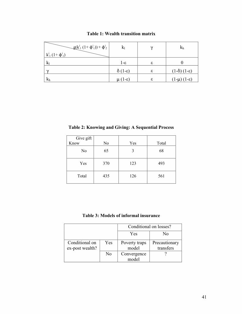
41

Table 1: Wealth transition matrix

g(ki1 (1+ Ni

1)) + Ni2

ki1 (1+ Ni

1)

kl ( kh

kl 1-ε ε 0

( * (1-ε) ε (1-*) (1-ε)

kh : (1-ε) ε (1-:) (1-ε)

Table 2: Knowing and Giving: A Sequential Process

Give gift Know

No

Yes

Total

No 65 3 68

Yes 370 123 493

Total 435 126 561

Table 3: Models of informal insurance

Conditional on losses? Yes No

Yes Poverty traps model

Precautionary transfers

Conditional on ex-post wealth?

No Convergence model

?

42

Table 4: Variable definitions and descriptive statistics

Variable Description Mean (std dev)

Distance Absolute value of the distance between i and j, in km

37.07 (55.78)

Same clan Dummy variable, equal to 1 if both i and j belong to the same clan 0.19 (0.39)

Male, male Dummy variable, equal to 1 if both i and j are male

0.41 (0.49)

Male, female Dummy variable, equal to 1 if i is male and j is female

0.24 (0.43)

Female, male Dummy variable, equal to 1 if i is female and j is male

0.22 (0.41)

Older Absolute value of the age difference between i and j if i is older, 0 otherwise 8.48 (12.92)

Younger Absolute value of the age difference between i and j if i is younger, 0 otherwise 8.18 (12.91)

More land Absolute value of the difference in land between i and j if i has more land than j, 0 otherwise

0.39 (1.27)

Less land Absolute value of the difference in land between i and j if i has less land than j, 0 otherwise

0.37 (1.11)

More cattle Absolute value of the difference in cattle between i and j if i has more cattle than j, 0 otherwise

5.53 (13.61)

Less cattle Absolute value of the difference in cattle between i and j if i has less cattle than j, 0 otherwise

5.24 (12.87)

Bigger family Absolute value of the difference in family size between i and j if i has a bigger family than j, 0 otherwise

1.59 (2.40)

Smaller family Absolute value of the difference in family size between i and j if i has a smaller family than j, 0 otherwise

1.66 (2.50)

Match has no cattle Dummy variable, equal to 1 if j has no cattle in September 2003 0.15 (0.36)

E1: poor Dummy variable, equal to 1 if j has more than 0 cattle but less than 5 cattle in September 2003

0.15 (0.36)

E2: intermediate herd size, below threshold

Dummy variable, equal to 1 if j has more than 4 but less than 15 cattle in September 2003 0.54 (0.50)

E3: intermediate herd size, above threshold

Dummy variable, equal to 1 if j has more than 14 but less than 40 cattle in September 2003 0.12 (0.33)

E4: wealthy Dummy variable, equal to 1 if j has more than 39 cattle in September 2003 0.03 (0.16)

Lj: herd loss Dummy variable, equal to 1 if j’s herd diminished between September 2000 and September 2003

0.21 (0.40)

Family size Number of people in the household

6.00 (3.15)

Herd size Number of cattle in September 2003

10.79 (14.75)

Expected wealth Probability that the match will have a herd bigger than 30 cattle, 10 years after having received a gift of one cattle, given current (2003) herd size.

0.065 (0.101)

Expected gains Difference in match’s expected herd size, after 10 years, conditional on receiving a gift of one cattle, given current (2003) herd size

1.063 (0.327)

Dida Hara Dummy variable, equal to 1 if the respondent lives in Dida Hara 0.258 (0.438)

Dillo Dummy variable, equal to 1 if the respondent lives in Dillo 0.258 (0.438)

43

Qorate Dummy variable, equal to 1 if the respondent lives in Qorate 0.261 (0.439)

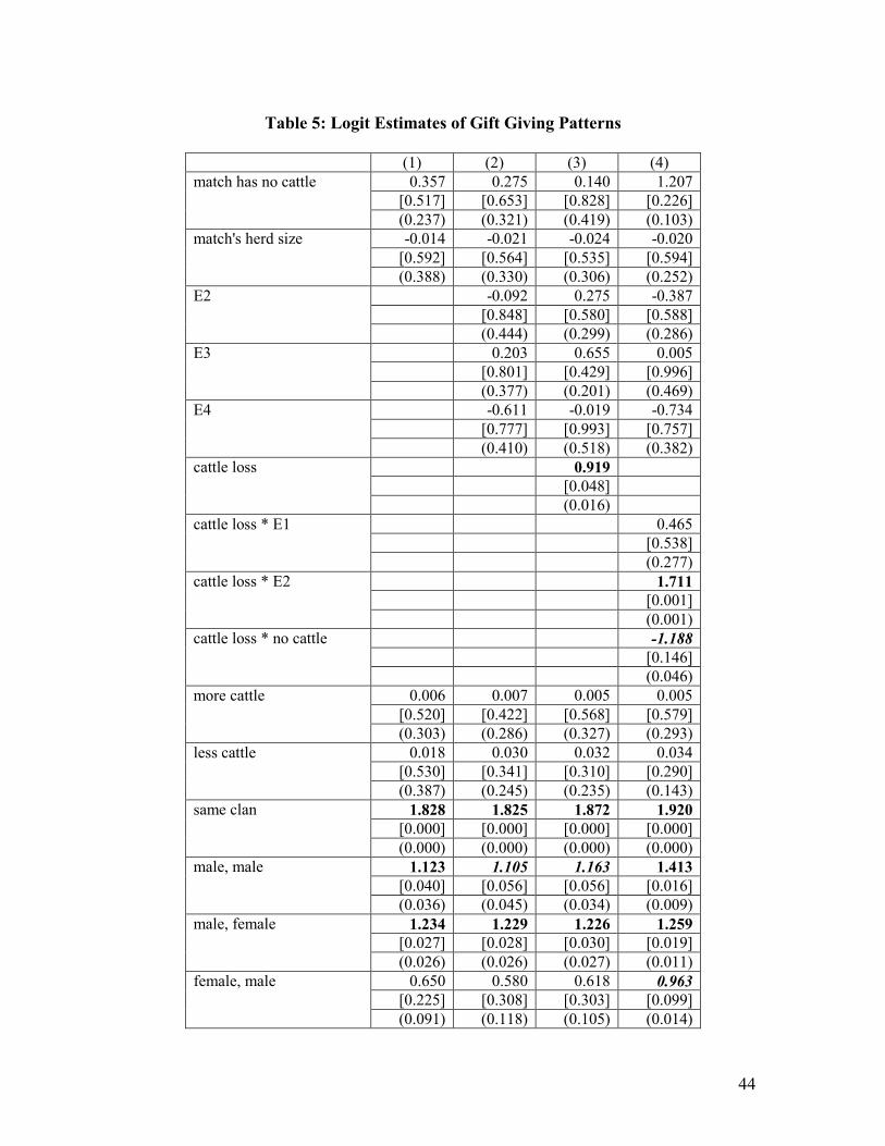
44

Table 5: Logit Estimates of Gift Giving Patterns

(1) (2) (3) (4) 0.357 0.275 0.140 1.207

[0.517] [0.653] [0.828] [0.226] match has no cattle

(0.237) (0.321) (0.419) (0.103) -0.014 -0.021 -0.024 -0.020

[0.592] [0.564] [0.535] [0.594] match's herd size

(0.388) (0.330) (0.306) (0.252) -0.092 0.275 -0.387

[0.848] [0.580] [0.588] E2

(0.444) (0.299) (0.286) 0.203 0.655 0.005

[0.801] [0.429] [0.996] E3

(0.377) (0.201) (0.469) -0.611 -0.019 -0.734

[0.777] [0.993] [0.757] E4

(0.410) (0.518) (0.382) 0.919

[0.048] cattle loss

(0.016) 0.465

[0.538] cattle loss * E1

(0.277) 1.711

[0.001] cattle loss * E2

(0.001) -1.188

[0.146] cattle loss * no cattle

(0.046) 0.006 0.007 0.005 0.005

[0.520] [0.422] [0.568] [0.579] more cattle

(0.303) (0.286) (0.327) (0.293) 0.018 0.030 0.032 0.034

[0.530] [0.341] [0.310] [0.290] less cattle

(0.387) (0.245) (0.235) (0.143) 1.828 1.825 1.872 1.920

[0.000] [0.000] [0.000] [0.000] same clan

(0.000) (0.000) (0.000) (0.000) 1.123 1.105 1.163 1.413

[0.040] [0.056] [0.056] [0.016] male, male

(0.036) (0.045) (0.034) (0.009) 1.234 1.229 1.226 1.259

[0.027] [0.028] [0.030] [0.019] male, female

(0.026) (0.026) (0.027) (0.011) 0.650 0.580 0.618 0.963

[0.225] [0.308] [0.303] [0.099] female, male

(0.091) (0.118) (0.105) (0.014)

45

Observations 493 493 493 493 Number of clusters 115 115 115 115 Log pseudolikelihood -211.19 -210.60 -208.03 -204.29 Pseudo R-squared 0.237 0.240 0.249 0.262 Adjusted count R-squared 0.293 0.285 0.285 0.341

Values within brackets are robust p-values. Values within parentheses are QAP-corrected p-values. Values in Bold are statistically significant at the 5% significance level or lower. Values in Bold are statistically significant at the 5% significance level or lower when p-values are obtained through the QAP. Distance, differences in age, land owned, family size, and respondent’s age and family size, together with village-specific dummy variables and a constant were included in the estimation but are not reported.

46

Table 6: Logit Estimates of Gift Giving Patterns: The effect of herder ability

(1) (2) (3) Coefficient Bootstrapped

standard errors Coefficient Bootstrapped

standard errors Coefficient Bootstrapped

standard errors Low 1.137 1.638 0.376 0.490 1.334 3.767 Medium 2.542 1.695 0.435 0.347 2.616 3.710 E2 * low 1.372 1.679 -0.248 0.717 E2 * medium -1.145 1.777 1.528 0.941 E2 *high 1.607 2.353 2.720 3.713 cattle loss * E2 * low dropped* cattle loss * E2 * medium 2.856 1.123 cattle loss * E2 * high 2.500 0.925 Note: Bootstrapped standard errors obtained using 200 replicates. All the covariates present in table 5, column 4, were included, but are not reported. Variables in bold are statistically significant at the 5% significance level or lower. * In the model presented under column (1), the variable “cattle loss * E2 * low” predicts failure perfectly – the variable was dropped and 8 observations were not used.

47

Table 7: Logit Estimates of Gift Giving Patterns: Expected wealth vs. Expected gains

(1) (2) (3) (4) (5)

-0.669 -0.865 -0.501 (1.705) (1.683) (1.764)

Expected wealth

[3.353] [2.381] [2.419] 0.139 0.229 0.353 (0.569) (0.580) (0.624)

Expected gains

[0.644] [0.688] [0.768] 21.868 -7.995 (8.554) (13.058)

Loss * Expected wealth

[11.013] [18.675] 1.555 1.849 (0.462) (0.652)

Loss * expected gains

[0.547] [0.898] Observations 484 484 484 484 484

Note: The values within parenthesis are robust standard errors and the values within brackets are bootstrapped standard errors, obtained using 200 replicates. All the covariates present in Table 5, column 4 (except those expressing herd’s position with respect to the different equilibria and their interactions) were included in the regression but are not reported. Values in Bold are statistically significant at the 5% significance level or lower when considering bootstrapped standard errors.

48

Table 8: Logit estimates of Gift-giving patterns: Additional explanations

(1) (2) Match has no cattle 0.347 2.130 [0.906] [0.417] Match’s herd size -0.029 -0.013 [0.480] [0.730] E1 0.775 0.814 [0.767] [0.739] E2 0.482 0.568 [0.837] [0.800] E3 0.743 0.919 [0.704] [0.622] Loss * match has no cattle 0.500 -1.143 [0.734] [0.221] Loss * E1 0.379 0.498 [0.625] [0.547] Loss * E2 2.100 1.663 [0.000] [0.001] Negative correlation -0.273 [0.736] Positive correlation 0.886 [0.222] Number of brothers -0.077 [0.761] Number of brothers squared 0.020 [0.515] Observations 436 452 Number of respondents 107.000 104.000 Log pseudolikelihood -182.705 -190.751 Pseudo R-squared 0.265 0.274 Adjusted count R-squared 0.339 0.364 Note: robust p-values within brackets. Values in Bold are significant at the 5%level of significance or smaller. All the covariates present in Table 5, column 4 were included in the regression but are not reported.

49

Table 9: Logit Estimates of Social Acquaintance Networks

Know Robust p-values

QAP corrected p-values

no cattle since 2000 -1.106 0.025 0.070 E1 since 2000 -0.145 0.736 0.392 E2 since 2000 -0.127 0.639 0.379 E3 since 2000 -0.581 0.558 0.485 E4 since 2000 -1.297 0.287 0.284 cattle loss since 2000 0.203 0.466 0.356 More cattle -0.014 0.009 0.096 less cattle 0.040 0.001 0.043 Distance -0.007 0.323 0.201 Same clan 0.743 0.015 0.033 Male, male 0.684 0.081 0.118 Male, female 0.177 0.671 0.359 female, male 0.618 0.084 0.121 Older -0.026 0.013 0.005 Younger -0.000 0.971 0.515 more land 0.143 0.215 0.193 less land 0.482 0.001 0.013 bigger family 0.042 0.499 0.264 smaller family -0.097 0.088 0.111 Observations 745 Number of respondents 85 Log pseudolikelihood -256.124 Pseudo R-squared 0.229 Adjusted count R-squared 0.041

Note: Values in Bold are statistically significant at the 5% level of significance or lower. Values in Bold italics remain statistically significant at the 5% level of significance or lower for p-values obtained through QAP. Village dummies and a constant were included in the estimation but are not reported here. Being from Qorate predicts being known perfectly – the variable was dropped and 300 observations were not used.

Documents

Informal insurance in the presence of poverty traps: Evidence