Embed Size (px)
Citation preview
IJMS 17 (2), 73–104 (2010)
INFLATION IN MALAYSIA
WONG HOCK TSENSchool of Business and Economics
Universiti Malaysia Sabah
Abstract
This study examines the determination of infl ation in Malaysia. The results of the generalised forecast error variance decomposition show that real import price change is the most important factor in the determination of infl ation. The impact of real oil price change on infl ation is marginal. An increase in real oil price has a more signifi cant impact on infl ation than a decrease in real oil price. The results of the generalised impulse response function show the impact of variables examined on infl ation is relatively short. There is evidence that real oil price change Granger causes infl ation.
Keywords: Infl ation; Malaysia; cointegration; generalised forecast error variance decomposition; generalised impulse response function.
Abstrak
Kajian ini menguji penentuan infl asi di Malaysia. Keputusan dekomposisi varian ralat ramalan umum menunjukkan bahawa perubahan harga import benar adalah faktor terpenting dalam penentuan infl asi di Malaysia. Impak perubahan harga minyak benar ke atas infl asi adalah marginal. Kenaikan dalam harga minyak benar mempunyai impak yang lebih signifi kan ke atas infl asi berbanding dengan kejatuhan dalam harga minyak benar. Keputusan fungsi tindak balas impuls umum menunjukkan impak pemboleh ubah yang diuji ke atas infl asi secara relatifnya adalah pendek. Terdapat bukti bahawa perubahan harga minyak benar menjadi penyebab Granger infl asi.
Kata Kunci: Infl asi; Malaysia; kointegrasi; dekomposisi varian ralat ramalan umum; fungsi tindak balas impuls umum.
Introduction
Malaysia achieved a relatively high and rapid economic growth over the past decades. In the 19701979 period, the average economic
http
://ijm
s.uu
m.e
du.m
y
74 IJMS 17 (2), 47–72 (2010)
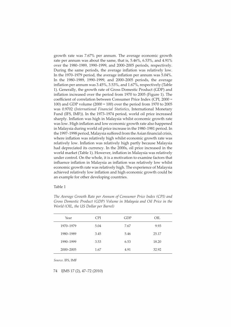
growth rate was 7.67% per annum. The average economic growth rate per annum was about the same, that is, 5.46%, 6.53%, and 4.91% over the 1980–1989, 1990–1999, and 2000–2005 periods, respectively. During the same periods, the average infl ation was relatively low. In the 1970–1979 period, the average infl ation per annum was 5.04%. In the 1980–1989, 1990–1999, and 2000–2005 periods, the average infl ation per annum was 3.45%, 3.53%, and 1.67%, respectively (Table 1). Generally, the growth rate of Gross Domestic Product (GDP) and infl ation increased over the period from 1970 to 2005 (Figure 1). The coeffi cient of correlation between Consumer Price Index (CPI, 2000 = 100) and GDP volume (2000 = 100) over the period from 1970 to 2005 was 0.9702 (International Financial Statistics, International Monetary Fund (IFS, IMF)). In the 1973–1974 period, world oil price increased sharply. Infl ation was high in Malaysia whilst economic growth rate was low. High infl ation and low economic growth rate also happened in Malaysia during world oil price increase in the 1980–1981 period. In the 1997–1998 period, Malaysia suff ered from the Asian fi nancial crisis, where infl ation was relatively high whilst economic growth rate was relatively low. Infl ation was relatively high partly because Malaysia had depreciated its currency. In the 2000s, oil price increased in the world market (Table 1). However, infl ation in Malaysia was relatively under control. On the whole, it is a motivation to examine factors that infl uence infl ation in Malaysia as infl ation was relatively low whilst economic growth rate was relatively high. The experience of Malaysia achieved relatively low infl ation and high economic growth could be an example for other developing countries.
Table 1
The Average Growth Rate per Annum of Consumer Price Index (CPI) and Gross Domestic Product (GDP) Volume in Malaysia and Oil Price in the World (OIL, the US Dollar per Barrel)
Year CPI GDP OIL
1970–1979 5.04 7.67 9.93
1980–1989 3.45 5.46 25.17
1990–1999 3.53 6.53 18.20
2000–2005 1.67 4.91 32.92
Source. IFS, IMF
http
://ijm
s.uu
m.e
du.m
y
IJMS 17 (2), 73–104 (2010) 75
There are many factors that could cause infl ation in an economy. Cunado and De Gracia (2005) examined the impact of real oil price change on infl ation in six Asian countries using the Johansen (1988) cointegration method and Granger causality test. The main results were real oil price change has a signifi cant short-run impact on infl ation and more signifi cant when real oil price change is defi ned in domestic currency than in the United States dollar ($US). The impact of real oil price change on infl ation is diff erent across economies in Asia. The study examined only the impact of various measures of real oil price change on infl ation, but does not examined other factors that cause infl ation. Cheng and Tan (2002) examined infl ation in Malaysia using the Johansen (1988) cointegration method, impulse response function, variance decomposition of the Sims (1980) approach. The results showed that external factors such as exchange rate and the rest of infl ation in Association of Southeast Asian Nations (ASEAN) are relatively more important than domestic factors in explaining infl ation in Malaysia. However, the study did not examine the impact of real oil price, real import price, and fi nancial development on infl ation. In 1986, oil price decrease failed to stimulate economic growth. This leads to the hypothesis that there is existence of an asymmetric relationship between oil price change and economic growth (Cunado & De Gracia, 2005, pp. 77–78; Cologni & Manera, 2008, p. 5). The relationship between oil price change and infl ation could also be asymmetric.
Figure 1. Plots of the Natural Logarithm of Consumer Price Index (CPI, 2000 = 100) and the Natural Logarithm of Gross Domestic Product (GDP, 2000 = 100) Volume, 1970–2005.
Source. IFS, IMF
Source: IFS, IMF
0
20
40
60
80
100
120
140
70 74 78 82 86 90 94 98 2002
CPIGDP
http
://ijm
s.uu
m.e
du.m
y
76 IJMS 17 (2), 73–104 (2010)
Uncontrolled infl ation could have a signifi cant negative impact on other economic variables in an economy and thus it is important to identify the determination of infl ation. In world oil price shocks of 1974–1975 and 1978–1979, Malaysia experienced double digit infl ation and achieved low economic growth rate. An increase in oil price in the world market recently could result in low economic growth in Malaysia. An increase in oil price will lead to a decrease in aggregate supply because higher energy prices mean that fi rms purchase less energy. Thus the productivity of any given amount of capital and labour declines and potential output falls. The decline in factor productivity implies real wages will be lower (Cunado & De Gracia, 2005, p. 66). This study examined the determination of infl ation in Malaysia using time-series data. Malaysia is a net oil exporter. The impact of oil price on a net oil exporter could be diff erent from a net oil importer. Moreover, an oil price shock could have a diff erent impact on diff erent countries due to diff erent economy and tax structures (Cunado & De Gracia, 2005, p. 66). More specifi cally, this study estimated a vector of nine variables, namely infl ation, real GDP, real budget defi cit, real money supply, real exchange rate, real interest rate, real import price, fi nancial development, and real oil price. Thus this study adds to the literature of infl ation in Malaysia by examining the impact of real import price, fi nancial development, and oil price on infl ation. The vector is estimated over the full sample, that is, from 1975QI to 2001QIV and a sub-sample, that is, from 1975QI to 1996QIV to exclude the Asian fi nancial crisis, 19971998, in the estimation. The asymmetric impact of real oil price change on infl ation was also examined. The asymmetric relationship between oil price and macroeconomics variables has been investigated in many papers (Cunado & De Gracia, 2005; Cologni & Manera, 2008). The impact of oil price increase will retard the economy by more than oil price decrease. Thus it is also important to examine the asymmetry impact of oil price on infl ation.
Oil Price and Infl ation in Malaysia
Oil price plays an important role in the economy. It is a vital source of energy and an important raw material in many manufacturing processes (Chang & Wong, 2003, p. 1151). Moreover, oil is an important source of fuel for transportation. Thus demand for oil is inelastic, especially in the short run. In 1970, world oil price was $US1.79 per barrel. In the 1973–1974 period, the world experienced oil price shocks. World oil price increased from $US2.44 per barrel in 1972 to $US3.27 per barrel in 1973. In 1974, world oil price was $US11.50 per barrel.
http
://ijm
s.uu
m.e
du.m
y
IJMS 17 (2), 73–104 (2010) 77
In other words, world oil price increased 33.90% in 1973 and 251.60% in 1974. As a result, infl ation in Malaysia increased 10.56% in 1973 and 17.33% in 1974. In 1979, the world experienced another oil price shock. World oil price increased from $US12.78 per barrel in 1978 to $US29.83 per barrel in 1979 or, increased 133.45%. Nonetheless, infl ation in Malaysia was relatively low at 3.65%. However, infl ation was high two years later, that is, 6.67% in 1980 and 9.70% in 1981. In the 19801981 period, the infl ation rates in Malaysia were relatively low when comparing to infl ation rates in the 1973–1974 period (IFS, IMF). The fi rst world oil price shocks had a more signifi cant impact on infl ation in Malaysia than the second world oil price shock.
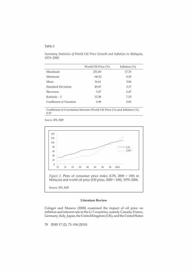
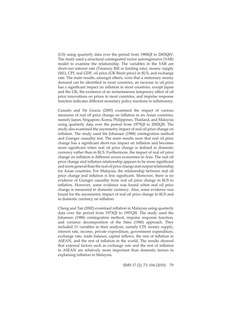
In the 19811986 period, the world experienced negative growth rates in oil price. Besides, in the 19851987 period, Malaysia experienced economic recession and infl ation rates were low, less than 1% in the period. In 1998, world oil price decreased 32.14%. However, infl ation was relatively high at 5.27 in Malaysia. The relatively high infl ation was the result of eff ect of the Asian fi nancial crisis. In order to check high imported infl ation, Malaysia fi xed its currency against $US at Malaysian ringgit 3.80 per $US on 2 September 1998. This move had promoted economic stability and restored public confi dence toward the fi nancial market in Malaysia Ministry of Finance, (MOF, 1999, p. 17). This move also helped to curve imported infl ation. In 1999 and 2000, world oil price increased to 37.53% and 57.02%, respectively. Nevertheless, infl ation rates were under control in Malaysia at 2.74% and 1.53% respectively. In the 2003–2006 period, world oil price increased to two digit levels. Conversely, infl ation rates in Malaysia were 1.06% in 2003, 1.45% in 2004, 2.96% in 2005, and 3.61% in 2006. In 2006, world oil price was $US64.27 per barrel. In 2008, the oil price was more than $US100 per barrel (IFS, IMF; Figure 2). On 21 July 2005, Malaysia fl oated its currency against $US and let the value of the currency be determined by market forces. The stronger Malaysian ringgit was supported by strong trade performance, sustained capital fl ows, and positive economic prospects. A strong currency helped to reduce infl ation through cheaper imports of goods and services (MOF, 2006, p. 2). Table 2 provides summary statistics of world oil price growth ($US) and infl ation in Malaysia. In the 1970-2006 period, world oil price increased from the lowest at $US1.79 per barrel in 1970 to the highest at $US64.27 per barrel in 2006. Generally, oil price increased over time. Infl ation ranged from the lowest rate at 0.29% to the highest rate at 17.33%. The coeffi cient of correlation between world oil price growth and infl ation in Malaysia was 0.57 over the period from 1970 to 2006. Thus there is strong relationship between these two variables.
http
://ijm
s.uu
m.e
du.m
y
78 IJMS 17 (2), 73–104 (2010)
Table 2
Summary Statistics of World Oil Price Growth and Infl ation in Malaysia, 19702006
World Oil Price (%) Infl ation (%)
Maximum 251.60 17.33
Minimum –48.22 0.29
Mean 16.61 3.84
Standard Deviation 49.47 3.17
Skewness 3.27 2.47
Kurtosis – 3 12.58 7.53
Coeffi cient of Variation 2.98 0.83
Coeffi cient of Correlation between World Oil Price (%) and Infl ation (%) 0.57
Source. IFS, IMF
Figure 2. Plots of consumer price index (CPI, 2000 = 100) in Malaysia and world oil price (Oil price, 2000 = 100), 1970–2006. Source. IFS, IMF
Literature Review
Cologni and Manera (2008) examined the impact of oil price on infl ation and interest rate in the G-7 countries, namely Canada, France, Germany, Italy, Japan, the United Kingdom (UK), and the United States
Source: IFS, IMF
0
20
40
60
80
100
120
140
70 74 78 82 86 90 94 98 2002
CPIGDP
http
://ijm
s.uu
m.e
du.m
y
IJMS 17 (2), 73–104 (2010) 79
(US) using quarterly data over the period from 1980QI to 2003QIV. The study used a structural cointegrated vector autoregressive (VAR) model to examine the relationship. The variables in the VAR are short-run interest rate (Treasury Bill or lending rate), money supply (M1), CPI, real GDP, oil price (UK Brent price) in $US, and exchange rate. The main results, amongst others, were that a stationary money demand can be identifi ed in most countries, an increase in oil price has a signifi cant impact on infl ation in most countries, except Japan and the UK, the existence of an instantaneous temporary eff ect of oil price innovations on prices in most countries, and impulse response function indicates diff erent monetary policy reactions to infl ationary.
Cunado and De Gracia (2005) examined the impact of various measures of real oil price change on infl ation in six Asian countries, namely Japan, Singapore, Korea, Philippines, Thailand, and Malaysia using quarterly data over the period from 1975QI to 2002QII. The study also examined the asymmetry impact of real oil price change on infl ation. The study used the Johansen (1988) cointegration method and Granger causality test. The main results were that real oil price change has a signifi cant short-run impact on infl ation and becomes more signifi cant when real oil price change is defi ned in domestic currency rather than in $US. Furthermore, the impact of real oil price change on infl ation is diff erent across economies in Asia. The real oil price change and infl ation relationship appears to be more signifi cant and more general than the real oil price change and output relationship for Asian countries. For Malaysia, the relationship between real oil price change and infl ation is less signifi cant. Moreover, there is no evidence of Granger causality from real oil price change in $US to infl ation. However, some evidence was found when real oil price change is measured in domestic currency. Also, some evidence was found for the asymmetric impact of real oil price change in $US and in domestic currency on infl ation.
Cheng and Tan (2002) examined infl ation in Malaysia using quarterly data over the period from 1973QI to 1997QII. The study used the Johansen (1988) cointegration method, impulse response function, and variance decomposition of the Sims (1980) approach. They included 11 variables in their analysis, namely CPI, money supply, interest rate, income, private expenditure, government expenditure, exchange rate, trade balance, capital infl ows, the rest of infl ation in ASEAN, and the rest of infl ation in the world. The results showed that external factors such as exchange rate and the rest of infl ation in ASEAN are relatively more important than domestic factors in explaining infl ation in Malaysia.
http
://ijm
s.uu
m.e
du.m
y
80 IJMS 17 (2), 73–104 (2010)
Mansor (2003) examined the impact of the US macroeconomic variables on the Malaysian economy using monthly data over the period from 1977 to 1988. The study also used the Johansen (1988) cointegration method, impulse response function, and variance decomposition of the Sims (1980) approach. The variables in the VAR are real industrial production, CPI, three month Treasury Bill rates, and money supply (M2) of Malaysia, and real industrial production, federal fund rates, CPI, and exchange rate of the US. The results showed that the foreign price level and real industrial production do infl uence exchange rate, which in turn infl uences domestic variables including real industrial production, price level, and money supply. More specifi cally, an increase in the US real industrial production or monetary policy has an impact on the Malaysian real industrial production. An increase in money supply in Malaysia or the US lagged infl ation will lead to an increase in infl ation in Malaysia. The study emphasised the importance of exchange rate stability for the Malaysian economy.
Methodology and Data
The Dickey and Fuller (1979) (DF), and Phillips and Perron (1988) (PP) unit root test statistics are used mainly to examine the stationarity of the data. The Johansen (1988) cointegration method is used to examine the long-run relationship among variables in a system. This study estimated a vector of nine variables, namely infl ation (Pd,t), real GDP (Yt), real budget defi cit (BDt), real money supply (MSt), real exchange rate (ERt), real interest rate (Rt), real import price (Pm,t), fi nancial development (FDt), and real oil price (Po,t). An increase in real GDP, real budget defi cit, or real money supply will lead to an increase in aggregate demand. These variables are examined mainly because they are argued to be important factors in the determination of infl ation (Cheng & Tan, 2002; Mansor, 2003; Cunado & De Gracia, 2005; Cologni & Manera, 2008). An increase in aggregate demand will lead to an increase in infl ation (Romer, 2001). The coeffi cients of real GDP, real budget defi cit, and real money supply are expected to be positive.
An increase in fi nancial development will lead to an increase in aggregate demand and thus an increase in economic growth. Also, an increase in fi nancial development will lead to an increase in aggregate supply and thus an increase in economic growth. Aggregate demand and aggregate supply can move at the same time. However, this does not imply that they will change at the same proportion. As a result, price level may not be the same. Cointegration means that two or
http
://ijm
s.uu
m.e
du.m
y
IJMS 17 (2), 73–104 (2010) 81
more series are themselves non-stationary but a linear combination of them is stationary. More specifi cally, a (n × 1) vector time series yt is said to be cointegrated if each of the series is nonstationary with a unit root and some linear combination of the series a’y is stationary for some nonzero (n × 1) vector a (Engle & Granger, 1987). In other words, the series are cointegrated partly because the vector a is nonzero. A sound fi nancial system is important for economic growth as fi nancial system facilitates the allocation of resources over time and space (King & Levine, 1993; Levine, 1997; Ang, 2008). An increase in economic growth will lead to an increased aggregate demand, which in turn increases infl ation. The coeffi cient of fi nancial development is expected to be positive.
An increase in real import price or real oil price will lead to an increase in costs of production or prices of goods. Thus infl ation will increase (Cunado & De Gracia, 2005; Cologni & Manera, 2008). The coeffi cients of real import price and real oil price are expected to be positive. An increase in real interest rate will lead to a decrease in investment and thus aggregate demand will decrease. This will lead to a decrease in economic growth and infl ation. Moreover, an increase in real interest rate will lead to an increase in infl ation, that is an increase in real interest rate could lead to an increase in cost of production and thus infl ation will increase. Linnemann (2005, p. 308) used a new Keynesian sticky price business cycle model to show that an increase in interest rate will lead to an increase in infl ation. More specifi cally, a higher interest rate with a balanced government budget implements a higher tax rate which implies higher interest rate payments on debt would discourage current labour supply for intertemporal substitution reasons. Thus there will be upward pressure on wages and infl ation. An increase in real interest rate will lead to an increase or a decrease in infl ation could be an empirical matt er. The coeffi cient of real interest rate is expected to be positive.
Conversely, an increase in real exchange rate, which implies a real appreciation in ringgit, will decrease trade balance if the elasticity of import demand is larger than the elasticity of export supply. On the other hand, an increase in real exchange rate will increase trade balance if the elasticity of import demand is smaller than the elasticity of export supply. In other words, the sum of the elasticity of import demand and the elasticity of export supply exceed unity, namely the Marshall-Lerner condition holds (Daniels & VanHoose, 2005, pp. 276277), an increase in real exchange rate will lead to a decrease in trade balance and economic growth. Thus infl ation will decrease. The coeffi cient of real exchange rate is expected to be negative.
http
://ijm
s.uu
m.e
du.m
y
82 IJMS 17 (2), 73–104 (2010)
The generalised forecast error variance decomposition and generalised impulse response function (Koop, Pesaran & Pott er, 1996; Pesaran & Shin, 1998) are used to examine the relationship of variables in a system. The generalised forecast error variance decomposition identifi es the proportion of forecast error variance in one variable caused by the innovations in other variables in a system. Therefore, the relative importance of a set of variables that aff ect a variance of another variable can be identifi ed. The generalised impulse response function traces the dynamic responses of a variable to innovations in other variables in a system. The generalised forecast error variance decomposition and generalised impulse response function (Koop, et al., 1996; Pesaran & Shin, 1998) may solve the orthogonalised problem of the forecast error variance decomposition and impulse response function of Sims (1980). The problem is that the latt er approaches are sensitive to the order of the variables in a VAR system.
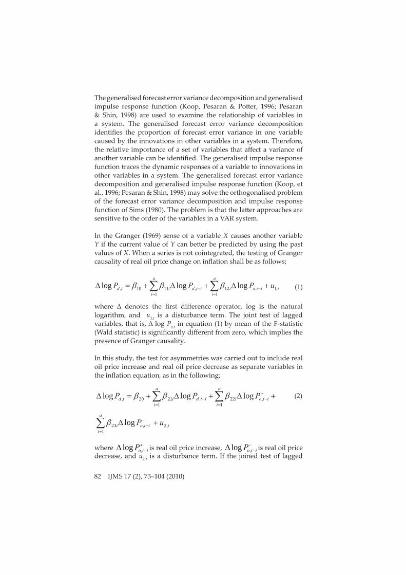
In the Granger (1969) sense of a variable X causes another variable Y if the current value of Y can bett er be predicted by using the past values of X. When a series is not cointegrated, the testing of Granger causality of real oil price change on infl ation shall be as follows;
(1)
where ∆ denotes the fi rst diff erence operator, log is the natural logarithm, and u1,t is a disturbance term. The joint test of lagged variables, that is, ∆ log Po,t in equation (1) by mean of the F-statistic (Wald statistic) is signifi cantly diff erent from zero, which implies the presence of Granger causality.
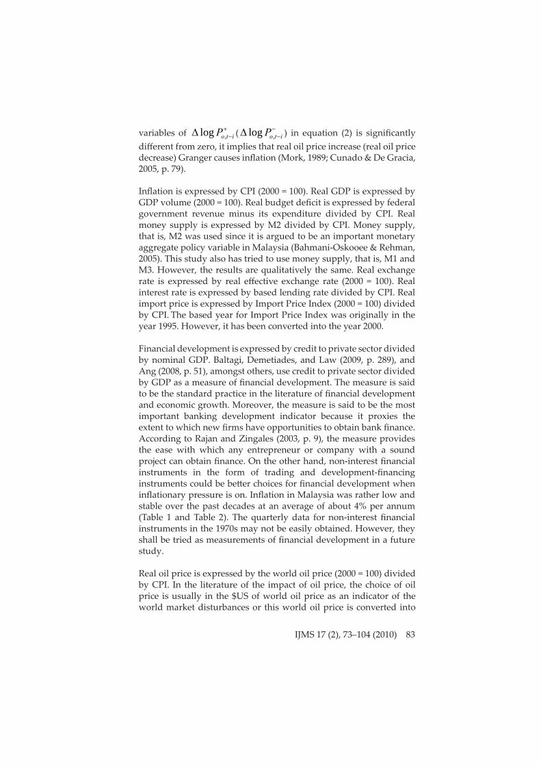
In this study, the test for asymmetries was carried out to include real oil price increase and real oil price decrease as separate variables in the infl ation equation, as in the following;
(2)
where itoP ,log is real oil price increase,
itoP ,log is real oil price decrease, and u2,t is a disturbance term. If the joined test of lagged
a
iitoi P
1,23 log tu ,2
a
iitoi
a
iitditd PPP
1,22
1,2120, logloglog
a
ititoi
a
iitditd uPPP
1,1,12
1,1110, logloglog
http
://ijm
s.uu
m.e
du.m
y
IJMS 17 (2), 73–104 (2010) 83
variables of itoP ,log (
itoP ,log ) in equation (2) is signifi cantly diff erent from zero, it implies that real oil price increase (real oil price decrease) Granger causes infl ation (Mork, 1989; Cunado & De Gracia, 2005, p. 79).
Infl ation is expressed by CPI (2000 = 100). Real GDP is expressed by GDP volume (2000 = 100). Real budget defi cit is expressed by federal government revenue minus its expenditure divided by CPI. Real money supply is expressed by M2 divided by CPI. Money supply, that is, M2 was used since it is argued to be an important monetary aggregate policy variable in Malaysia (Bahmani-Oskooee & Rehman, 2005). This study also has tried to use money supply, that is, M1 and M3. However, the results are qualitatively the same. Real exchange rate is expressed by real eff ective exchange rate (2000 = 100). Real interest rate is expressed by based lending rate divided by CPI. Real import price is expressed by Import Price Index (2000 = 100) divided by CPI. The based year for Import Price Index was originally in the year 1995. However, it has been converted into the year 2000.
Financial development is expressed by credit to private sector divided by nominal GDP. Baltagi, Demetiades, and Law (2009, p. 289), and Ang (2008, p. 51), amongst others, use credit to private sector divided by GDP as a measure of fi nancial development. The measure is said to be the standard practice in the literature of fi nancial development and economic growth. Moreover, the measure is said to be the most important banking development indicator because it proxies the extent to which new fi rms have opportunities to obtain bank fi nance. According to Rajan and Zingales (2003, p. 9), the measure provides the ease with which any entrepreneur or company with a sound project can obtain fi nance. On the other hand, non-interest fi nancial instruments in the form of trading and development-fi nancing instruments could be bett er choices for fi nancial development when infl ationary pressure is on. Infl ation in Malaysia was rather low and stable over the past decades at an average of about 4% per annum (Table 1 and Table 2). The quarterly data for non-interest fi nancial instruments in the 1970s may not be easily obtained. However, they shall be tried as measurements of fi nancial development in a future study.
Real oil price is expressed by the world oil price (2000 = 100) divided by CPI. In the literature of the impact of oil price, the choice of oil price is usually in the $US of world oil price as an indicator of the world market disturbances or this world oil price is converted into
http
://ijm
s.uu
m.e
du.m
y
84 IJMS 17 (2), 73–104 (2010)
respective currency by means of the market exchange rate. The diff erence between the two variables is that only the second one takes into account the diff erences in the oil price that a country faces due to its exchange rate fl uctuations or its infl ation levels (Cologni & Manera, 2008). This index is used as its movements with other oil price indexes, namely the United Arab Emirates oil price (Dubai), the British oil price (Brent), and West Texas intermediate oil price (Texas), were about the same. Generally, the coeffi cient of correlation of this index with other index was 0.99 over the period from 1960 to 2006. Thus this index is expected to give a good indicate of the movements of oil price in the world.
CPI, GDP volume, real eff ective exchange rate, money supply (M2), nominal GDP (RM millions), credit to private sector (RM millions), and the world oil price (2000 = 100) were obtained from IFS, IMF. Based lending rate, federal government revenue (RM millions), and federal government expenditure (RM millions) were obtained from Economic Report, Ministry of Finance of Malaysia. Import Price Index (2000 = 100) was obtained from the World Bank Table, the World Bank. For real GDP, real budget defi cit, and import price, the data were originally annually. The data have been converted into quarterly using the average of three quarters of an annual rate subsequently. For example, the data for 1975QIII is an average of the data for 1975QII, 1975QIII, and 1975QIV.
A change in real oil price is said to have asymmetric impact on infl ation (Cunado & De Gracia, 2005, pp. 77–78; Cologni & Manera, 2008, p. 5). The asymmetric impact of real oil price change is measured as: (i) real oil price increase is measured as toP ,log = max (0, toP ,log ) and (ii) real oil price decrease is measured as toP ,log = min (0, toP ,log ) (Cunado & De Gracia, 2005, pp. 69, 79). The samples are over the full sample, that is, from 1975QI to 2001QIV and a sub-sample, that is, from 1975QI to 1996QIV to exclude the Asian fi nancial crisis, 19971998 in the estimation, which could aff ect the estimation result. For estimation in full sample, a dummy variable is included as an additional explanatory variable to capture the Asian fi nancial crisis, that is, 1 for the period from 1997QI to 1998QIV and the rest are 0. The data are seasonality unadjusted and were transformed into the natural logarithm before estimation.
Empirical Results and Discussions
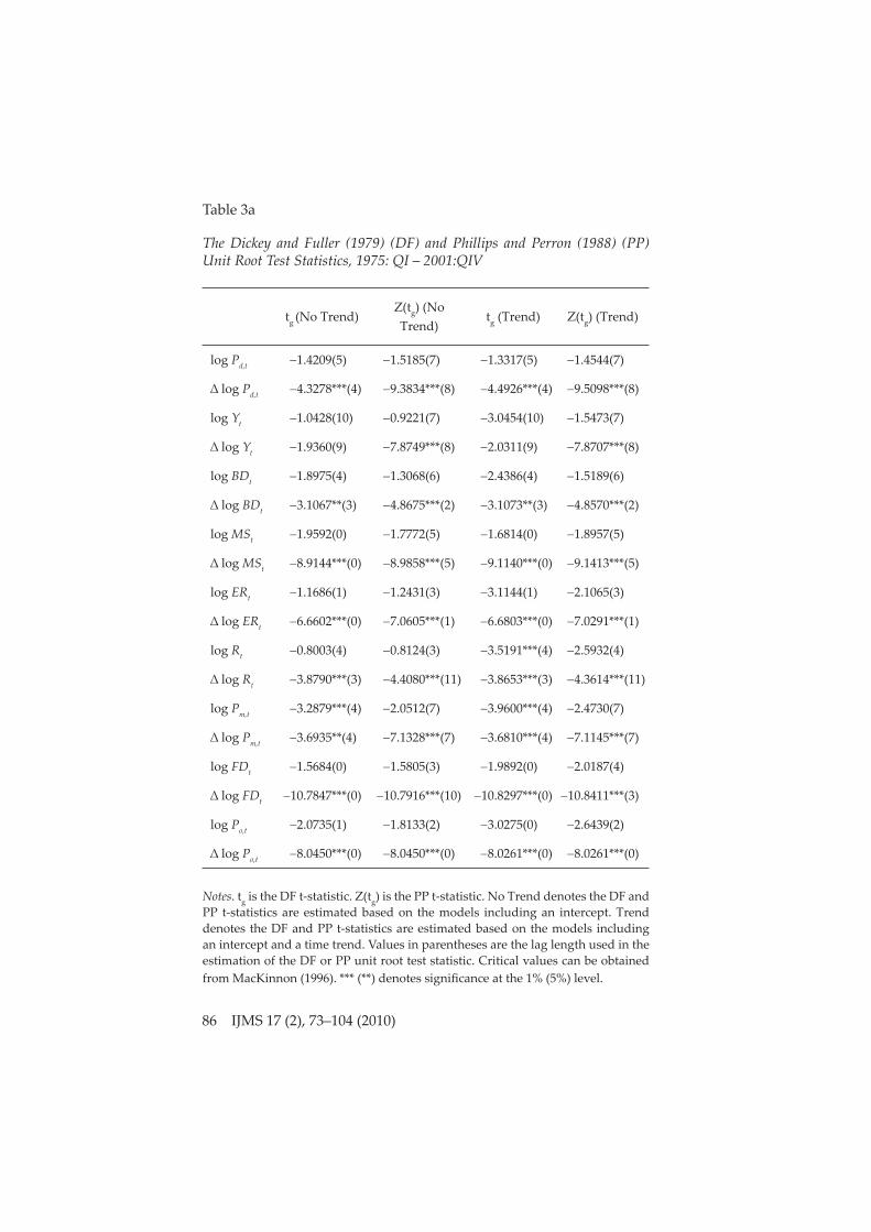
The DF and PP unit root test statistics are reported in Table 3a. The lag length used to estimate the DF unit root test statistics is based on
http
://ijm
s.uu
m.e
du.m
y
IJMS 17 (2), 73–104 (2010) 85
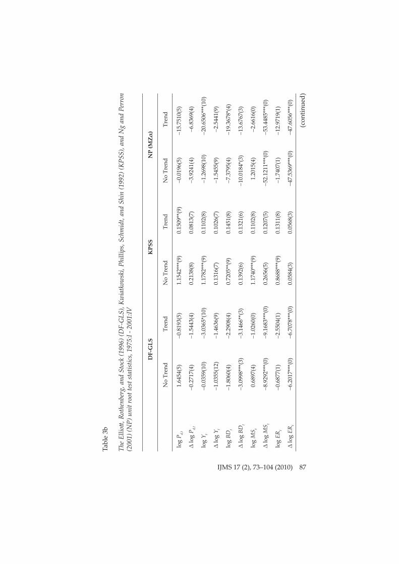
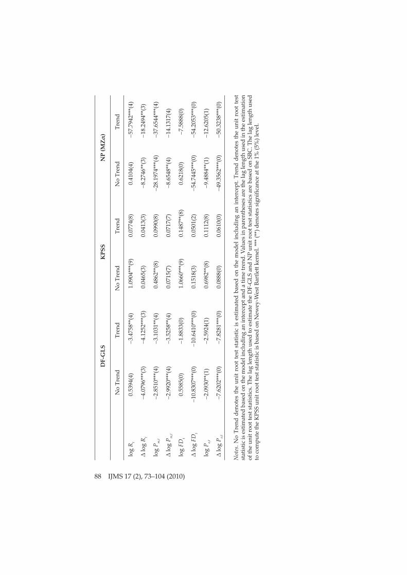
Schwarz Bayesian criterion (SBC). The lag length used to compute the PP unit root test statistics is based on Newey-West Bandwidth, with the maximum lag length set to 12. The results of the DF and PP unit root test statistics showed that all the variables, namely infl ation, real budget defi cit, real money supply, real exchange rate, real import price, fi nancial development, and real oil price, are non-stationary in level but becoming stationary after taking the fi rst diff erences, except real GDP, real interest rate, and real import price. For real GDP and real import price, the result of the DF unit root test statistic (no-trend or trend) showed no evidence of a unit root whilst the PP unit root test statistic (no-trend or trend) showed evidence of a unit root. For real interest rate, the result of the DF unit root test statistic (trend) showed no evidence of a unit root. Conversely, the DF unit root test statistic (no-trend) and PP unit root test statistic (no-trend or trend) showed evidence of a unit root. Nonetheless, it could be considered as a borderline case and thus it was treated as an I(1) series in this study. The results of the Elliott , Rothenberg, and Stock (1996), Kwiatkowski, Phillips, Schmidt, and Shin (1992), and Ng and Perron (2001) unit root test statistics are reported in Table 3b. Generally, all the variables examined could be treated as I(1) series.
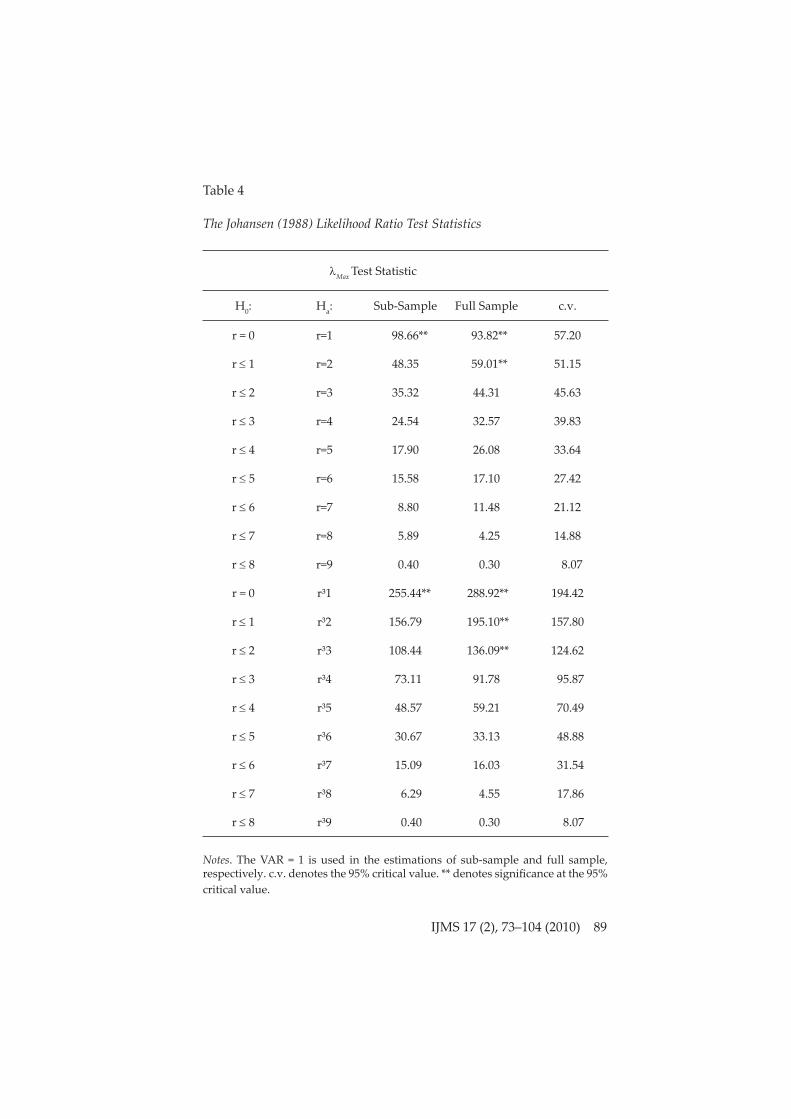
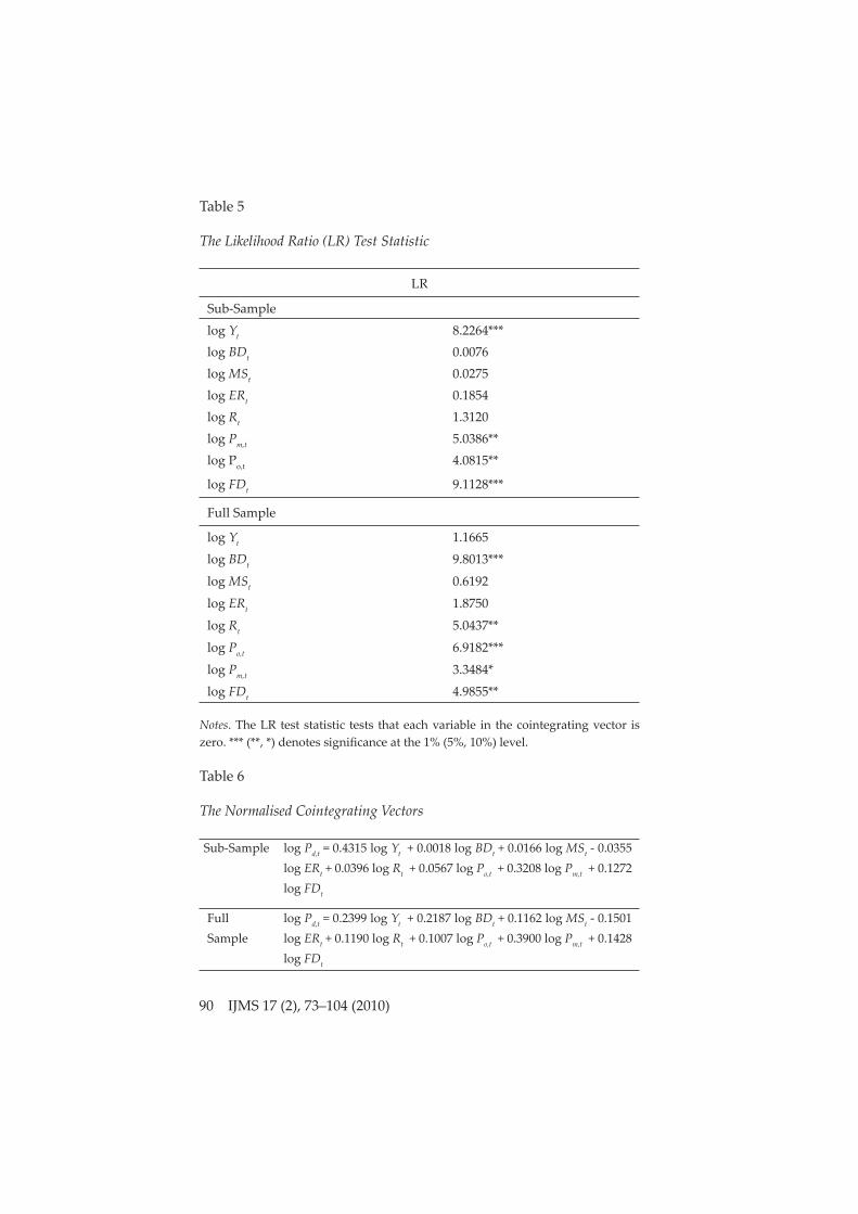
The results of the Johansen (1988) cointegration method are reported in Table 4. The results of the Max and Trace test statistics were computed with unrestricted intercepts and no trends. The lag length used in the estimations of the Max and Trace test statistics were based on SBC. For sub-sample, the results of the Max and Trace test statistics showed that there is one cointegrating vector. For the full sample, the result of the Max test statistic showed that there are two cointegrating vectors whilst the Trace test statistic showed that there are three cointegrating vectors. Thus the results of the Max and Trace test statistics showed that there is at least one cointegration vector. The likelihood ratio (LR) test statistic was used to test that each variable in the cointegrating vector is zero. The results of the LR test statistic are reported in Table 5. Generally, most of the variables were found important to be included in the estimation. The results of the normalised cointegrating vectors are reported in Table 6. On the whole, explanatory variables in the long-run equations were found to have the expected signs. An increase in real GDP, real budget defi cit, real money supply, real interest rate, real import price, fi nancial development, or real oil price will lead to an increase in infl ation. On the other hand, an increase in real exchange rate will lead to a decrease in infl ation. Moreover, the estimated coeffi cients of variables in the sub-sample and full sample are not much diff erent.
http
://ijm
s.uu
m.e
du.m
y
86 IJMS 17 (2), 73–104 (2010)
Table 3a
The Dickey and Fuller (1979) (DF) and Phillips and Perron (1988) (PP) Unit Root Test Statistics, 1975: QI – 2001:QIV
tg (No Trend)Z(tg) (No Trend)
tg (Trend) Z(tg) (Trend)
log Pd,t 1.4209(5) 1.5185(7) 1.3317(5) 1.4544(7)
∆ log Pd,t 4.3278***(4) 9.3834***(8) 4.4926***(4) 9.5098***(8)
log Yt 1.0428(10) 0.9221(7) 3.0454(10) 1.5473(7)
∆ log Yt 1.9360(9) 7.8749***(8) 2.0311(9) 7.8707***(8)
log BDt 1.8975(4) 1.3068(6) 2.4386(4) 1.5189(6)
∆ log BDt 3.1067**(3) 4.8675***(2) 3.1073**(3) 4.8570***(2)
log MSt 1.9592(0) 1.7772(5) 1.6814(0) 1.8957(5)
∆ log MSt 8.9144***(0) 8.9858***(5) 9.1140***(0) 9.1413***(5)
log ERt 1.1686(1) 1.2431(3) 3.1144(1) 2.1065(3)
∆ log ERt 6.6602***(0) 7.0605***(1) 6.6803***(0) 7.0291***(1)
log Rt 0.8003(4) 0.8124(3) 3.5191***(4) 2.5932(4)
∆ log Rt 3.8790***(3) 4.4080***(11) 3.8653***(3) 4.3614***(11)
log Pm,t 3.2879***(4) 2.0512(7) 3.9600***(4) 2.4730(7)
∆ log Pm,t 3.6935**(4) 7.1328***(7) 3.6810***(4) 7.1145***(7)
log FDt 1.5684(0) 1.5805(3) 1.9892(0) 2.0187(4)
∆ log FDt 10.7847***(0) 10.7916***(10) 10.8297***(0) 10.8411***(3)
log Po,t 2.0735(1) 1.8133(2) 3.0275(0) 2.6439(2)
∆ log Po,t 8.0450***(0) 8.0450***(0) 8.0261***(0) 8.0261***(0)
Notes. tg is the DF t-statistic. Z(tg) is the PP t-statistic. No Trend denotes the DF and PP t-statistics are estimated based on the models including an intercept. Trend denotes the DF and PP t-statistics are estimated based on the models including an intercept and a time trend. Values in parentheses are the lag length used in the estimation of the DF or PP unit root test statistic. Critical values can be obtained from MacKinnon (1996). *** (**) denotes signifi cance at the 1% (5%) level.
http
://ijm
s.uu
m.e
du.m
y
IJMS 17 (2), 73–104 (2010) 87
Tabl
e 3b
The
Elliott ,
Rot
henb
erg,
and
Sto
ck (1
996)
(DF-
GLS
), Kw
iatk
owsk
i, Ph
illip
s, Sc
hmid
t, an
d Sh
in (1
992)
(KPS
S), a
nd N
g an
d Pe
rron
(2
001)
(NP)
uni
t roo
t tes
t sta
tistic
s, 19
75:I
- 200
1:IV
DF-
GLS
KPS
SN
P (M
Zα)
No
Tren
dTr
end
No
Tren
dTr
end
No
Tren
dTr
end
log
P d,t
1.
6454
(5)
0.
8193
(5)
1.15
42**
*(9)
0.15
09**
(9)
0.
0196
(5)
1
5.75
10(5
)
∆ lo
g P d,
t
0.27
17(4
)
1.54
43(4
)0.
2138
(8)
0.08
13(7
)
3.92
41(4
)
6.83
69(4
)
log
Y t
0.03
59(1
0)
3.03
65*(
10)
1.17
82**
*(9)
0.11
02(8
)
1.26
98(1
0)2
0.65
06**
*(10
)
∆ lo
g Y t
1.
0355
(12)
1.
4636
(9)
0.13
16(7
)0.
1026
(7)
1.
5455
(9)
2.
5441
(9)
log
BDt
1.
8060
(4)
2.
2908
(4)
0.72
05**
(9)
0.14
51(8
)
7.37
95(4
)
1
9.36
78*(
4)
∆ lo
g BD
t
3.09
98**
*(3)
3.
1466
**(3
)0.
1392
(6)
0.13
21(6
)1
0.01
84*(
3)
1
3.67
67(3
)
log
MS t
0.
6897
(4)
1.
0260
(0)
1.17
40**
*(9)
0.11
02(8
)
1.20
15(4
)
2.66
16(0
)
∆ lo
g M
S t
8.92
92**
*(0)
9.
1683
***(
0)0.
2656
(5)
0.12
07(5
)5
2.12
11**
*(0)
5
3.44
85**
*(0)
log
ERt
0.
6877
(1)
2.
5504
(1)
0.86
88**
*(9)
0.13
11(8
)
1.74
07(1
)
1
2.97
19(1
)
∆ lo
g ER
t
6.20
17**
*(0)
6.
7078
***(
0)0.
0584
(3)
0.05
68(3
)4
7.53
69**
*(0)
4
7.60
56**
*(0)
(con
tinue
d)
http
://ijm
s.uu
m.e
du.m
y
88 IJMS 17 (2), 73–104 (2010)
DF-
GLS
KPS
SN
P (M
Zα)
No
Tren
dTr
end
No
Tren
dTr
end
No
Tren
dTr
end
log
R t
0.53
94(4
)
3.47
58**
(4)
1.09
04**
*(9)
0.07
74(8
)
0.41
04(4
) 5
7.79
42**
*(4)
∆ lo
g R t
4.
0796
***(
3)
4.12
52**
*(3)
0.04
65(3
)0.
0413
(3)
8.
2746
**(3
) 1
8.24
94**
(3)
log
P m,t
2.
8510
***(
4)
3.10
31**
(4)
0.48
62**
(8)
0.09
90(8
)2
8.19
74**
*(4)
3
7.65
44**
*(4)
∆ lo
g P m
,t
2.99
20**
*(4)
3.
5258
**(4
)0.
0715
(7)
0.07
17(7
)
8.65
48**
(4)
1
4.13
17(4
)
log
FDt
0.
5585
(0)
1.
8833
(0)
1.06
60**
*(9)
0.14
87**
(8)
0.
6218
(0)
7.
5888
(0)
∆ lo
g FD
t1
0.83
07**
*(0)
10.
6410
***(
0)0.
1518
(3)
0.05
01(2
)5
4.74
45**
*(0)
5
4.20
53**
*(0)
log
P o,t
2.
0930
**(1
)
2.59
24(1
)0.
6982
**(8
)0.
1112
(8)
9.
4884
**(1
)
1
2.62
05(1
)
∆ lo
g P o,
t
7.62
02**
*(0)
7.
8281
***(
0)0.
0888
(0)
0.06
10(0
)4
9.35
62**
*(0)
5
0.32
38**
*(0)
Not
es. N
o Tr
end
deno
tes
the
unit
root
test
sta
tistic
is e
stim
ated
bas
ed o
n th
e m
odel
incl
udin
g an
inte
rcep
t. Tr
end
deno
tes
the
unit
root
test
st
atis
tic is
est
imat
ed b
ased
on
the
mod
el in
clud
ing
an in
terc
ept a
nd a
tim
e tr
end.
Val
ues i
n pa
rent
hese
s are
the
lag
leng
th u
sed
in th
e es
timat
ion
of th
e un
it ro
ot te
st s
tatis
tics.
The
lag
leng
th u
sed
to e
stim
ate
the
DF-
GLS
and
NP
unit
root
test
sta
tistic
s ar
e ba
sed
on S
BC. T
he la
g le
ngth
use
d to
com
pute
the
KPS
S un
it ro
ot te
st s
tatis
tic is
bas
ed o
n N
ewey
-Wes
t Bar
tlett
kern
el. *
** (*
*) d
enot
es s
ignifi c
ance
at t
he 1
% (5
%) l
evel
.
http
://ijm
s.uu
m.e
du.m
y
IJMS 17 (2), 73–104 (2010) 89
Table 4
The Johansen (1988) Likelihood Ratio Test Statistics
Max Test Statistic
H0: Ha: Sub-Sample Full Sample c.v.
r = 0 r=1 98.66** 93.82** 57.20
r 1 r=2 48.35 59.01** 51.15
r 2 r=3 35.32 44.31 45.63
r 3 r=4 24.54 32.57 39.83
r 4 r=5 17.90 26.08 33.64
r 5 r=6 15.58 17.10 27.42
r 6 r=7 8.80 11.48 21.12
r 7 r=8 5.89 4.25 14.88
r 8 r=9 0.40 0.30 8.07
r = 0 r³1 255.44** 288.92** 194.42
r 1 r³2 156.79 195.10** 157.80
r 2 r³3 108.44 136.09** 124.62
r 3 r³4 73.11 91.78 95.87
r 4 r³5 48.57 59.21 70.49
r 5 r³6 30.67 33.13 48.88
r 6 r³7 15.09 16.03 31.54
r 7 r³8 6.29 4.55 17.86
r 8 r³9 0.40 0.30 8.07
Notes. The VAR = 1 is used in the estimations of sub-sample and full sample, respectively. c.v. denotes the 95% critical value. ** denotes signifi cance at the 95% critical value.
http
://ijm
s.uu
m.e
du.m
y
90 IJMS 17 (2), 73–104 (2010)
Table 5
The Likelihood Ratio (LR) Test Statistic
LR
Sub-Sample
log Yt 8.2264***log BDt 0.0076log MSt 0.0275log ERt 0.1854log Rt 1.3120log Pm,t 5.0386**log Po,t 4.0815**
log FDt 9.1128***
Full Sample
log Yt 1.1665
log BDt 9.8013***
log MSt 0.6192
log ERt 1.8750
log Rt 5.0437**
log Po,t 6.9182***
log Pm,t 3.3484*
log FDt 4.9855**
Notes. The LR test statistic tests that each variable in the cointegrating vector is zero. *** (**, *) denotes signifi cance at the 1% (5%, 10%) level.
Table 6
The Normalised Cointegrating Vectors
Sub-Sample log Pd,t = 0.4315 log Yt + 0.0018 log BDt + 0.0166 log MSt - 0.0355 log ERt + 0.0396 log Rt + 0.0567 log Po,t + 0.3208 log Pm,t + 0.1272 log FDt
Full Sample
log Pd,t = 0.2399 log Yt + 0.2187 log BDt + 0.1162 log MSt - 0.1501 log ERt + 0.1190 log Rt + 0.1007 log Po,t + 0.3900 log Pm,t + 0.1428 log FDt
http
://ijm
s.uu
m.e
du.m
y
IJMS 17 (2), 73–104 (2010) 91
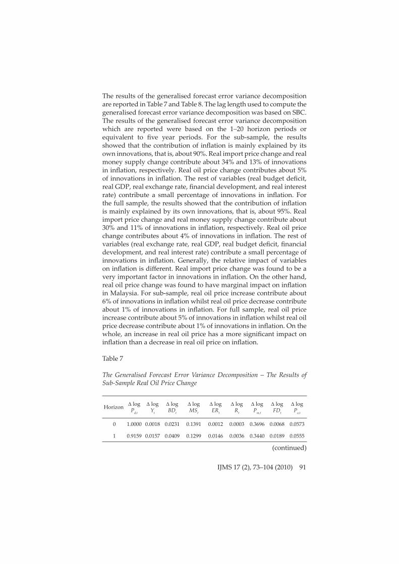
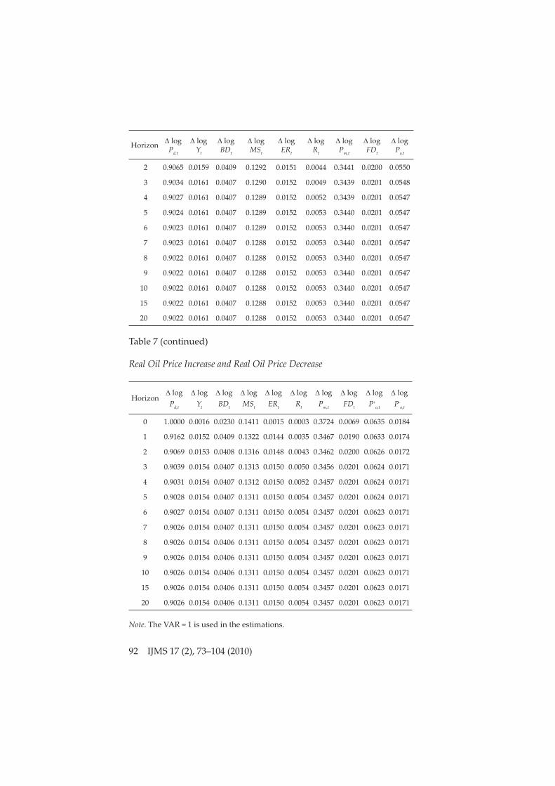
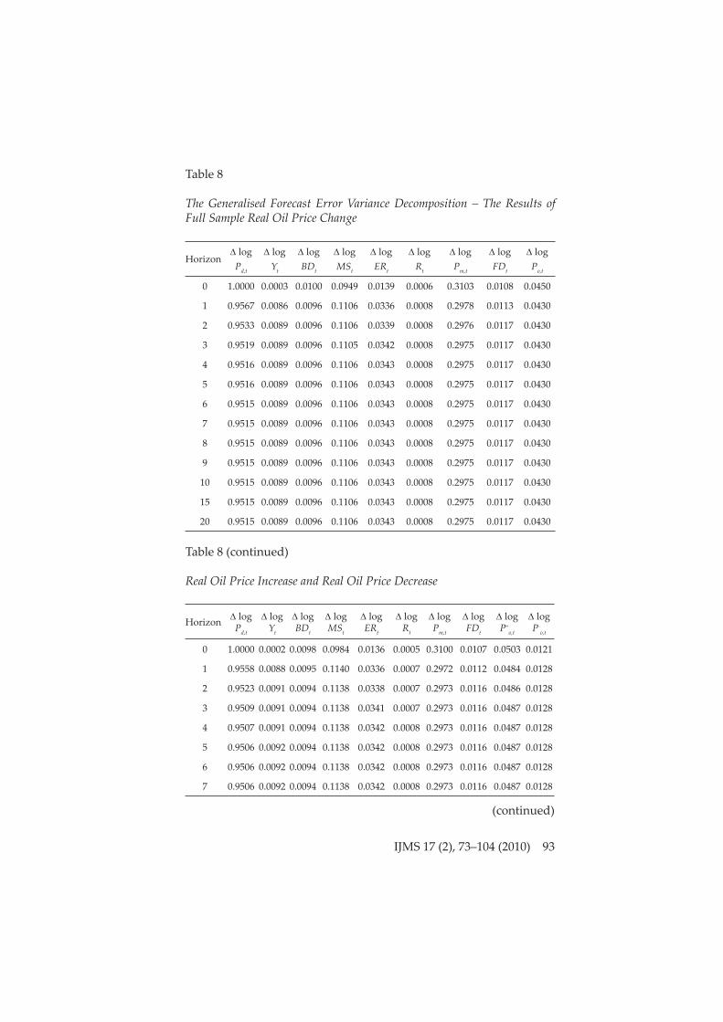
The results of the generalised forecast error variance decomposition are reported in Table 7 and Table 8. The lag length used to compute the generalised forecast error variance decomposition was based on SBC. The results of the generalised forecast error variance decomposition which are reported were based on the 1–20 horizon periods or equivalent to fi ve year periods. For the sub-sample, the results showed that the contribution of infl ation is mainly explained by its own innovations, that is, about 90%. Real import price change and real money supply change contribute about 34% and 13% of innovations in infl ation, respectively. Real oil price change contributes about 5% of innovations in infl ation. The rest of variables (real budget defi cit, real GDP, real exchange rate, fi nancial development, and real interest rate) contribute a small percentage of innovations in infl ation. For the full sample, the results showed that the contribution of infl ation is mainly explained by its own innovations, that is, about 95%. Real import price change and real money supply change contribute about 30% and 11% of innovations in infl ation, respectively. Real oil price change contributes about 4% of innovations in infl ation. The rest of variables (real exchange rate, real GDP, real budget defi cit, fi nancial development, and real interest rate) contribute a small percentage of innovations in infl ation. Generally, the relative impact of variables on infl ation is diff erent. Real import price change was found to be a very important factor in innovations in infl ation. On the other hand, real oil price change was found to have marginal impact on infl ation in Malaysia. For sub-sample, real oil price increase contribute about 6% of innovations in infl ation whilst real oil price decrease contribute about 1% of innovations in infl ation. For full sample, real oil price increase contribute about 5% of innovations in infl ation whilst real oil price decrease contribute about 1% of innovations in infl ation. On the whole, an increase in real oil price has a more signifi cant impact on infl ation than a decrease in real oil price on infl ation.
Table 7
The Generalised Forecast Error Variance Decomposition – The Results of Sub-Sample Real Oil Price Change
Horizon log Pd,t
log Yt
log BDt
log MSt
log ERt
log Rt
log Pm,t
log FDt
log Po,t
0 1.0000 0.0018 0.0231 0.1391 0.0012 0.0003 0.3696 0.0068 0.0573
1 0.9159 0.0157 0.0409 0.1299 0.0146 0.0036 0.3440 0.0189 0.0555
(continued)
http
://ijm
s.uu
m.e
du.m
y
92 IJMS 17 (2), 73–104 (2010)
Horizon log Pd,t
log Yt
log BDt
log MSt
log ERt
log Rt
log Pm,t
log FDt
log Po,t
2 0.9065 0.0159 0.0409 0.1292 0.0151 0.0044 0.3441 0.0200 0.0550
3 0.9034 0.0161 0.0407 0.1290 0.0152 0.0049 0.3439 0.0201 0.0548
4 0.9027 0.0161 0.0407 0.1289 0.0152 0.0052 0.3439 0.0201 0.0547
5 0.9024 0.0161 0.0407 0.1289 0.0152 0.0053 0.3440 0.0201 0.0547
6 0.9023 0.0161 0.0407 0.1289 0.0152 0.0053 0.3440 0.0201 0.0547
7 0.9023 0.0161 0.0407 0.1288 0.0152 0.0053 0.3440 0.0201 0.0547
8 0.9022 0.0161 0.0407 0.1288 0.0152 0.0053 0.3440 0.0201 0.0547
9 0.9022 0.0161 0.0407 0.1288 0.0152 0.0053 0.3440 0.0201 0.0547
10 0.9022 0.0161 0.0407 0.1288 0.0152 0.0053 0.3440 0.0201 0.0547
15 0.9022 0.0161 0.0407 0.1288 0.0152 0.0053 0.3440 0.0201 0.0547
20 0.9022 0.0161 0.0407 0.1288 0.0152 0.0053 0.3440 0.0201 0.0547
Table 7 (continued)
Real Oil Price Increase and Real Oil Price Decrease
Horizon log
Pd,t
log Yt
log BDt
log MSt
log ERt
log Rt
log Pm,t
log FDt
log P+
o,t
log P-
o,t
0 1.0000 0.0016 0.0230 0.1411 0.0015 0.0003 0.3724 0.0069 0.0635 0.0184
1 0.9162 0.0152 0.0409 0.1322 0.0144 0.0035 0.3467 0.0190 0.0633 0.0174
2 0.9069 0.0153 0.0408 0.1316 0.0148 0.0043 0.3462 0.0200 0.0626 0.0172
3 0.9039 0.0154 0.0407 0.1313 0.0150 0.0050 0.3456 0.0201 0.0624 0.0171
4 0.9031 0.0154 0.0407 0.1312 0.0150 0.0052 0.3457 0.0201 0.0624 0.0171
5 0.9028 0.0154 0.0407 0.1311 0.0150 0.0054 0.3457 0.0201 0.0624 0.0171
6 0.9027 0.0154 0.0407 0.1311 0.0150 0.0054 0.3457 0.0201 0.0623 0.0171
7 0.9026 0.0154 0.0407 0.1311 0.0150 0.0054 0.3457 0.0201 0.0623 0.0171
8 0.9026 0.0154 0.0406 0.1311 0.0150 0.0054 0.3457 0.0201 0.0623 0.0171
9 0.9026 0.0154 0.0406 0.1311 0.0150 0.0054 0.3457 0.0201 0.0623 0.0171
10 0.9026 0.0154 0.0406 0.1311 0.0150 0.0054 0.3457 0.0201 0.0623 0.0171
15 0.9026 0.0154 0.0406 0.1311 0.0150 0.0054 0.3457 0.0201 0.0623 0.0171
20 0.9026 0.0154 0.0406 0.1311 0.0150 0.0054 0.3457 0.0201 0.0623 0.0171
Note. The VAR = 1 is used in the estimations.
http
://ijm
s.uu
m.e
du.m
y
IJMS 17 (2), 73–104 (2010) 93
(continued)
Table 8
The Generalised Forecast Error Variance Decomposition – The Results of Full Sample Real Oil Price Change
Horizon log
Pd,t
log Yt
log BDt
log MSt
log ERt
log Rt
log Pm,t
log FDt
log Po,t
0 1.0000 0.0003 0.0100 0.0949 0.0139 0.0006 0.3103 0.0108 0.0450
1 0.9567 0.0086 0.0096 0.1106 0.0336 0.0008 0.2978 0.0113 0.0430
2 0.9533 0.0089 0.0096 0.1106 0.0339 0.0008 0.2976 0.0117 0.0430
3 0.9519 0.0089 0.0096 0.1105 0.0342 0.0008 0.2975 0.0117 0.0430
4 0.9516 0.0089 0.0096 0.1106 0.0343 0.0008 0.2975 0.0117 0.0430
5 0.9516 0.0089 0.0096 0.1106 0.0343 0.0008 0.2975 0.0117 0.0430
6 0.9515 0.0089 0.0096 0.1106 0.0343 0.0008 0.2975 0.0117 0.0430
7 0.9515 0.0089 0.0096 0.1106 0.0343 0.0008 0.2975 0.0117 0.0430
8 0.9515 0.0089 0.0096 0.1106 0.0343 0.0008 0.2975 0.0117 0.0430
9 0.9515 0.0089 0.0096 0.1106 0.0343 0.0008 0.2975 0.0117 0.0430
10 0.9515 0.0089 0.0096 0.1106 0.0343 0.0008 0.2975 0.0117 0.0430
15 0.9515 0.0089 0.0096 0.1106 0.0343 0.0008 0.2975 0.0117 0.0430
20 0.9515 0.0089 0.0096 0.1106 0.0343 0.0008 0.2975 0.0117 0.0430
Table 8 (continued)
Real Oil Price Increase and Real Oil Price Decrease
Horizon log Pd,t
log Yt
log BDt
log MSt
log ERt
log Rt
log Pm,t
log FDt
log P+
o,t
log P-
o,t
0 1.0000 0.0002 0.0098 0.0984 0.0136 0.0005 0.3100 0.0107 0.0503 0.0121
1 0.9558 0.0088 0.0095 0.1140 0.0336 0.0007 0.2972 0.0112 0.0484 0.0128
2 0.9523 0.0091 0.0094 0.1138 0.0338 0.0007 0.2973 0.0116 0.0486 0.0128
3 0.9509 0.0091 0.0094 0.1138 0.0341 0.0007 0.2973 0.0116 0.0487 0.0128
4 0.9507 0.0091 0.0094 0.1138 0.0342 0.0008 0.2973 0.0116 0.0487 0.0128
5 0.9506 0.0092 0.0094 0.1138 0.0342 0.0008 0.2973 0.0116 0.0487 0.0128
6 0.9506 0.0092 0.0094 0.1138 0.0342 0.0008 0.2973 0.0116 0.0487 0.0128
7 0.9506 0.0092 0.0094 0.1138 0.0342 0.0008 0.2973 0.0116 0.0487 0.0128
http
://ijm
s.uu
m.e
du.m
y
94 IJMS 17 (2), 73–104 (2010)
Horizon log Pd,t
log Yt
log BDt
log MSt
log ERt
logRt
log Pm,t
log FDt
log P+
o,t
log P-
o,t
8 0.9506 0.0092 0.0094 0.1138 0.0342 0.0008 0.2973 0.0116 0.0487 0.0128
9 0.9506 0.0092 0.0094 0.1138 0.0342 0.0008 0.2973 0.0116 0.0487 0.0128
10 0.9506 0.0092 0.0094 0.1138 0.0342 0.0008 0.2973 0.0116 0.0487 0.0128
15 0.9506 0.0092 0.0094 0.1138 0.0342 0.0008 0.2973 0.0116 0.0487 0.0128
20 0.9506 0.0092 0.0094 0.1138 0.0342 0.0008 0.2973 0.0116 0.0487 0.0128
Note: The VAR = 1 is used in the estimations.
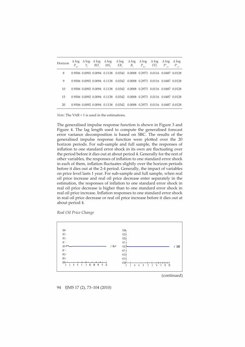
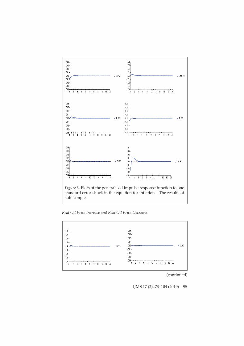
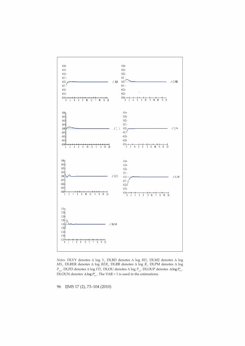
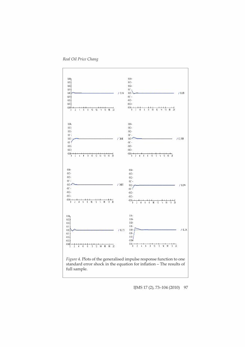
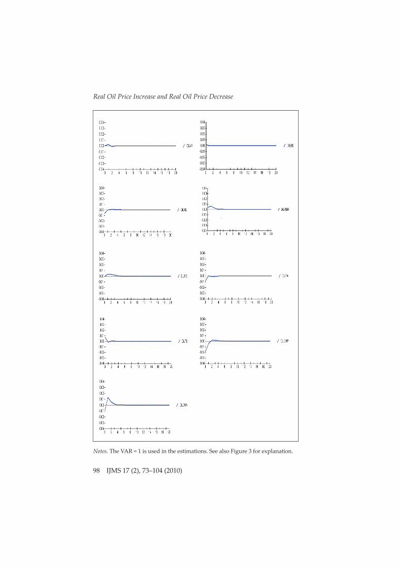
The generalised impulse response function is shown in Figure 3 and Figure 4. The lag length used to compute the generalised forecast error variance decomposition is based on SBC. The results of the generalised impulse response function were plott ed over the 20 horizon periods. For sub-sample and full sample, the responses of infl ation to one standard error shock in its own are fl uctuating over the period before it dies out at about period 4. Generally for the rest of other variables, the responses of infl ation to one standard error shock in each of them, infl ation fl uctuates slightly over the horizon periods before it dies out at the 2-4 period. Generally, the impact of variables on price level lasts 1 year. For sub-sample and full sample, when real oil price increase and real oil price decrease enter separately in the estimation, the responses of infl ation to one standard error shock in real oil price decrease is higher than to one standard error shock in real oil price increase. Infl ation responses to one standard error shock in real oil price decrease or real oil price increase before it dies out at about period 4.
Real Oil Price Change
(continued)
http
://ijm
s.uu
m.e
du.m
y
IJMS 17 (2), 73–104 (2010) 95
Figure 3. Plots of the generalised impulse response function to one standard error shock in the equation for infl ation – The results of sub-sample.
Real Oil Price Increase and Real Oil Price Decrease
(continued)
http
://ijm
s.uu
m.e
du.m
y
96 IJMS 17 (2), 73–104 (2010)
Notes. DLVY denotes log Yt. DLBD denotes log BDt. DLM2 denotes log MSt. DLRER denotes log RERt. DLRB denotes log Rt. DLPM denotes log Pm,t. DLFD denotes log FDt. DLOU denotes log Po,t. DLOUP denotes toP ,log . DLOUN denotes toP ,log . The VAR = 1 is used in the estimations.
http
://ijm
s.uu
m.e
du.m
y
IJMS 17 (2), 73–104 (2010) 97
Real Oil Price Chang
Figure 4. Plots of the generalised impulse response function to one standard error shock in the equation for infl ation – The results of full sample.
http
://ijm
s.uu
m.e
du.m
y
98 IJMS 17 (2), 73–104 (2010)
Real Oil Price Increase and Real Oil Price Decrease
Notes. The VAR = 1 is used in the estimations. See also Figure 3 for explanation.
http
://ijm
s.uu
m.e
du.m
y
IJMS 17 (2), 73–104 (2010) 99
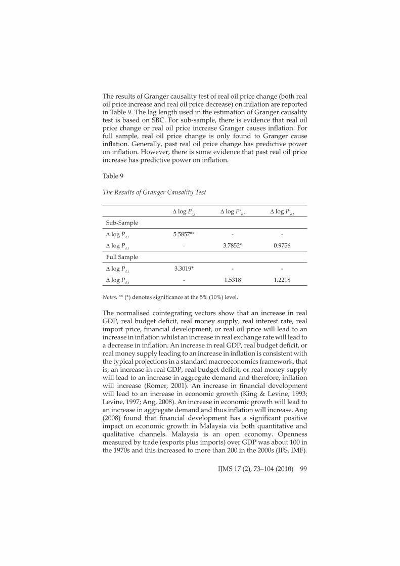
The results of Granger causality test of real oil price change (both real oil price increase and real oil price decrease) on infl ation are reported in Table 9. The lag length used in the estimation of Granger causality test is based on SBC. For sub-sample, there is evidence that real oil price change or real oil price increase Granger causes infl ation. For full sample, real oil price change is only found to Granger cause infl ation. Generally, past real oil price change has predictive power on infl ation. However, there is some evidence that past real oil price increase has predictive power on infl ation.
Table 9
The Results of Granger Causality Test
log Po,t log P+o,t log P-
o,t
Sub-Sample
log Pd,t 5.5857** - -
log Pd,t - 3.7852* 0.9756
Full Sample
log Pd,t 3.3019* - -
log Pd,t - 1.5318 1.2218
Notes. ** (*) denotes signifi cance at the 5% (10%) level.
The normalised cointegrating vectors show that an increase in real GDP, real budget defi cit, real money supply, real interest rate, real import price, fi nancial development, or real oil price will lead to an increase in infl ation whilst an increase in real exchange rate will lead to a decrease in infl ation. An increase in real GDP, real budget defi cit, or real money supply leading to an increase in infl ation is consistent with the typical projections in a standard macroeconomics framework, that is, an increase in real GDP, real budget defi cit, or real money supply will lead to an increase in aggregate demand and therefore, infl ation will increase (Romer, 2001). An increase in fi nancial development will lead to an increase in economic growth (King & Levine, 1993; Levine, 1997; Ang, 2008). An increase in economic growth will lead to an increase in aggregate demand and thus infl ation will increase. Ang (2008) found that fi nancial development has a signifi cant positive impact on economic growth in Malaysia via both quantitative and qualitative channels. Malaysia is an open economy. Openness measured by trade (exports plus imports) over GDP was about 100 in the 1970s and this increased to more than 200 in the 2000s (IFS, IMF).
http
://ijm
s.uu
m.e
du.m
y
100 IJMS 17 (2), 73–104 (2010)
A more open economy increases economy inter-dependence through international trade and fi nance. Thus an increase in real import price or real oil price will have a more signifi cant impact on infl ation in Malaysia as it becomes more open to the world. Cologni and Manera (2008) also reported that an increase in oil price has a signifi cant impact on infl ation in most G-7 countries. O’Neill, Penm, and Terrell (2008) found that an increase in oil price will lead an increase in expectation of higher infl ation in major O rganisation for Economic Co-operation and Development (OECD) countries.
In this study, an increase in real oil price was found to have a more signifi cant impact on infl ation than a decrease in real oil price. Cunado and De Gracia (2005) also found that the relationship between real oil price change and infl ation is asymmetric in Malaysia. Moreover, the study reported that there is some evidence of Granger causality from real oil price change, which is measured in domestic currency to infl ation. This study also found that past real oil price change has predictive power on infl ation. Moreover, there is some evidence that past real oil price increase has predictive power on infl ation. An increase in real exchange rate is found to decrease infl ation. Mansor (2003) also reported the importance of exchange rate in stability for the Malaysian economy. Appreciation in real exchange rate will help to reduce infl ation pressure through cheaper imports of goods and services (MOF, 2006, p. 2).
The main determinants of infl ation in Malaysia are real GDP, real import price, and real money supply. Real oil price and other variables examined are relatively less important in the determination of infl ation. One reason of less importance of real oil price on infl ation is that oil price in Malaysia is subsidised and controlled, and thus its impact on infl ation is less signifi cant. Nonetheless, real oil price change has predictive power on infl ation. An increase in oil price in the world will likely increase infl ation in Malaysia. Malaysia is a small open economy. External shock such as changes in import price has a stronger impact on infl ation in Malaysia. Thus an increase in infl ation in the world will lead to an increase in infl ation in Malaysia.
The policy implications of the study are a set of variables should be checked in order to control infl ation. Fiscal and monetary policies can be used for this purpose. During the Asian fi nancial crisis, 19971998, the government implemented a budget defi cit and strengthened its fi nancial system to promote economic growth. A package of government expenditure and expansionary monetary policy such as low interest rate, were used to stimulate economic growth during the
http
://ijm
s.uu
m.e
du.m
y
IJMS 17 (2), 73–104 (2010) 101
economic downturn in the early of 2000s. A high economic growth will enhance aggregate demand in the economy and thus infl ation will increase. A sound fi nancial system is important to promote economic growth. A higher economic growth will lead to a higher infl ation. Thus it is important for the government to develop its fi nancial system according to the state of the economy.
Malaysia is a small open economy. The impact of infl ation from abroad can be easily transmitt ed to the economy. A strong exchange rate could help reduce the impact of imported infl ation. A fi xed exchange rate ringgit against the American dollar was implemented during the Asian fi nancial crisis. For the period from 2 September 1998 to 31 December 2003, the exchange rate was fi xed at RM3.80 to one US dollar (Bank Negara Malaysia, 1999, p. 584). It has been argued that generally the fi xed exchange rate has provided a strong foundation to improve international reserve and trade balance. An increase in the world oil price will defi nitely aff ect infl ation in Malaysia. To reduce the impact of high oil price in the world in the 2000s, the government has implemented a package of economic relief such as road tax reduction, fuel subsidy, and price control. In a longer period, alternate use of fuel may introduced and also the society would be educated to use energy effi ciently.
Concluding Remarks
This study has investigated the determination of infl ation in Malaysia. For the sub-sample, the results of cointegration tests showed that there is one cointegrating vector. Conversely for the full sample, the results of cointegration tests showed that there is at least one cointegrating vector. The results of the likelihood ratio test statistics showed that there are many factors that are important in infl uencing infl ation in Malaysia. The results of the normalised cointegrating vectors showed that an increase in real GDP, real budget defi cit, real money supply, real interest rate, real import price, fi nancial development, or real oil price will lead to an increase in infl ation whilst an increase in real exchange rate will lead to a decrease in infl ation.
The results of the generalised forecast error variance decomposition showed that the relative impact of variables on infl ation is diff erent. Real import price change was found to be one of the most important factors in innovations in infl ation. On the other hand, real oil price change was found to have marginal impact on infl ation in Malaysia. Moreover, an increase in real oil price was found to have a more signifi cant impact on infl ation than a decrease in real oil price. Thus
http
://ijm
s.uu
m.e
du.m
y
102 IJMS 17 (2), 73–104 (2010)
there is asymmetric relationship between real oil price change and infl ation in Malaysia. The results of the generalised impulse response function showed that the impact of variables examined on infl ation lasts about one year. There is evidence that real oil price change Granger causes infl ation.
The main determinants of infl ation in Malaysia are real GDP, real import price, and real money supply. Real oil price and other variables examined are relatively less important in the determination of infl ation. An increase in real oil price has a more signifi cant impact on infl ation than a decrease in real oil price on infl ation. Moreover, real oil price change has predictive power on infl ation. Malaysia is a small open economy and thus it is vulnerable to external shock such as changes in import price. An increase in infl ation in the world will lead to an increase in infl ation in Malaysia. On the whole, there are a few important factors that cause infl ation in Malaysia, thus managing infl ation requires special att ention for these factors.
Acknowledgement
The author would like to thank the reviewer of the journal for the comments on an earlier version of this paper. All remaining errors are the author’s.
References
Ang, J. B. (2008). What are the mechanism linking fi nancial development and economic growth in Malaysia? Economic Modelling, 25(1), 38–53.
Bahmani-Oskooee, M., & Rehman, H. (2005). Stability of the money demand function in Asian developing countries. Applied Economics, 37, 773–792.
Baltagi, B. H., Demetriades, P.O., & Law, S. H. (2009). Financial development and openness: Evidence from panel data. Journal of Development Economics, 89(2), 285–296.
Bank Negara Malaysia (1999). The central bank and the fi nancial system in Malaysia: A decade of change 1989–1999. Kuala Lumpur: Bank Negara Malaysia.
Chang Y., & Wong, J. F. (2003). Oil price fl uctuations and Singapore economy. Energy Policy, 31, 1151–1165.
Cheng, M. Y., & Tan, H. B. (2002). Infl ation in Malaysia. International Journal of Social Economics, 29(5), 411–425.
http
://ijm
s.uu
m.e
du.m
y
IJMS 17 (2), 73–104 (2010) 103
Cologni, A., & Manera, M. (2008). Oil prices, infl ation and interest rates in a structural cointegrated VAR model for the G-7 countries. Energy Economics, 30(3), 856–888.
Cunado, J., & De Gracia, F. P. (2005). Oil prices, economic activity and infl ation: Evidence for some Asian countries. The Quarterly Review of Economics and Finance, 45, 65–83.
Daniels, J. P., & VanHoose, D. D. (2005). International monetary and fi nancial economics (3rd ed.). Mason, Ohio: Thomson: South-Western.
Dickey, D. A., & Fuller, W. A. (1979). Distribution of the estimators for autoregressive time series with a unit root. Journal of the American Statistical Association, 74(366), 427–431.
Elliott , G., Rothenberg, T. J., & Stock, J. H. (1996). Effi cient tests for an autoregressive unit root. Econometrica, 64, 813–836.
Engle, R. F., & Granger, C. W. J. (1987). Co-integration and error correction: Representation, estimation, and testing. Econometrica, 55(2), 251–276.
Granger, C. W. J. (1969). Investigating causal relations by econometric models and cross spectral models. Econometrica, 37, 424–438.
Johansen, S. (1988). Statistical analysis of cointegration vectors. Journal of Economic Dynamics and Control, 12(2–3), 231–254.
King, R., & Levine, R. (1993). Finance and growth: Schumpeter might be right. The Quarterly Journal of Economics, 108(3), 717–737.
Koop, G., Pesaran, M. H., & Pott er, S. M. (1996). Impulse response analysis in nonlinear multivariate models. Journal of Econometrics, 74, 119–147.
Kwiatkowski, D., Phillips, P. C. B., Schmidt, P., & Shin, Y. (1992). Testing the null hypothesis of stationary against the alternative of a unit root. Journal of Econometrics, 54, 159–178.
Levine, R. (1997). Financial development and economic growth: Views and agenda. Journal of Economic Literature, 35(2), 688–726.
Linnemann, L. (2005). Can raising interest rates increase infl ation? Economics lett ers, 87, 307–311.
MacKinnon, J. G. (1996). Numerical distribution functions for unit root and cointegration tests. Journal of Applied Econometrics, 11(6), 601–618.
Mansor, H. I. (2003). International disturbances and domestic macroeconomic fl uctuations in Malaysia. ASEAN Economic Bulletin, 20(1), 11–30.
Ministry of Finance Malaysia (MOF) (1999). Economic report 1999/2000. Kuala Lumpur: Print Nasional Malaysia Berhad.
Ministry of Finance Malaysia (MOF) (2006). Economic report 2006/2007. Kuala Lumpur: Print Nasional Malaysia Berhad.
http
://ijm
s.uu
m.e
du.m
y
104 IJMS 17 (2), 73–104 (2010)
Mork, K. (1989). Oil and the macroeconomy when prices go up and down: An extension of Hamilton’s results. Journal of Political Economy, 97, 740–744.
Ng, S., & Perron, P. (2001). Lag length selection and the construction of unit root tests with good size and power. Econometrica, 69(6), 1519–1554.
O’Neill, T. J., Penm, J., & Terrell, R. D. (2008). The role of higher oil prices: A case of major developed countries. Research in Finance, 24, 287–299.
Pesaran, H., & Shin, Y. (1998). Generalized impulse response analysis in linear multivariate models. Economics Lett ers, 58, 17–29.
Phillips, P. C. B., & Perron, P. (1988). Testing for a unit root in time series regression. Biometrika, 75(2), 335–346.
Rajan, R. G., & Zingales, L. (2003). The great reversals: The politics of fi nancial development in the 20th century. Journal of Financial Economics, 69, 5–50.
Romer, D. (2001). Advanced macroeconomics (2nd ed.). Singapore: McGraw-Hill.
Sims, C. (1980). Macroeconomics and reality. Econometrica, 48, 1–48.
http
://ijm
s.uu
m.e
du.m
y