Embed Size (px)
Citation preview

Infinitesimal Methods inMathematical Economics
Robert M. Anderson1
Department of Economics
and Department of Mathematics
University of California at BerkeleyBerkeley, CA 94720, U.S.A.
and
Department of Economics
Johns Hopkins UniversityBaltimore, MD 21218, U.S.A.
January 20, 2008
1The author is grateful to Marc Bettzuge, Don Brown, Hung-Wen Chang, Gerard Debreu, Eddie Dekel-Tabak, Greg Engl,Dmitri Ivanov, Jerry Keisler, Peter Loeb, Paul MacMillan, MikeMagill, Andreu Mas-Colell, Max Stinchcombe, Cathy Wein-berger and Bill Zame for their helpful comments. Financial sup-port from Deutsche Forschungsgemeinschaft, Gottfried-Wilhelm-Leibniz-Forderpreis is gratefully acknowledged.

Contents
0 Preface v
1 Nonstandard Analysis Lite 11.1 When is Nonstandard Analysis Useful? . . . . 1
1.1.1 Large Economies . . . . . . . . . . . . 21.1.2 Continuum of Random Variables . . . 41.1.3 Searching For Elementary Proofs . . . 4
1.2 Ideal Elements . . . . . . . . . . . . . . . . . 51.3 Ultraproducts . . . . . . . . . . . . . . . . . . 61.4 Internal and External Sets . . . . . . . . . . . 91.5 Notational Conventions . . . . . . . . . . . . . 111.6 Standard Models . . . . . . . . . . . . . . . . 121.7 Superstructure Embeddings . . . . . . . . . . 141.8 A Formal Language . . . . . . . . . . . . . . . 161.9 Transfer Principle . . . . . . . . . . . . . . . . 161.10 Saturation . . . . . . . . . . . . . . . . . . . . 181.11 Internal Definition Principle . . . . . . . . . . 191.12 Nonstandard Extensions, or Enough Already
with the Ultraproducts . . . . . . . . . . . . . 201.13 Hyperfinite Sets . . . . . . . . . . . . . . . . . 211.14 Nonstandard Theorems Have Standard Proofs 22
2 Nonstandard Analysis Regular 232.1 Warning: Do Not Read this Chapter . . . . . 23
i
ii CONTENTS
2.2 A Formal Language . . . . . . . . . . . . . . . 232.3 Extensions of L . . . . . . . . . . . . . . . . . 252.4 Assigning Truth Value to Formulas . . . . . . 282.5 Interpreting Formulas in Superstructure Em-
beddings . . . . . . . . . . . . . . . . . . . . . 322.6 Transfer Principle . . . . . . . . . . . . . . . . 332.7 Internal Definition Principle . . . . . . . . . . 342.8 Nonstandard Extensions . . . . . . . . . . . . 352.9 The External Language . . . . . . . . . . . . . 362.10 The Conservation Principle . . . . . . . . . . 37
3 Real Analysis 393.1 Monads . . . . . . . . . . . . . . . . . . . . . 393.2 Open and Closed Sets . . . . . . . . . . . . . 443.3 Compactness . . . . . . . . . . . . . . . . . . 453.4 Products . . . . . . . . . . . . . . . . . . . . . 483.5 Continuity . . . . . . . . . . . . . . . . . . . . 493.6 Differentiation . . . . . . . . . . . . . . . . . . 523.7 Riemann Integration . . . . . . . . . . . . . . 533.8 Differential Equations . . . . . . . . . . . . . . 54
4 Loeb Measure 574.1 Existence of Loeb Measure . . . . . . . . . . . 574.2 Lebesgue Measure . . . . . . . . . . . . . . . . 614.3 Representation of Radon Measures . . . . . . 624.4 Lifting Theorems . . . . . . . . . . . . . . . . 634.5 Weak Convergence . . . . . . . . . . . . . . . 65
5 Large Economies 695.1 Preferences . . . . . . . . . . . . . . . . . . . 705.2 Hyperfinite Economies . . . . . . . . . . . . . 745.3 Loeb Measure Economies . . . . . . . . . . . . 745.4 Budget, Support and Demand Gaps . . . . . . 755.5 Core . . . . . . . . . . . . . . . . . . . . . . . 76
CONTENTS iii
5.6 Approximate Equilibria . . . . . . . . . . . . . 985.7 Pareto Optima . . . . . . . . . . . . . . . . . 985.8 Bargaining Set . . . . . . . . . . . . . . . . . 985.9 Value . . . . . . . . . . . . . . . . . . . . . . . 995.10 “Strong” Core Theorems . . . . . . . . . . . . 99
6 Continuum of Random Variables 1016.1 The Problem . . . . . . . . . . . . . . . . . . 1016.2 Loeb Space Construction . . . . . . . . . . . . 1036.3 Price Adjustment Model . . . . . . . . . . . . 105
7 Noncooperative Game Theory 111
8 Stochastic Processes 113
9 Translation 115
10 Further Reading 119
A Existence Proof 121

iv CONTENTS
Chapter 0
Preface
Nonstandard analysis is a mathematical technique widelyused in diverse areas in pure and applied mathematics, in-cluding probability theory, mathematical physics, functionalanalysis. Our primary goal is to provide a careful devel-opment of nonstandard methodology in sufficient detail toallow the reader to use it in diverse areas in mathematicaleconomics. This requires some work in mathematical logic.More importantly, it requires a careful study of the nonstan-dard treatment of real analysis, measure theory, topologicalspaces, and so on.
Chapter 1 provides an informal description of nonstan-dard methods which should permit the reader to understandthe mathematical Chapters 3, 4 and 9, as well as Chapters 5,6, 7 and 8 which provide applications in Economics. Chapter2 provides a precise statement of the fundamental results onnonstandard models, using tools from mathematical logic.Most readers will find it better to browse through the proofsin Chapter 3 before tackling Chapter 2; many readers willchoose to skip Chapter 2 entirely! The proof of the exis-tence of nonstandard models is trivial but tedious, and so isdeferred to Appendix A.
v
vi CHAPTER 0. PREFACE
This is an expanded version of Anderson (1992), a Chap-ter in Volume IV of the Handbook of Mathematical Eco-nomics. This first handout contains Chapters 1–3 and theBibliography. Chapters 4 and 5 and part of Chapter 6 aredone, apart from minor revisions to be made based on theexperience in the first few weeks of teaching; they will behanded out in a few weeks. The remainder of the the chap-ters listed in the contents are phantoms at this point; theywill be written and distributed over the course of the semester.

Chapter 1
Nonstandard AnalysisLite
1.1 When is Nonstandard Analysis
Useful?
Nonstandard analysis can be used to formalize most areas ofmodern mathematics, including real and complex analysis,measure theory, probability theory, functional analysis, andpoint set topology; algebra is less amenable to nonstandardtreatments, but even there significant applications have beenfound.
Complicated ε—δ arguments can usually be replaced bysimpler, more intuitive nonstandard arguments involving in-finitesimals. Given the dependence of work in mathemati-cal economics on arguments from real analysis at the levelof Rudin(1976) or Royden (1968), a very large number ofpapers could be significantly simplified using nonstandardarguments. Unfortunately, there is a significant barrier tothe widespread adoption of nonstandard arguments for thesekinds of problems, a barrier very much akin to the problems
1
2 CHAPTER 1. NONSTANDARD ANALYSIS LITE
associated with the adoption of a new technological stan-dard. Few economists are trained in nonstandard analysis,so papers using the methodology are necessarily restrictedto a small audience. Consequently, relatively few authorsuse the methodology if more familiar methods will suffice.Therefore, the incentives to learn the methodology are lim-ited. Accordingly, the use of nonstandard methods in eco-nomics has largely been limited to certain problems in whichthe advantages of the methodology are greatest.
1.1.1 Large Economies
Most of the work in Economics using nonstandard methodshas occurred in the literature on large economies. Supposeχn : An → P × Rk
+ is a sequence of exchange economieswith |An| → ∞. In other words, An is the set of agents and|An| the number of agents in the nth economy, P a set ofpreferences, and χn assigns to each agent a preference andan endowment vector. A natural approach to analyzing thesequence χn is to formulate a notion of a limit economy χ :A → P ×Rk
+. This limit economy can be formulated with Abeing either a nonatomic measure space or a hyperfinite set–anonstandard construction. The properties of measure spacesand hyperfinite sets are closely analogous. Indeed, using theLoeb measure construction which we describe in Chapter4, a hyperfinite set can be converted into a measure space.The theory of economies with a hyperfinite set of agents isanalogous in many respects to the theory of economies witha measure space of agents.
However, there are certain phenomena that can occur inhyperfinite economies which are ruled out by the measure-theoretic formulation. For the most part, these relate tosituations in which a small proportion of the agents are en-

1.1. WHEN IS NONSTANDARD ANALYSIS USEFUL? 3
dowed with, or consume, a substantial fraction of the goodspresent in the economy. In the hyperfinite context, certainconditions inherent in the measure-theoretic formulation canbe seen to be strong endogenous assumptions. Using hyper-finite exchange economies, we can state exogenous assump-tions which imply the endogenous assumptions inherent inthe measure-theoretic formulation, as well as explore the be-havior of economies in which the endogenous assumptionsfail.
The power of the nonstandard methodology is seen mostclearly at the next stage, in which one deduces theoremsabout the sequence χn from the theorems about the limitχ. A central result known as the Transfer Principle assertsthat any property which can be formalized in a particularformal language and which holds for χ must also hold for χn
for sufficiently large n. Viewed in this context, the TransferPrinciple functions as a sweeping generalization of the con-vergence theorems that can be formulated using topologyand measure theory. The Transfer Principle converts resultsabout the limit economy χ into limiting results about the se-quence χn in a few lines of argument. Consequently, for thoseproperties which hold both in measure-theoretic and hyperfi-nite economies, nonstandard analysis provides a very efficienttool to derive limit theorems for large finite economies. Onthe other hand, in the situations in which the behavior of themeasure-theoretic and hyperfinite economies differ, it is thehyperfinite economy rather than the measure-theoretic econ-omy which captures the behavior of large finite economies.The literature on large economies is discussed in Chapter 5.

4 CHAPTER 1. NONSTANDARD ANALYSIS LITE
1.1.2 Continuum of Random Variables
Probability theory is currently the most active field for ap-plications of nonstandard analysis. Since probabilistic con-structions are widely used in general equilibrium theory, gametheory and finance, these seem fruitful areas for further ap-plications of nonstandard methodology.
Nonstandard analysis provides an easy resolution of theso-called continuum of random variables problem. Given astandard measure space (A,A, μ) and an uncountable fam-ily of independent identically distributed random variablesXλ : A → R, one would like to assert that there is no aggre-gate uncertainty; in other words, the empirical distributionof the Xλ’s equals the theoretical distributuion with proba-bility one. Typically, however, the set of a ∈ A for whichthe empirical distribution of the Xλ’s equals the theoreticaldistribution is not measurable; by extending μ, it can beassigned any measure between 0 and 1. Note that, with alarge finite number of random variables, the measurabilityissue does not even arise. Thus, the problem is a pathologyarising from the formulation of measure theory, and not aproblem of large finite systems. If A is a hyperfinite set,and μ is the Loeb measure, then the empirical distributiondoes equal the theoretical distribution with probability one.Moreover, as in the large economies literature, the Trans-fer Principle can be used to deduce asymptotic properties oflarge finite systems. The Continuum of Random VariablesProblem is discussed in Chapter 6.
1.1.3 Searching For Elementary Proofs
Nonstandard analysis allows one to replace many measure-theoretic arguments by discrete combinatoric arguments. Forexample, the Shapley-Folkman Theorem plays the same role
1.2. IDEAL ELEMENTS 5
in hyperfinite sets as Lyapunov’s Theorem plays in nonatomicmeasure spaces. Thus, nonstandard analysis is an effectivetool for determining exactly which parts of a given proof re-ally depend on arguments in analysis, and which follow frommore elementary considerations. Occasionally, it is possibleto replace every step in a proof by an elementary argument;as a consequence, one obtains a proof using neither nonstan-dard analysis nor measure theory. Examples are discussedin Chapter 9.
1.2 Ideal Elements
Leibniz’ formulation of calculus was based on the notion of aninfinitesimal. Mathematics has frequently advanced throughthe introduction of ideal elements to provide solutions toequations. The Greeks were horrified to discover that theequation x2 = 2 has no rational solution; this problem wasresolved by the introduction of the ideal element
√2; ulti-
mately, the real numbers were defined as the completion ofthe rationals. Similarly, the complex numbers were createdby the introduction of the ideal element i =
√−1. Leibniz
introduced infinitesimals as ideal elements which, while notzero, were smaller than any positive real number. Thus, aninfinitesimal is an ideal element providing a solution to thefamily of equations
x > 0; x < 1, x <1
2, x <
1
3, . . . . (1.1)
Infinitesimals played a key role in Leibniz’ formulation of cal-culus. For example, the derivative of a function was definedas the slope of the function over an interval of infinitesimallength. Leibniz asserted that the real numbers, augmentedby the addition of infinitesimals, obeyed all the same rules
6 CHAPTER 1. NONSTANDARD ANALYSIS LITE
as the ordinary real numbers. Unfortunately, neither Leib-niz nor his successors were able to develop a formulationof infinitesimals which was free from contradictions. Con-sequently, in the middle of the nineteenth century, the ε–δformulation replaced infinitesimals as the generally acceptedfoundation of calculus and real analysis.
In 1961, Abraham Robinson discovered that model the-ory, a branch of mathematical logic, provided a satisfactoryfoundation for the use of infinitesimals in analysis. In theremainder of Section 1, we will provide an informal descrip-tion of a model of the nonstandard real numbers. In Section2, we will provide a formal description of nonstandard mod-els, along with a precise statement of the rules of inferencewhich are allowed in reasoning about nonstandard models.The proof of the underlying theorems which justify the rulesof inference will be presented in the Appendix.
1.3 Ultraproducts
A very simple construction which produces elements with in-finitesimal properties is RN, the space of real sequences. Wecan embed R into RN by mapping each r ∈ R to the con-stant sequence r = (r, r, r, . . .). Now consider the sequencedefined by xn = 1
n. Let R++ denote the set of strictly posi-
tive real numbers. Given any r ∈ R++, observe that xn < rn
for all but a finite number of values of n. In other words, ifwe were to define a relation <F on RN by
x <F y ⇐⇒ xn < yn for all but a finite number of n ∈ N,(1.2)
then x would be infinitesimal in the sense that x <F r forevery positive r ∈ R. Unfortunately, this very simple con-struction does not yield a satisfactory theory of infinitesi-

1.3. ULTRAPRODUCTS 7
mals. For example, consider y defined by yn = 2 for n oddand yn = 0 for n even. Neither y <F 1 nor 1 <F y is true;in other words, <F is only a partial order on RN. In or-der to construct a satisfactory theory of infinitesimals, weconsider a slightly more elaborate construction, known as anultraproduct.
Definition 1.3.1 A free ultrafilter on N is a collection U ofsubsets of N satisfying the following properties:
1. if A, B ∈ U , then A ∩ B ∈ U ;
2. if A ∈ U and A ⊂ B ⊂ N, then B ∈ U ;
3. if A is finite, then A ∈ U ;
4. if A ⊂ N, either A ∈ U or N \ A ∈ U .
Remark 1.3.2 Note that by item 4 of Definition 1.3.1, wemust have either {2, 4, 6, . . .} ∈ U or {1, 3, 5, . . .} ∈ U , butnot both by items 1 and 3.
Proposition 1.3.3 Suppose N = A1 ∪ . . .∪An with n ∈ N,and Ai ∩ Aj = ∅ for i = j. Then Ai ∈ U for exactly one i.
Proof: Let Bi = N \ Ai. If there is no i such that Ai ∈ U ,then Bi ∈ U for each i. Then ∅ = B1 ∩ (B2 ∩ . . . ∩ (Bn−1 ∩Bn) . . .) ∈ U by n−1 applications of Property 1 of Definition1.3.1, which contradicts Property 3 (since ∅ is finite). Thus,Ai ∈ U for some i. If Ai ∈ U and Aj ∈ U with i = j, then∅ = Ai ∩ Aj ∈ U , again contradicting Property 3. Thus,Ai ∈ U for exactly one i.
Definition 1.3.4 The equivalence relation =U on RN is de-fined by
x =U y ⇐⇒ {n : xn = yn} ∈ U . (1.3)
8 CHAPTER 1. NONSTANDARD ANALYSIS LITE
Given x ∈ RN, let [x] denote the equivalence class of xwith respect to the equivalence relation =U . The set of non-standard real numbers, denoted *R and read “star R”, is{[x] : x ∈ RN}.
Any relation on R can be extended to *R. In particular,given [x], [y] ∈ *R, we can define
[x] <U [y] ⇐⇒ {n : xn < yn} ∈ U . (1.4)
The reader will easily verify that this definition is indepen-dent of the particular representatives x and y chosen fromthe equivalence classes [x], [y].
Proposition 1.3.5 Suppose [x], [y] ∈ *R. Then exactly oneof [x] <U [y], [x] =U [y], or [x] >U [y] is true.
Proof: Let A = {n ∈ N : xn < yn}, B = {n ∈ N : xn =yn}, and C = {n ∈ N : xn > yn}. By Proposition 1.3.3,exactly one of A, B or C is in U .
Example 1.3.6 Let x ∈ RN be defined by xn = 1n, and r =
(r, r, . . .) for r ∈ R. If r > 0, then {n : xn < rn} ∈ U , sinceits complement is finite. Thus, [x] <U [r] for all r ∈ R++, i.e.[x] is an infinitesimal. We write [x] [y] if [x]− [y] (definedto be [z] where zn = xn − yn) is an infinitesimal.
Definition 1.3.7 [x] ∈ *R is said to be infinite if [x] >U mfor all m ∈ N.
Given any function f : R → R, we can define a function*f : *R → R by
*f([x]) = [(f(x1), f(x2), ...)]. (1.5)
In other words, *f is defined by evaluating f pointwise onthe components of x.
1.4. INTERNAL AND EXTERNAL SETS 9
1.4 Internal and External Sets
In order to work with the nonstandard real numbers, weneed to be able to talk about subsets of *R. We extend theultraproduct construction to sets by considering sequences in(P(R))N, where P(R) is the collection of all subsets of R,and extending the equivalence relation =U from Definition1.3.4.
Definition 1.4.1 Suppose A, B ∈ (P(R))N, [x] ∈ *R. Wedefine an equivalence relation =U by
A =U B ⇐⇒ {n : An = Bn} ∈ U . (1.6)
Let [A] denote the equivalence class of A. We define
[x] ∈U [A] ⇐⇒ {n : xn ∈ An} ∈ U .1 (1.7)
Note that [A] is not a subset of *R; it is an equivalence classof sequences of sets of real numbers, not a set of equiva-lence classes of sequences of real numbers. However, we canassociate it with a subset of *R in a natural way, as follows.
Definition 1.4.2 (Mostowski Collapsing Function)Given A ∈ (P(R))N, define a set M([A]) ⊂ *R by
M([A]) = {[x] ∈ *R : [x] ∈U [A]}. (1.8)
A set B ⊂ *R is said to be internal if B = M([A]) for someA ∈ (P(R))N; otherwise, it is said to be external. A functionis internal if its graph is internal.
1As above, the reader will have no trouble verifying that the defini-tion does not depend on the choice of representatives from the equiva-lence classes.

10 CHAPTER 1. NONSTANDARD ANALYSIS LITE
Definition 1.4.3 Suppose B ⊂ R. Define *B = M([A]),where A ∈ (P(R))N is the constant sequence An = B for alln ∈ N.
Example 1.4.4 The set of nonstandard natural numbers is
*N = {[x] ∈ *R : {n : xn ∈ N} ∈ U}. (1.9)
Let N = {[n] : n ∈ N}. Then N ⊂ *N. Indeed, N is aproper subset of *N, as can be seen by considering [x], wherexn = n for all n ∈ N. If m ∈ N, {n : xn = mn} = {m} ∈ U ,so [x] = [m].
Proposition 1.4.5 *N \ N is external.
Proof: Suppose *N \ N = M([A]). We shall derive a con-tradiction by constructing [y] ∈ *N \ N with [y] ∈ M([A]).
Let J = {n : An ⊂ N}. We may choose x ∈ RN suchthat xn ∈ An \ N for n ∈ N \ J , and xn = 0 for n ∈ J .Therefore, {n ∈ N : xn ∈ N} = ∅, so [x] ∈ *N. SinceM([A]) ⊂ *N, [x] ∈ M([A]), so N \ J ∈ U , so J ∈ U .Without loss of generality, we may assume that An ⊂ N forall n ∈ N.
For m ∈ N, let Tm = {n ∈ N : m ∈ An}; since [m] ∈M([A]), Tm ∈ U . For m ∈ N ∪ {0}, let
Sm = {n ∈ N : An ⊂ {m, m + 1, m + 2, . . .}}. (1.10)
Then Sm = ∩m−1k=1 Tk, so Sm ∈ U . S0 = N. Let S∞ =
∩m∈NSm = {n ∈ N : An = ∅}. If S∞ ∈ U , then M([A]) = ∅,a contradiction since *N \ N = ∅ by Example 1.4.4. Hence,S∞ ∈ U .
Define a sequence y ∈ RN by yn = m if n ∈ Sm+1 \Sm+2,yn = 0 for n ∈ S∞. Then {n : yn ∈ N} = N \ S∞ ∈ U , so[y] ∈ *N. Given m ∈ N, {n : yn = m} = Sm+1 \ Sm+2 ⊂
1.5. NOTATIONAL CONVENTIONS 11
N\Sm+2 ∈ U , so [y] ∈ N, and hence [y] ∈ *N\N. However,{n : yn ∈ An} ⊂ S∞ ∈ U , so [y] ∈ M([A]), so M([A]) =*N \ N.
Corollary 1.4.6 N is external.
Proof: Suppose N = M([A]). Let Bn = N \ An for eachn ∈ N. M([B]) ⊂ *N. Suppose [y] ∈ *N; we may assumewithout loss of generality that yn ∈ N for all n ∈ N. Then
[y] ∈ M([B]) ⇔ {n ∈ N : yn ∈ Bn} ∈ U
⇔ {n ∈ N : yn ∈ An} ∈ U ⇔ [y] ∈ M([A]). (1.11)
Thus, M([B]) = *N\N, so *N\N is internal, contradictingProposition 1.4.5.
1.5 Notational Conventions
It is customary to omit *’s in many cases. Note first thatwe can embed R in *R by the map r → [r]. Thus, it iscustomary to view R as a subset of *R, and to refer to [r] asr. Thus, we can also write N instead of the more awkwardN. Basic relations such as <, >,≤,≥ are written without theaddition of a *. Functions such as sin, cos, log, ex, | · | (forabsolute value or cardinality) are similarly written without*’s.
Consider the function g(n) = Rn. If n is an infinite nat-ural number, then *Rn is defined to be (*g)(n); equivalently,it is the set of all internal functions from {1, . . . , n} to *R.The summation symbol
∑represents a function from Rn to
R. Thus, if n is an infinite natural number and y ∈ *Rn,(*∑
)ni=1yi is defined. It is customary to omit the * from
summations, products, or Cartesian products.
12 CHAPTER 1. NONSTANDARD ANALYSIS LITE
Thus, the following expressions are acceptable:
∀x ∈ *R ex > 0; (1.12)
∃n ∈ *Nn∑
i=1
xi = 0. (1.13)
1.6 Standard Models
We need to be able to consider objects such as topologicalspaces or probability measures in addition to real numbers.This is accomplished by considering a superstructure. Wetake a base set X consisting of the union of the point setsof all objects we wish to consider. For example, if we wishto consider real-valued functions on a particular topologicalspace (T, T ), we take X = R∪ T . The superstructure is theclass of all objects which can be obtained from the base setby iterating the operation of forming subsets; we will referto it as the standard model generated by X.
Definition 1.6.1 Suppose X is a set, all of whose membersare atomic, i.e. ∅ ∈ X and no x ∈ X contains any elements.Let
X0 = X; (1.14)
Xn+1 =
[P(
n⋃k=0
Xk)
]∪ X0 (n = 0, 1, 2, . . .) (1.15)
where P is the power set operator, which associates to anyset S the collection of all the subsets of S. Let
X =∞⋃
n=0
Xn; (1.16)
X is called the superstructure determined by X. For any setB ∈ X , let FP(B) denote the set of all finite subsets of B.
1.6. STANDARD MODELS 13
The superstructure determined by X contains represen-tations of subsets of X, functions defined on X, Cartesianproducts of subsets of X, and indeed essentially all the clas-sical mathematical constructions that can be defined usingX as the initial point set.2 The exact form of the represen-tation can become quite complicated; fortunately, we neednever work in detail with the superstructure representations,but only need to know they exist. The following examplesillustrate how various mathematical constructions are repre-sented in the superstructure.
Example 1.6.2 An ordered pair (x, y) ∈ X2 is defined inset theory as {{x}, {x, y}}. x, y ∈ X0, so {x} ∈ X1 and{x, y} ∈ X1, so {{x}, {x, y}} ∈ X2.
Example 1.6.3 A function f : A → B, where A, B ⊂ X,can be represented by its graph G = {(x, f(x)): x ∈ A}.From the previous example, we know that each ordered pair(x, f(x)) in the graph G is an element of X2, so G ∈ X3.
Example 1.6.4 The set of all functions from A to B, withA, B ⊂ X, is thus represented by an element of X4.
Example 1.6.5 If N ⊂ X, an n-tuple (x1, . . . , xn) ∈ Xn
can be represented as a function from {1, . . . , n} to X. Thus,if A ⊂ X, then An is an element of X4.
Example 1.6.6 Xn is an element of Xn+1.
Example 1.6.7 Let (T, T ) be a topological space, so thatT is the set of points and T the collection of open sets. TakeX = T . Then T ∈ X2.
2Indeed, formally speaking, the definition of each of these con-structions is expressed in terms of set theory; see for exampleBourbaki(1970).
14 CHAPTER 1. NONSTANDARD ANALYSIS LITE
Example 1.6.8 Consider an exchange economy with a setA of agents and commodity space Rk
+. Let X = A ∪ R.An element of Rk
+ is a k-tuple of elements of X, and henceis an element of X3. A pair (x, y) with x, y ∈ Rk
+ can beviewed as an element of R2k, and so is also an element ofX3. A preference relation is a subset of Rk
+ ×Rk+, so it is an
element of X4. A preference-endowment pair (�a, e(a)) withe(a) ∈ Rk
+ is an element of X6. The exchange economy isa function from A to the set of preference-endowment pairs,so it is an element of X9.
Remark 1.6.9 If Z ∈ X , then Z ∈ Xn for some n; thus,there is an upper bound on the number of nested set brack-ets, uniform over all elements z ∈ Z. In particular, the set{x, {x}, {{x}}, {{{x}}}, . . .} is not an element of the super-structure X . Moreover, X is not an element of X .
1.7 Superstructure Embeddings
Given a standard model X , we want to construct a non-standard extension, i.e. a superstructure Y and a function* : X → Y satisfying certain properties.
Definition 1.7.1 Consider a function * from a standardmodel X to a superstructure Y. A ∈ Y is said to be internalif A ∈ *B for some B ∈ X , and external otherwise. Thefunction * : X → Y is called a superstructure embedding3 if
1. * is an injection;
2. X0 ⊂ Y0; moreover x ∈ X0 ⇒ *x = x.
3. *X0 = Y0;
3Some of the properties listed can be derived from others.
1.7. SUPERSTRUCTURE EMBEDDINGS 15
4. *Xn ⊂ Yn;
5. *(Xn+1 \ Xn) ⊂ Yn+1 \ Yn (n = 0, 1, 2, . . .);
6. x1, . . . , xn ∈ X ⇒ *{x1, . . . , xn} = {*x1, . . . , *xn};
7. A, B ∈ X =⇒ {A ∈ B ⇔ *A ∈ *B};
8. A, B ∈ X =⇒
(a) *(A ∩ B) = *A ∩ *B;
(b) *(A ∪ B) = *A ∪ *B;
(c) *(A \ B) = *A \ *B;
(d) *(A × B) = *A × *B;
9. If Γ is the graph of a function from A to B, with A, B ∈X , then *Γ is the graph of a function from *A to *B;
10. A ∈ *Xn, B ∈ A ⇒ B ∈ *Xn−1;
11. A internal, A ⊂ B, B ∈ *(P(C)) ⇒ A ∈ *(P(C)).
A ∈ Y is said to be hyperfinite if A ∈ *(FP(B)) for some setB ∈ X (recall FP(B) is the set of all finite subsets of B).Let *X denote {y ∈ Y : y is internal}. A function whosedomain and range belong to Y is said to be internal if itsgraph is internal.
Example 1.7.2 Suppose X = R. Take Y = *R, definedvia the ultraproduct construction. Let Y be the superstruc-ture constructed with Y as the base set. Then * as definedby the ultraproduct construction is a superstructure embed-ding. Note that Y1 contains both internal and external sets;thus, the embedding * is not onto.
16 CHAPTER 1. NONSTANDARD ANALYSIS LITE
1.8 A Formal Language
“I shall not today attempt further to define thekinds of material I understand to be embracedwithin that shorthand description; and perhapsI could never succeed in intelligibly doing so. ButI know it when I see it.” Justice Potter Stewart,concurring in Jacobellis v. Ohio, 378 U.S. 184 at197.
In order to give a precise definition of a nonstandard exten-sion, one must define a formal language L; see Chapter 2 fordetails. In practice, one quickly learns to recognize whichformulas belong to L. The formal language L is rich enoughto allow us to express any formula of conventional mathe-matics concerning the standard model X , with one caveat:all quantifiers must be bounded, i.e. they are of the form∀x ∈ B or ∃x ∈ B where B refers to an object at a spe-cific level Xn in the superstructure X . Thus, the quantifier∀f ∈ F(R,R), where F(R,R) denotes the set of functionsfrom R to R, is allowed; the quantifiers ∀x ∈ X and ∀x arenot allowed.
1.9 Transfer Principle
Leibniz asserted, roughly speaking, that the nonstandardreal numbers obey all the same properties as the ordinaryreal numbers. The Transfer Principle gives a precise state-ment of Leibniz’ assertion. The key fact which was not un-derstood until Robinson’s work is that the Transfer Principlecannot be applied to external sets. Thus, the distinction be-tween internal and external sets is crucial in nonstandardanalysis. Given a sentence F ∈ L which describes the stan-
1.9. TRANSFER PRINCIPLE 17
dard superstructure X , we can form a sentence *F by makingthe following substitutions:
1. For any set A ∈ X , substitute *A;
2. For any function f : A → B with A, B ∈ X , substitute*f .
3. For any quantifier over sets such as ∀A ∈ P(B) or∃A ∈ P(B), where B ∈ X , substitute the quantifier∀A ∈ *(P(B)) or ∃A ∈ *(P(B)) which ranges over allinternal subsets of *B.
4. For any quantifier over functions such as ∀f ∈ F(A, B)or ∃f ∈ F(A, B), where F(A, B) denotes the set offunctions from A to B for A, B ∈ X , substitute thequantifier ∀f ∈ *(F(A, B)) or ∃f ∈ *(F(A, B)) whichranges over all internal functions from *A to *B.
We emphasize that quantifiers in *F range only over internalentities. The Transfer Principle asserts that F is a truestatement about the real numbers if and only if *F is a truestatement about the nonstandard real numbers.
Example 1.9.1 Consider the following sentence F :
∀S ∈ P(N) [S = ∅ ∨ ∃n ∈ S ∀m ∈ S m ≥ n]. (1.17)
F asserts that every nonempty subset of the natural numbershas a first element. *F is the sentence
∀S ∈ *(P(N)) [S = ∅ ∨ ∃n ∈ S ∀m ∈ S m ≥ n]. (1.18)
*F asserts that every nonempty internal subset of *N has afirst element. External subsets of *N need not have a firstelement. Indeed, *N\N has no first element; if it did have a
18 CHAPTER 1. NONSTANDARD ANALYSIS LITE
first element n, then n−14 would of necessity be an elementof N, but then n would be an element of N.
1.10 Saturation
Saturation was introduced to nonstandard analysis by Lux-emburg (1969).
Definition 1.10.1 A superstructure embedding * from Xto Y is saturated5 if, for every collection {Aλ: λ ∈ Λ} withAλ internal and |Λ| < |X |,
⋂λ∈Λ
Aλ = ∅ =⇒ ∃λ1, . . . , λn
n⋂i=1
Aλi = ∅. (1.19)
One can construct saturated superstructure embeddings us-ing an elaboration of the ultraproduct construction describedabove. To make the saturation property plausible, we presentthe following proposition.
Proposition 1.10.2 Suppose *R is constructed via the ul-traproduct construction of Section 1.3. If {An : n ∈ N} is acollection of internal subsets of *R, and ∩n∈NAn = ∅, then∩n0
n=1An = ∅ for some n0 ∈ N.
Proof: Since An is internal, there is a sequence Bnm (m ∈N) such that An = M([Bn·]). If A1 ∩· · · ∩An = ∅ for all n ∈
4We can define a function f : N → N∪{0} by f(m) = m−1. Thenn−1 is defined to be *f(n). It is easy to see that, if n = [x] for x ∈ RN,n − 1 = [(x1 − 1, x2 − 1, . . .)].
5Our use of the term “saturated” is at variance with standard us-age in nonstandard analysis or model theory. Commonly used termsare “polysaturated” (Stroyan and Luxemburg (1976)) or |X |-saturated.Model theorists use the term “saturated” to mean that equation 1.19holds provided |Λ| < |X |.
1.11. INTERNAL DEFINITION PRINCIPLE 19
N, we can find [xn] ∈ *R with [xn] ∈ A1∩· · ·∩An for each n.Note that xn ∈ RN, so let xnm denote the m’th componentof xn. Then {m : xnm ∈ B1m ∩ · · · ∩ Bnm} ∈ U . We mayassume without loss of generality that xnm ∈ B1m∩· · ·∩Bnm
for all n and m. Define [z] ∈ *R by zm = xmm. Then{m : zm ∈ Bnm} ⊃ {n, n + 1, · · ·} ∈ U . Thus, [z] ∈ An forall n, so ∩n∈NAn = ∅.
Theorem 1.10.3 Suppose * : X → Y is a saturated su-perstructure embedding. If B is internal and x1, x2, . . . is asequence with xn ∈ B for each n ∈ N, there is an internalsequence yn with yn ∈ B for all n ∈ *N such that yn = xn
for n ∈ N.
Proof: Let An = { internal sequences y : yi = xi (1 ≤ i ≤n), yi ∈ B(i ∈ *N)}. Fix b ∈ B. If we consider y definedby yi = xi(1 ≤ i ≤ n), and yi = b for i > n, we see thatAn = ∅. By saturation, we may find y ∈ ∩n∈NAn. Then yis an internal sequence, yn ∈ B for all n ∈ *N, and yn = xn
for all n ∈ N.
1.11 Internal Definition Principle
One consequence of the Transfer Principle, the Internal Def-inition Principle, is used sufficiently often that it is useful topresent it separately. The informal statement of the InternalDefinition Principle is as follows: any object in the nonstan-dard model which is describable using a formula which doesnot contain any external expressions is internal. For a formalstatement, see Definition 2.7.1.
Example 1.11.1 The following examples will help to clarifythe use of the Internal Definition Principle.
1. If n ∈ *N, {m ∈ *N : m > n} is internal.
20 CHAPTER 1. NONSTANDARD ANALYSIS LITE
2. If f is an internal function and B is internal, thenf−1(B) is internal.
3. If A, B are internal sets with A ⊂ B, then {C ∈ P(B) :C ⊃ A}, the class of all internal subsets of B whichcontain A, is internal.
4. {x ∈ *R : x 0} is not internal; the presence of theexternal expression x 0 renders the Internal Defini-tion Principle inapplicable.
1.12 Nonstandard Extensions, or Enough
Already with the Ultraprod-
ucts
Definition 1.12.1 A nonstandard extension of a standardmodel X is a saturated superstructure embedding * : X → Ysatisfying the Transfer Principle and the Internal DefinitionPrinciple.
As we noted above, the real numbers R are defined as thecompletion of the rational numbers Q. The completion isconstructed in one of two ways: Dedekind cuts or Cauchysequences. In practice, mathematical arguments concerningR never refer to the details of the construction. Rather, theconstruction is used once to establish the existence of a setR satisfying certain axioms. All further arguments are givenin terms of the axioms.
In the same way, the ultraproduct construction is used todemonstrate the existence of nonstandard extensions. Non-standard proofs are then stated wholly in terms of thoseproperties, without reference to the details of the ultraprod-uct construction.
1.13. HYPERFINITE SETS 21
1.13 Hyperfinite Sets
Definition 1.13.1 Suppose that A ∈ X and * : X → Yis a nonstandard extension. Let FP(A) denote the set offinite subsets of A. A set B ⊂ *A is said to be hyperfinite ifB ∈ *(FP(A)).
Example 1.13.2 Suppose m is an infinite natural number.Consider B = {k ∈ *N : k ≤ m}. The sentence
∀m ∈ N {k ∈ N : k ≤ m} ∈ FP(N) (1.20)
is true in the standard model X . By the Transfer Principle,the sentence
∀m ∈ *N {k ∈ *N : k ≤ m} ∈ *(FP(N)) (1.21)
is true, so B is hyperfinite.
Remark 1.13.3 The Transfer Principle implies that hyper-finite sets possess all the formal properties of finite sets.
Theorem 1.13.4 Suppose * : X → Y is a nonstandard ex-tension. If B ∈ X and n ∈ *N \ N, then there exists ahyperfinite set D with |D| < n such that x ∈ B ⇒ *x ∈ D.
Proof: See Theorem 2.8.3.
Proposition 1.13.5 Suppose that * : X → Y is a nonstan-dard extension. Suppose that B is hyperfinite and A ⊂ B, Ainternal. Then A is hyperfinite.
Proof: See Proposition 2.6.5.

22 CHAPTER 1. NONSTANDARD ANALYSIS LITE
1.14 Nonstandard Theorems Have
Standard Proofs
Although nonstandard proofs never make use of the details ofthe ultraproduct construction, the construction shows thatthe existence of nonstandard models with the assumed prop-erties follows from the usual axioms of mathematics. Anynonstandard proof can be rephrased as a proof from the usualaxioms by reinterpreting each line in the proof as a statementabout ultraproducts. Consequently, any theorem about thestandard world which has a nonstandard proof is guaranteedto have a standard proof, although the proof could be exceed-ingly complex and unintuitive. The important point is that,if we present a nonstandard proof of a standard statement,we know that the statement follows from the usual axiomsof mathematics.
Chapter 2
Nonstandard AnalysisRegular
2.1 Warning: Do Not Read this Chap-
ter
There is nothing innately difficult about the mathematicallogic presented in this Chapter. However, learning it doesrequire a perspective that is a little foreign to many math-ematicians and economists, and this may produce a certaindegree of intimidation. Do not worry! At the first sign ofqueasiness, rip this Chapter and Appendix A out of the book,and go on to Chapter 3!
2.2 A Formal Language
In this Section, we specify a formal language L in which wecan make statements about the superstructure X . One mustfirst specify the atomic symbols, the vocabulary in which thelanguage is written. Next, one specifies grammar rules which
23
24CHAPTER 2. NONSTANDARDANALYSIS REGULAR
determine whether a given string of atomic symbols is a validformula in the language. The grammar rules are describedinductively, showing how complicated formulas can be builtup from simpler formulas. Implicit in the grammar rules is aunique way to parse each formula, so that there is only onesequence of applications of the rules that yields the givenformula. Together, the atomic symbols and the grammarrules determine the syntax of the language. All formulas willbe given the conventional mathematical interpretation; theformal specification of the interpretation process is given inSection 2.4.
Definition 2.2.1 The atomic symbols of L are the follow-ing:
1. logical connectives ∨ ∧ ⇒ ⇔ ¬
2. variables v1 v2 . . .
3. quantifiers ∀ ∃
4. brackets [ ]
5. basic predicates ∈ =
6. constant symbols Cx (one for each x ∈ X )
7. function symbols Cf (one for each function f with do-main x, range y and x, y ∈ X )
8. set description symbols { : }
9. n-tuple symbols (, )
Definition 2.2.2 A finite string of atomic symbols is a for-mula of L if it can be derived by iterative application of thefollowing rules:
2.3. EXTENSIONS OF L 25
1. If F is a variable or constant symbol, then F is a term;
2. If F is a term and Cf is a function symbol, then Cf(F )is a term;
3. If F is a formula and G is a term, F does not containthe quantifier ∀vi, the quantifier ∃vi, or a term of theform {vi ∈ H : J}, and G does not contain the variablevi, then {vi ∈ G : F} is a term;
4. If F1, . . . , Fn are terms, then {F1, . . . , Fn} and(F1, . . . , Fn) are terms;
5. If F and G are terms, then [F ∈ G] and [F = G] areformulas;
6. If F is a formula, [¬F ] is a formula;
7. If F and G are formulas, [F ∨ G], [F ∧ G], [F ⇒ G],and [F ⇔ G] are formulas;
8. If F is a formula and G is a variable, a constant symbol,or a term, and neither F nor G contains ∃vi, ∀vi, or aterm of the form {vi ∈ H : J}, then [∃vi ∈ G[F ]] and[∀vi ∈ G[F ]] are formulas.
2.3 Extensions of LIn practice, mathematics is always written with a certaindegree of informality, since strict adherence to the formulasof a formal language like L would make even simple argu-ments impenetrable. One of the key ways a formal languageis extended is through the use of abbreviations. It is impor-tant to be able to recognize whether or not a given formula,expressed with the degree of informality commonly used in

26CHAPTER 2. NONSTANDARDANALYSIS REGULAR
mathematics, is in fact expressible as a formula in the for-mal language. In the following examples, we show how toconstruct formulas in L using the grammar rules and ab-breviations; we also give some examples of strings of atomicsymbols which are not formulas.
Example 2.3.1 The symbol string ∀v1[v1 = v1] is not aformula, because the quantifier is not of the correct form.However, ∀v1 ∈ Cx[v1 = v1] is a formula of L provided x isan element of the superstructure X . It is important that,every time a quantifier is used, we specify an element of thesuperstructure X over which it ranges.
Example 2.3.2 The symbol strings
∧[v1∀CX (2.1)
v1 ∈ v2 ⇔ ¬ (2.2)
∀[v2 ∈ v3] (2.3)
are not formulas because they cannot be constructed by it-erative application of the grammar rules.
Example 2.3.3 The induction axiom for the natural num-bers N is the following:
∀v1 ∈ CP(N) [[v1 = ∅] ∨ [∃v2 ∈ v1 [∀v3 ∈ v1[(v2, v3) ∈ Cx]]]](2.4)
where x = {(n, m) ∈ N2 : n ≤ m}. Note that, althoughwe could describe the set x in our language L, there is noneed for us to do so; since x ∈ X , we know there is a con-stant symbol Cx corresponding to it already present in ourlanguage.
2.3. EXTENSIONS OF L 27
Given x ∈ X , we can substitute x for the more cumbersomeCx, the constant symbol which corresponds to x. We canomit all brackets [, ] except those which are needed for clarity.We can substitute function and relation symbols such as f(x)or m ≤ n for the more awkward Cf(x) or (m, n) ∈ Cx wherex is the graph of the relation “≤”. Finally, we can substitutemore descriptive variable names (by using conventions suchas small letters to denote individual elements, capital letterssets, etc.).
Example 2.3.4 Using the above abbreviations, the induc-tion axiom can be written as
∀S ∈ P(N) ∃n ∈ S ∀m ∈ S n ≤ m; (2.5)
since we know this is an abbreviation for a formula in L, weknow that we can treat it as if it were in L.
Example 2.3.5 The grammar of the language L does notpermit us to quantify directly over functions. However, wecan easily get around this restriction by representing func-tions by their graphs. Given A, B ∈ X , let F(A, B) denotethe set of all functions from A to B, G(A, B) the set of graphsof functions in F(A, B). G(A, B) ∈ X . Consider the func-tion FAB : G(A, B)× A → B defined by
FAB(Γ, a) = f(a) where f is the function whose graph is Γ.(2.6)
Note that FAB ∈ F(G(A, B) × A, B), so there is a func-tion symbol in L corresponding to FAB. The formula ∀f ∈F(A, B)[G(f)] is an abbreviation for
∀Γ ∈ G(A, B)[G(FAB(Γ, ·)]. (2.7)
For example, the sentence
∀f ∈ F([0, 1],R)∃x ∈ [0, 1]∀y ∈ [0, 1]f(x) ≥ f(y) (2.8)
28CHAPTER 2. NONSTANDARDANALYSIS REGULAR
which asserts (falsely) that every function from [0, 1] to Rassumes its maximum is an abbreviation for the followingsentence in L:
∀Γ ∈ G([0, 1],R)∃x ∈ [0, 1]∀y ∈ [0, 1]F[0,1]R(Γ, x)≥ F[0,1]R(Γ, y)
(2.9)
Example 2.3.6 As noted in Section 1.5, summation is afunction defined on n-tuples or sequences. Thus, expressionslike
∑n∈N xn are abbreviations for formulas in L.
Example 2.3.7 Suppose x, y ∈ Xn. We can define a rela-tion ⊂ by saying that x ⊂ y is an abbreviation for ∀z ∈Xn[z ∈ x ⇒ z ∈ y]. In the induction axiom discussed in theprevious example, we did not write
∀S ⊂ N ∃n ∈ S ∀m ∈ S n ≤ m (2.10)
because the quantifier is required to be of the form ∀S ∈ Cfor some set C ∈ X . A key issue in nonstandard models isthe interpretation of quantifiers over subsets; for this reason,we will not use the abbreviation ⊂ within quantifiers.
2.4 Assigning Truth Value to For-
mulas
We shall be interested in interpreting formulas in the stan-dard universe, as well as in nonstandard models. For thisreason, it is important that we specify precisely the proce-dure by which formulas are interpreted. In the standardworld, every formula F in L is interpreted according to theconventional rules for interpreting mathematical formulas.Thus, the logical symbol ∨ will have the conventional inter-pretation “or,” while the quantifier ∀ has the conventional
2.4. ASSIGNING TRUTH VALUE TO FORMULAS 29
interpretation “for all.” If all the variables appearing in Fappear within the scope of a quantifier, then F can be as-signed an unambiguous truth value; if not, then the truthvalue of F depends on how we choose to interpret the vari-ables which are not quantified. This leads to the followingset of definitions.
Definition 2.4.1 An occurrence of a variable vi in a formulaF is bound if there is a formula E such that F = . . . E . . .,
E = [∀vi ∈ G[H]] or E = [∃vi ∈ G[H]]or F = {vi ∈ G : H} (2.11)
and the occurrence of vi is inside E. If the occurrence of vi
is not bound, it is said to be free. If every occurrence of eachvariable in F is bound, F is said to be a sentence.
Definition 2.4.2 An interpretation of L in X is a functionI mapping {v1, v2, . . .} to X .
In the next definition, we show how to extend an interpre-tation so that it assigns an element of X to each term and atruth value t (“true”) or f (“false”) to each formula.
Definition 2.4.3 The value of a constant symbol or set de-scription J under the interpretation I, denoted I(J), andthe truth value of a formula F under the interpretation I,denoted I(F ), are defined inductively as follows:
1. For any constant symbol Cx, I(Cx) = x (i.e. everyconstant symbol is interpreted as the correspondingelement of X ).
2. If F is Cf(G), where Cf is a function symbol and Gis a term, then I(F ) = f(I(G)) if I(G) is defined andI(G) is an element of the domain of f ; otherwise, I(F )is undefined.
30CHAPTER 2. NONSTANDARDANALYSIS REGULAR
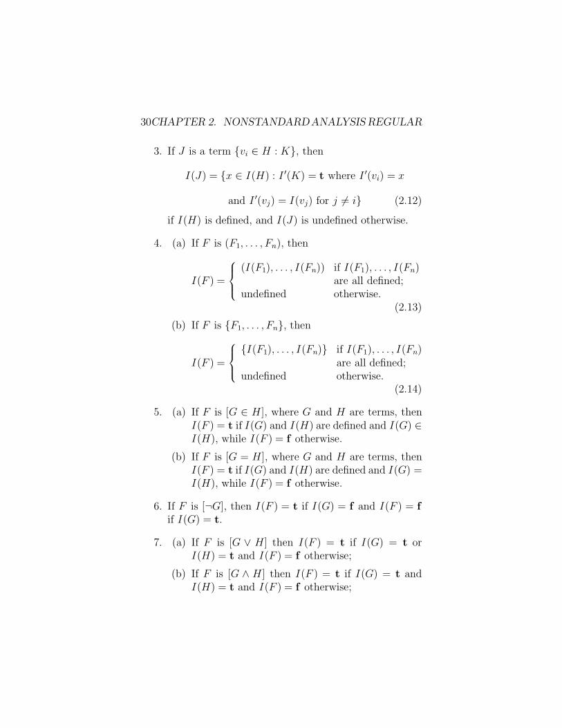
3. If J is a term {vi ∈ H : K}, then
I(J) = {x ∈ I(H) : I ′(K) = t where I ′(vi) = x
and I ′(vj) = I(vj) for j = i} (2.12)
if I(H) is defined, and I(J) is undefined otherwise.
4. (a) If F is (F1, . . . , Fn), then
I(F ) =
⎧⎪⎨⎪⎩
(I(F1), . . . , I(Fn)) if I(F1), . . . , I(Fn)are all defined;
undefined otherwise.(2.13)
(b) If F is {F1, . . . , Fn}, then
I(F ) =
⎧⎪⎨⎪⎩
{I(F1), . . . , I(Fn)} if I(F1), . . . , I(Fn)are all defined;
undefined otherwise.(2.14)
5. (a) If F is [G ∈ H], where G and H are terms, thenI(F ) = t if I(G) and I(H) are defined and I(G) ∈I(H), while I(F ) = f otherwise.
(b) If F is [G = H], where G and H are terms, thenI(F ) = t if I(G) and I(H) are defined and I(G) =I(H), while I(F ) = f otherwise.
6. If F is [¬G], then I(F ) = t if I(G) = f and I(F ) = fif I(G) = t.
7. (a) If F is [G ∨ H] then I(F ) = t if I(G) = t orI(H) = t and I(F ) = f otherwise;
(b) If F is [G ∧ H] then I(F ) = t if I(G) = t andI(H) = t and I(F ) = f otherwise;

2.4. ASSIGNING TRUTH VALUE TO FORMULAS 31
(c) If F is [G ⇒ H] then I(F ) = t if I(G) = f orI(H) = t and I(F ) = f otherwise;
(d) If F is [G ⇔ H] then I(F ) = t if I(G) = t andI(H) = t or I(G) = f and I(H) = f and I(F ) = fotherwise.
8. (a) If F is [∀vi ∈ G[H]], then I(F ) = t if I(G) isdefined and, for every x ∈ X , I ′(H) = t, whereI ′(vi) = x and I ′(vj) = I(vj) for every j = i;I(F ) = f otherwise.
(b) If F is [∃vi ∈ G[H]], then I(F ) = t if I(G) isdefined and there exists some x ∈ I(G) such thatI ′(H) = t, where I ′(vi) = x and I ′(vj) = I(vj) forevery j = i; I(F ) = f otherwise.
Remark 2.4.4 (The King of France Has a Beard) Itwould be possible, but exceedingly tedious, to restrict ourlanguage so that it is impossible to write formulas that con-tain expressions of the form f(x) where x is outside the do-main of f . We have instead taken the route of allowing themin the language, and have specified a more or less arbitraryassignment of truth value. In practice, such nonsensical for-mulas are easily spotted, and so no problems will arise. Notethat, assuming for concreteness that f : N → N, our assign-ment of truth value has the following consequences:
• I(f(π) = 0) = f .
• The formula f(π) = 0 is ambiguous. It is not an ele-ment of L.
– If it is an abbreviation for ¬[f(π) = 0], thenI(f(π) = 0) = t.
– If it is an abbreviation for (f(x), 0) ∈ C whereC = {(y, z) ∈ N2 : y = z}, then I(f(π) = 0) = f .
32CHAPTER 2. NONSTANDARDANALYSIS REGULAR
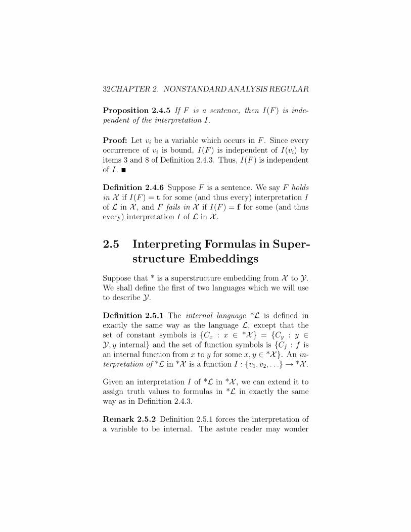
Proposition 2.4.5 If F is a sentence, then I(F ) is inde-pendent of the interpretation I.
Proof: Let vi be a variable which occurs in F . Since everyoccurrence of vi is bound, I(F ) is independent of I(vi) byitems 3 and 8 of Definition 2.4.3. Thus, I(F ) is independentof I .
Definition 2.4.6 Suppose F is a sentence. We say F holdsin X if I(F ) = t for some (and thus every) interpretation Iof L in X , and F fails in X if I(F ) = f for some (and thusevery) interpretation I of L in X .
2.5 Interpreting Formulas in Super-
structure Embeddings
Suppose that * is a superstructure embedding from X to Y.We shall define the first of two languages which we will useto describe Y.
Definition 2.5.1 The internal language *L is defined inexactly the same way as the language L, except that theset of constant symbols is {Cx : x ∈ *X} = {Cy : y ∈Y, y internal} and the set of function symbols is {Cf : f isan internal function from x to y for some x, y ∈ *X}. An in-terpretation of *L in *X is a function I : {v1, v2, . . .} → *X .
Given an interpretation I of *L in *X , we can extend it toassign truth values to formulas in *L in exactly the sameway as in Definition 2.4.3.
Remark 2.5.2 Definition 2.5.1 forces the interpretation ofa variable to be internal. The astute reader may wonder
2.6. TRANSFER PRINCIPLE 33
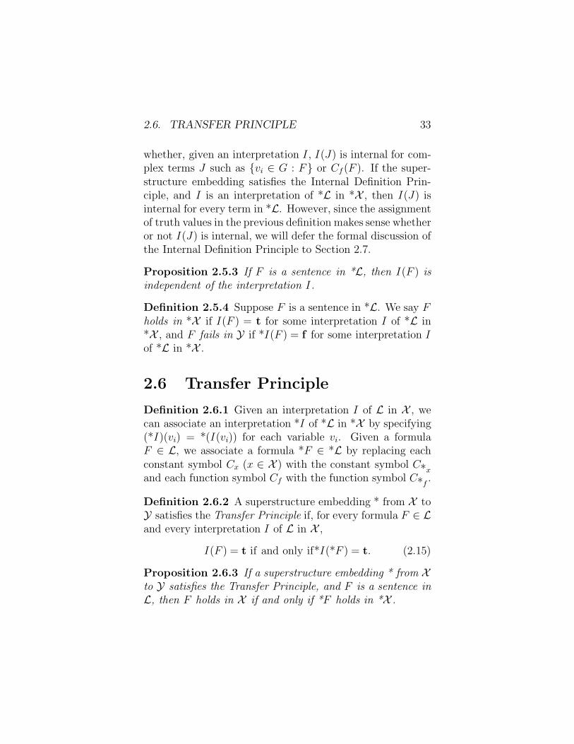
whether, given an interpretation I , I(J) is internal for com-plex terms J such as {vi ∈ G : F} or Cf (F ). If the super-structure embedding satisfies the Internal Definition Prin-ciple, and I is an interpretation of *L in *X , then I(J) isinternal for every term in *L. However, since the assignmentof truth values in the previous definition makes sense whetheror not I(J) is internal, we will defer the formal discussion ofthe Internal Definition Principle to Section 2.7.
Proposition 2.5.3 If F is a sentence in *L, then I(F ) isindependent of the interpretation I.
Definition 2.5.4 Suppose F is a sentence in *L. We say Fholds in *X if I(F ) = t for some interpretation I of *L in*X , and F fails in Y if *I(F ) = f for some interpretation Iof *L in *X .
2.6 Transfer Principle
Definition 2.6.1 Given an interpretation I of L in X , wecan associate an interpretation *I of *L in *X by specifying(*I)(vi) = *(I(vi)) for each variable vi. Given a formulaF ∈ L, we associate a formula *F ∈ *L by replacing eachconstant symbol Cx (x ∈ X ) with the constant symbol C*xand each function symbol Cf with the function symbol C*f
.
Definition 2.6.2 A superstructure embedding * from X toY satisfies the Transfer Principle if, for every formula F ∈ Land every interpretation I of L in X ,
I(F ) = t if and only if*I(*F ) = t. (2.15)
Proposition 2.6.3 If a superstructure embedding * from Xto Y satisfies the Transfer Principle, and F is a sentence inL, then F holds in X if and only if *F holds in *X .
34CHAPTER 2. NONSTANDARDANALYSIS REGULAR
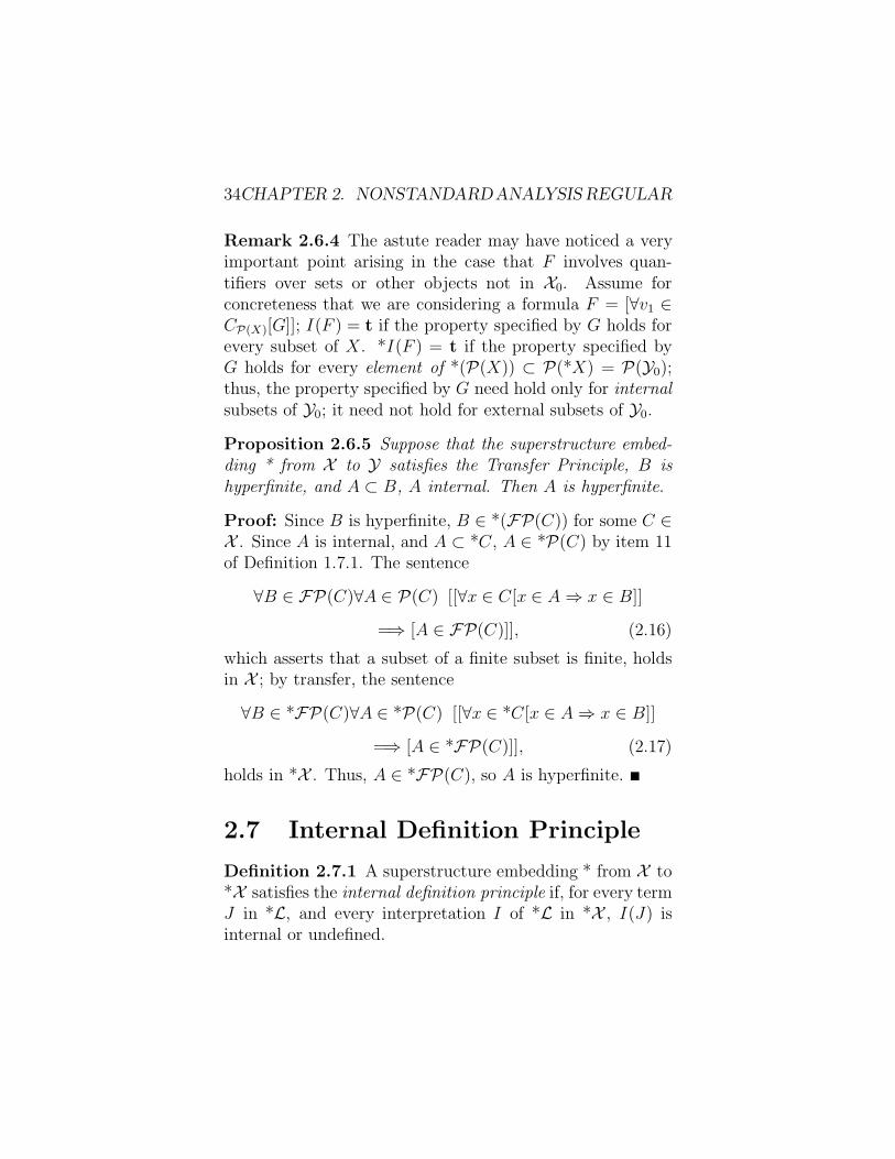
Remark 2.6.4 The astute reader may have noticed a veryimportant point arising in the case that F involves quan-tifiers over sets or other objects not in X0. Assume forconcreteness that we are considering a formula F = [∀v1 ∈CP(X)[G]]; I(F ) = t if the property specified by G holds forevery subset of X. *I(F ) = t if the property specified byG holds for every element of *(P(X)) ⊂ P(*X) = P(Y0);thus, the property specified by G need hold only for internalsubsets of Y0; it need not hold for external subsets of Y0.
Proposition 2.6.5 Suppose that the superstructure embed-ding * from X to Y satisfies the Transfer Principle, B ishyperfinite, and A ⊂ B, A internal. Then A is hyperfinite.
Proof: Since B is hyperfinite, B ∈ *(FP(C)) for some C ∈X . Since A is internal, and A ⊂ *C , A ∈ *P(C) by item 11of Definition 1.7.1. The sentence
∀B ∈ FP(C)∀A ∈ P(C) [[∀x ∈ C [x ∈ A ⇒ x ∈ B]]
=⇒ [A ∈ FP(C)]], (2.16)
which asserts that a subset of a finite subset is finite, holdsin X ; by transfer, the sentence
∀B ∈ *FP(C)∀A ∈ *P(C) [[∀x ∈ *C [x ∈ A ⇒ x ∈ B]]
=⇒ [A ∈ *FP(C)]], (2.17)
holds in *X . Thus, A ∈ *FP(C), so A is hyperfinite.
2.7 Internal Definition Principle
Definition 2.7.1 A superstructure embedding * from X to*X satisfies the internal definition principle if, for every termJ in *L, and every interpretation I of *L in *X , I(J) isinternal or undefined.
2.8. NONSTANDARD EXTENSIONS 35
2.8 Nonstandard Extensions
Definition 2.8.1 A nonstandard extension of a superstruc-ture X is a superstructure embedding *:X → Y which issaturated (Definition 1.10.1) and satisfies the Transfer Prin-ciple (Definition 2.6.1) and the Internal Definition Principle(Definition 2.7.1).
Theorem 2.8.2 Suppose * : X → Y is a nonstandard ex-tension, and N ⊂ X. Then *N \N = ∅. n ∈ *N \N ⇒ n >m for every m ∈ N.
Proof: Given m ∈ N, let Am = {n ∈ *N : n > m}. Am isinternal by the Internal Definition Principle; Am ⊃ {n ∈ N :n > m}, so Am = ∅. Given m1, . . . , mk ∈ N with k ∈ N,∩k
i=1Ami = Amax{m1,...,mk} = ∅. By Saturation ∩m∈NAm = ∅.Take any n ∈ ∩m∈NAm; then n ∈ *N, but n > m for everym ∈ N, so n ∈ *N \ N.
The sentence
∀n ∈ N ∀m ∈ N [[m < n] ∨ [m = n] ∨ [m > n]] (2.18)
holds in X ; by Transfer, the sentence
∀n ∈ *N ∀m ∈ *N [[m < n] ∨ [m = n] ∨ [m > n]] (2.19)
holds in *X . Now suppose n is any element of *N \ N, andfix m ∈ N. Since * is a superstructure embedding, m ∈ *N.Since n ∈ *N \ N, m = n. Suppose n < m. The sentence
∀n ∈ N [m < n ⇒ [n = 1 ∨ n = 2 ∨ . . . ∨ n = m − 1]](2.20)
holds in N. By Transfer, we must have n = 1 ∨ n = 2 ∨. . . ∨ n = m− 1, so n ∈ N. Accordingly, n ∈ *N \N impliesn > m for every m ∈ N.

36CHAPTER 2. NONSTANDARDANALYSIS REGULAR
Theorem 2.8.3 Suppose * : X → Y is a nonstandard ex-tension. If B ∈ X and n ∈ *N \ N, then there exists ahyperfinite set D with |D| < n such that x ∈ B ⇒ *x ∈ D.
Proof: Since n ∈ *N \ N, n > m for each m ∈ N byTheorem 2.8.2. Let Λ = B, Aλ = {D ∈ *FP(B) : *λ ∈D, |D| < n}. Aλ is internal by the Internal Definition Prin-ciple and |Λ| = |B| < |X |. Given λ1, . . . , λm with m ∈ N,{*λ1, . . . , *λm} ∈ ∩m
i=1Aλi, so the intersection is not empty.Accordingly, ∩λ∈ΛAλ = ∅ by saturation; if D is any elementof ∩λ∈ΛAλ, then D ∈ *FP(B), so D is hyperfinite, |D| < n,and D ⊃ {*x : x ∈ B}.
2.9 The External Language
We shall define a language L which permits us to refer toexternal objects, including the set of ordinary natural num-bers N, viewed as a subset of its nonstandard extension *N,or the set of all nonstandard real numbers infinitely closeto a given real number. We can use all the usual axiomsof conventional mathematics to make arguments involvingformulas in L; however, the Transfer Principle cannot beapplied to formulas in L.
Definition 2.9.1 The external language L is defined in ex-actly the same way as the language L, except that the setof constant symbols is {Cy : z ∈ Y} and the set of func-tion symbols is {Cf : f is a function from x to y for some
x, y ∈ Y}. An interpretation of L in Y is a function from{v1, v2, . . .} to Y. Given a formula F in L and such an in-terpretation I , the truth value I(F ) is defined exactly as inDefinition 2.4.3. If F is a sentence of L, we say that F holdsin Y if I(F ) = t for some interpretation of I(F ) in Y, andF fails in Y otherwise.

2.10. THE CONSERVATION PRINCIPLE 37
2.10 The Conservation Principle
The usual axiomatization of set theory is due to Zermelo andFrankel. The Zermelo-Frankel axioms, with the addition ofthe Axiom of Choice, are collectively referred to as ZFC.
Theorem 2.10.1 (Los,Robinson,Luxemburg) Let X bea superstructure in a model of ZFC. Then there exists a non-standard extension * : X → Y.
Proof: See Appendix A.
Corollary 2.10.2 (The Conservation Principle) Let Abe a set of axioms containing the axioms of ZFC. SupposeF is a sentence in L which can be deduced from A andthe assumption that there exists a nonstandard extension* : X → Y. Then F has a proof using the axioms of Aalone.

38CHAPTER 2. NONSTANDARDANALYSIS REGULAR
Chapter 3
Euclidean, Metric andTopological Spaces
In this Chapter, we explore the nonstandard formulationof the basic results in Euclidean, Metric and TopologicalSpaces. The results are due for the most part to Robinson(1966) and Luxemburg (1969). The results stated here are ofconsiderable use in applications of nonstandard analysis toeconomics. In addition, the proofs given here illustrate howthe properties of nonstandard extensions are used in writingproofs. We form a superstructure by taking X0 to be theunion of the point sets of all the spaces under consideration,and suppose that * : X → Y is a nonstandard extension.
3.1 Monads
Definition 3.1.1 Suppose (X, T ) is a topological space. Ifx ∈ X, the monad of x, denoted μ(x), is ∩x∈T∈T *T . Ify ∈ *X and y ∈ μ(x), we write y x (read “y is infinitelyclose to x”).
Definition 3.1.2 Suppose (X, d) is a metric space. If x ∈
39

40 CHAPTER 3. REAL ANALYSIS
*X, the monad of x, denoted μ(x), is {y ∈ *X : *d(x, y) 0}. If x, y ∈ *X and y ∈ μ(x), we write y x (read “y isinfinitely close to x”).
Proposition 3.1.3 Suppose (X, d) is a metric space, andx ∈ X. Then the monad of x (viewing X as a metric space)equals the monad of x (viewing X as a topological space).
Proof: Suppose y is in the metric monad of x. Then *d(x, y) 0. Suppose x ∈ T ∈ T . Then there exists δ ∈ R++ such thatthe formula
d(z, x) < δ ⇒ z ∈ T (3.1)
holds in X . By Transfer,
*d(z, x) < δ ⇒ z ∈ *T (3.2)
holds in *X . Since this holds for each T satisfying x ∈ T ∈ T ,y is in the topological monad of x.
Conversely, suppose y is in the topological monad of x.Choose δ ∈ R++ and let T = {z ∈ X : d(z, x) < δ}. x ∈T ∈ T , so y ∈ *T . Therefore, *d(x, y) < δ for each δ ∈ R++,so *d(x, y) 0. Thus, y is in the metric monad of x.
Remark 3.1.4 The topological monad of x can be definedfor an arbitrary x ∈ *X, not just for x ∈ X. However, it isnot very well behaved.
Proposition 3.1.5 (Overspill) Suppose (X, T ) is a topo-logical space, x ∈ X, and A is an internal subset of *X.
1. If x ∈ A ⊂ μ(x), there exists S ∈ *T with A ⊂ S ⊂μ(x).
2. If A ⊃ μ(x), then A ⊃ *T for some T satisfying x ∈T ∈ T .
3.1. MONADS 41
3. If (X, T ) is a T1 space and μ(x) is internal, then μ(x) ={x} ∈ T .
Proof: Let T ′ = {T ∈ T : x ∈ T}.(1)Suppose A ⊂ μ(x). By Theorem 1.13.4, there exists a
hyperfinite set S ⊂ *T ′ such that T ∈ T ′ implies *T ∈ S.Let S ′ = {T ∈ S : T ⊃ A}; S ′ is internal by the InternalDefinition Principle, and hyperfinite by Proposition 1.13.5.Let S = ∩T∈S′T . Then A ⊂ S ⊂ μ(x). Since T is closedunder finite intersections, *T is closed under hyperfinite in-tersections, by Transfer. Therefore S ∈ *T .
(2) Suppose A ⊃ μ(x). Given T ∈ T ′, let AT = *T \ A.AT is internal by the Internal Definition Principle. ∩T∈T ′AT =(∩T∈T ′*T ) \ A = μ(x) \ A = ∅. By Saturation, there existT1, . . . , Tn (n ∈ N) such that ∩n
i=1ATi = ∅, so A ⊃ ∩ni=1*Ti =
*(∩ni=1Ti). Since x ∈ ∩n
i=1Ti ∈ T , the proof of (2) is com-plete.
(3) Suppose μ(x) is internal and (X, T ) is a T1 space.By (2), there exists T ∈ *T such that μ(x) ⊂ *T ⊂ μ(x),so μ(x) = *T . If y ∈ X, y = x, then there exists S ∈ Twith x ∈ S and y ∈ S. By Transfer, y ∈ *S, so y ∈ μ(x) =*T . By Transfer, y ∈ T . Since y is an arbitrary element ofX different from x, T = {x}. Then μ(x) = *T = {x} byTransfer.
Proposition 3.1.6 (Overspill) Suppose A is an internalsubset of *N.
1. If A ⊃ *N \ N, then A ⊃ {n, n + 1, . . .} for somen ∈ N.
2. If A ⊃ N, then A ⊃ {1, 2, . . . , n} for some n ∈ *N\N.
Proof: We could prove this as a corollary of Proposition3.1.5 by considering X = N ∩ {∞} with the one-point com-pactification metric. However, we shall present a direct proof.
42 CHAPTER 3. REAL ANALYSIS
Every nonempty subset of N has a first element; by transfer,every nonempty internal subset of *N has a first element.
(1) Let B = {n ∈ *N : ∀m ∈ *N[m ≥ n ⇒ m ∈ A]}.B is internal by the Internal Definition Principle. Let n bethe first element of B. Since A ⊃ *N \ N, B ⊃ *N \ N, son ∈ N.
(2) Let B = {n ∈ *N : ∀m ∈ *N[m ≤ n ⇒ m ∈ A]}. Band *N \B are internal by the Internal Definition Principle.If *N \ B = ∅, we are done. Otherwise, let n be the firstelement of *N \ B. Since A ⊃ N, B ⊃ N, so n ∈ *N \ N.
Proposition 3.1.7 Suppose (X, T ) is a topological space.Then X is Hausdorff if and only if for every every x, y ∈ Xwith x = y, μ(x) ∩ μ(y) = ∅.
Proof: Suppose X is Hausdorff. If x, y ∈ X and x = y, wemay find S, T with x ∈ S ∈ T , y ∈ T ∈ T , and S ∩ T = ∅.*S∩*T = *(S∩T ) = ∅, by Transfer. μ(x)∩μ(y) ⊂ *S∩*T =∅.
Comversely, suppose μ(x) ∩ μ(y) = ∅. By Proposition3.1.5, we may find S, T ∈ *T with x ∈ S ⊂ μ(x) and y ∈T ⊂ μ(y), and thus S ∩ T = ∅. Thus, the sentence
∃S ∈ *T ∃T ∈ *T [x ∈ S ∧ y ∈ T ∧ S ∩ T = ∅] (3.3)
holds in *X . By Transfer, the sentence
∃S ∈ T ∃T ∈ T [x ∈ S ∧ y ∈ T ∧ S ∩ T = ∅] (3.4)
holds in X , so X is Hausdorff.
Definition 3.1.8 If (X, T ) is a Hausdorff space, y ∈ *X,and y ∈ μ(x), we write x = ◦y (read “x is the standard partof y”).

3.1. MONADS 43
Proposition 3.1.9 Suppose {xn : n ∈ *N} is an internalsequence of elements of *R. Then the standard sequence{◦xn : n ∈ N} converges to x ∈ R if and only if there existsn0 ∈ *N \N such that xn x for every n ≤ n0, n ∈ *N \N.
Proof: Suppose ◦xn converges to x. Fix δ ∈ R++. Thereexists nδ ∈ N such that n ≥ nδ, n ∈ N implies |◦xn − x| <δ/2; thus, |xn − x| < δ. Thus, given δ ∈ R++ and k ∈ N,let Aδk = {n ∈ *N : n ≥ k and |xm − x| < δ for each m ∈{k, . . . , n}}. For any finite collection {(δ1, k1), . . . (δn, kn)}with ki ≥ nδi, ∩n
i=1Aδiki = ∅. Let Λ = {(δ, k) ∈ R++ ×N : k ≥ nδ}. By Saturation, ∩(δ,k)∈ΛAδk = ∅. Choosen0 ∈ ∩(δ,k)∈ΛAδk. Then n0 ∈ *N \N; given n ∈ *N \N withn ≤ n0, |xn − x| 0.
Conversely, suppose there exists n0 ∈ *N \ N such thatn ∈ *N, n ≤ n0 implies xn x. Given δ ∈ R++, letA = {n ∈ *N : |xn − x| < δ/2} ∪ {n ∈ *N : n > n0}.A is internal and contains *N \ N. By Proposition 3.1.6,A ⊃ {n, n + 1, . . .} for some n ∈ N. Thus, |◦xm − x| < δ form ∈ N satisfying m ≥ n. Therefore ◦xn converges to x.
Proposition 3.1.10 Suppose {xn : n ∈ N} is a sequence ofelements of R. Then xn → x ∈ R if and only if xn x forevery n ∈ *N \ N.
Proof: Suppose xn → x. Given ε ∈ R++, there existsn0 ∈ N such that the sentence
∀n ∈ N[n ≥ n0 ⇒ |xn − x| < ε] (3.5)
holds in X . By Transfer, the sentence
∀n ∈ *N[n ≥ n0 ⇒ |xn − x| < ε] (3.6)
holds in *X . If n ∈ *N \ N, then |xn − x| < ε; since ε is anarbitrary element of R++, xn x.
Conversely, suppose xn x for all n ∈ *N \ N. Forn ∈ N, ◦xn = xn, so xn → x by Proposition 3.1.9.
44 CHAPTER 3. REAL ANALYSIS
3.2 Open and Closed Sets
Proposition 3.2.1 Suppose (X, T ) is a topological space.Then A ⊂ X is open if and only if μ(x) ⊂ *A for everyx ∈ A.
Proof: If A is open and x ∈ A, then μ(x) ⊂ *A by Definition3.1.1. Conversely, suppose μ(x) ⊂ *A for every x ∈ A. ByProposition 3.1.5, we may find S ∈ *T with x ∈ S ⊂ μ(x).Thus, the sentence
∃S ∈ *T x ∈ S ⊂ *A (3.7)
holds in *X , so the sentence
∃S ∈ T x ∈ S ⊂ A (3.8)
holds in X by Transfer. Thus, A is open.
Proposition 3.2.2 Suppose (X, T ) is a topological space.Then A ⊂ X is closed if and only if y ∈ *A implies x ∈ Afor every x ∈ X such that y ∈ μ(x).
Proof: Let B = X \ A.Suppose A is closed. If y ∈ *A and y ∈ μ(x) with x ∈ X\
A, then x ∈ B. Since A is closed, B is open. Since y ∈ μ(x),y ∈ *B by Proposition 3.2.1. *B ∩ *A = *(B ∩ A) = ∅, byTransfer. Thus, y ∈ *A, a contradiction.
Conversely, suppose y ∈ *A implies x ∈ A for everyx ∈ X such that y ∈ μ(x). Suppose x ∈ B. Then we musthave y ∈ *X \ *A = *B for every y ∈ μ(x). Accordingly, Bis open by Proposition 3.2.1, so A is closed.
Proposition 3.2.3 Suppose(X, T ) is a topological space, andA ⊂ *X is internal. Then {x ∈ X : ∃y ∈ A [y ∈ μ(x)]} isclosed.
3.3. COMPACTNESS 45
Proof: Let C = {x ∈ X : ∃y ∈ A [y ∈ μ(x)]}; we shall showthat B = X \ C is open. Let D = *X \ A; D is internal bythe Internal Definition Principle. If x ∈ B, then D ⊃ μ(x),so D ⊃ *T for some T satisfying x ∈ T ∈ T , by Proposition3.1.5. If y ∈ T , then μ(y) ⊂ *T , so D ⊃ μ(y), so y ∈ B.Thus, B is open, so C is closed.
3.3 Compactness
Definition 3.3.1 Let (X, T ) be a topological space and y ∈*X. We say y is nearstandard if there exists x ∈ X such thaty x. We let ns(*X) denote the set of nearstandard pointsin *X.
Theorem 3.3.2 Let (X, T ) be a topological space. Then(X, T ) is compact if and only if every y ∈ *X is nearstan-dard.
Proof: Suppose (X, T ) is compact, and there is some y ∈*X which is not nearstandard. Then for every x ∈ X, thereexists Tx with x ∈ Tx ∈ T and y ∈ *Tx. {Tx : x ∈ X}is thus an open cover of X; let {Tx1, . . . , Txn} be a finitesubcover (so n ∈ N). Since * is a superstructure embedding,∪n
i=1*Txi = *(∪ni=1Txi) = *X, so y ∈ *X, a contradiction.
Conversely, suppose that every y ∈ *X is nearstandard.Let {Tλ : λ ∈ Λ} be an open cover of X. Let Cλ =X \ Tλ. If there is no finite subcover, then for every col-lection {λ1, . . . , λn} with n ∈ N, ∩n
i=1Cλi = ∅. ∩ni=1*Cλi =
*(∩ni=1Cλi) = ∅. |Λ| ≤ |X1|, so by saturation, C = ∩λ∈Λ*Cλ =
∅. Choose any y ∈ C . Given x ∈ X, there exists λ such thatx ∈ Tλ. Since y ∈ C ⊂ *Cλ, y ∈ *Tλ, so y x. Since x isan arbitrary element of X, y is not nearstandard, a contra-diction. Thus, {Tλ : λ ∈ Λ} has a finite subcover, so X iscompact.

46 CHAPTER 3. REAL ANALYSIS
Definition 3.3.3 x ∈ *R is said to be finite if there is somen ∈ N such that x ≤ n.
Proposition 3.3.4 Suppose y ∈ *R, and y is finite. Theny is nearstandard.
Proof: Let A = {z ∈ R : z < y}, x = sup A. Givenδ ∈ R++, we can find z ∈ A with z > x − δ. But z < y, sox− δ < y. On the other hand, x+ δ > y by the definitions ofA and x. Therefore x−δ < y < x+δ. Since δ is an arbitraryelement of R++, y x, so y is nearstandard.
Theorem 3.3.5 (Bolzano-Weierstrass) If C is a closedand bounded subset of Rk (k ∈ N), then C is compact.
Proof: Suppose y ∈ *C . Since C is bounded, there existsn ∈ N such that
∀z ∈ C|z| ≤ n. (3.9)
By Transfer
∀z ∈ *C|z| ≤ n (3.10)
and so each component yi of y is finite. By Proposition3.3.4, yi is nearstandard, with yi xi for some xi ∈ R. Letx = (x1, . . . , xk). Then y x. Since C is closed, x ∈ C .Thus, C is compact by Theorem 3.3.2.
Theorem 3.3.6 Suppose � is a binary relation on a com-pact toplogical space (X, T ) satisfying
1. irreflexivity (for all x ∈ X, x � x);
2. transitivity (for all x, y, z ∈ X, x � y, y � z ⇒ x �z);
3. continuity ({(x, y) ∈ X2 : x � y} is open).
3.3. COMPACTNESS 47
Then X contains a maximal element with respect to �, i.e.there is some x ∈ X such that there is no z ∈ X with z � x.
Proof: By Theorem 1.13.4, there exists a hyperfinite set Asuch that T ∈ T ⇒ ∃x ∈ A [x ∈ *T ]. Since � is irreflexiveand transitive, any finite set B ⊂ X contains a maximalelement with respect to �. By Transfer, any hyperfinite setcontains a maximal element with respect to *�. Let y besuch a maximal element of A. Since X is compact, thereexists x ∈ X such that y x by Theorem 3.3.2.
Suppose z ∈ X and z � x. Then there exists S, T withx ∈ T ∈ T and z ∈ S ∈ T such that v � w for eachv ∈ S and w ∈ T . By transfer, v*�w for each v ∈ *S andeach w ∈ *T . But there exists v ∈ *S ∩ A, and so v*�y, acontradiction. Thus, x is maximal in X with respect to �.
Proposition 3.3.7 Suppose(X, T ) is a regular topologicalspace, and A ⊂ *X is internal. Suppose further that everyy ∈ A is nearstandard. Then {x ∈ X : ∃y ∈ A [y ∈ μ(x)]}is compact.
Proof: Let C = {x ∈ X : ∃y ∈ A [y ∈ μ(x)]}. Sup-pose {Cλ : λ ∈ Λ} is a collection of relatively closed subsetsof C , with ∩λ∈ΛCλ = ∅, but ∩n
i=1Cλi = ∅ for every finitecollection {λ1, . . . , λn}; C is closed by Proposition 3.2.3, soCλ is closed in X. Given x ∈ C with x ∈ Cλ, we mayfind sets Sλx, Tλx ∈ T such that Cλ ⊂ Sλx, x ∈ Tλx, andSλx ∩ Tλx = ∅. Let Λ′ = {(λ, x) : x ∈ Cλ}. Given any fi-nite collection {(λ1, x1), . . . , (λn, xn)} ⊂ Λ′, ∩n
i=1Sλixi is anopen set; because it contains ∩n
i=1Cλi = ∅, it is not empty.Choose c ∈ ∩n
i=1Cλi. Then c ∈ C , so there exists a ∈ Awith a ∈ μ(c). ∩n
i=1*Sλixi = * ∩ni=1 Sλixi ⊃ μ(c) by Proposi-
tion 3.2.1. Therefore, A ∩ (∩ni=1*Sλixi) = ∅. By saturation,
A ∩ (∩(λ,x)∈Λ′*Sλixi) = ∅; choose y ∈ A ∩ (∩(λ,x)∈Λ′*Sλixi).
48 CHAPTER 3. REAL ANALYSIS
Since y ∈ A, y is nearstandard, so y ∈ μ(x) for some x ∈ X.By the definition of C , x ∈ C . Since ∩λ∈ΛCλ = ∅, thereexists λ ∈ Λ with x ∈ λ. Since *Tλx ⊃ μ(x), *Sλx ∩ *Tλx =*(Sλx ∩ Tλx) = ∅, we get y ∈ μ(x), a contradiction. There-fore, C is compact.
3.4 Products
Proposition 3.4.1 Let (Xλ, Tλ) be a family of topologicalspaces, and let (X, T ) be the product topological space. Then
*X = {y : y is an internal function from *Λ to ∪λ∈*Λ
*Xλ
and ∀λ ∈ *Λ yλ ∈ *Xλ}. (3.11)
Given x ∈ X,
μ(x) = {y ∈ *X : ∀λ ∈ Λ yλ xλ}. (3.12)
Proof: The formal definition of the product is
X = {f ∈ F(Λ,∪λ∈ΛXλ) : ∀λ ∈ Λ f(λ) ∈ Xλ} (3.13)
where F(A, B) denotes the set of all functions from A to B.By the Transfer Principle,
*X = {f ∈ *(F(Λ,∪λ∈ΛXλ)) : ∀λ ∈ *Λ f(λ) ∈ *Xλ}(3.14)
= {y : *Λ → ∪λ∈*Λ
*Xλ : y is internal, ∀λ ∈ *Λ yλ ∈ *Xλ}.(3.15)
Suppose y ∈ μ(x) with x ∈ X. Fix λ ∈ Λ. Given T ∈ Tλ
with xλ ∈ T , let S = {z ∈ X : zλ ∈ T}. S ∈ T and x ∈ S,so y ∈ *S. Therefore, yλ ∈ *T , so yλ xλ.
Conversely, suppose y ∈ *X and yλ xλ for all λ ∈ Λ. Ifx ∈ T ∈ T , then there exist λ1, . . . , λn ∈ Λ with n ∈ N and
3.5. CONTINUITY 49
Tλi ∈ Ti such that if S = {z ∈ X : zλi ∈ Tλi(1 ≤ i ≤ n)},then x ∈ S ⊂ T . But *S = {z ∈ *X : zλi ∈ *Tλi(1 ≤ i ≤ n})by Transfer, so y ∈ *S ⊂ *T . Therefore y x.
Theorem 3.4.2 (Tychonoff) Let (Xλ, Tλ) (λ ∈ Λ) be afamily of topological spaces, and (X, T ) the product topologi-cal space. If (Xλ, Tλ) is compact for each λ ∈ Λ, then (X, T )is compact.
Proof: Suppose y ∈ *X. For each λ ∈ Λ, there existsxλ ∈ Xλ such that yλ xλ. By the Axiom of Choice, thisdefines an element x ∈ X such that yλ xλ for each λ ∈ Λ.Therefore, y x by Proposition 3.4.1. Thus, every y ∈ *Xis nearstandard, so X is compact by Theorem 3.3.2.
3.5 Continuity
Proposition 3.5.1 Suppose (X,S) and (Y, T ) are topologi-cal spaces and f : X → Y . Then f is continuous if and onlyif *f(μ(x)) ⊂ μ(f(x)) for every x ∈ X.
Proof: Suppose f is continuous. If y = f(x) and y ∈ T ∈ T ,then S = f−1(T ) ∈ S. Hence, the sentence ∀z ∈ S f(z) ∈ Tholds in X . By Transfer, the sentence ∀z ∈ *S *f(z) ∈ *Tholds in *X . If z ∈ μ(x), then z ∈ *S, so *f(z) ∈ *T . Sincethis holds for every T satisfying f(x) ∈ T ∈ T , *f(z) ∈μ(f(x)). Thus, *f(μ(x)) ⊂ μ(f(x)).
Conversely, suppose *f(μ(x)) ⊂ μ(f(x)) for every x ∈ X.Choose T such that f(x) ∈ T ∈ T . By Proposition 3.1.5, wemay find S ∈ *S such that x ∈ S ⊂ μ(x). Accordingly, thesentence
∃S ∈ *S [x ∈ S ∧ *f(S) ⊂ *T ] (3.16)
holds in *X ; by Transfer, the sentence
∃S ∈ S [x ∈ S ∧ f(S) ⊂ T ] (3.17)

50 CHAPTER 3. REAL ANALYSIS
holds in X , so f is continuous.
Corollary 3.5.2 If f : R → R, then f is continuous if andonly if y x ∈ R implies *f(y) f(x).
Definition 3.5.3 Suppose (X,S) and (Y, T ) are topologicalspaces with (Y, T ) Hausdorff, and suppose f : *X → *Y isinternal. f is said to be S-continuous if f(x) is nearstandardand f(μ(x)) ⊂ μ(◦f(x)) for every x ∈ X.
Definition 3.5.4 A topological space (X, T ) is regular if itis Hausdorff and, given x ∈ X and C ⊂ X with x ∈ C andC closed, there exist S, T ∈ T with x ∈ S, C ⊂ T , andS ∩ T = ∅.
Proposition 3.5.5 Suppose (X,S) and (Y, T ) are topolog-ical spaces with (Y, T ) regular, and f : *X → *Y is S-continuous. Define ◦f : X → Y by (◦f)(x) = ◦(f(x)) foreach x ∈ X. Then ◦f is a continuous function.
Proof: Because f(x) is nearstandard for each x ∈ X, thereexists y ∈ Y such that f(x) ∈ μ(y); since (Y, T ) is Hausdorff,this y is unique by Proposition 3.1.7. Thus, the formula for◦f defines a function.
Suppose x ∈ X, y = ◦f(x). If y ∈ V ∈ T , then X \V is closed. Since (Y, T ) is regular, we may find S, T ∈T with y ∈ S, X \ V ⊂ T , and S ∩ T = ∅. Since f isS-continuous, f−1(*S) ⊃ μ(x). f−1(*S) is internal by theInternal Definition Principle, so it contains *W for some Wsatisfying x ∈ W ∈ S, by Proposition 3.1.5. If w ∈ W ,then w ∈ *W , so f(w) ∈ *S. If ◦f(w) ∈ V , then ◦f(w) ∈X \ V ⊂ T . Since T ∈ T , f(w) ∈ *T by Proposition 3.2.1.But *S ∩ *T = *(S ∩ T ) = ∅, so f(w) ∈ *S, a contradictionwhich shows ◦f(w) ∈ V for w ∈ W . Thus, ◦f is continuous.
3.5. CONTINUITY 51
Remark 3.5.6 In the proof of Proposition 3.5.5, one is temptedto consider the function g = *(◦f) and apply Proposition3.5.1. However, since ◦f is constructed using the nonstan-dard extension, using the properties of f propels us intoa second nonstandard extension *(*X ), creating more prob-lems than we solve. Hence, the argument must proceed with-out invoking the nonstandard characterization of continuitypresented in Proposition 3.5.1.
Definition 3.5.7 Suppose (X, T ) is a topological space and(Y, d) is a metric space. A function f : X → Y is bounded ifsupx,y∈X d(f(x), f(y)) < ∞. (C(X, Y ), d) denotes the metricspace of bounded continuous functions from X to Y , whered(f, g) = supx∈X d(f(x), g(x)).
Theorem 3.5.8 (Nonstandard Ascoli’s Theorem)Let (X, T ) be a compact topological space and (Y, d) a met-
ric space. If f is an S-continuous function from *X to *Y ,then *d(f, ◦f) 0, i.e. f is nearstandard as an element of*(C(X, Y ), d), and ◦f is its standard part.
Proof: By Proposition 3.5.5, ◦f is a continuous functionfrom (X, T ) to (Y, d). Let g = ◦f . Given z ∈ *X, z ∈ μ(x)for some x ∈ X. Transferring the triangle inequality,
*d(*g(z), f(z)) ≤
*d(*g(z), g(x)) + *d(g(x), f(x)) + *d(f(x), f(z)).(3.18)
The first term is infinitesimal by Propositions 3.5.1 and 3.5.5;the second by the definition of g = ◦f ; and the third becausef is S-continuous. Therefore *d(g(z), f(z)) 0 for everyz ∈ *X. Therefore, *d(f, g) < ε for every ε ∈ R++, and thus*d(f, g) 0.

52 CHAPTER 3. REAL ANALYSIS
Corollary 3.5.9 (Ascoli) Suppose A ⊂ C([0, 1],R) isclosed, bounded and equicontinuous. Then A is compact.
Proof: Given ε ∈ R++, there exists δ ∈ R++ and M ∈ Rsuch that the sentence
∀f ∈ A ∀x, y ∈ [0, 1] [[|f(x)| < M ]
∧ [|y − x| < δ ⇒ |f(x) − f(y)| < ε]] (3.19)
holds in X . By Transfer, the sentence
∀f ∈ *A ∀x, y ∈ *[0, 1] [[|f(x)| < M ]
∧ [|y − x| < δ ⇒ |*f(x) − *f(y)| < ε]] (3.20)
holds in *X . Suppose f ∈ *A. f(x) is finite for all x ∈ *[0, 1].Moreover, if y ∈ μ(x), then |f(y) − f(x)| < ε; since ε isarbitrary, |f(y) − f(x)| 0. Therefore *f is S-continuous,so f ∈ μ(◦f). Since A is closed, ◦f ∈ A by Proposition3.2.2. Thus, every element f ∈ *A is nearstandard, so A iscompact by Theorem 3.3.2.
3.6 Differentiation
Definition 3.6.1 Suppose x, y ∈ *R. We write y = o(x) ifthere is some δ 0 such that |y| ≤ δ|x| and y = O(x) ifthere is some m ∈ N such that |y| ≤ M |x|.
Proposition 3.6.2 Suppose f : Rm → Rn and x ∈ Rm.Then f is differentiable at x if and only if there exists alinear function J : Rm → Rn such that *f(y) = f(x) +*J(y − x) + o(y − x) for all y x.
3.7. RIEMANN INTEGRATION 53
Proof: Let L be the set of all linear maps from Rm to Rn.Suppose f is differentiable at x. Then there exists J ∈ Lsuch that for each ε ∈ R++, there exists δ ∈ R++ such thatthe sentence
∀y ∈ Rm[|y − x| < δ ⇒ |f(y) − f(x) − J(y − x)| ≤ ε|y − x|](3.21)
holds in X ; by Transfer, the setence
∀y ∈ *Rm [|y−x| < δ ⇒ |f(y)−f(x)−*J(y−x)| ≤ ε|y−x|](3.22)
holds in *X . Therefore, if y x, then |f(y)− f(x)− *J(y−x)| ≤ ε|y − x|. Since ε is an arbitrary element of R++,|f(y) − f(x) − *J(y − x)| = o(|y − x|) for all y x.
Conversely, suppose that there exists J ∈ L such thaty x implies |f(y) − f(x) − *J(y − x)| = o(|y − x|). Fixε ∈ R++. Then the sentence
∃δ ∈ *R++ [|y − x| < δ
⇒ |f(y)− f(x) − *J(y − x)| ≤ ε|y − x|] (3.23)
holds in *X . By Transfer, the sentence
∃δ ∈ R++ [|y − x| < δ
⇒ |f(y) − f(x) − J(y − x)| ≤ ε|y − x|] (3.24)
holds in X . Since ε is an arbitrary element of R++, f isdifferentiable at x.
3.7 Riemann Integration
Theorem 3.7.1 Suppose [a, b] ⊂ R and f : [a, b] → R iscontinuous. Given n ∈ *N \ N,∫ b
af(t)dt = ◦
(1
n
n∑k=1
*f(a +k(b − a)
n)
). (3.25)

54 CHAPTER 3. REAL ANALYSIS
Proof: Let In = 1n
∑nk=1 f(a + k(b−a)
n) for n ∈ N. By Trans-
fer, In = 1n
∑nk=1 *f(a+k(b−a)
n) for n ∈ *N. Since f is continu-
ous, In → ∫ ba f(t)dt. By Proposition 3.1.10, *In ∫ b
t=a f(t)dtfor all n ∈ *N \ N.
3.8 Differential Equations
Nonstandard analysis permits the construction of solutionsof ordinary differential equations by means of a hyperfinitepolygonal approximation; the standard part of the polygonalapproximation is a solution of the differential equation.
Construction 3.8.1 Suppose F : Rk × [0, 1] → Rk is con-tinuous, there exists M ∈ N such that |F (x, t)| ≤ M for all(x, t) ∈ Rk × [0, 1], and y0 ∈ Rk. Choose n ∈ *N \ N. Bythe Transfer Principle, we can define inductively
z(
0n
)= y0
z(
k+1n
)= z
(kn
)+ 1
n*F
(z(
kn
), k
n
) (3.26)
and then extend z to a function with domain *[0, 1] by linearinterpolation
z(t) = ([nt]+1−nt)z
([nt]
n
)+(nt−[nt])z
([nt] + 1
n
)(3.27)
where [nt] denotes the greatest (nonstandard) integer lessthan or equal to nt. Let
y(t) = ◦(z(t)) for z ∈ [0, 1]. (3.28)
Theorem 3.8.2 With the notation in Construction 3.8.1, zis S-continuous and y is a solution of the ordinary differentialequation
y(0) = yo
y′(t) = F (y(t), t).(3.29)
3.8. DIFFERENTIAL EQUATIONS 55
Proof: Given r, s ∈ *[0, 1] with r s, |z(r) − z(s)| ≤M |r − s| 0, so z is S-continuous. By Theorem 3.5.8, y iscontinuous and there exists δ 0 such that |z(t)−*y(t)| ≤ δfor all t ∈ *[0, 1]. Then
y(t)− y0 z(t) − z(0) ∑[nt]−1k=0
(z(
k+1n
)− z
(kn
))
=∑[nt]−1
k=01n*F
(z(
kn
), k
n
) ∑[nt]−1
k=01n*F
(*y(
kn
), k
n
)
∫ t0 F (y(s), s)ds
(3.30)by Theorem 3.7.1. Since y(t)−y0 and
∫ t0 F (y(s), s)ds are both
standard, they are equal. By the Fundamental Theorem ofCalculus, y′(t) = F (y(t), t) for all t ∈ [0, 1], so y is a solutionof the ordinary differential equation 3.29.

56 CHAPTER 3. REAL ANALYSIS
Chapter 4
Loeb Measure
The Loeb measure was developed originally by Peter Loeb(1975) to solve a problem in potential theory. Loeb’s con-struction allows one to convert nonstandard summations onhyperfinite spaces to measures in the usual standard sense.It has been used very widely in probability theory, and is animportant tool in nonstandard mathematical economics.
4.1 Existence of Loeb Measure
Definition 4.1.1 An internal probability space is a triple(A,A, ν) where
1. A is an internal set,
2. A ⊂ (*P)(A) is an internal σ-algebra, i.e.
(a) A ∈ A;
(b) B ∈ A implies A \ B ∈ A; and
(c) If {Bn : n ∈ *N} is an internal sequence withBn ∈ A, then ∩
n∈*NBn ∈ A and ∪
n∈*NBn ∈ A;
and
57
58 CHAPTER 4. LOEB MEASURE
3. ν : A → *[0, 1] is an internal *-countably additiveprobability measure, i.e.
(a) ν(A) = 1; and
(b) if {Bn : n ∈ *N} is an internal sequence and Bn∩Bm = ∅ whenever n = m, then ν(∪
n∈*NBn) =∑
n∈*Nν(Bn).
Remark 4.1.2 The Loeb measure construction also worksif we merely assume that A is closed under finite unions andν is finitely additive. We shall be primarily interested inhyperfinite spaces, in which integration is just summation.
Definition 4.1.3 An internal probability space is hyperfi-nite if A is a hyperfinite set, A = (*P)(A) (i.e. A is the classof all internal subsets of A), and there is an internal set ofprobability weights {λa : a ∈ A} such that ν(B) =
∑a∈B λa
for all B ∈ A.
Example 4.1.4 The canonical example of a hyperfinite prob-ability space is (A,A, ν), where A = {1, . . . , n} for some
n ∈ *N \ N, A = (*P)(A), and ν(B) = |B|n
for all B ∈ A.
Construction 4.1.5 (Loeb Measure) Suppose (A,A, ν)is an internal probability space. The Loeb measure con-struction creates an (external) probability measure in thestandard sense, defined on an (external) σ-algebra of (inter-nal and external) subsets of the internal set A. Define
A = {B ⊂ A : ∀ε ∈ R++ ∃C ∈ A ∃D ∈ A
[C ⊂ B ⊂ D, ν(D \ C) < ε]} (4.1)
andν(B) = inf{◦ν(D) : B ⊂ D ∈ A}
= sup{◦ν(C) : C ⊂ B, C ∈ A} (4.2)
for B ∈ A. ν is called the Loeb measure generated by ν.

4.1. EXISTENCE OF LOEB MEASURE 59
Theorem 4.1.6 (Loeb) Suppose (A,A, ν) is an internal prob-ability space. Then
1. A is a σ-algebra, A ⊃ A;
2. ν is a countably additive probability measure;
3. A is complete with respect to ν;
4. ν(B) = ◦ν(B) for every B ∈ A; and
5. for each B ∈ A, there exists A ∈ A such that
ν((A \ B) ∪ (B \ A)) = 0. (4.3)
Proof:
1. First, we note that part 4 is obvious.
2. Second, we prove part 5. If B ∈ A, then for eachn ∈ N, we may find Cn, Dn ∈ A with C1 ⊂ C2 ⊂ . . . ⊂B . . . D2 ⊂ D1 and ν(Dn \ Cn) < 1/n. By Theorem1.10.3, we can extend Cn andDn to internal sequencesin A. {n ∈ *N : [Cm ⊂ Cm+1 ⊂ Dm+1 ⊂ Dm ∧ν(Dm \Cm) < 1/m] (1 ≤ m ≤ n)} is internal and con-tains N, so it contains some n ∈ *N\N by Proposition3.1.6. Cn ∈ A. If m ∈ N, ν((Cn \ B) ∪ (B \ Cn)) ≤ν((Cn\Cm)∪(Dm\Cn)) ≤ ν(Dm\Cm) < 1/m. Since mis an arbitrary element of N, ν((Cn\B)∪(B\Cn)) = 0.
3. Next, we establish parts 1 and 2.
(a) Suppose B, B ′ ∈ A. Fix ε ∈ R++, and find C ⊂B ⊂ D, C ′ ⊂ B ′ ⊂ D′ with C, C ′, D, D′ ∈ A andν(D\C) < ε/2, ν(D′\C ′) < ε/2. C\D′ ⊂ B\B ′ ⊂D \C ′ and ((D \C ′)\ (C \D′)) ⊂ ((D \C)∪ (D′ \C ′)), so ν((D \ C ′) \ (C \ D′)) < ε/2 + ε/2 = ε.Thus, B \ B ′ ∈ A.
60 CHAPTER 4. LOEB MEASURE
(b) Now suppose B1, B2, . . . ∈ A and let B = ∪n∈NBn.By considering B ′
n = Bn \ ∪n−1i=1 Bi, we may as-
sume without loss of generality that the Bi’s aredisjoint. Given ε ∈ R++, we may find Cn ⊂ Bn ⊂Dn with Cn, Dn ∈ A satisfying ν(Dn \ Cn) <ε/2n+1. Extend Cn and Dn to internal sequenceswith Cn, Dn ∈ A by Theorem 1.10.3. If we letαn = ◦(ν(∪n
i=1Ci)), then αn is a nondecreasing se-quence in [0, 1], so it converges to some α ∈ R. ByProposition 3.1.9, we may find some n0 ∈ *N \Nsuch that ν(∪n
i=1Ci) α for n ∈ *N \N, n ≤ n0.Moreover, {n : ν(∪n
i=1Di) ≤ ν(∪ni=1Ci)+ε/2} is an
internal set which contains N, so by Proposition3.1.6, it contains all n ≤ n1 for some n1 ∈ *N\N.Taking n = min{n0, n1}, we see there exists n ∈*N\N such that ν(∪n
i=1Ci) α and ν(∪ni=1Di) ≤
ν(∪ni=1Ci) + ε/2. Moreover, we can find m ∈ N
such that αm > α − ε/2. Let C = ∪mi=1Ci and
D = ∪ni=1Di. Then C, D ∈ A, C ⊂ B ⊂ D,
and ◦(ν(D \ C)) < ε, so ν(D \ C) < ε. There-fore, B ∈ A. α − ε/2 < ◦(ν(C)) ≤ ν(B) ≤◦(ν(D)) ≤ α+ε/2. |ν(Bn)−(αn−αn−1)| < ε/2n+1,so |∑n∈N ν(Bn) − α| < ε/2. Since ε is arbitrary,ν(B) =
∑n∈N ν(Bn), so ν is countably additive.
4. Finally, we establish part 3. Suppose B ⊂ B ′ withB ′ ∈ A and ν(B ′) = 0. Then given ε ∈ R++, thereexists D ∈ A such that B ′ ⊂ D and ◦ν(D) < ε. Then∅ ⊂ B ⊂ D, so B ∈ A, so A is complete with respectto ν.
4.2. LEBESGUE MEASURE 61
4.2 Lebesgue Measure
In this section, we present a construction of Lebesgue mea-sure in terms of the Loeb measure on a natural hyperfiniteprobability space.
Construction 4.2.1 (Anderson) Fix n ∈ *N \N, and letA = { k
n: k ∈ *N, 1 ≤ k ≤ n}. Let A = (*P)(A), the
set of all internal subsets of A, and ν(B) = |B|n
for B ∈ A.Let (A, A, ν) be the Loeb probability space generated by(A,A, ν). Let ◦ denote the restriction of the standard partmap to A, i.e. ◦(a) = ◦a for a ∈ A, and let st−1 denotethe inverse image of st, i.e. st−1(C) = {a ∈ A : ◦a ∈ C}for C ⊂ [0, 1]. Let C = {C ⊂ [0, 1] : st−1(C) ∈ A} andμ(C) = ν(st−1(C)) for all C ∈ C.
Theorem 4.2.2 (Anderson, Henson) ([0, 1], C, μ) isthe Lebesgue measure space on [0, 1].
Proof: Since A is a σ-algebra, so is C; since ν is countablyadditive, so is μ. Consider the closed interval [a, b] ⊂ [0, 1].Then st−1([a, b]) = ∩m∈N*(a− 1
m, b+ 1
m)∩A. *(a− 1
m, b+ 1
m)∩
A ∈ A by the Internal Definition Principle, so st−1([a, b]) ∈A. μ([a, b]) = ν(st−1([a, b])) = limm→∞
◦ |*(a− 1m
,b+ 1m
)∩A|n
=limm→∞ b − a + 2
m= b − a. Thus, μ([a, b]) = μ([a, b]).
Let B be the class of Borel sets. Since B is the smallestσ-algebra containing the closed intervals, C ⊃ B. Since μand Lesbesgue measure are countably additive, and agree onclosed intervals, they agree on B. C is complete with respectto μ because A is complete with respect to ν. Therefore, Ccontains the class of Lebesgue measurable sets and μ agreeswith Lebesgue measure on that class.
Finally, we show that C is contained in the class of Lebesguemeasurable sets. 1 Suppose C ∈ C. Given ε ∈ R++, there ex-
1The proof of this part given here is due to Edward Fisher.
62 CHAPTER 4. LOEB MEASURE
ist B, D ∈ A with B ⊂ st−1(C) ⊂ D and ◦ν(D)− ◦ν(B) < ε.Let B = {◦b : b ∈ B}, D = [0, 1] \ {◦a : a ∈ A − D}.Then B ⊂ C ⊂ D. B and [0, 1] \ D are closed by Proposi-tion 3.2.3, so D is open; thus, B, D ∈ B. μ(D) − μ(B) =ν(st−1(D))− ν(st−1(B)) < ν(D) − ν(B) (since st−1(B) ⊃ Band st−1(D) ⊂ D) = ◦ν(D)− ◦ν(B) < ε. Since the Lebesguemeasure space is complete, C is Lebesgue measurable.
4.3 Representation of Radon Mea-
sures
Definition 4.3.1 A Radon probability space is a probabil-ity space (X,B, μ) where (X, T ) is a Hausdorff space, B isthe σ-algebra of Borel sets (i.e. the smallest σ-algebra con-taining T ), and
μ(B) = sup{μ(C) : C ⊂ B, C compact}
= inf{μ(T ) : B ⊂ T, T ∈ T } (4.4)
for every B ∈ B.
Example 4.3.2 Let (X, d) be any complete separable met-ric space, B the σ-algebra of Borel sets. Then any probabilitymeasure μ on B is Radon (see Billingsley (1968)).
Theorem 4.3.3 (Anderson) Let (X,B, μ) be a Radonprobability space, and B is the completion of B with respectto μ. Then there is a hyperfinite probability space (A,A, ν)and a function S : A → X such that B ∈ B if and only ifS−1(B) ∈ A. For every B ∈ B, μ(B) = ν(S−1(B)).
Proof: The proof is similar to the proof of Theorem 4.2.2;for details, see Anderson (1982).
4.4. LIFTING THEOREMS 63
4.4 Lifting Theorems
In this section, we state a number of “Lifting Theorems” re-lating integration theory in Loeb probability spaces to theinternal integration theory in internal measure spaces. Notethat, in the case of a hyperfinite measure space, the internalintegration theory reduces to finite summations. In particu-lar, feasibility conditions in hyperfinite exchange economiescan be formulated as conditions on summations, in exactlythe same way as they are formulated in finite exchange economies.However, the Loeb measure construction can be used to con-vert a hyperfinite exchange economy to an economy with ameasure space of agents in the sense introduced by Aumann.The lifting theorems provide the link between the two con-structions.
Definition 4.4.1 Suppose (A,A, ν) is an internal proba-bility space and (X, T ) is a topological space. A functionf : A → *X is said to be ν-measurable if it is internal andf−1(T ) ∈ A for every T ∈ *T .
Theorem 4.4.2 (Loeb, Moore, Anderson) Let (A,A, ν)be an internal probability space.
1. If (X, T ) is a regular topological space, f : A → *X isν−measurable, and f(a) is nearstandard for ν-almostall A ∈ A, then ◦f : A → X is ν-measurable.
2. If (X, T ) is a Hausdorff topological space with a count-able base of open sets and F : A → X is ν-measurable,then there exists a ν-measurable function f : A → *Xsuch that ◦f(a) = F (a) v-almost surely.
Proof: This will be provided in the monograph. For now,see Anderson (1982).
64 CHAPTER 4. LOEB MEASURE
Definition 4.4.3 Suppose (A,A, ν) is an internal proba-bility space and f : A → *R is ν-measurable. SupposeA ∈ *Xn. Let I be the function which assigns to every pair((B,B, μ), g), where (B,B, μ) is a standard probability space,B ∈ Xn, and g is a μ-measurable real-valued function, theintegral I((B,B, μ), g) =
∫B gdμ. The internal integral of f ,
denoted∫A fdν, is defined by
∫A fdν = (*I)((A,A, ν), f).
Example 4.4.4 Let (A,A, ν) be as in the construction ofLebesgue measure (Construction 4.2.1). If f : A → *R isany internal function, then f is ν-measurable by the InternalDefinition Principle. Moreover,
∫A
fdν =1
n
∑a∈A
f(a) (4.5)
by the Transfer Principle.
Definition 4.4.5 Suppose (A,A, ν) is an internal probabil-ity space and f : A → *R. We say f is S-integrable if
1. f is a ν-measurable function;
2. ◦ ∫A |f |dν < ∞;
3. B ∈ A, ν(B) 0 ⇒∫B |f |dν 0.
Theorem 4.4.6 (Loeb, Moore, Anderson) Let (A,A, ν)be an internal probability space.
1. If f : A → *R is ν-measurable and∫A |f(a)|dν is finite,
then ◦f is integrable with respect to ν and∫A |◦f |dν ≤ ◦ ∫
A |f |dν;
2. If f : A → *R is S-integrable, then ◦f is integrablewith respect to ν; moreover, ◦ ∫
A fdν =∫A
◦fdν;
4.5. WEAK CONVERGENCE 65
3. If F : A → R is integrable with respect to ν, thenthere exists an S-integrable function f : A → *R suchthat ◦f = F ν-almost surely. Moreover, ◦ ∫
A fdν =∫A
◦fdν.
Proof: Parts 2 and 3 are proved in Anderson(1976). To seepart 1, suppose m ∈ N, and define fm(a) = min{|f(a)|, m}.fm is obviously S-integrable, so by (2), ◦fm is integrable and◦ ∫
A fmdν =∫A
◦fmdν. By the definition of the standard inte-gral,
∫A
◦|f |dν = limm→∞∫A
◦fmdν= limm→∞
◦ ∫A fmdν; note that this last sequence is increas-
ing and bounded above by ◦ ∫A |f |dν < ∞. Therefore ◦f is
integrable and∫A |◦f |dν ≤ ◦ ∫
A |f |dν.
Definition 4.4.7 Suppose An is a sequence of finite sets. Asequence of functions fn : An → Rk
+ is said to be uniformlyintegrable if, for every sequence of sets En ⊂ An satisfying|En|/|An| → 0,
1
|An|∑
a∈En
fn(a) → 0. (4.6)
Proposition 4.4.8 Suppose {An : n ∈ N} is a sequenceof finite sets and fn : An → Rk
+. Then {fn : n ∈ N} isuniformly integrable if and only if for all n ∈ *N, fn is S-integrable with respect to the normalized counting measureνn(B) = |B|/|An| for each internal B ⊂ An.
Proof: See Anderson (1982), Theorem 6.5.
4.5 Weak Convergence
Definition 4.5.1 A sequence of probability measures μn ona complete separable metric space (X, d) is said to converge

66 CHAPTER 4. LOEB MEASURE
weakly to a probability measure μ (written μn ⇒ μ) if
∫X
Fdμn →∫
XFdμ (4.7)
for every bounded continuous function F : X → R.
The standard theory of weak convergence of probability mea-sures is developed in Billingsley (1968). Because the theoryis widely used in the large economies literature (see for ex-ample Hildenbrand (1974,1982) and Mas-Colell (1985)), it isuseful to have the following nonstandard characterization interms of the Loeb measure.
Theorem 4.5.2 (Anderson, Rashid) 2 Suppose νn (n ∈N) is a sequence of Borel probability measures on a completeseparable metric space (X, d). Let μn(B) = *νn(st−1(B)) foreach Borel set B ⊂ X define a Borel measure on X for eachn ∈ *N. Then νn converges weakly if and only if
1. *νn(ns(*X)) = 1 for all n ∈ *N \ N; and
2. μn = μm for all n, m ∈ *N \ N.
In this case, the weak limit is the common value μn for n ∈*N \ N.
Proof:
1. Suppose νn ⇒ ν.
(a) Since ν is a probability measure and X is com-plete separable metric, {νn : n ∈ N} is tight,i.e. given ε ∈ R+, there exists K compact such
2The result holds for spaces much more general than the completeseparable metric spaces considered here. See Anderson and Rashid(1978) for details.
4.5. WEAK CONVERGENCE 67
that νn(K) > 1 − ε for all n ∈ N (Billingsley(1968)). By transfer, *νn(*K) > 1 − ε for alln ∈ *N \ N. *K ⊂ ns(*X) by Theorem 3.3.2, so*νn(ns(*X)) = 1.
(b) Given F : X → R, F bounded and continuous,∫X Fdνn → ∫
X Fdν by assumption. Therefore,∫X *Fdνn ∫
X Fdν for all n ∈ *N \N by Propo-sition 3.1.10. Then∫
XFdμn =
∫ns(*X)
F (◦x)dνn (4.8)
=∫
ns(*X)
◦(*F (x))dνn (4.9)
by Proposition 3.5.1
=∫*X
◦(*F (x))dνn ∫*X
*F (x)dνn (4.10)
by Theorem 4.4.6
∫
XFdν. (4.11)
Therefore,∫X Fdμn =
∫X Fdν for all n ∈ *N \N.
Since this holds for every bounded continuous F ,μn = ν by Billingsley (1968). In particular, ifm, n ∈ *N \ N, then μn = μm.
2. Suppose νn(ns(*X)) = 1 for all n ∈ *N \ N and μn =μm for all n, m ∈ *N \ N. Let ν be the common valueof μn for n ∈ *N \ N.∫
*X*Fdνn
∫*X
◦(*F (x))dνn (4.12)
by Theorem 4.4.6
=∫ns(*X)
◦(*F (x))dνn =∫ns(*X)
F (◦x))dνn
=∫X Fdμn =
∫X Fdν.
(4.13)

68 CHAPTER 4. LOEB MEASURE
Thus, for n ∈ *N \ N,∫*X
*Fdνn ∫X Fdν. Then∫
X Fdνn → ∫X Fdν as n → ∞ by Proposition 3.1.10.
Therefore νn ⇒ ν.
Chapter 5
Large Economies
The subject of large economies was introduced briefly in Sec-tion 1.1.1. We are interested in studying properties of se-quences of exchange economies χn : An → P × Rk
+, whereAn is a set of agents, Rk
+ the commodity space, and P thespace of preference relations on Rk
+. In this section, we exam-ine price decentralization issues for the core, the bargainingset, the value, and the set of Pareto optima, as well as thequestion of existence of approximate Walrasian equilibria.
We begin by studying the properties of hyperfinite ex-change economies. The Transfer Principle then gives a verysimple derivation of analogous properties for sequences offinite economies.
Much of the work on large economies using nonstandardanalysis concerns the core. For this reason, we have cho-sen to devote considerable attention to the core, in orderto illustrate the use of the nonstandard methodology, andto contrast that methodology to measure-theoretic methods.In Section 5.5, we focus on the following issues:
1. The properties of the cores of hyperfinite exchangeeconomies, in Theorem 5.5.2.
69
70 CHAPTER 5. LARGE ECONOMIES
2. The use of the Transfer Principle to give very sim-ple derivations of asymptotic results about the coresof large finite economies from results about hyperfiniteeconomies, in Theorem 5.5.10.
3. The close relationship between hyperfinite economiesand Aumann continuum economies, which are linkedusing the Loeb measure construction, in Proposition5.5.6.
4. The ability of the nonstandard methodology to capturebehavior of large finite economies which is not capturedin Aumann continuum economies, in Remark 5.5.3 andExamples 5.5.5, 5.5.7, 5.5.8 and 5.5.9.
5.1 Preferences
Given x, y ∈ Rk+, xi denotes the ith component of x; x > y
means xi ≥ yi for all i and x = y; x >> y means xi > yi
for all i. If 1 ≤ p ≤ ∞, ||x||p = (∑k
i=1 |xi|p)1/p; ||x||∞ =max{|xi| : i = 1, . . . , k}.
Definition 5.1.1 A preference is a binary relation on Rk+.
Let P denote the set of preferences. A preference �
1. is transitive if ∀x, y, z ∈ Rk+[x � y, y � z ⇒ x � z];
2. is continuous if {(x, y) ∈ Rk+×Rk
+ : x � y} is relativelyopen in Rk
+ ×Rk+;
3. is
(a) monotonic if ∀x, y ∈ Rk+[x >> y ⇒ x � y];
(b) strongly monotonic if ∀x, y ∈ Rk+[x > y ⇒ x � y];
5.1. PREFERENCES 71
4. is irreflexive if ∀x ∈ Rk+[x � x];
5. is
(a) convex if ∀x ∈ Rk+, {y : y � x} is convex;
(b) strongly convex if
∀x, y ∈ Rk+,[x = y ⇒ [
x + y
2� x ∨ x + y
2� y]
];
(5.1)
6. satisfies free disposal if
∀x, y, z ∈ Rk+, [[x > y] ∧ [y � z] ⇒ x � z] . (5.2)
Let Pc denote the space of continuous preferences.
Definition 5.1.2 We define a metric on Pc as follows: Letd1 be the one-point compactification metric on R2k
+ ∪ {∞}.Given any compact metric space (X, d), the Hausdorff metricdH is defined on the space of closed sets of X by
dH(B, C) = inf{δ : [∀x ∈ B ∃y ∈ C d(x, y) < δ]
∧[∀y ∈ C ∃x ∈ B d(x, y) < δ]}. (5.3)
Let d2 be the Hausdorff metric (d1)H. Given �∈ Pc, define
C� = {(x, y) ∈ R2k+ : x � y} ∪ {∞}. Then define
d(�,�′) = d2(C�, C�′). (5.4)
Proposition 5.1.3 (Brown, Robinson, Rashid) If �∈Pc,
μ(�) = {�′∈ *Pc : ∀x, y ∈ Rk+ [x � y ⇔ μ(x) �′ μ(y)]}
(5.5)where μ(x), μ(y) are taken with respect to the Euclidean met-ric on Rk
+. (Pc, d) is compact.

72 CHAPTER 5. LARGE ECONOMIES
Proof:
1. Recall that the one-point compactification metric in-duces the usual Euclidean topology on Rk
+, so that ifx ∈ Rk
+, the d1-monad of x, μd1(x) coincides with theEuclidean monad μ(x). Suppose �∈ Pc. We will showthat equation 5.5 holds.
(a) Suppose �′∈ *Pc, �′∈ μ(�). Fix x, y ∈ Rk+. We
show x � y if and only if μ(x) �′ μ(y).
i. Suppose x � y. If there exist u ∈ μ(x), v ∈μ(y) with u �′ v, then (u, v) ∈ *C�′ , so thereexist (w, z) ∈ *C� such that*d1((u, v), (w, z)) ≤ *d2(�′,�) 0.*d1((w, z), (x, y)) ≤ *d1((w, z), (u, v)) +*d1((u, v), (x, y)) 0, so w ∈ μ(x), z ∈ μ(y).Since (w, z) ∈ *C�, w*�z. Since x � y and�∈ Pc, μ(x)*�μ(y), so w*�z, a contradic-tion which shows μ(x) �′ μ(y).
ii. If x � y, then (x, y) ∈ C�, so there exists(u, v) ∈ *C�′ such that *d1((u, v), (x, y)) 0.Therefore u ∈ μ(x) and v ∈ μ(y), so μ(x) �μ(y).
(b) Conversely, suppose for every x, y ∈ Rk+, x � y ⇔
μ(x) �′ μ(y). We will show that every w ∈ *C�′
is infinitely close to some z ∈ *C�, and vice versa.
i. Suppose w ∈ *C�′ . We will show there existsz ∈ *C� with *d1(w, z) 0. We consider twocases:
A. Suppose w ∈ μd1(∞). In this case ∞ ∈*C�′ and *d1(w,∞) 0.
B. w = (u, v) ∈ μd1(x, y) for some x, y ∈Rk
+. In this case, u �′ v, so μ(x) �′ μ(y),so x � y, so (x, y) ∈ C�.

5.1. PREFERENCES 73
Accordingly, for every w in *C�′ , there existsz ∈ *C� such that *d1(w, z) 0.
ii. Suppose w ∈ *C�. We will show there existsz ∈ *C�′ with *d1(w, z) 0. Again there aretwo cases.
A. The case w ∈ μd1(∞) is handled as initem 1(b)iA above.
B. Suppose w = (u, v) ∈ μd1(x, y) for somex, y ∈ Rk
+. In this case, u*�v, so μ(x)*�μ(y), so x � y (since � is continuous), so(x, y) ∈ C�.
Therefore,
{n ∈ *N : [∀x ∈ B ∃y ∈ C d(x, y) < 1/n]
∧ [∀y ∈ C ∃x ∈ B d(x, y) < 1/n]} (5.6)
contains N. The set is internal by the Inter-nal Definition Principle. Hence, it includes someinfinite n by Proposition 3.1.6, so *d(�,�′) =*d2(*C�, *C�′) 0. Therefore, �′∈ μ(�).
We have thus verified equation 5.5.
2. It remains to show that (Pc, d) is compact. Given �′∈*Pc, define � by x � y ⇔ μ(x) �′ μ(y). If x � y, thenμ(x) �′ μ(y). Let B = {(u, v) : u �′ v}. B is internaland contains μ(x, y), so it contains *T for some openset T with (x, y) ∈ T . If (w, z) ∈ T , then μ(w, z) ⊂ *T ,so μ(w) �′ μ(z), so w � z. Thus, �∈ Pc. By equation5.5, �′∈ μ(�). By Theorem 3.3.2, (Pc, d) is compact.
74 CHAPTER 5. LARGE ECONOMIES
5.2 Hyperfinite Economies
Definition 5.2.1 A hyperfinite exchange economy is an in-ternal function χ : A → *(P ×Rk
+), where A is a hyperfiniteset. We define the endowment e(a) and preference �a of aby (�a, e(a)) = χ(a).
5.3 Loeb Measure Economies
Definition 5.3.1 Let (A,B, μ) be a standard probabilityspace. An Aumann continuum economy is a function χ :A → Pc × Rk
+ such that
1. χ is measurable;
2. e(a) is integrable.
Construction 5.3.2 Suppose χ : A → *(Pc × Rk+) is a hy-
perfinite exchange economy. Let A denote the set of all in-ternal subsets of A, and ν(B) = |B|
|A| for B ∈ A. Let (A, A, ν)
be the Loeb measure space generated by (A,A, ν). Define◦χ : A → Pc × Rk
+ by ◦χ(a) = (◦�a,◦e(a)).
Theorem 5.3.3 (Rashid) If χ : A → *(Pc × Rk+) is a hy-
perfinite exchange economy with n = |A| infinite and 1n
∑a∈A e(a)
is finite, then ◦χ as defined in Construction 5.3.2 is an Au-mann continuum economy.
∫A
◦e(a)dν ≤ ◦( 1n
∑a∈A e(a)),
with equality if e is S-integrable.
Proof: Since Pc is compact by Proposition 5.1.3, �a isnearstandard for all a ∈ A. ◦ν({a : ||e(a)||∞ ≥ M}) ≤◦(∑
a∈A||e(a)||∞
Mn) ≤ ◦(
k||∑
a∈Ae(a)||∞
Mn), so ν({a : e(a) is finite
}) = 1. Thus, ◦χ(a) is defined for ν-almost all a ∈ A; it ismeasurable by Theorem 4.4.2.
∫A
◦e(a)dν ≤ ◦( 1n
∑a∈A e(a))
(with equality in case e is S-integrable) by Theorem 4.4.6.
5.4. BUDGET, SUPPORT AND DEMAND GAPS 75
5.4 Budget, Support and Demand
Gaps
Definition 5.4.1 Let Δ = {p ∈ Rk : ||p||1 = 1}, Δ+ =Δ ∩Rk
+, and Δ++ = Δ ∩ Rk++.
Definition 5.4.2 Define D, Q : Δ × P × Rk+ → P(Rk
+) by
D(p,�, e) = {x ∈ Rk+ : p · x ≤ p · e, y � x ⇒ p · y > p · e},
(5.7)Q(p,�, e) = {x ∈ Rk
+ : p · x ≤ p · e, y � x ⇒ p · y ≥ p · e}.(5.8)
D and Q are called the demand set and the quasidemand setrespectively.
Definition 5.4.3 Define φB : Rk+ × Δ × Rk
+ → R+, φS :Rk
+ × Δ × P → R+, and φ : Rk+ × Δ × P × Rk
+ → R+ by
φB(x, p, e) = |p · (x− e)|; (5.9)
φS(x, p,�) = sup{p · (x − y) : y � x}; and (5.10)
φ(x, p,�, e) = φB(x, p, e) + φS(x, p,�). (5.11)
φB , φS and φ are referred to as the budget gap, the supportgap, and the demand gap respectively.
Proposition 5.4.4 Suppose x, e ∈ *Rk+ are finite, �∈ *Pc,
and p ∈ *Δ.
1. If *φS(x, p,�) 0, then ◦x ∈ Q(◦p, ◦�, ◦x). If in ad-dition ◦p ∈ Δ++ and 0 � 0, then ◦x ∈ D(◦p, ◦�, ◦x).
2. If *φ(x, p,�, e) 0, then ◦x ∈ Q(◦p, ◦�, ◦e). If inaddition ◦p ∈ Δ++, then ◦x ∈ D(◦p, ◦�, ◦e).
Proof:
76 CHAPTER 5. LARGE ECONOMIES
1. Suppose the hypotheses of (1) are satisfied. If y ∈ Rk+
and y◦�◦x, then y � μ(◦x) by Proposition 5.1.3, so y �x. Therefore, ◦p ·y p ·y ≥ p ·x−φS(p, x,�) p ·x ◦p·◦x, so ◦p·y ≥ ◦p·◦x, hence ◦x ∈ Q(◦p, ◦�, ◦x). If ◦p ∈Δ++, we show that ◦x ∈ D(◦p, ◦�, ◦x) by consideringtwo cases:
(a) If ◦p · ◦x = 0, then ◦x = 0. Since 0 � 0, 0◦ � 0, soD(◦p, ◦�, ◦x) = {0}. Therefore ◦x ∈ D(◦p, ◦�, ◦x).
(b) If ◦p · ◦x > 0, suppose y ∈ Rk+, y◦�◦x and ◦p ·
y = ◦p · ◦x. Since ◦� is continuous, we may findw ∈ Rk
+ with ◦p · ◦w < ◦p · y = ◦p · ◦x with w◦�◦x.By Proposition 5.1.3, w � x, so φS(x, p,�) 0,a contradiction. Hence ◦x ∈ D(◦p, ◦�, ◦x).
2. If the hypotheses of (2) are satisfied, then (1) holdsand in addition ◦p · ◦x = ◦(p · x) = ◦(p · e) = ◦p · ◦e, sothe conclusions of (2) follow from those of (1).
5.5 Core
Definition 5.5.1 Suppose χ : A → P × Rk+ is a finite ex-
change economy or an Aumann continuum economy. TheCore, the set of Walrasian allocations, and the set of quasi-Walrasian allocations, of χ, denoted C(χ), W(χ) and Q(χ)respectively, are as defined in Chapter 18 of this HandbookHildenbrand (1982). In case χ is a finite exchange economy,C(χ), W(χ), and Q(χ) are defined by the following sentences:
C(χ) = {f ∈ F(A,Rk+) :
∑a∈A
f(a) =∑a∈A
e(a)
∧ ∀S ∈ P(A) ∀g ∈ F(S,Rk+)[∑a∈S
g(a) =∑a∈S
e(a)

5.5. CORE 77
⇒ [S = ∅ ∨ ∃a ∈ Sg(a) �a f(a)]]} (5.12)
W(χ) = {f ∈ F(A,Rk+) :
∑a∈A
f(a) =∑a∈A
e(a)
∧ ∃p ∈ Δ ∀a ∈ A f(a) ∈ D(p,�a, e(a))} (5.13)
and
Q(χ) = {f ∈ F(A,Rk+) :
∑a∈A
f(a) =∑a∈A
e(a)
∧ ∃p ∈ Δ ∀a ∈ A f(a) ∈ Q(p,�a, e(a))}. (5.14)
Given δ ∈ R++, define
Wδ(χ) = {f ∈ F(A,Rk+) :
1
|A| |∑a∈A
f(a) − e(a)| < δ
∧ ∃p ∈ Δ ∀a ∈ A f(a) ∈ D(p,�a, e(a))}. (5.15)
Because C, Q, and W are defined by sentences, if χ is a hy-perfinite exchange economy, we can form *C(χ), *W(χ), and*Q(χ); each is internal by the Internal Definition Principle.Define
W0(χ) = ∩δ∈R++*Wδ(χ). (5.16)
Theorem 5.5.2 (Brown, Robinson, Khan, Rashid, An-derson) Let χ : A → *(Pc × Rk
+) be a hyperfinite exchangeeconomy.
1. If
(a) n ∈ *N \ N;
(b) for each a ∈ A, �a
i. is *-monotonic;
ii. satisfies *-free disposal;
78 CHAPTER 5. LARGE ECONOMIES
(c) ◦( 1n
∑a∈A e(a)) ∈ Rk
++.
(d) e(a)/n 0 for all a ∈ A.
then for every f ∈ *C(χ), there exists p ∈ *Δ+ suchthat ◦f(a) ∈ Q(◦p, ◦�a,
◦e(a)) for ν-almost all a ∈ A.If ◦p ∈ Δ++ and for each a ∈ A, 0 � 0, then ◦f(a) ∈D(◦p, ◦�a,
◦e(a)) for ν-almost all a ∈ A.
2. If the assumptions in 1 hold and in addition for eachcommodity i, ν({a ∈ A : ◦�a is strongly monotonic,◦e(a)i > 0}) > 0, then ◦p ∈ Δ++ and hence ◦f(a) ∈D(◦p, ◦�a,
◦e(a)) for ν-almost all a.
3. If the assumptions in (1) and (2) hold and in additione is S-integrable, then f is S-integrable and (◦p, ◦f) ∈W(◦χ).
4. If the assumptions in (1) hold and in addition
(a) ◦ �a is strongly convex for ν-almost all a ∈ A;
(b) for each commodity i, ν({a : ◦e(a)i > 0}) > 0;
(c) �a is *-irreflexive, *-convex, and *-strongly con-vex for all a ∈ A;
then f(a) *D(p,�a, e(a)) for ν-almost all a ∈ A.
5. If the assumptions in (1) and (4) hold and, in addition,e is S-integrable, then there exists g ∈ W0(χ) suchthat
1
n
∑a∈A
|f(a) − g(a)| 0. (5.17)
Proof:

5.5. CORE 79
1. Suppose χ satisfies the assumptions in part (1) of theTheorem. By Anderson (1978) (see also Dierker (1975))and the Transfer Principle, there exists p ∈ *Δ+ suchthat
1
n
∑a∈A
*φ(f(a), p, e(a)) ≤ 6k maxa∈A ||e(a)||∞n
0
(5.18)since maxa∈A |e(a)|/n 0. 1
n
∑a∈A f(a) = 1
n
∑a∈A e(a)
is finite, so f(a) and e(a) are finite for ν-almost alla ∈ A. ◦f(a) ∈ Q(◦p, ◦�a, e(a)) by Proposition 5.4.4.If ◦p ∈ Δ++, then ◦f(a) ∈ D(◦p, ◦�a, e(a)) by Proposi-tion 5.4.4.
2. Suppose in addition that for each commodity i, ν({a ∈A : ◦�a is strongly monotonic, ◦e(a)i > 0}) > 0. Wewill show that ◦p ∈ Δ++ by deriving a contradiction.If ◦p ∈ Δ++, we may assume without loss of generalitythat ◦p1 = 0, ◦p2 > 0. By assumption (1)(c), |e(a)| isfinite for ν-almost all a ∈ A. Let
S = {a ∈ A : ◦�a is strongly monotonic,
◦e(a)2 > 0, ◦f(a) ∈ Q(◦p, ◦�a,◦e(a))}. (5.19)
ν(S) > 0 by the conclusion of (1) and the additionalassumption in (2), so in particular S = ∅. Supposea ∈ S. Then ◦p · ◦e(a) ≥ ◦p2 · ◦e(a)2 > 0. Let x =◦f(a)+(1, 0, 0, . . . , 0). Since ◦�a is strongly monotonic,x◦�a
◦f(a). ◦p · x = ◦p · ◦f(a) ≤ ◦p · ◦e(a). There aretwo cases to consider.
(a) ◦p ·x < ◦p · ◦e(a): Then ◦f(a) ∈ Q(◦p, ◦�a,◦e(a)),
a contradiction.
(b) ◦p · x = ◦p · ◦e(a) > 0. Since ◦�a is continuous,there exists δ ∈ R++ such that y ∈ Rk
+, |y−x| < δ
80 CHAPTER 5. LARGE ECONOMIES
implies y◦�a◦f(a). We may find y ∈ Rk
+ suchthat |y − x| < δ and ◦p · y < ◦p · x = ◦p · ◦e(a), so◦f(a) ∈ Q(◦p, ◦�a,
◦e(a)), again a contradiction.
Consequently, ◦p ∈ Δ++, so ◦f(a) ∈ D(◦p, ◦�a,◦e(a))
by the conclusion of (1).
3. We show first that f is S-integrable. Suppose S ⊂ Ais internal and ν(S) 0.
1
n||∑a∈S
f(a)||∞ ≤ 1
nmini pi
∑a∈S
p · f(a)
≤ 1
nmini pi
∑a∈S
p · e(a) + *φB(f(a), p, e(a))
1
nmini pi
∑a∈S
p · e(a) 0 (5.20)
since e is S-integrable. Thus, f is S-integrable. ByTheorem 4.4.6,
∫a∈A
◦fdν = ◦(
1
n
∑a∈A
f(a)
)
= ◦(
1
n
∑a∈A
e(a)
)=∫
a∈A
◦edν, (5.21)
and so (◦p, ◦f) ∈ W(◦χ).
4. (a) Suppose ◦�a is strongly convex. We show firstthat ◦�a is strongly monotonic. Suppose x, y ∈Rk
+ and x > y. Let z = 2x − y. Then z+y2
= x.Since z = y, either x◦�ax or x◦�ay. If x◦�ax,then x �a x by Proposition 5.1.3, which con-tradicts irreflexivity. Therefore, we must havex◦�ay, so ◦�a is strongly monotonic. Consequently,
5.5. CORE 81
the assumptions in (4) imply the assumptions in(2), so ◦p ∈ Δ++ and ◦f(a) ∈ D(◦p, ◦�a,
◦e(a))for ν-almost all a.
(b) Suppose a ∈ A. Transferring Theorem 1 of An-derson (1981), *D(p,�a, e(a)) contains exactly oneelement. Define g(a) = *D(p,�a, e(a)). For ν-almost all a ∈ A, we have p · f(a) p · e(a) inf{p · x : x �a f(a)} and e(a) is finite; considerany such a ∈ A. We will show that f(a) g(a).We consider two cases:
i. If e(a) 0, then p · f(a) 0 p · g(a). Since◦p >> 0, f(a) 0 g(a), so f(a) g(a).
ii. If e(a) 0, then p · e(a) 0. If f(a) g(a),then either
◦f(a) + ◦g(a)
2◦�a
◦f(a) (5.22)
or◦f(a) + ◦g(a)
2◦�a
◦g(a). (5.23)
A. If equation 5.22 holds, then since ◦�a iscontinuous and p · e(a) 0, we can findw ∈ Rk
+ with p · w < p · e(a), p · w p · e(a), such that w◦�a
◦f(a). By Propo-sition 5.1.3, w �a f(a), which contradictsinf{p · x : x �a f(a)} p · e(a).
B. If equation 5.23 holds, we may find w ∈Rk
+ with p · w < p · e(a), p · w p ·e(a), such that w◦�a
◦g(a). By Proposi-tion 5.1.3, w �a g(a), which contradictsg(a) = *D(p,�a, e(a)).
Accordingly, f(a) g(a).
82 CHAPTER 5. LARGE ECONOMIES
Therefore, we have f(a) g(a) for ν-almost alla ∈ A.
5. Suppose the assumptions in (1) and (4) hold and inaddition e is S-integrable. The assumptions in (4) havebeen shown to imply the assumptions in (2), so f is S-integrable by (3). As in (4), let g(a) = *D(p,�a, e(a)).An easier version of the argument in (3) proves that gis S-integrable. Therefore
1
n
∑a∈A
|f(a) − g(a)| ∫
A
◦|f(a)− g(a)|dν = 0 (5.24)
by Theorem 4.4.6. Therefore
1n|∑a∈A g(a) − e(a)| = 1
n|∑a∈A g(a) − f(a)|
≤ 1n
∑a∈A |g(a) − f(a)| 0,
(5.25)so g ∈ W0(χ).
Remark 5.5.3 Theorem 5.5.2 reveals some significant dif-ferences between the hyperfinite and continuum formulationsof large economies.
1. One can introduce atoms into both the hyperfinite andcontinuum (as in Shitovitz (1973,1974)) formulations.However, as noted by Hildenbrand on page 846 of thisHandbook, this leads to problems in interpreting thepreferences in the continuum formulation. In essence,the consumption set of a trader represented by an atomcannot be Rk
+; it must allow consumptions infinitely
5.5. CORE 83
large compared to those of other traders. In asymp-totic analogues of the theorems, key assumptions1 arerequired to hold under rescalings of preferences; theeconomic content is then unclear, except in the specialcase of homothetic preferences. In the nonstandardformulation, this problem does not arise. Preferencesover the nonstandard orthant *Rk
+ are rich enough todeal with atoms, although we do not cover this case inTheorem 5.5.2.
2. Now, let us compare how the nonstandard and contin-uum formulations treat the atomless case. In the con-tinuum formulation, the endowment map is requiredto be integrable with respect to the underlying pop-ulation measure. One could of course consider an en-dowment measure which is singular with respect to theunderlying population measure. In this case, however,the representation of preferences becomes problematic.Specifically, if one considers a consumption measure μwhich is singular with respect to the population mea-sure, then μ has no Radon-Nikodym derivative withrespect to the population measure, so one cannot iden-tify the consumption of individual agents as elementsof Rk
+. Moreover, an allocation measure μ′ may allo-cate a coalition consumption which is infinitely largecompared to the consumption allocated that coalitionby another measure μ′′. As in the case with atoms,the consumption space over which preferences need bedefined must be larger than Rk
+. Asymptotic formu-lations require assumptions about rescaled preferenceswhich are hard to interpret except in the case of ho-
1For example, strong monotonicity, in conjunction with compactnessconditions inherent in the measure-theoretic formulation of convergencefor sequences of economies, becomes a uniform monotonicity condition.
84 CHAPTER 5. LARGE ECONOMIES
mothetic preferences. In the nonstandard framework,replacing the assumption that e is S-integrable withthe much weaker assumption that e(a)/|A| 0 for alla ∈ A poses no technical problems. Part (1) of Theo-rem 5.5.2 analyzes precisely what happens in that case,while part (3) indicates how the result is strengthenedif we assume that e is S-integrable and ◦�a is stronglymonotonic for a set of agents of positive ν-measure.Example 5.5.4 provides an example of a hyperfiniteeconomy satisfying the hypotheses of part (1), but notthose of part (3).
3. Suppose that the endowment map e is S-integrable,which corresponds to the integrability of endowmentinherent in the definition of the continuum economy.In a continuum economy, allocations (including coreallocations) are by definition required to be integrable.In the hyperfinite context, allocations may fail to beS-integrable. If f ∈ *C(χ) is not S-integrable, then
∫A
◦fdν < ◦(
1
n
∑a∈A
f(a)
)= ◦
(1
n
∑a∈A
e(a)
)=∫
A
◦edν,
(5.26)so ◦f does not correspond to an allocation of the as-sociated Loeb measure economy. In Example 5.5.5,we present an example due to Manelli of a hyperfiniteeconomy χ with a (non S-integrable) core allocation fsuch that 1
n
∑a∈A *φB(f(a), p, e(a)) 0. However, core
equivalence holds in the associated continuum economyχ, in the sense that g ∈ C(◦χ) implies g ∈ Q(◦χ). In-deed, Proposition 5.5.6 shows that, in the absence ofmonotonicity assumptions, any S-integrable core allo-cation f is close to an element of the core of ◦χ. Inother words, the integrability condition in the defini-
5.5. CORE 85
tion of the continuum core is revealed by the hyper-finite formulation to be a strong endogenous assump-tion.
4. In Example 5.5.8, we present Manelli’s example of aneconomy χ with endowment e and core allocation f ,both of which are S-integrable, such that
1
n
∑a∈A
*φB(f(a), p, e(a)) 0 (5.27)
for some p ∈ *Δ but there is no p ∈ *Δ such that1n
∑a∈A *φ(f(a), p,�a, e(a)) 0. Core equivalence holds
in the associated continuum economy χ, in the sensethat g ∈ C(◦χ) implies g ∈ Q(◦χ). Indeed, ◦f ∈ C(◦χ),so ◦f ∈ Q(◦χ). In the example, the commodity bun-dles which show p is not an approximate supportingprice for f are infinite; they thus pose no barrier to theverification of the support condition in the continuumeconomy.
5. The condition
*φ(f(a), p,�a, e(a)) 0 (5.28)
in the hyperfinite formulation implies the condition
φ(◦f(a), ◦p, ◦ �a,◦e(a)) = 0 (5.29)
in the Loeb continuum economy which in turn implies
◦f(a) ∈ Q(◦p, ◦�a,◦e(a)). (5.30)
In the presence of strong convexity, equation 5.28 im-plies that
f(a) *Q(p,�a, e(a)); (5.31)
86 CHAPTER 5. LARGE ECONOMIES
without strong convexity, equation 5.31 may fail, asshown by Example 5.5.9. The formulas 5.28 and 5.31are nearly internal; using the Transfer Principle, weshow in Theorem 5.5.10 that strong convexity of pref-erences implies a stronger form of convergence for se-quence of finite economies. However, strong convex-ity is not needed to deduce formula 5.30 (which cor-responds to the conclusion of Aumann’s EquivalenceTheorem) from 5.29. Thus, in the continuum economy,convexity plays no role in the theorem. Since formula5.30 is far from internal, it is not amenable to appli-cation of the Transfer Principle. Thus, the conclusionof Aumann’s Theorem does not reflect the behavior ofsequences of finite economies, in the sense that it doesnot capture the implications of convexity for the formof convergence.
Example 5.5.4 (Tenant Farmers) In this example, weconstruct a hyperfinite economy in which the endowmentsare not S-integrable. Core convergence of the associated se-quence of finite economies follows from Theorem 5.5.10; how-ever, the sequence does not satisfy the hypotheses of Hilden-brand (1974) or Trockel (1976).
1. We consider a hyperfinite economy χ : A → *(P×Rk+),
where A = {1, . . . , n2} for some n ∈ *N \ N. For alla ∈ A, the preference of a is given by a utility functionu(x, y) = 2
√2x1/2 + y. The endowment is given by
e(a) =
{(n + 1, 1) if a = 1, . . . n(1, 1) if a = n + 1, . . . , n2 (5.32)
Think of the first commodity as land, while the secondcommodity is food. The holdings of land are heavily

5.5. CORE 87
concentrated among the agents 1, . . . , n, a small frac-tion of the total population. Land is useful as an inputto the production of food; however, the marginal prod-uct of land diminishes rapidly as the size of the plotworked by a given individual increases.
2. There is a unique Walrasian equilibrium, with p =(12, 1
2
)and allocation
f(a) =
{(2, n) if a = 1, . . . , n(2, 0) if a = n + 1, . . . , n2.
(5.33)
Thus, the “tenant farmers” n + 1, . . . , n2 purchase theright to use land with their endowment of food; theythen feed themselves from the food they are able toproduce on their rented plot of land.
3. By part (4) of Theorem 5.5.2, g ∈ (*C)(χ) ⇒ g(a) (2, 0) for v-almost all a ∈ A, so that almost all ofthe tenant farmers receive allocations infinitely closeto their Walrasian consumption. A slight refinementof Theorem 5.5.2 in Anderson (1981) shows that
◦
⎛⎝ 1
|A|n2∑
a=n+1
g(a)
⎞⎠ = (2, 0) (5.34)
and
◦(
1
|A|n∑
a=1
g(a)
)= (0, 1). (5.35)
Thus, the per capita consumption allocated to the twoclasses (landowners and tenant farmers) is infinitelyclose to the Walrasian consumptions of those classes.

88 CHAPTER 5. LARGE ECONOMIES
4. In the associated sequence of finite economies, if gn ∈C(χn), one concludes by transfer that⎛
⎝ 1
|An|n2∑
a=n+1
gn(a)
⎞⎠→ (2, 0) (5.36)
and (1
|An|n∑
a=1
gn(a)
)→ (0, 1). (5.37)
5. If one forms the associated continuum economy ◦χ viathe Loeb measure construction, one gets
∫A
◦e(a)dν = (1, 1) (2, 1) =1
|A|∑a∈A
e(a). (5.38)
In other words, the measure-theoretic economy ◦χ hasless aggregate endowment than the hyperfinite econ-omy χ. In ◦χ, the unique Walrasian equilibrium hasprice
( √2
1+√
2, 1
1+√
2
)and consumption (1, 1) almost surely.
Thus, the continuum economy does not capture the be-havior of the sequence χn of finite economies. Trockel(1976) proposed a solution involving rescaling the weightassigned to the agents in the sequence of finite economies.However, the example violates Trockel’s hypotheses,since the preferences do not converge under Trockel’srescaling to a strongly monotone preference as he re-quires. We conclude that the assumption that endow-ments are integrable in the continuum model representsa serious restriction on the ability of the continuum tocapture the behavior of large finite economies.
Example 5.5.5 2 (Manelli)
2Examples 5.5.5, 5.5.8, and 5.5.9 were originally given in the contextof a sequence of finite exchange economies.

5.5. CORE 89
1. We consider a hyperfinite exchange economy χ : A →*(Pc ×R2
+). A = {1, . . . , n+2} with n ∈ *N \N. Theendowment map is e(1) = e(2) = 0, e(a) = (1, 1) (a =3, . . . , n + 2). Let V denote the cone {0} ∪ {x ∈ R2
++ :
0.5 < x1
x2 < 2}. Consider the allocation
f(1) = (n, 0), f(2) = (0, n2),
f(a) = (0, 12) (a = 3, . . . , n).
(5.39)
The preferences have the property that
x �a f(a) ⇐⇒ x − f(a) ∈ *V. (5.40)
It is not hard to see that there are internal complete,transitive preferences that satisfy equation 5.40. Inaddition, we can choose �a so that ◦�a is locally non-satiated for each a ∈ A.
2. It is not hard to verify that f ∈ *C(χ). However, f isnot approximable by a core allocation of ◦χ. Indeed,
∫A
◦fdν = (0,1
2) = (1, 1) =
∫A
◦edν, (5.41)
so ◦f is not even an allocation of ◦χ.
3. Given p ∈ *Δ+,
1
n + 2
∑a∈A
φB(f(a), p, e(a))
=n|p1| + n
2|p2| + n|p1 + p2
2|
n + 2≥ n
2(n + 2) 0. (5.42)
90 CHAPTER 5. LARGE ECONOMIES
4. ◦χ is an Aumann continuum economy with locally non-satiated preferences. As Hildenbrand notes on page845 of Chapter 18 of this Handbook, a careful exami-nation of the original proof of Aumann’s EquivalenceTheorem shows that C(◦χ) ⊂ Q(◦χ). In particular,
g ∈ C(◦χ) ⇒ ∃p ∈ Δ∫
Aφ(g(a), p, ◦�a,
◦e(a))dν = 0.
(5.43)Comparing equations 5.42 and 5.43, one sees that thedecentralization properties of *C(χ) are totally differ-ent from those of C(◦χ). By the Transfer Principle,one can construct a sequence of finite economies whosecores have the decentralization properties exhibited by*C(χ) rather than those exhibited by the Aumann con-tinuum economy C(◦χ).
5. In Proposition 5.5.6, we show that if h is S-integrableand h ∈ *C(χ), then ◦h ∈ C(◦χ); hence,
h ∈ C(◦χ) ⇒ ∃p ∈ Δ∫
Aφ(h(a), p, ◦�a,
◦e(a))dν = 0
(5.44)by item (4). Consequently, the properties of the inter-nal core are significantly different from those of the setof S-integrable core allocations. By the Transfer Prin-ciple, one can construct a sequence of finite economieswhose core allocations have the decentralization prop-erties exhibited by *C(χ). Consequently, the restric-tion to integrable allocations inherent in the definitionof the core in the Aumann economy is thus a strongendogenous assumption which prevents the Aumanneconomy from capturing the properties of certain se-quences of finite economies.
Proposition 5.5.6 (Brown, Robinson, Rashid) Supposeχ : A → *(Pc ×Rk
+) is a hyperfinite exchange economy. If e
5.5. CORE 91
andf are S-integrable, and f ∈ *C(χ), then ◦f ∈ C(◦χ).
Proof:∫A
◦fdν = ◦( 1n
∑a∈A f(a)) = ◦( 1
n
∑a∈A e(a)) =∫
A◦edν by Theorem 4.4.6. Thus, ◦f is an allocation of ◦χ.Suppose ◦f ∈ C(◦χ). Then there exists S ∈ A with
ν(S) > 0 and an integrable function g : S → Rk+ such that∫
S gdν =∫S edν and g(a)◦�a
◦f(a) for ν-almost all a ∈ S.By Theorem 4.1.6, there exists T ′ ∈ A such that ν((S \T ′) ∪ (T ′ \ S)) = 0. Define g(a) = 0 for a ∈ T ′ \ S. ByTheorem 4.4.6, there is an S-integrable function G : T ′ →*Rk
+ such that G(a) g(a) for ν-almost all a ∈ T ′. LetJ = {j ∈ {1, . . . , k} :
∫S ejdν = 0}. We can choose G such
that G(a)j = 0 for all a ∈ T ′, j ∈ J . Let T = {a ∈ T ′ :G(a) �a f(a)}. T ∈ A by the Internal Definition Principle;moreover, ν(T ′ \ T ) 0. Given m ∈ N, let Tm = {a ∈ T :y ∈ *Rk
+, |y − G(a)| < 1m
⇒ y �a f(a)}. Then Tm ∈ A bythe Internal Definition Principle and ν(∪m∈NTm) = ν(T ) byPropositions 3.1.5 and 5.1.3, and the fact that ◦g(a)◦�a
◦f(a)for ν-almost all a ∈ S. Since G is S-integrable, there existsm ∈ N such that
1
n
∑a∈Tm
G(a)j ≥1n
∑a∈T G(a)j
2(5.45)
for j ∈ {1, . . . , k} \ J . Let H(a) = G(a) if a ∈ T \ Tm. Fora ∈ Tm, define
H(a)j =
∑a∈T e(a)j
|Tm|if j ∈ J (5.46)
and
H(a)j =
(1 −
∑b∈T G(b)j − e(b)j∑
b∈TmG(b)j
)G(a)j if j ∈ J. (5.47)
Then H(a) = G(a) �a f(a) for a ∈ T \ Tm. For a ∈ Tm,H(a) ∈ *Rk
+, and |H(a)−G(a)| 0, so H(a) �a f(a). Thus,

92 CHAPTER 5. LARGE ECONOMIES
H(a) �a f(a) for all a ∈ T . An easy calculation shows that∑a∈T H(a) =
∑a∈T e(a), so f ∈ *C(χ), a contradiction which
completes the proof.
Example 5.5.7 In this example, we show that the converseto Proposition 5.5.6 does not hold. Specifically, we con-struct an S-integrable allocation f such that ◦f ∈ C(χ) butf ∈ *C(χ). In a sense, this example is merely a failure oflower hemicontinuity on the part of the core, a well-knownphenomenon. Its importance lies in showing that the topol-ogy on Pc is inappropriate for the study of economies wherelarge consumptions could matter. We consider a hyperfiniteexchange economy χ : A → *(Pc ×R2
+). A = {1, . . . , n + 1}with n ∈ *N \ N. The endowment map is e(a) = (1, 1) forall a ∈ A. Let p = (1 − 1
n, 1
n). The preferences have the
property that
x �1 (1, 1) ⇐⇒[[x >> (1, 1)] ∨ [x >> (0,
n
2)]];
x �a (1, 1) ⇐⇒ p · x > p · (1, 1) (a = 2, . . . , n + 1). (5.48)
Consider the allocation f = e. f is Pareto dominated in χby the allocation
g(1) =(
1n, 3n+3
4
);
g(a) =(1 + 1
n− 1
n2 ,n+14n
)(a = 2, . . . , n + 1).
(5.49)
Note however that ◦f (which equals f) is a Walrasian alloca-tion of ◦χ with Walrasian price (1, 0). One cannot block ◦fby ◦g precisely because g is not S-integrable. Accordingly,the restriction to integrable blocking allocations inherent inthe definition of the core in the Aumann continuum economyis a significant endogenous assumption.
Example 5.5.8 (Manelli)
5.5. CORE 93
1. We consider a hyperfinite exchange economy χ : A →*(Pc × R2
+). A = {1, . . . , 2n} with n ∈ *N \ N. Theendowment map is e(a) = (1, 1) for all a ∈ A. LetV denote the cone {0} ∪ {x ∈ R2
++ : 0.5 < x1
x2 < 2}.Consider the allocation
f(a) = (0, 12), (a = 1, . . . , n);
f(a) = (2, 32), (a = n + 1, . . . , 2n).
(5.50)
The preferences have the property that
x �a f(a) ⇐⇒ x − f(a) ∈ *V (a = 2, . . . , 2n);
x �1 f(1) ⇐⇒ [[x− f(1) ∈ *V ] ∨ [x >> (n, 0)]](5.51)
It is not hard to see that there are internal complete,transitive preferences that satisfy equation 5.51. Inaddition, we can choose �a so that ◦�a is locally non-satiated for each a ∈ A.
2. It is not hard to verify that f ∈ *C(χ). Moreover, eand f are S-integrable, so ◦f ∈ C(◦χ) by Proposition5.5.6. As in item 4 of Example 5.5.5, there exists p ∈ Δsuch that
∫A
φ(◦f(a), p, ◦�a,◦e(a))dν = 0. (5.52)
Indeed, it is easy to see that p = ±(
13,−2
3
). Conse-
quently,
1
|A|∑a∈A
*φB(f(a), p, e(a)) ∫
AφB(◦f(a), p, ◦e(a)) = 0
(5.53)
94 CHAPTER 5. LARGE ECONOMIES
by Theorem 4.4.6.3 However, with p = ±(
13,−2
3
),
1
|A|∑a∈A
*φS(f(a), p,�a) = −∞. (5.54)
Comparing equations 5.54 and 5.52, one sees that thedecentralization properties of f are quite different fromthose of ◦f . By the Transfer Principle, one can con-struct a sequence of finite economies whose cores havethe decentralization properties exhibited by f ratherthan those exhibited by ◦f .
Example 5.5.9 (Anderson, Mas-Colell) We consider ahyperfinite exchange economy χ : A → *(Pc × R2
+). A ={1, . . . , n} with n ∈ *N \ N. Fix a transcendental numberξ ∈ [0, 1]. The endowment map is e(a) = (1 + ξa)(1, 1) forall a ∈ A. Let δ = min{|∑a∈A ha(1 + ξa)| : h internal, ha ∈{−1, 0, 1}, ha not all 0}. Since ξ is transcendental, δ ∈ *R++.One can construct a homothetic preference�∈ *Pc such that(1
2, 3
2) � (1, 1) and (3
2, 1
2) � (1, 1), but such that f = e ∈
*C(χ); the idea is to make the region around (12, 3
2) and (3
2, 1
2)
which is preferred to (1, 1) very small.4 For any price q ∈ *Δ,◦|f(a) − *D(q,�a, e(a))| ≥ 1√
2for all a ∈ A. However, ◦f ∈
W(◦χ), in fact ◦f ∈ D((12, 1
2), ◦�a,
◦e(a)) for all a ∈ A. Asa consequence, the Aummann continuum economy fails todistinguish between the equivalence conditions in equation5.28 (which says that the demand gap of the core allocationis small) and 5.31 (which says that the core allocation isclose to the demand set). In particular, convexity plays norole in Aumann’s equivalence theorem, while it significantlyalters the form of the equivalence theorem for hyperfinite
3It is also easy to verify equation 5.53 by direct reference to thehyperfinite economy χ.
4See Anderson and Mas-Colell (1988) for details.

5.5. CORE 95
economies; by the Transfer Principle, convexity significantlyalters the form of core convergence for sequences of largefinite economies.
Theorem 5.5.10 Brown, Robinson, Khan, Rashid, An-derson Let χn : An → (Pc × Rk
+) be a sequence of finiteexchange economies.
1. If
(a) |An| → ∞;
(b) for each n ∈ N and a ∈ An, �a
i. is monotonic;
ii. satisfies free disposal;
(c) i. lim 1n
∑a∈A e(a) << ∞;
ii. lim 1n
∑a∈A e(a) >> 0; and
(d) maxa∈An
|e(a)||An| → 0;
then for every sequence fn ∈ C(χn), there exists a se-quence pn ∈ Δ+ such that
1
|An|∑
a∈An
φ(fn(a), pn,�a, e(a)) → 0. (5.55)
2. If the assumptions in (1) hold and in addition thereis an compact set K of strongly monotonic preferencesand δ ∈ R++ such that for each commodity i and eachn ∈ N,
|{a ∈ An :�a∈ K, e(a)i ≥ δ}||An|
≥ δ, (5.56)
then there is a compact set D ⊂ Δ++ and n0 ∈ N suchthat pn ∈ D for all n ≥ n0.
96 CHAPTER 5. LARGE ECONOMIES
3. If the assumptions in (1) and (2) hold and in additionthe endowment sequence {en : n ∈ N} is uniformlyintegrable, then the sequence {fn : n ∈ N} is uniformlyintegrable.
4. If the assumptions in (1) hold and in addition
(a) for all γ ∈ R++, there is an compact set K ofstrongly convex preferences such that for all n ∈N,
|{a ∈ An :�a∈ K}||An|
> 1 − γ; (5.57)
(b) there is a δ ∈ R++ such that, for each commodityi,
|{a ∈ An : e(a)i ≥ δ}||An|
≥ δ; (5.58)
(c) �a is irreflexive, convex, and strongly convex forall n ∈ N and all a ∈ An;
then for each ε ∈ R++,
|{a ∈ An : |fn(a) − D(pn,�a, e(a))| > ε}||An|
→ 0.
(5.59)
5. If the assumptions in (1) and (4) hold and, in addition,e is S-integrable, then there exists a sequence εn → 0and gn ∈ Wεn(χn) such that
1
|An|∑
a∈An
|fn(a)− gn(a)| → 0. (5.60)
Proof:
5.5. CORE 97
1. This follows immediately from Anderson (1978); seealso Dierker (1975). The proof given in Anderson (1978)was originally discovered by translating nonstandardproofs of part (1) of Theorem 5.5.2 and a weaker ver-sion of part (1) of Theorem 5.5.10. Note that if n ∈*N \N, then χn satisfies the hypotheses of part (1) ofTheorem 5.5.2.
2. Suppose the additional assumption in (2) holds. ByTransfer, for all n ∈ *N, ν({a ∈ An : �a∈ *K, e(a)i ≥δ}) ≥ δ. If �a∈ *K, then ◦�a ∈ K by Theorem 3.3.2,so ◦�a is strongly monotonic. Hence, for n ∈ *N \ N,χn satisfies the assumptions of part (2) of Theorem5.5.2. Hence, ◦pn ∈ Δ++. Hence, for n ∈ *N \ N,◦pn ∈ Δ++. Let M = {n ∈ N : pn ∈ Δ++}. IfM is infinite, then there exists n ∈ *M ∩ (*N \ N), acontradiction. Hence M is finite; let n0 = (maxM)+1.Let D = {◦pn : n ∈ *N, n ≥ n0}. D is compact byProposition 3.3.7, D ⊂ Δ++, and pn ∈ D for all n ≥ 0,n ∈ N.
3. Suppose that the sequence en is uniformly integrable.Then for n ∈ *N\N, en is S-integrable by Proposition4.4.8. By part (3) of Theorem 5.5.2, fn is S-integrablefor n ∈ *N. Then the sequence {fn : n ∈ N} is uni-formly integrable by Proposition 4.4.8.
4. Fix ε ∈ R++. It is easy to see that the assumptions in(4) imply that the assumptions of part (4) of Theorem5.5.2 hold for n ∈ *N \ N. Thus, for n ∈ *N \ N,
νn({a ∈ An : |fn(a)− *D(pn,�a, e(a))| > ε}) 0.(5.61)
98 CHAPTER 5. LARGE ECONOMIES
By Proposition 3.1.9, for n ∈ N,
νn({a ∈ An : fn(a) − D(pn,�a, e(a)) > ε}) → 0.(5.62)
5. For n ∈ N, choose pn and gn ∈ D(pn,�a, e(a)) tominimize 1
|An|∑
a∈An|fn(a) − gn(a)|. If n ∈ *N \ N,
then χn satisfies the hypotheses of part (5) of Theorem5.5.2, so
1
|An|∑
a∈An
|fn(a) − gn(a)| 0. (5.63)
By Proposition 3.1.10,
εn =1
|An|∑
a∈An
|fn(a)− gn(a)| → 0. (5.64)
Then gn ∈ Wεn(χn), which completes the proof.
5.6 Approximate Equilibria
This section will give a discussion of Khan (1975), Khan andRashid (1982), and Anderson, Khan and Rashid (1982).
5.7 Pareto Optima
This section will give a discussion of Khan and Rashid (1975)and Anderson (1988).
5.8 Bargaining Set
This section will give a discussion of Geanakoplos (1978).
5.9. VALUE 99
5.9 Value
This section will contain a discussion of Brown and Loeb(1976).
5.10 “Strong” Core Theorems
This section will contain a discussion of Anderson (1985) andHoover (1989).

100 CHAPTER 5. LARGE ECONOMIES

Chapter 6
Continuum of RandomVariables
6.1 The Problem
In modelling a variety of economic situations, it is desirableto have a continuuum of independent identically distributedrandom variables, and to be able to assert that, with prob-ability one, the distribution of outcomes of those randomvariables equals the theoretical distribution; in other words,there is individual uncertainty but no aggregate uncertainty.Some applications include Lucas and Prescott (1974), Dia-mond and Dybvig (1983), Bewley (1986), and Faust (1988);see Feldman and Gilles (1985) for other references.
There is no difficulty in defining a continuum of inde-pendent, identically distributed random variables. Suppose(Ω0, C0, ρ0) is a probability space, and X : Ω0 → R a ran-dom variable with distribution function F . Let (Ω,B, ρ) =∏
t∈[0,1](Ω0,B0, ρ0), and define Xt(ω) = X(ωt). Then thefamily {Xt : t ∈ [0, 1]} is a continuum of independent ran-dom variables with distribution F .
101

102CHAPTER 6. CONTINUUM OF RANDOM VARIABLES
The problem arises in the attempt to formulate the state-ment that there is no aggregate uncertainty. Suppose ([0, 1],B, μ)is the Lebesgue measure space. Given ω ∈ Ω, the empiricaldistribution function should be defined as Fω(r) = μ({t ∈[0, 1] : Xt(ω) ≤ r}. Unfortunately, {t ∈ [0, 1] : Xt(ω) ≤ r}need not be measurable, so the empirical distribution func-tion need not be defined.
Judd (1985) considered a slightly different constructionof (Ω,B, μ) due to Kolmogorov. In it, he shows that {ω : Fω
is defined} is a non-measurable set with outer measure 1and inner measure 0. Thus, one can find an extension μ′
of the Kolmogorov measure μ such that Fω is defined forμ′-almost all ω. However, {ω : Fω = F} is not measurablewith respect to μ′; in fact, it has μ′ outer measure 1 and μ′
inner measure 0. Thus, one can find an extension μ′′ of μ′
with the property that μ′′({ω : Fω = F}) = 1. However, theextensions to μ′ and μ′′ are arbitrary, leaving the status ofeconomic predictions from such models unclear.
A variety of standard constructions have been proposedto alleviate the problem (Feldman and Gilles(1985), Uhlig(1988), and Green (1989)). Much earlier, Keisler gave abroad generalization of the Law of Large Numbers for hy-perfinite collections of random variables on Loeb measurespaces (Theorem 4.11 of Keisler (1977)). Since Loeb measurespaces are standard probability spaces in the usual sense,this provides a solution of the continuum of random vari-ables problem. In section 6.2, we provide a simplified ver-sion of Keisler’s result. In section 6.3, we describe a non-tatonnement price adjustment model due to Keisler (1979,1986, 1990, 1992, 1996); in Keisler’s model, individual uncer-tainty over trading times in a hyperfinite exchange economyresults in no aggregate uncertainty.
6.2. LOEB SPACE CONSTRUCTION 103
6.2 Loeb Space Construction
Loeb probability spaces are standard probability spaces inthe usual sense, but they have many special properties. Inthe following construction, the internal algebra is guaranteedto be rich enough to ensure that the measurability problemsoutlined in Section 6.1 never arise. The construction also sat-isfies an additional uniformity condition highlighted in Green(1989), since the conclusion holds on every subinterval of theset of traders (conclusion 2b of Theorem 6.2.2, below).
Construction 6.2.1 Let (A,A, ν) be as in the constructionof Lebesgue measure (Construction 4.2.1). Suppose Y : A →*R is ν-measurable, and ◦|Y (a)| < ∞ for ν-almost all a ∈ A.
Define Ω =∏
a∈A A, R = (*P)(Ω), ρ(B) = |B||Ω| for B ∈ R,
Ya(ω) = Y (ωa), and Xa(ω) = ◦Y (ωa).
Theorem 6.2.2 (Keisler) Consider Construction 6.2.1.Let F be the distribution function for ◦Y , i.e. F (r) = ν({a ∈A : ◦Y (a) ≤ r}).
1. Xa is ρ-measurable, and has distribution function F ,for all a ∈ A;
2. for ρ-almost all ω ∈ Ω, for all r ∈ R, for all s, t ∈ [0, 1]satisfying s < t
(a) {a ∈ A ∩ *[s, t] : Xa ≤ r} ∈ R and
(b) ν({a ∈ A ∩ *[s, t] : Xa ≤ r}) = (t − s)F (r);
Proof:
1. Xa is ρ-measurable by Theorem 4.4.2. For all a ∈ A,the distribution function of Xa equals F , the distribu-tion function of ◦Y .
104CHAPTER 6. CONTINUUM OF RANDOM VARIABLES
2. If r ∈ R, let Cr = {a ∈ A : ◦Y (a) ≤ r}. SinceCr = ∩∞
m=1{a ∈ A : Y (a) ≤ r + 1m}, ◦ν({a ∈ A :
Y (a) ≤ r + 1m}) → ν(Cr) as m → ∞. Therefore,
there exists m ∈ *N \ N such that ν({a ∈ A : Y (a) ≤r + 1
m}) ν(Cr), by Proposition 3.1.9; let Dr = {a ∈
A : Y (a) ≤ r + 1m}.
Let W = {(r, s, t) ∈ R × [0, 1] × [0, 1] : s < t}. ByTheorem 1.13.4, we may find an internal set T ⊂ *Wsuch that W ⊂ T and |T | < n1/4, where n = |A|. LetT1 = {r ∈ *R : ∃s, t (r, s, t) ∈ T}. Given a finiteset V ⊂ R, let GV denote the set of internal func-tions g : T1 → A such that r ∈ R ⇒ g(r) = Dr .GV is nonempty for all V by the Internal DefinitionPrinciple; by saturation, ∩V ∈FP(R)GV = ∅. Chooseg ∈ ∩V ∈FP(R)GV and define Dr = g(r) for all r ∈T1. For (r, s, t) ∈ T , let k be the greatest element of*N less than or equal to n(t − s). Let Ast = A ∩*[s, t]. nν(Y −1(Dr) ∩ Ast) has a *-binomial distribu-tion B(k, ν(Dr)), so it has mean kν(Dr) and standard
deviation√
kν(Dr) (1 − ν(Dr)) <√
k by Feller (1957)
and the Transfer Principle. Thus, ν(Y −1(Dr)∩Ast) has
mean kν(Dr)n
and standard deviation less than√
kn
≤ 1√n.
Therefore,
ρ({
ω :∣∣∣ν(Y −1(Dr) ∩ Ast) − kν(Dr)
n
∣∣∣ > n− 14
})≤ 1√
n
(6.1)
by Chebycheff’s Inequality (Feller (1957)). Therefore
ρ({
ω : ∃(r, s, t) ∈ T,∣∣∣ν(Y −1(Dr) ∩ Ast) − kν(Dr)
n
∣∣∣ > n− 14
})≤ n1/4 1√
n 0.
(6.2)
6.3. PRICE ADJUSTMENT MODEL 105
Therefore
ρ({ω : ∀(r, s, t) ∈ W
ν(Y −1(Dr) ∩ Ast) = (t − s)F (r)}) = 1,(6.3)
so
ρ({ω : ∀(r, s, t) ∈ Wν({a ∈ Ast : ◦Y (a) ≤ r}) ≥ (t − s)F (r)}) = 1.
(6.4)Similarly,
ρ({ω : ∀(r, s, t) ∈ Wν({a ∈ Ast : ◦Y (a) ≤ r}) ≤ (t − s)F (r)}) = 1,
(6.5)so
ρ({ω : ∀(r, s, t) ∈ W,ν({a ∈ Ast : ◦Y (a) ≤ r}) = (t− s)F (r)}) = 1.
(6.6)
Remark 6.2.3 Let G be an arbitrary distribution function.There exists a random variable Z defined on the Lebesguemeasure space [0, 1] with distribution function F . DefineZ ′ : A → R by Z ′(a) = Z(◦a). Z ′ has distribution functionG by Theorem 4.2.2. There exists a ν-measurable functionY : A → *R such that ◦Y (a) = Z ′(a) almost surely byTheorem 4.4.2; the distribution function of ◦Y is G. Thus,Construction 6.2.1 allows us to produce a continuum of in-dependent random variables with any desired distribution.
6.3 Price Adjustment Model
In the tatonnement story of the determination of equilibriumprices, it is assumed that a fictitious Walrasian auctioneer
106CHAPTER 6. CONTINUUM OF RANDOM VARIABLES
announces a price vector, determines the market excess de-mand at that price, and then adjusts the price in a waywhich hopefully leads eventually to equilibrium. No tradeis allowed until the equilibrium price is reached. This storyhas two critical flaws:
1. If no trade is allowed at the non-equilibrium pricescalled out by the auctioneer, why should individualagents bother to communicate their excess demands tothe auctioneer? If they do not convey their excess de-mands, how does the auctioneer determine what thesocial excess demand is? The more we require the auc-tioneer to know, the less the tattonement story fills therole of providing foundations for a theory of decentral-ization by prices.
2. Convergence to the equilibrium price requires a count-able number of steps. If there is a technological lowerbound on the length of time needed for the auctioneerto elicit the excess demand information, equilibriumcannot be reached in finite time. Thus, no trade oc-curs in finite time.
Thus, it is highly desirable to replace the tatonnement storywith a model which allows trade out of equilibrium, and inwhich the information required to adjust prices is kept to aminimum.
Keisler has developed such a model using a hyperfiniteexchange economy in which agents are chosen to trade ran-domly. remainder of this section, we sketch Keisler’s result,listing the principal assumptions and conclusions in a specialcase. For a complete statement, see Keisler (1979,1986,1990,1992,1996).1
1In the monograph, we intend to expand this section to include aformal statement of Keisler’s result in the special case considered here.
6.3. PRICE ADJUSTMENT MODEL 107
The set of agents is A = {1, . . . , n} and the time line is
T ={
jn
: j ∈ *N, j ≤ n2}
for n ∈ *N \ N. There are k ∈ Ncommodities. There is a central market. At each time t ∈ T ,one agent is chosen at random to go to the market and trade.Thus, the underlying probability space is (Ω,B, ν), as de-scribed below.
1. Ω = AT . Thus, an element ω ∈ Ω is an internal func-tion from T to A. If ω(t) = a, then agent a is chosento go to market at time t.
2. B is the set of all internal subsets of Ω.
3. ν(B) = |B||A| for B ∈ B.
D(p, I, a) denotes the demand of agent a with income Iand price vector p. The prevailing price in the market is setinitially at an arbitrary price p( 1
n). The market has an initial
inventory I( 1n) = (nε, . . . , nε). Each agent begins with an
endowment f(a, 0). The prevailing price at time t, denotedp(t), the market inventory at time t, denoted I(t), and thecommodity bundle of agent a at time t, denoted f(a, t) aredetermined inductively by the formula
f(a, t) =
⎧⎪⎨⎪⎩
f(a, t − 1n) if ω(t) = a
D(p(t), p(t) · f(a, t − 1n), a) if t > 0
& ω(t) = a
p(t + 1
n
)= p(t) + λ
[f(ω(t), t) − f(ω(t), t− 1
n)]
I(t + 1
n
)= I(t) +
[f(ω(t), t) − f(ω(t), t− 1
n)].
(6.7)
We hope to replace Keisler’s parametrization assumption (discussedbriefly below) with a compactness condition.

108CHAPTER 6. CONTINUUM OF RANDOM VARIABLES
In other words, in each time period, the agent who tradespurchases his/her demand given the prevailing price andhis/her holding from previous trades, the net trade of theseagents is taken from the market inventory, and the price isadjusted proportionately to the net trade of this agent.
The parameters λ and n are chosen so that λ = n−c forsome c ∈ (0, 1), so
◦(λn) = ∞, λ log(λn) 0 (6.8)
(in particular λ 0). The inventory parameter ε 0, but εis not too small.
The demand functions of the agents are assumed to beparametrizable in a certain fashion. This parametrizationassumption appears to be a form of compactness conditionon the demand functions. An economy with a finite (inthe standard sense) number of types of agents with C1 de-mands satisfying a global Lipschitz condition will satisfy theparametrization assumption. It is also assumed that the ini-tial endowment f(a, 0) is uniformly bounded by some M ∈ Nand that p(0) is finite.
The evolution of the economy is a random process, de-pending on the realization of the random variable ω whichdetermines which agents trade at each time. We can asso-ciate a deterministic price adjustment process defined by thedifferential equation
q(0) = p(0)
q′(t) = ◦(
1n
∑a∈A[D(p(t), p(t) · f(a, 0), a)− f(a, 0)]
).
(6.9)We assume that the solution of equation 6.9 is exponentiallystable, with limit p, a Walrasian equilibrium price, for everyinitial value in a neighborhood of p(0).
Keisler shows that for ν-almost all ω ∈ Ω, the followingproperties hold.
6.3. PRICE ADJUSTMENT MODEL 109
1. p(t) *q(λnt) for all t ∈ T with ◦t < ∞. Note thatsince q(t) → p as t → ∞ and λn is infinite, p(t) pfor finite t ∈ T satisfying ◦ (λnt) = ∞. Thus,
(a) the path followed by the price is, up to an in-finitesimal, deterministic; and
(b) the price becomes infinitely close to the Walrasianequilibrium price p in infinitesimal time and staysinfinitely close to p for all finite times.
2. I(t) � 0 for all t ∈ T . Thus, an initial market inven-tory which is infinitesimal compared to the number ofagents suffices to ensure that the trades desired by theagents are feasible when the agents come to market.
3. For almost all agents a, there exists t(a) ∈ T with◦t(a) < ∞ such that f(a, t) D(p,p · f(a, 0), a) forall t ≥ t(a). Thus, almost all agents trade at a priceinfinitely close to the Walrasian price p, and they con-sume their demands at p. An infinitesimal proportionof the trade takes place at prices outside the monad ofthe Walrasian price p.

110CHAPTER 6. CONTINUUM OF RANDOM VARIABLES
Chapter 7
Noncooperative GameTheory
111

112CHAPTER 7. NONCOOPERATIVE GAME THEORY

Chapter 8
Stochastic Processes
113

114 CHAPTER 8. STOCHASTIC PROCESSES

Chapter 9
Translating NonstandardProofs
Because hyperfinite economies possess both the continuousproperties of measure-theoretic economies (via the Loeb mea-sure construction) and the discrete properties of large finiteeconomies (via the Transfer Principle), they provide a toolfor converting measure-theoretic proofs into elementary ones.The strategy for doing this involves taking a measure-basedargument, and interpreting it for Loeb measure economies;the interpretation typically involves the use of formulas withiterated applications of external constructs. One can thenproceed on a step-by-step basis to replace the external con-structs with internal ones; each time one does this, the con-clusion of the theorem is typically strengthened. In mostcases, the process terminates with one or more external con-structs still present, and no tractable internal arguments toreplace them. However, it is occasionally possible to replaceall the external constructs; if one succeeds in doing this, theinternal proof is (with *’s deleted) a valid standard proofwhich is elementary in the sense that measure theory is notused.
115
116 CHAPTER 9. TRANSLATION
An extended discussion of translation techniques is givenin Rashid (1987). Given the limitations of space, we willlimit ourselves to listing a few examples.
1. The elementary proof of a core convergence result inAnderson (1978) was obtained by applying the trans-lation process to a nonstandard version of the Kannai-Bewley-Grodal-Hildenbrand approach to core limit the-orems using weak convergence reported in Hildenbrand(1974). Much of the groundwork for the translationwas laid in Brown and Robinson (1974,1975) who firstdeveloped nonstandard exchange economies, and in Khan(1974b) and Rashid (1979). A critical phase in thetranslation was carried out by Khan and Rashid (1976),who showed that one can dispense with the assump-tion that almost all agents in the hyperfinite economyhave preferences which are nearstandard in the spaceof monotone preferences.
2. Anderson, Khan and Rashid (1982) presents an ele-mentary proof of the existence of approximate Wal-rasian equilibria (in the sense that per capita marketexcess demand is small) in which the bound on theexcess demand is independent of compactness condi-tions on preferences such as uniform monotonicity. Theproof is a translation of the nonstandard proof in Khanand Rashid (1982). As in item 1, a key to the success-ful completion of the translation was the discovery thatone preferences in the hyperfinite economy need not benearstandard in the space of monotone preferences.
3. Anderson (1985,1988) proved that “strong” versions ofcore convergence theorems and the second welfare the-orem hold with probability one in sequences of economiesobtained by sampling agents’ characteristics from a
117
probability distribution, even with nonconvex prefer-ences; here, “strong” means that agent’s consumptionsare close to their demand sets. The proofs are highlyexternal, and so would appear poor candidates for trans-lation. However, they required checking certain condi-tions for standard prices only; since the set of standardprices can be embedded in a hyperfinite set by Theo-rem 1.13.4, this suggested strongly that the key was toconsider only finitely many prices at a time. Hoover(1989) recently succeeded in giving a standard proofby carrying out the translation. Hoover’s proof is ele-mentary in the sense that it uses little measure theorybeyond the bare bones necessary to define sequencesof economies obtained by sampling from a probabilitydistribution.

118 CHAPTER 9. TRANSLATION
Chapter 10
Further Reading
There are a number of other applications of nonstandardanalysis in economics which space did not permit us to dis-cuss in Anderson (1990). We hope to cover some of them inthe monograph, but for now we limit ourselves to the follow-ing listing of references:
1. Richter (1971) and Blume, Brandenburger and Dekel(1991a,1991b) on the representation of preferences;
2. Lewis (1977), Brown and Lewis (1981), and Stroyan(1983) on infinite time horizon models;
3. Geanakoplos and Brown (1982) on overlapping gener-ations models;
4. Muench and Walker (1981) and Emmons (1984) onpublic goods economies; and
5. Simon and Stinchcombe (1989) on equilibrium refine-ments in noncooperative games.
There are a number of approachable books giving an in-troduction to nonstandard analysis. We particularly recom-
119
120 CHAPTER 10. FURTHER READING
mend Hurd and Loeb (1985), which gives a thorough non-standard development of the principal elements of real anal-ysis. Keisler (1976), an instructor’s manual to accompany acalculus text based on infinitesimals, is very useful for thosewho find mathematical logic intimidating. An entirely dif-ferent approach to nonstandard analysis is given in Nelson(1977).
Rashid (1987) provides a broader survey of the appli-cations of nonstandard analysis to the large economies lit-erature, and gives an extended discussion of techniques fortranslating nonstandard proofs into elementary standard proofs.
There is an extensive literature on stochastic processes,including Brownian motion and stochastic integration, basedon the Loeb measure. Since stochastic processes play animportant role in finance, this is a potentially fertile areafor future applications of nonstandard analysis to economics.See Anderson (1976), Keisler (1984), and Albeverio, Fenstad,Høegh-Krohn and Lindstrøm (1986).
Appendix A
Proof of the Existence ofNonstandard Extensions
This appendix will provide a complete proof of the existenceof nonstandard extensions as defined in Chapter 2. æ
121

122 APPENDIX A. EXISTENCE PROOF

Bibliography
[1] Albeverio, Sergio, Jens Erik Fenstad, Raphael Høegh-Krohn, and Tom Lindstrøm (1986), Nonstandard Meth-ods in Stochastic Analysis and Mathematical Physics.Orlando: Academic Press.
[2] Anderson, Robert M. (1976), “A Nonstandard Repre-sentation for Brownian Motion and Ito Integration”, Is-rael Journal of Mathematics, 25:15-46.
[3] Anderson, Robert M. (1978), “An Elementary CoreEquivalence Theorem”, Econometrica, 46:1483-1487.
[4] Anderson, Robert M. (1981), “Core Theory withStrongly Convex Preferences”, Econometrica, 49:1457-1468.
[5] Anderson, Robert M. (1982), “Star-finite Representa-tions of Measure Spaces”, Transactions of the AmericanMathematical Society, 217:667-687.
[6] Anderson, Robert M. (1985), “Strong Core Theoremswith Nonconvex Preferences”, Econometrica, 53:1283-1294.
[7] Anderson, Robert M. (1988), “The Second WelfareTheorem with Nonconvex Preferences”, Econometrica,56:361-382.
123

124 BIBLIOGRAPHY
[8] Anderson, Robert M. (1992), “Nonstandard Analysiswith Applications to Economics”, in Werner Hilden-brand and Hugo Sonnenschein (eds.), Handbook ofMathematical Economics, Volume IV. Amsterdam:North-Holland.
[9] Anderson, Robert M. and Andreu Mas-Colell (1988),“An Example of Pareto Optima and Core AllocationsFar from Agents’ Demand Correspondences”, appendixto Anderson (1988), Econometrica, 56:379-381.
[10] Anderson, Robert M., M. Ali Khan and Salim Rashid(1982), “Approximate Equilibria with Bounds Inde-pendent of Preferences”, Review of Economic Studies,44:473-475.
[11] Anderson, Robert M. and Salim Rashid (1978), “A Non-standard Characterization of Weak Convergence”, Pro-ceedings of the American Mathematical Society, 69:327-332.
[12] Aumann, Robert J. (1964), “Markets with a Continuumof Traders”, Econometrica, 32:39-50.
[13] Bewley, Truman F. (1973), “Edgeworth’s Conjecture”,Econometrica, 41:425-454.
[14] Bewley, Truman F. (1986), “Stationary Monetary Equi-librium with a Continuum of Independently Fluctuat-ing Consumers”, in Werner Hildenbrand and AndreuMas-Colell (eds.), Contributions to Mathematical Eco-nomics: In Honor of Gerard Debreu, 79-102. Amster-dam: North-Holland.
[15] Billingsley, Patrick (1968), Convergence of ProbabilityMeasures. New York: John Wiley and Sons.
BIBLIOGRAPHY 125
[16] Blume, Lawrence, Adam Brandenburger and EddieDekel (1991a), “Lexicographic Probabilities and Choiceunder Uncertainty”, Econometrica 59:61-80.
[17] Blume, Lawrence, Adam Brandenburger and EddieDekel (1991b), “Equilibrium Refinements and Lexico-graphic Probabilities”, Econometrica 59:81-98.
[18] Bourbaki, N. (1970), Theorie des Ensembles. Paris:Hermann.
[19] Brown, Donald J. (1976), “Existence of a CompetitiveEquilibrium in a Nonstandard Exchange Economy”,Econometrica 44:537-546.
[20] Brown, Donald J. and M. Ali Khan (1980), “An Ex-tension of the Brown-Robinson Equivalence Theorem”,Applied Mathematics and Computation, 6:167-175.
[21] Brown, Donald J. and Lucinda M. Lewis (1981), “My-opic Economic Agents”, Econometrica, 49:359-368.
[22] Brown, Donald J. and Peter A. Loeb (1976), “The Val-ues of Nonstandard Exchange Economies”, Israel Jour-nal of Mathematics, 25:71-86.
[23] Brown, Donald J. and Abraham Robinson (1974), “TheCores of Large Standard Exchange Economies”, Journalof Economic Theory, 9:245-254.
[24] Brown, Donald J. and Abraham Robinson (1975),“Nonstandard Exchange Economies”, Econometrica,43:41-55.
[25] Davis, Martin (1977), Applied Nonstandard Analysis.New York: Wiley.

126 BIBLIOGRAPHY
[26] Diamond, D. W. and P. H. Dybvig (1983), “Bank Runs,Deposit Insurance and Liquidity”, Journal of PoliticalEconomy 91:401-419.
[27] Dierker, Egbert (1975), “Gains and Losses at Core Al-locations”, Journal of Mathematical Economics, 2:119-128.
[28] Emmons, David W. (1984), “Existence of LindahlEquliibria in Measure-Theoretic Economies withoutOrdered Preferences”, Journal of Economic Theory34:342-359.
[29] Emmons, David W. and Nicholas C. Yannelis(1985), “On Perfectly Competitive Economies: LoebEconomies”, in C. D. Aliprantis, O. Burkinshaw andN. J. Rothman (eds.), Advances in Equilibrium Theory,Lecture Notes in Economics and Mathematical Systems,244:145-172.
[30] Faust, Jon (1988), “Theoretical and Empirical AssetPrice Anomalies”, Ph.D. Dissertation, Department ofEconomics, University of California at Berkeley.
[31] Feldman, Mark and Christian Gilles (1985), “An Expos-itory Note on Individual Risk without Aggregate Uncer-tainty”, Journal of Economic Theory 35:26-32.
[32] Feller, William (1957), An Introduction to ProbabilityTheory and Its Applications Vol. I, second edition. NewYork: John Wiley and Sons.
[33] Geanakoplos, John (1978), “The Bargaining Set andNonstandard Analysis”, preprint, Department of Eco-nomics, Harvard University.
BIBLIOGRAPHY 127
[34] Geanakoplos, John and Donald J. Brown (1982), “Un-derstanding Overlapping Generations Economies as aLack of Market Clearing at Infinity”, preprint, Depart-ment of Economics, Yale University.
[35] Green, Edward J. (1989), “Individual-Level Random-ness in a Nonatomic Population”, Working Paper #227,Department of Economics, University of Pittsburgh.
[36] Hildenbrand, Werner (1974), Core and Equilibria of aLarge Economy. Princeton: Princeton University Press.
[37] Hildenbrand, Werner (1982), “Core of an Economy”, inKenneth J. Arrow and Michael D. Intriligator (eds.),Handbook of Mathematical Economics, Volume II, Am-sterdam: North-Holland Publishing Company, 831-877.
[38] Hoover, Douglas N. (1989), private communication.
[39] Hurd, Albert E. and Peter A. Loeb (1985), An Intro-duction to Nonstandard Real Analysis. New York: Aca-demic Press.
[40] Judd, Kenneth L. (1985), “The Law of Large Numberswith a Continuum of IID Random Variables”, Journalof Economic Theory 35:19-25.
[41] Keisler, H. Jerome (1976), “Foundations of InfinitesimalCalculus”, Boston: Prindle, Weber and Schmidt.
[42] Keisler, H. Jerome (1977), “Hyperfinite Model Theory”,in R. O. Gandy and J. M. E. Hyland (eds.), Logic Col-loquium 1976, 5-110. Amsterdam: North-Holland.
[43] Keisler, H. Jerome (1979), “A Price Adjustment Modelwith Infinitesimal Traders”, preprint, Department ofMathematics, University of Wisconsin.
128 BIBLIOGRAPHY
[44] Keisler, H. Jerome (1984), “An Infinitesimal Approachto Stochastic Analysis”, Memoirs of the AmericanMathematical Society, 297.
[45] Keisler, H. Jerome (1986), “A Price Adjustment Modelwith Infinitesimal Traders”, in Hugo Sonnenschein(ed.), Models of Economic Dynamics, Lecture Notesin Economics and Mathematical Systems, 264. Berlin:Springer-Verlag.
[46] Keisler, H. Jerome (1990), “Decentralized Markets withFast Price Adjustment”, preprint, Department of Math-ematics, University of Wisconsin–Madison.
[47] Keisler, H. Jerome (1992), “A Law of Large Numberswith Fast Price Adjustment.” Transactions of the Amer-ican Mathematical Society, 332:1-51.
[48] Keisler, H. Jerome (1996), “Getting to a CompetitiveEquilibrium,” Econometrica, 64:29-49.
[49] Khan, M. Ali (1974a), “Some Remarks on the Core ofa ‘Large’ Economy”, Econometrica 42:633-642.
[50] Khan, M. Ali (1974b), “Some Equivalence Theorems”,Review of Economic Studies, 41:549-565.
[51] Khan, M. Ali (1975), “Some Approximate Equilibria”,Journal of Mathematical Economics, 2:63-86
[52] Khan, M. Ali (1976), “Oligopoly in Markets with aContinuum of Traders: An Asymptotic Interpretation”,Journal of Economic Theory, 12:273-297.
[53] Khan, M. Ali and Salim Rashid (1975), “Nonconvexityand Pareto Optimality in Large Markets”, InternationalEconomic Review 16:222-245.
BIBLIOGRAPHY 129
[54] Khan, M. Ali and Salim Rashid (1976), “Limit The-orems on Cores with Costs of Coalition Formation”,preprint, Johns Hopkins University.
[55] Khan, M. Ali and Salim Rashid (1982), “ApproximateEquilibria in Markets with Indivisible Commodities”,Journal of Economic Theory 28:82-101.
[56] Lewis, Alain A. (1985), “Hyperfinite Von NeumannGames”, Mathematical Social Sciences, 9:189-194.
[57] Lewis, Lucinda M. (1977), “Essays on Purely Competi-tive Intertemporal Exchange”, Ph.D. Dissertation, YaleUniversity.
[58] Loeb, Peter A. (1975), “Conversion from Nonstandardto Standard Measure Spaces and Applications in Poten-tial Theory”, Transactions of the American Mathemat-ical Society, 211:113-122.
[59] Loeb, Peter A. (1979), “Weak Limits of Measures andthe Standard Part Map”, Proceedings of the AmericanMathematical Society, 77:128-135.
[60] Lucas, Robert E. Jr. and Edward C. Prescott (1974),“Equilibrium Search and Unemployment”, Journal ofEconomic Theory 7:188-209.
[61] Luxemburg, W. A. J. (1969), “A General Theory ofMonads”, in W. A. J. Luxemburg (ed.), Applications ofModel Theory to Algebra, Analysis and Probability, NewYork: Holt, Rinehart and Winston.
[62] Manelli, Alejandro (1991), “Monotonic Preferences andCore Equivalence”, Econometrica (forthcoming)****.
130 BIBLIOGRAPHY
[63] Mas-Colell, Andreu (1985), The Theory of General Eco-nomic Equilibrium: A Differentiable Approach. Cam-bridge: Cambridge University Press.
[64] Muench, Thomas and Mark Walker (1979), “Samuel-son’s Conjecture: Decentralized Provision and Financ-ing of Public Goods”, in Jean-Jacques Laffont (ed.),Aggregation and Revelation of Preferences, Studies inPublic Economics 2. Amsterdam: North-Holland.
[65] Nelson, Edward (1977), “Internal Set Theory: a NewApproach to Nonstandard Analysis”, Bulletin of theAmerican Mathematical Society, 83:1165-1198.
[66] Rashid, Salim (1978), “Existence of Equilibrium in In-finite Economies with Production”, Econometrica, 46:1155-1163.
[67] Rashid, Salim (1979), “The Relationship Be-tween Measure-Theoretic and Non-standard ExchangeEconomies”, Journal of Mathematical Economics 6:195-202.
[68] Rashid, Salim (1987), Economies with Many Agents:An Approach Using Nonstandard Analysis. Baltimore:Johns Hopkins University Press.
[69] Richter, Marcel K. (1971), “Rational Choice”, in JohnS. Chipman, Leonid Hurwicz, Marcel K. Richter, andHugo F. Sonnenschein (eds.), Preferences, Utility, andDemand. New York: Harcourt Brace Jovanovich, 29-58.
[70] Robinson, Abraham (1966), Non-standard Analysis.Amsterdam: North-Holland Publishing Company.
[71] Royden, H. L. (1968), Real Analysis. New York:Macmillan Publishing Co.
BIBLIOGRAPHY 131
[72] Rudin, Walter (1976), Principles of Mathematical Anal-ysis, Third Edition. New York: McGraw Hill.
[73] Shitovitz, Benyamin (1973), “Oligopoly in Markets witha Continuum of Traders”, Econometrica 41:467-501.
[74] Shitovitz, Benyamin (1974), “On some Problems Aris-ing in Markets with some Large Traders and a Contin-uum of Small Traders”, Journal of Economic Theory8:458-470.
[75] Simon, Leo K. and Maxwell B. Stinchcombe (1989),“Equilibrium Refinement in Games with Large Strat-egy Spaces”, preprint, Department of Economics, Uni-versity of California at San Diego.
[76] Maxwell B. Stinchcombe (1992), “When ApproximateResults are Enough: The Use of Nonstandard Versionsof Infinite Sets in Economics”, preprint, Department ofEconomics, University of California at San Diego.
[77] Stroyan, K. D. (1983), “Myopic Utility Functions onSequential Economies”, Journal of Mathematical Eco-nomics, 11:267-276.
[78] Stroyan, K. D. and W. A. J. Luxemburg (1976), In-troduction to the Theory of Infinitesimals. New York:Academic Press.
[79] Stutzer, Michael J. (1987) “Individual Risk without Ag-gregated Uncertainty: A Nonstandard View”, preprint,Federal Reserve Bank of Minneapolis.
[80] Trockel, Walter (1976), “A Limit Theorem on theCore”, Journal of Mathematical Economics, 3:247-264.

132 BIBLIOGRAPHY
[81] Uhlig, Harald (1988), “A Law of Large Numbers forLarge Economies”, preprint, Institute for EmpiricalMacroeconomics, Federal Reserve Bank of Minneapolis.