Embed Size (px)
Citation preview
Inferring Answers to Queries ?
William I. Gasarch a,∗,1 Andrew C.Y. Lee b
aInstitute of Advanced Computer Studies and Department of Computer Science,University of Maryland, College Park, MD 20742
bComputer Science Department, University of Louisiana at Lafayette, LA70504-1771
Abstract
One focus of inductive inference is to infer a program for a function f from ob-servations or queries about f . We propose a new line of research which examinesthe question of inferring the answers to queries. For a given class of computablefunctions, we consider the learning (in the limit) of properties of these functionsthat can be captured by queries formulated in a logical language L. We study theinference types that arise in this context. Of particular interest is a comparisonbetween the learning of properties and the learning of programs. Our results sug-gest that these two types of learning are incomparable. In addition, our techniquescan be used to prove a general lemma about query inference [19]. We show thatI ⊂ J ⇒ QI(L) ⊂ QJ (L) for many standard inference types I, J and manyquery languages L. Hence any separation that holds between these inference typesalso holds between the corresponding query inference types. One interesting conse-quence is that
[24, 49]QEX0 ([Succ, <]2)− [2, 4]QEX0 ([Succ, <]2) 6= ∅.
Key words: Inductive Inference, Queries, Learning, Omega Automata
? An earlier version appeared in the proceedings of COLT97∗ Correspondence author
Email addresses: [email protected] (William I. Gasarch),[email protected] (Andrew C.Y. Lee).
URLs: http://www.cs.umd.edu/~gasarch (William I. Gasarch),http://www.louisiana.edu/~cxl9999 (Andrew C.Y. Lee).1 Supported in part by NSF grant CCR-9732692 and CCR-01-05413
Preprint submitted to Elsevier 24 May 2007
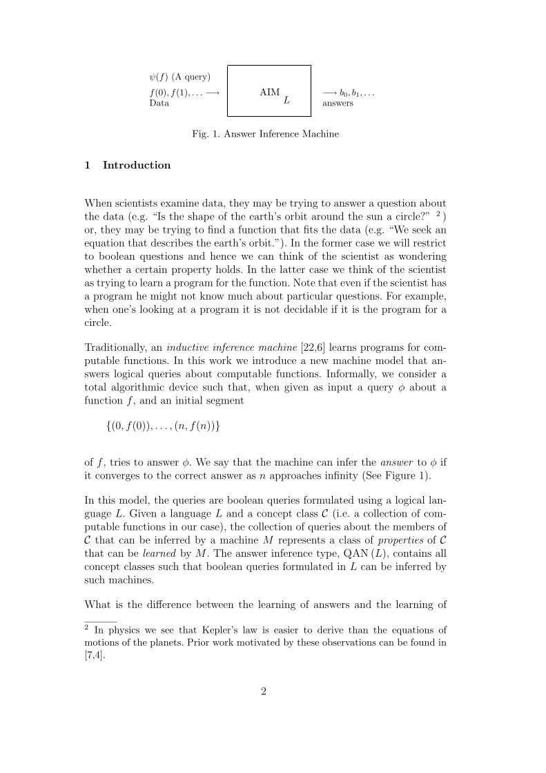
AIML
ψ(f) (A query)
f(0), f(1), . . . −→Data
−→ b0, b1, . . .answers
Fig. 1. Answer Inference Machine
1 Introduction
When scientists examine data, they may be trying to answer a question aboutthe data (e.g. “Is the shape of the earth’s orbit around the sun a circle?” 2 )or, they may be trying to find a function that fits the data (e.g. “We seek anequation that describes the earth’s orbit.”). In the former case we will restrictto boolean questions and hence we can think of the scientist as wonderingwhether a certain property holds. In the latter case we think of the scientistas trying to learn a program for the function. Note that even if the scientist hasa program he might not know much about particular questions. For example,when one’s looking at a program it is not decidable if it is the program for acircle.
Traditionally, an inductive inference machine [22,6] learns programs for com-putable functions. In this work we introduce a new machine model that an-swers logical queries about computable functions. Informally, we consider atotal algorithmic device such that, when given as input a query φ about afunction f , and an initial segment
(0, f(0)), . . . , (n, f(n))
of f , tries to answer φ. We say that the machine can infer the answer to φ ifit converges to the correct answer as n approaches infinity (See Figure 1).
In this model, the queries are boolean queries formulated using a logical lan-guage L. Given a language L and a concept class C (i.e. a collection of com-putable functions in our case), the collection of queries about the members ofC that can be inferred by a machine M represents a class of properties of Cthat can be learned by M . The answer inference type, QAN (L), contains allconcept classes such that boolean queries formulated in L can be inferred bysuch machines.
What is the difference between the learning of answers and the learning of
2 In physics we see that Kepler’s law is easier to derive than the equations ofmotions of the planets. Prior work motivated by these observations can be found in[7,4].
2
programs? In this work we show that they are strongly incomparable. We in-troduce variants of answer inference types from the machine model. They varyin their learning power. We then demonstrate the incomparability by consid-ering the extreme cases (by comparing answer inference types with standardinference types such as PEX0 and [1, n]QBCa (L)). Another theme of thispaper is to demonstrate how answer inference types can be used as a tech-nical tool in the study of query inference [19]. By examining the complexityof queries made by query inference machines, we show that separation resultsfor many standard inference types remains true for their query counterparts.This settles a number of conjectures in query inference [19,17].
There has been some related work on this problem. Smith and Wiehagen [33]introduced a model of classification, called the classification machine. Givenn collections of computable functions S1, S2, . . . , Sn, a classification machineM tries to classify the function f in the limit by converging to some i suchthat f ∈ Si. Note that a classification machine may be able to answer a singlequestion in the limit but not all the questions in a given language. In theirmodel, the Si’s are not required to be pairwise disjoint. Ben-David [5], Gasarch,Pleszkoch, Stephan and Velauthapillai [21], and Kelly [24] had studied themodel where there is no limits on computational power. Kelly’s work [24]includes the case when there are limits on computational power. In [21], themodels consider all inputs that are elements of Nω, including those that arenot computable. Other works in computable classification includes [31,8]. Werefer interested readers to these papers and the references cited therein oncomputable classification and other related topics.
The arrangement of this paper is as follows. In Section 2 we define our nota-tions and the basic terms used in the study of answer inference types. We alsostate relevant definitions from Buchi automata, query languages and relatedconcepts there. In Section 3 we summarize our technical results. Structuralproperties of answer inference types are discussed from Section 4 to Section 6.In Section 7 we demonstrate that the learning of programs and the learning ofproperties are incomparable by presenting two extreme cases. In Section 8 wefurther apply our techniques to prove a lifting lemma. It sharpens the compar-ison result in the previous section. It also enables us to obtain results aboutquery inference [19] immediately from their passive versions. Concluding re-marks and open problems will be stated in the last section.
2 Notations and Definitions
3
2.1 Standard Notations
We assume familiarity with standard definitions and notations from logic [16],computability theory [34,32] and inductive inference [3,9,23]. Throughout thiswork N = 0, 1, . . . denotes the set of all natural numbers. Given a finite setA, |A| denotes the cardinality of A and Aω denotes the set of infinite stringsof length ω formed by the elements in A. f [n] denotes the initial segment(0, f(0)), . . . , (n, f(n)) of the graph of f . We use the symbol DEC to denotethe collection of all computable functions from N to N. DEC0,1 denotes theset of all decidable subsets of N. We often think of subsets of N as 0, 1-valued functions and interpret DEC0,1 as a subset of DEC. Subsets of DECand DEC0,1 are referred as concept classes and EX, [1, n]BC and etc. (resp.QEX (L), [1, n]QBC (L) . . .) are referred as passive (resp. query) inferencetypes.
2.2 Query Languages
A First Order Query Language ([19,17]) L consists of the usual logical symbols(including equality), symbols for number variables, symbols for every elementof N, a special function symbol F denoting a function we wish to learn, andsymbols for additional functions and relations on N. We will assume thatthese additional functions and relations are computable. L may be denotedby the symbols for the additional functions and relations (e.g. [+, <] denotesthe language with additional symbols for + and <; [∅] denotes the languagewith no additional symbols). A well-formed formula over L is defined in theusual manner. Throughout this work, L denotes a reasonable query language.That is, all the symbols in L represent computable operations. The languagethat omits the symbol F from L is called the base language of L. We saythat the base language is decidable if the truth of any sentences in the baselanguage is decidable. The truth value of any sentence is either 1 (TRUE)or 0 (FALSE). We define query about functions. They are boolean questionsthat can be formulated in L. The analogous notions for sets can be definedsimilarly.
Definition 2.1 A query φ about f is a closed well-formed formula in L withthe function symbol F . φ(f) denotes both the question (when F is interpretedas f) and the correct answer (∈ 0, 1) of the question.
Note that ‘∀φ ∈ L’ denotes the phrase “for every query formulated in thelanguage L”. Some examples of queries in various languages are listed in Fig-ure 2.
4

L Example
[∅] query: (∀y)(∃x)[F(x) = y]
interpretation: ‘Is the function surjective?’
[<] query :(∃x)(∀y)[(x < y)→ F(x) = 0]
interpretation: ‘Does the function has finite support?’
[+, <] query: (∃x)(∃p)(∀y)[(x < y) ∧ (p > 0)→ F(y) = F(y + p)]
interpretation: ‘Is the function eventually periodic?’
Fig. 2. Examples of queries in different languages
Consider the query language [+,×]. It is known that questions to the HALT-ING PROBLEM can be asked in this language [14,25,13,26]. Hence the set ofall computable functions can be inferred with [+,×]. These questions are notabout the function F and not really in the spirit of our inquiry. Unless oth-erwise stated, our primary concern will be query languages with a decidablebase language.
We also use the following predicate and function symbols in some query lan-guages.
Notation 2.2 Let b ≥ 2. The following symbols will be used in some of ourquery languages:
a) Succ denotes the successor function Succ(x)=x+ 1.b) POWb is the unary predicate that determines if a number is in the setbn : n ∈ N.
c) POLYb is the unary predicate that determines if a number is in the setnb : n ∈ N.
d) FAC is the unary predicate that determines if a number is in the set n! :n ∈ N.
The query language [Succ, <]2 will be used frequently in this paper. Apartfrom the extra symbols Succ and <, we allow the use of set variables and theirquantifications (the superscript 2 is used to denote this fact). We adopt thefollowing conventions. Small (resp. Large) letters are used for number (resp.set) variables, which range over N (resp. subsets of N). Specific features of thisquery language will be addressed in later sections.
Definition 2.3 The Second Order Query language [Succ, <]2 is defined asfollows.
a) Terms: a term is either a numeric variable, a numerical constant k (inter-
5

preted as the natural number k), or is of the form g(t), where t is a termand g is either the symbol Succ or F . Note that a term does not use setvariables.
b) Atomic formulas: any atomic formula is of the form (t ∈ X), (s = t), (s < t)where s and t are terms and X is a set variable.
c) Well-formed formulas: well-formed formulas in the query language [Succ, <]2
are defined inductively as follows:(1) Any atomic formula is a well-formed formula.(2) If ψ and θ are well-formed formulas, then (ψ) ∨ (θ), (ψ) ∧ (θ), (ψ)→ (θ),
(ψ)↔ (θ) and ¬(θ) are well-formed formulas.(3) If x is a numeric variable,X is a set variable and θ is a well-formed formula,
then (∃x)[θ(x)], (∀x)[θ(x)], (∃X)[θ(X)], and (∀X)[θ(X)] are well-formedformulas.
(4) Nothing else is a well-formed formula.d) Queries: queries are the closed well-formed formulas with the function sym-
bol F .
2.3 Answer Inference Types
Definition 2.4
a) An answer inference machine M (abbrev. AIM) is a total Turing machinesuch that on each input φ ∈ L and each initial segment f [n] (n ≥ 0) of f ,output a guess of the truth value of φ(f), which is denoted by M(φ, f [n]) ∈0, 1. The limit limn→∞M(φ, f [n]) is denoted by M(φ, f) whenever itexists.
b) M infers the correct answer of φ(f) if M(φ, f) = φ(f).c) Given C ⊆ DEC. We write
C ⊆ QAN (L)(M) if (∀φ ∈ L)(∀f ∈ C)[M(φ, f) = φ(f)] and
QAN (L) = C ⊆ DEC : (∃M)[C ⊆ QAN (L)(M)].
d) The inference types QiANj (L) (i, j ≥ 0, i 6= 0) denotes the case when thequeries considered have at most i − 1 alternations of quantifiers and theanswer inference machines can make at most j mindchanges. We omit theappropriate subscripts when no restrictions are made in the correspondingcase. We will, in text, refer to this as i = ∗ or j = ∗. For example wemay say “when i ∈ N ∪ ∗ then . . .”. We call QiANj (L) trivial whenDEC ∈ QiANj (L).
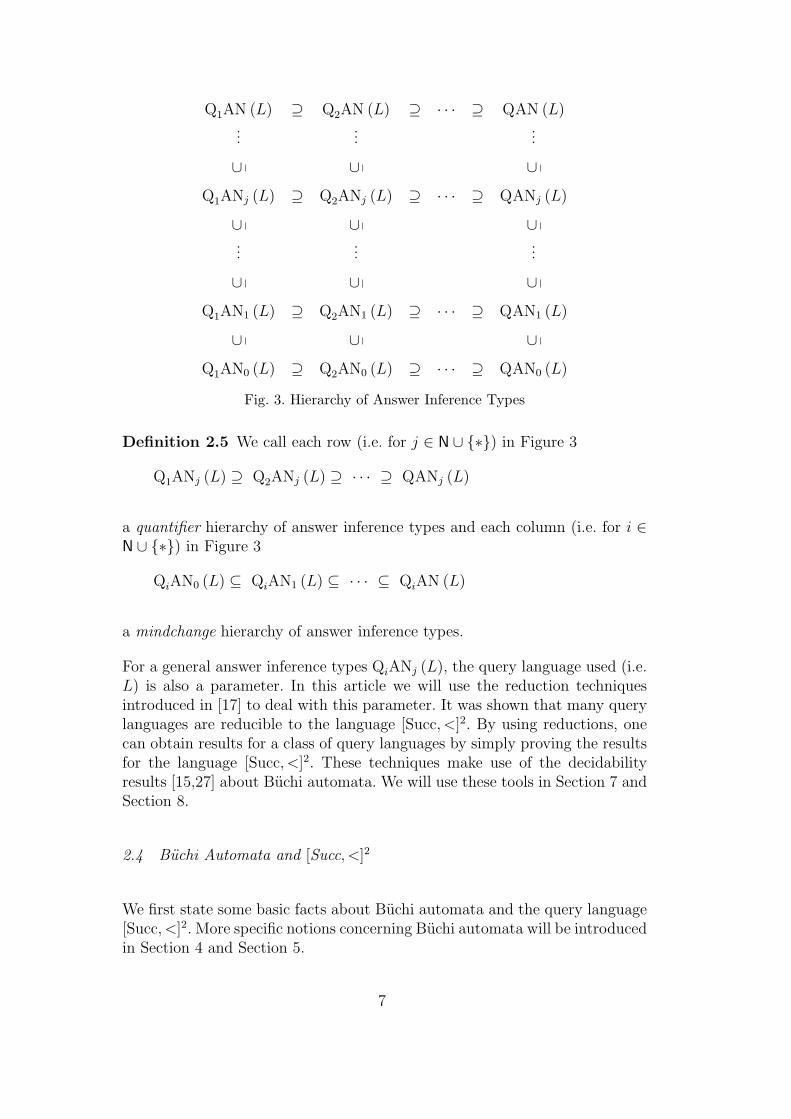
The inclusion relations described in Figure 3 follows immediately from Defi-nition 2.4.
6
Q1AN (L) ⊇ Q2AN (L) ⊇ · · · ⊇ QAN (L)...
......
∪ ∪ ∪
Q1ANj (L) ⊇ Q2ANj (L) ⊇ · · · ⊇ QANj (L)
∪ ∪ ∪...
......
∪ ∪ ∪
Q1AN1 (L) ⊇ Q2AN1 (L) ⊇ · · · ⊇ QAN1 (L)
∪ ∪ ∪
Q1AN0 (L) ⊇ Q2AN0 (L) ⊇ · · · ⊇ QAN0 (L)
Fig. 3. Hierarchy of Answer Inference Types
Definition 2.5 We call each row (i.e. for j ∈ N ∪ ∗) in Figure 3
Q1ANj (L) ⊇ Q2ANj (L) ⊇ · · · ⊇ QANj (L)
a quantifier hierarchy of answer inference types and each column (i.e. for i ∈N ∪ ∗) in Figure 3
QiAN0 (L) ⊆ QiAN1 (L) ⊆ · · · ⊆ QiAN (L)
a mindchange hierarchy of answer inference types.
For a general answer inference types QiANj (L), the query language used (i.e.L) is also a parameter. In this article we will use the reduction techniquesintroduced in [17] to deal with this parameter. It was shown that many querylanguages are reducible to the language [Succ, <]2. By using reductions, onecan obtain results for a class of query languages by simply proving the resultsfor the language [Succ, <]2. These techniques make use of the decidabilityresults [15,27] about Buchi automata. We will use these tools in Section 7 andSection 8.
2.4 Buchi Automata and [Succ, <]2
We first state some basic facts about Buchi automata and the query language[Succ, <]2. More specific notions concerning Buchi automata will be introducedin Section 4 and Section 5.
7
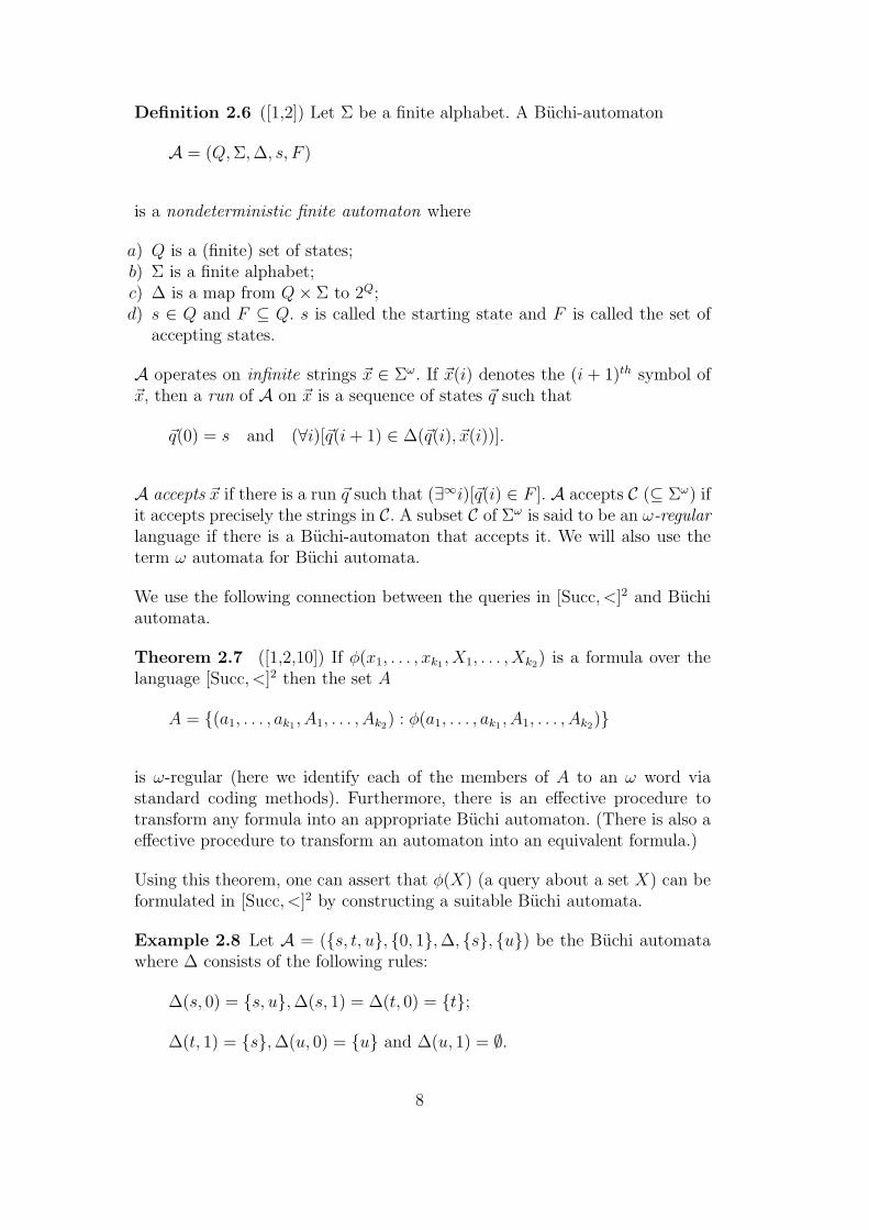
Definition 2.6 ([1,2]) Let Σ be a finite alphabet. A Buchi-automaton
A = (Q,Σ,∆, s, F )
is a nondeterministic finite automaton where
a) Q is a (finite) set of states;b) Σ is a finite alphabet;c) ∆ is a map from Q× Σ to 2Q;d) s ∈ Q and F ⊆ Q. s is called the starting state and F is called the set of
accepting states.
A operates on infinite strings ~x ∈ Σω. If ~x(i) denotes the (i + 1)th symbol of~x, then a run of A on ~x is a sequence of states ~q such that
~q(0) = s and (∀i)[~q(i+ 1) ∈ ∆(~q(i), ~x(i))].
A accepts ~x if there is a run ~q such that (∃∞i)[~q(i) ∈ F ]. A accepts C (⊆ Σω) ifit accepts precisely the strings in C. A subset C of Σω is said to be an ω-regularlanguage if there is a Buchi-automaton that accepts it. We will also use theterm ω automata for Buchi automata.
We use the following connection between the queries in [Succ, <]2 and Buchiautomata.
Theorem 2.7 ([1,2,10]) If φ(x1, . . . , xk1 , X1, . . . , Xk2) is a formula over thelanguage [Succ, <]2 then the set A
A = (a1, . . . , ak1 , A1, . . . , Ak2) : φ(a1, . . . , ak1 , A1, . . . , Ak2)
is ω-regular (here we identify each of the members of A to an ω word viastandard coding methods). Furthermore, there is an effective procedure totransform any formula into an appropriate Buchi automaton. (There is also aeffective procedure to transform an automaton into an equivalent formula.)
Using this theorem, one can assert that φ(X) (a query about a set X) can beformulated in [Succ, <]2 by constructing a suitable Buchi automata.
Example 2.8 Let A = (s, t, u, 0, 1,∆, s, u) be the Buchi automatawhere ∆ consists of the following rules:
∆(s, 0) = s, u,∆(s, 1) = ∆(t, 0) = t;
∆(t, 1) = s,∆(u, 0) = u and ∆(u, 1) = ∅.
8
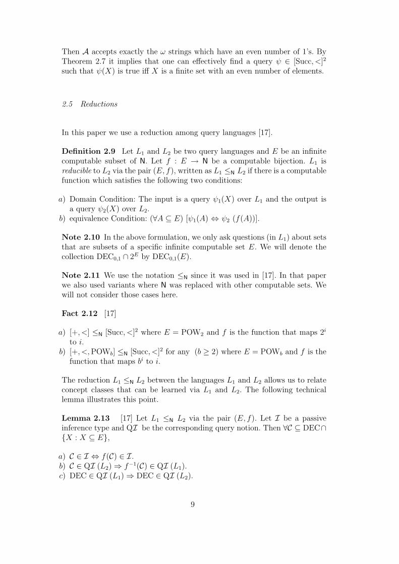
Then A accepts exactly the ω strings which have an even number of 1’s. ByTheorem 2.7 it implies that one can effectively find a query ψ ∈ [Succ, <]2
such that ψ(X) is true iff X is a finite set with an even number of elements.
2.5 Reductions
In this paper we use a reduction among query languages [17].
Definition 2.9 Let L1 and L2 be two query languages and E be an infinitecomputable subset of N. Let f : E → N be a computable bijection. L1 isreducible to L2 via the pair (E, f), written as L1 ≤N L2 if there is a computablefunction which satisfies the following two conditions:
a) Domain Condition: The input is a query ψ1(X) over L1 and the output isa query ψ2(X) over L2.
b) equivalence Condition: (∀A ⊆ E) [ψ1(A) ⇔ ψ2 (f(A))].
Note 2.10 In the above formulation, we only ask questions (in L1) about setsthat are subsets of a specific infinite computable set E. We will denote thecollection DEC0,1 ∩ 2E by DEC0,1(E).
Note 2.11 We use the notation ≤N since it was used in [17]. In that paperwe also used variants where N was replaced with other computable sets. Wewill not consider those cases here.
Fact 2.12 [17]
a) [+, <] ≤N [Succ, <]2 where E = POW2 and f is the function that maps 2i
to i.b) [+, <,POWb] ≤N [Succ, <]2 for any (b ≥ 2) where E = POWb and f is the
function that maps bi to i.
The reduction L1 ≤N L2 between the languages L1 and L2 allows us to relateconcept classes that can be learned via L1 and L2. The following technicallemma illustrates this point.
Lemma 2.13 [17] Let L1 ≤N L2 via the pair (E, f). Let I be a passiveinference type and QI be the corresponding query notion. Then ∀C ⊆ DEC∩X : X ⊆ E,
a) C ∈ I ⇔ f(C) ∈ I.b) C ∈ QI (L2)⇒ f−1(C) ∈ QI (L1).c) DEC ∈ QI (L1)⇒ DEC ∈ QI (L2).
9
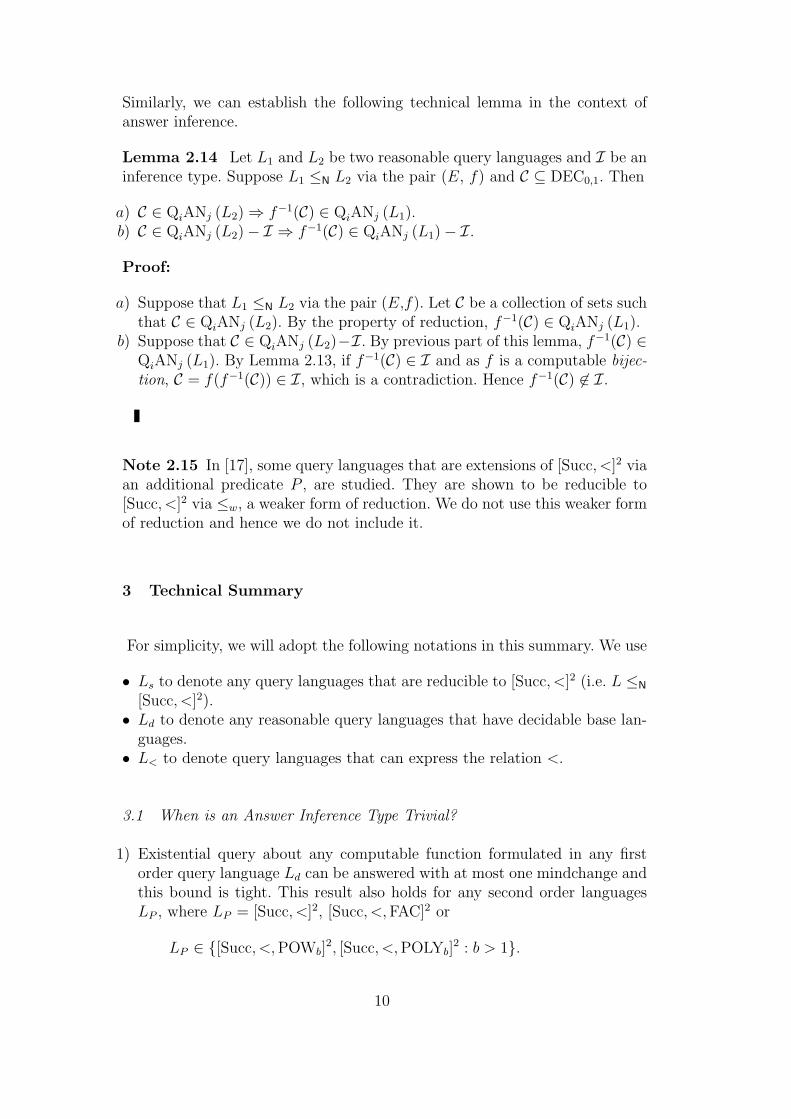
Similarly, we can establish the following technical lemma in the context ofanswer inference.
Lemma 2.14 Let L1 and L2 be two reasonable query languages and I be aninference type. Suppose L1 ≤N L2 via the pair (E, f) and C ⊆ DEC0,1. Then
a) C ∈ QiANj (L2)⇒ f−1(C) ∈ QiANj (L1).b) C ∈ QiANj (L2)− I ⇒ f−1(C) ∈ QiANj (L1)− I.
Proof:
a) Suppose that L1 ≤N L2 via the pair (E,f). Let C be a collection of sets suchthat C ∈ QiANj (L2). By the property of reduction, f−1(C) ∈ QiANj (L1).
b) Suppose that C ∈ QiANj (L2)−I. By previous part of this lemma, f−1(C) ∈QiANj (L1). By Lemma 2.13, if f−1(C) ∈ I and as f is a computable bijec-tion, C = f(f−1(C)) ∈ I, which is a contradiction. Hence f−1(C) 6∈ I.
Note 2.15 In [17], some query languages that are extensions of [Succ, <]2 viaan additional predicate P , are studied. They are shown to be reducible to[Succ, <]2 via ≤w, a weaker form of reduction. We do not use this weaker formof reduction and hence we do not include it.
3 Technical Summary
For simplicity, we will adopt the following notations in this summary. We use
• Ls to denote any query languages that are reducible to [Succ, <]2 (i.e. L ≤N
[Succ, <]2).• Ld to denote any reasonable query languages that have decidable base lan-
guages.• L< to denote query languages that can express the relation <.
3.1 When is an Answer Inference Type Trivial?
1) Existential query about any computable function formulated in any firstorder query language Ld can be answered with at most one mindchange andthis bound is tight. This result also holds for any second order languagesLP , where LP = [Succ, <]2, [Succ, <,FAC]2 or
LP ∈ [Succ, <,POWb]2, [Succ, <,POLYb]
2 : b > 1.
10
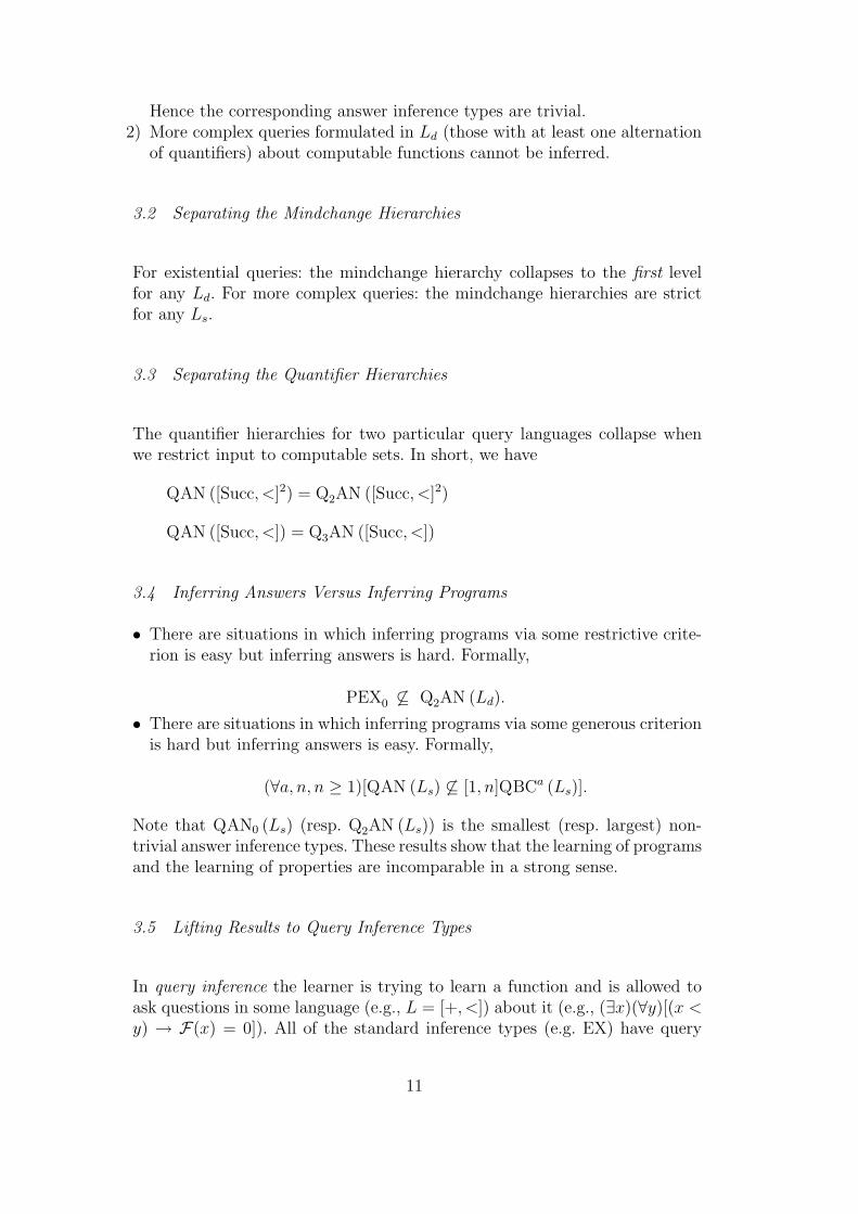
Hence the corresponding answer inference types are trivial.2) More complex queries formulated in Ld (those with at least one alternation
of quantifiers) about computable functions cannot be inferred.
3.2 Separating the Mindchange Hierarchies
For existential queries: the mindchange hierarchy collapses to the first levelfor any Ld. For more complex queries: the mindchange hierarchies are strictfor any Ls.
3.3 Separating the Quantifier Hierarchies
The quantifier hierarchies for two particular query languages collapse whenwe restrict input to computable sets. In short, we have
QAN ([Succ, <]2) = Q2AN ([Succ, <]2)
QAN ([Succ, <]) = Q3AN ([Succ, <])
3.4 Inferring Answers Versus Inferring Programs
• There are situations in which inferring programs via some restrictive crite-rion is easy but inferring answers is hard. Formally,
PEX0 6⊆ Q2AN (Ld).
• There are situations in which inferring programs via some generous criterionis hard but inferring answers is easy. Formally,
(∀a, n, n ≥ 1)[QAN (Ls) 6⊆ [1, n]QBCa (Ls)].
Note that QAN0 (Ls) (resp. Q2AN (Ls)) is the smallest (resp. largest) non-trivial answer inference types. These results show that the learning of programsand the learning of properties are incomparable in a strong sense.
3.5 Lifting Results to Query Inference Types
In query inference the learner is trying to learn a function and is allowed toask questions in some language (e.g., L = [+, <]) about it (e.g., (∃x)(∀y)[(x <y) → F(x) = 0]). All of the standard inference types (e.g. EX) have query
11
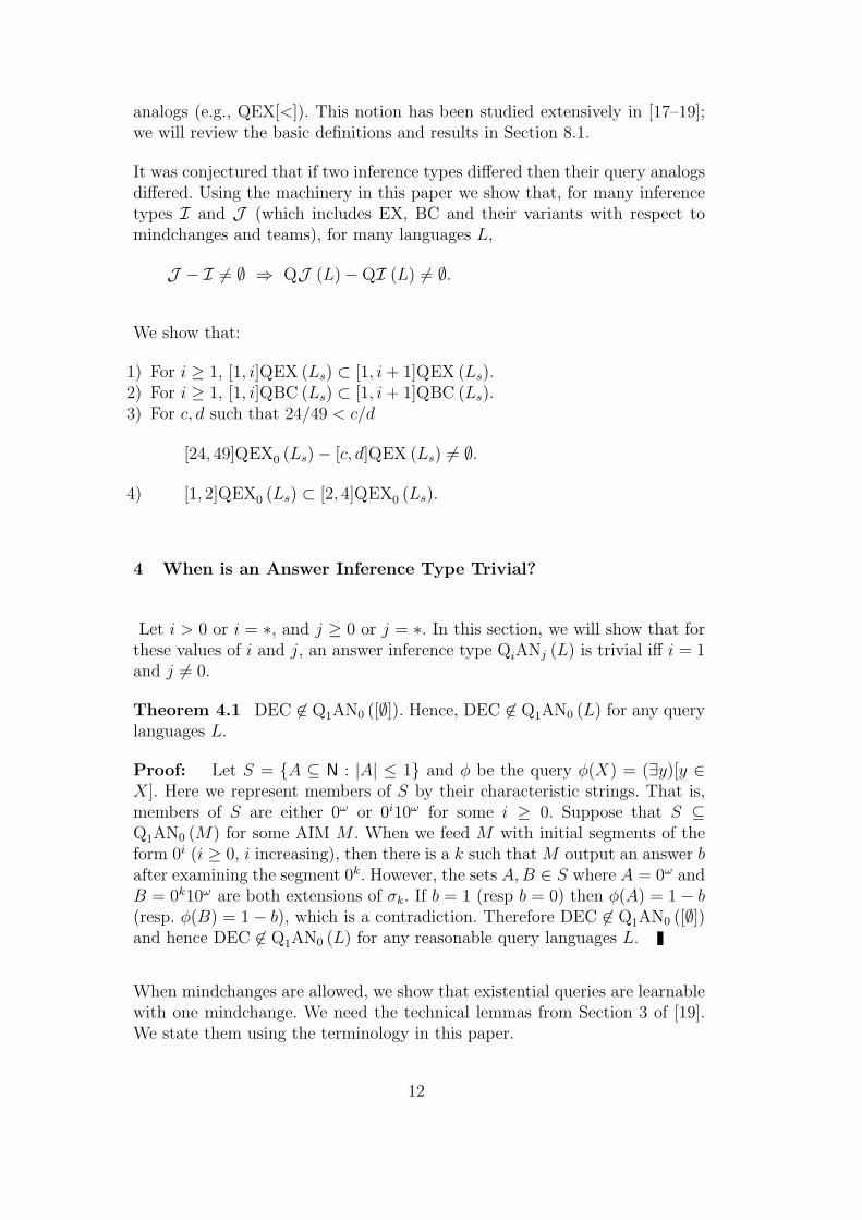
analogs (e.g., QEX[<]). This notion has been studied extensively in [17–19];we will review the basic definitions and results in Section 8.1.
It was conjectured that if two inference types differed then their query analogsdiffered. Using the machinery in this paper we show that, for many inferencetypes I and J (which includes EX, BC and their variants with respect tomindchanges and teams), for many languages L,
J − I 6= ∅ ⇒ QJ (L)−QI (L) 6= ∅.
We show that:
1) For i ≥ 1, [1, i]QEX (Ls) ⊂ [1, i+ 1]QEX (Ls).2) For i ≥ 1, [1, i]QBC (Ls) ⊂ [1, i+ 1]QBC (Ls).3) For c, d such that 24/49 < c/d
[24, 49]QEX0 (Ls)− [c, d]QEX (Ls) 6= ∅.
4) [1, 2]QEX0 (Ls) ⊂ [2, 4]QEX0 (Ls).
4 When is an Answer Inference Type Trivial?
Let i > 0 or i = ∗, and j ≥ 0 or j = ∗. In this section, we will show that forthese values of i and j, an answer inference type QiANj (L) is trivial iff i = 1and j 6= 0.
Theorem 4.1 DEC 6∈ Q1AN0 ([∅]). Hence, DEC 6∈ Q1AN0 (L) for any querylanguages L.
Proof: Let S = A ⊆ N : |A| ≤ 1 and φ be the query φ(X) = (∃y)[y ∈X]. Here we represent members of S by their characteristic strings. That is,members of S are either 0ω or 0i10ω for some i ≥ 0. Suppose that S ⊆Q1AN0 (M) for some AIM M . When we feed M with initial segments of theform 0i (i ≥ 0, i increasing), then there is a k such that M output an answer bafter examining the segment 0k. However, the sets A,B ∈ S where A = 0ω andB = 0k10ω are both extensions of σk. If b = 1 (resp b = 0) then φ(A) = 1− b(resp. φ(B) = 1− b), which is a contradiction. Therefore DEC 6∈ Q1AN0 ([∅])and hence DEC 6∈ Q1AN0 (L) for any reasonable query languages L.
When mindchanges are allowed, we show that existential queries are learnablewith one mindchange. We need the technical lemmas from Section 3 of [19].We state them using the terminology in this paper.
12
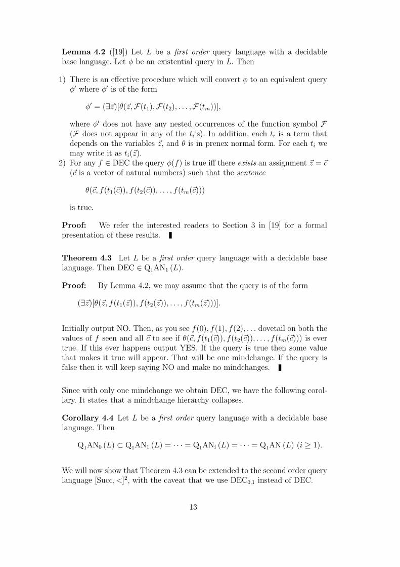
Lemma 4.2 ([19]) Let L be a first order query language with a decidablebase language. Let φ be an existential query in L. Then
1) There is an effective procedure which will convert φ to an equivalent queryφ′ where φ′ is of the form
φ′ = (∃~z)[θ(~z,F(t1),F(t2), . . . ,F(tm))],
where φ′ does not have any nested occurrences of the function symbol F(F does not appear in any of the ti’s). In addition, each ti is a term thatdepends on the variables ~z, and θ is in prenex normal form. For each ti wemay write it as ti(~z).
2) For any f ∈ DEC the query φ(f) is true iff there exists an assignment ~z = ~c(~c is a vector of natural numbers) such that the sentence
θ(~c, f(t1(~c)), f(t2(~c)), . . . , f(tm(~c)))
is true.
Proof: We refer the interested readers to Section 3 in [19] for a formalpresentation of these results.
Theorem 4.3 Let L be a first order query language with a decidable baselanguage. Then DEC ∈ Q1AN1 (L).
Proof: By Lemma 4.2, we may assume that the query is of the form
(∃~z)[θ(~z, f(t1(~z)), f(t2(~z)), . . . , f(tm(~z)))].
Initially output NO. Then, as you see f(0), f(1), f(2), . . . dovetail on both thevalues of f seen and all ~c to see if θ(~c, f(t1(~c)), f(t2(~c)), . . . , f(tm(~c))) is evertrue. If this ever happens output YES. If the query is true then some valuethat makes it true will appear. That will be one mindchange. If the query isfalse then it will keep saying NO and make no mindchanges.
Since with only one mindchange we obtain DEC, we have the following corol-lary. It states that a mindchange hierarchy collapses.
Corollary 4.4 Let L be a first order query language with a decidable baselanguage. Then
Q1AN0 (L) ⊂ Q1AN1 (L) = · · · = Q1ANi (L) = · · · = Q1AN (L) (i ≥ 1).
We will now show that Theorem 4.3 can be extended to the second order querylanguage [Succ, <]2, with the caveat that we use DEC0,1 instead of DEC.
13
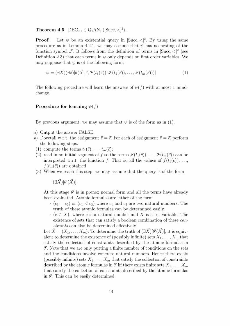
Theorem 4.5 DEC0,1 ∈ Q1AN1 ([Succ, <]2).
Proof: Let ψ be an existential query in [Succ, <]2. By using the sameprocedure as in Lemma 4.2.1, we may assume that ψ has no nesting of thefunction symbol F . It follows from the definition of terms in [Succ, <]2 (seeDefinition 2.3) that each terms in ψ only depends on first order variables. Wemay suppose that ψ is of the following form:
ψ = (∃ ~X)(∃~z)[θ( ~X, ~z,F(t1(~z)),F(t2(~z)), . . . ,F(tm(~z)))] (1)
The following procedure will learn the answers of ψ(f) with at most 1 mind-change.
Procedure for learning ψ(f)
By previous argument, we may assume that ψ is of the form as in (1).
a) Output the answer FALSE.b) Dovetail w.r.t. the assignment ~z = ~c. For each of assignment ~z = ~c, perform
the following steps:(1) compute the terms t1(~c), . . . , tm(~c);(2) read in an initial segment of f so the terms F(t1(~c)), . . . ,F(tm(~c)) can be
interpreted w.r.t. the function f . That is, all the values of f(t1(~c)), . . .,f(tm(~c)) are obtained.
(3) When we reach this step, we may assume that the query is of the form
(∃ ~X)[θ′( ~X)].
At this stage θ′ is in prenex normal form and all the terms have alreadybeen evaluated. Atomic formulas are either of the form· (c1 = c2) or (c1 < c2) where c1 and c2 are two natural numbers. The
truth of these atomic formulas can be determined easily.· (c ∈ X), where c is a natural number and X is a set variable. The
existence of sets that can satisfy a boolean combination of these con-straints can also be determined effectively.
Let ~X = (X1, . . . , Xm). To determine the truth of (∃ ~X)[θ′( ~X)], it is equiv-alent to determine the existence of (possibly infinite) sets X1, . . . , Xm thatsatisfy the collection of constraints described by the atomic formulas inθ′. Note that we are only putting a finite number of conditions on the setsand the conditions involve concrete natural numbers. Hence there exists(possibly infinite) sets X1, . . . , Xm that satisfy the collection of constraintsdescribed by the atomic formulas in θ′ iff there exists finite setsX1, . . . , Xm
that satisfy the collection of constraints described by the atomic formulasin θ′. This can be easily determined.
14
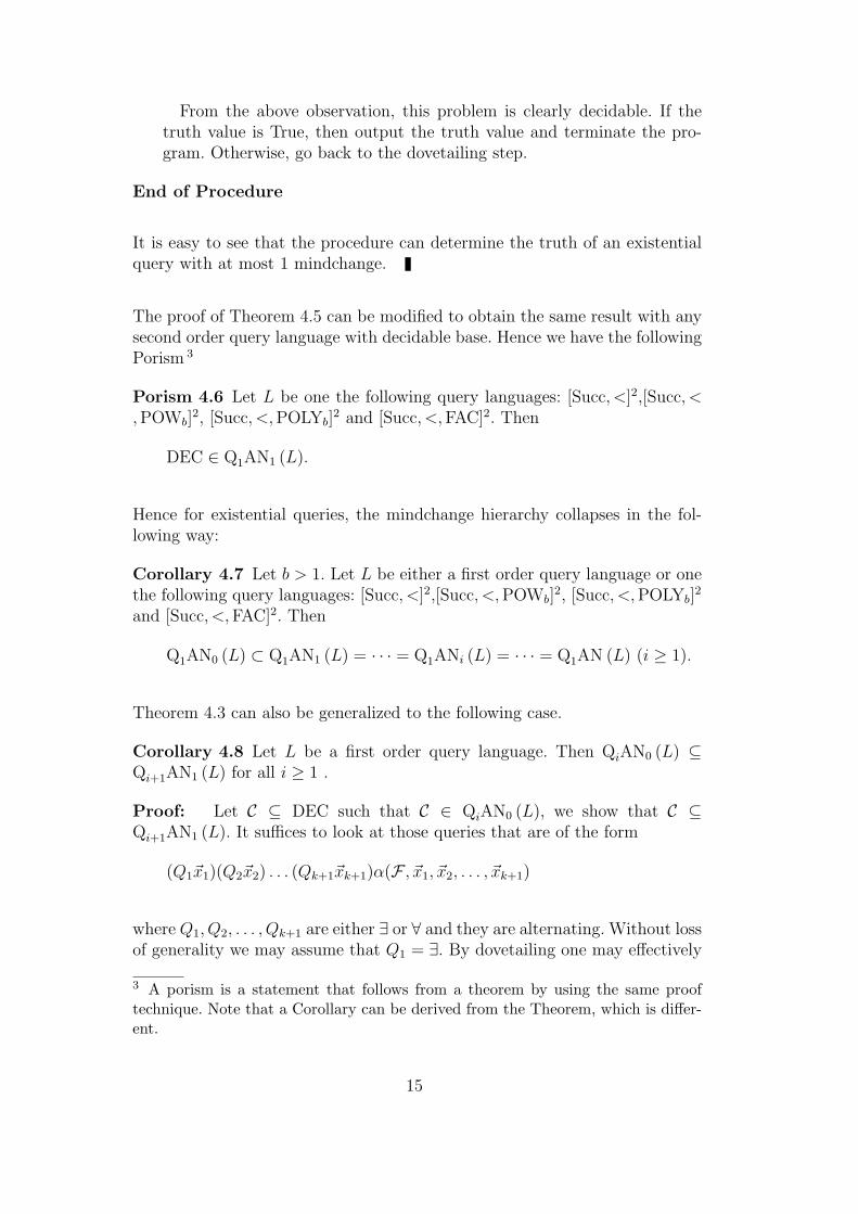
From the above observation, this problem is clearly decidable. If thetruth value is True, then output the truth value and terminate the pro-gram. Otherwise, go back to the dovetailing step.
End of Procedure
It is easy to see that the procedure can determine the truth of an existentialquery with at most 1 mindchange.
The proof of Theorem 4.5 can be modified to obtain the same result with anysecond order query language with decidable base. Hence we have the followingPorism 3
Porism 4.6 Let L be one the following query languages: [Succ, <]2,[Succ, <,POWb]
2, [Succ, <,POLYb]2 and [Succ, <,FAC]2. Then
DEC ∈ Q1AN1 (L).
Hence for existential queries, the mindchange hierarchy collapses in the fol-lowing way:
Corollary 4.7 Let b > 1. Let L be either a first order query language or onethe following query languages: [Succ, <]2,[Succ, <,POWb]
2, [Succ, <,POLYb]2
and [Succ, <,FAC]2. Then
Q1AN0 (L) ⊂ Q1AN1 (L) = · · · = Q1ANi (L) = · · · = Q1AN (L) (i ≥ 1).
Theorem 4.3 can also be generalized to the following case.
Corollary 4.8 Let L be a first order query language. Then QiAN0 (L) ⊆Qi+1AN1 (L) for all i ≥ 1 .
Proof: Let C ⊆ DEC such that C ∈ QiAN0 (L), we show that C ⊆Qi+1AN1 (L). It suffices to look at those queries that are of the form
(Q1~x1)(Q2~x2) . . . (Qk+1~xk+1)α(F , ~x1, ~x2, . . . , ~xk+1)
where Q1, Q2, . . . , Qk+1 are either ∃ or ∀ and they are alternating. Without lossof generality we may assume that Q1 = ∃. By dovetailing one may effectively
3 A porism is a statement that follows from a theorem by using the same prooftechnique. Note that a Corollary can be derived from the Theorem, which is differ-ent.
15
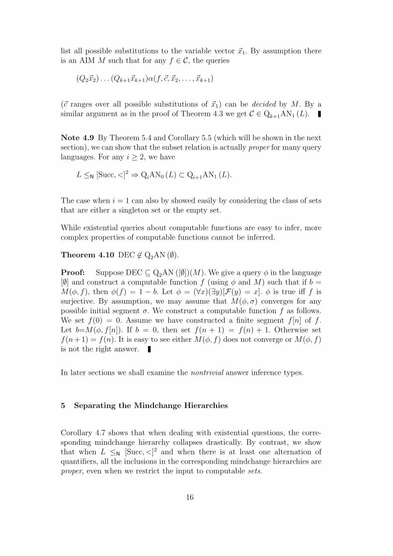
list all possible substitutions to the variable vector ~x1. By assumption thereis an AIM M such that for any f ∈ C, the queries
(Q2~x2) . . . (Qk+1~xk+1)α(f,~c, ~x2, . . . , ~xk+1)
(~c ranges over all possible substitutions of ~x1) can be decided by M . By asimilar argument as in the proof of Theorem 4.3 we get C ∈ Qk+1AN1 (L).
Note 4.9 By Theorem 5.4 and Corollary 5.5 (which will be shown in the nextsection), we can show that the subset relation is actually proper for many querylanguages. For any i ≥ 2, we have
L ≤N [Succ, <]2 ⇒ QiAN0 (L) ⊂ Qi+1AN1 (L).
The case when i = 1 can also by showed easily by considering the class of setsthat are either a singleton set or the empty set.
While existential queries about computable functions are easy to infer, morecomplex properties of computable functions cannot be inferred.
Theorem 4.10 DEC 6∈ Q2AN (∅).
Proof: Suppose DEC ⊆ Q2AN ([∅])(M). We give a query φ in the language[∅] and construct a computable function f (using φ and M) such that if b =M(φ, f), then φ(f) = 1 − b. Let φ = (∀x)(∃y)[F(y) = x]. φ is true iff f issurjective. By assumption, we may assume that M(φ, σ) converges for anypossible initial segment σ. We construct a computable function f as follows.We set f(0) = 0. Assume we have constructed a finite segment f [n] of f .Let b=M(φ, f [n]). If b = 0, then set f(n + 1) = f(n) + 1. Otherwise setf(n+1) = f(n). It is easy to see either M(φ, f) does not converge or M(φ, f)is not the right answer.
In later sections we shall examine the nontrivial answer inference types.
5 Separating the Mindchange Hierarchies
Corollary 4.7 shows that when dealing with existential questions, the corre-sponding mindchange hierarchy collapses drastically. By contrast, we showthat when L ≤N [Succ, <]2 and when there is at least one alternation ofquantifiers, all the inclusions in the corresponding mindchange hierarchies areproper, even when we restrict the input to computable sets.
16
Definition 5.1 Let A ⊆ N and L be a reasonable query language. A is saidto be definable by a query φ in L if there is a query φ(X) ∈ L such that φ(X)is true if and only if X = A.
Intuitively, these sets are those that can be described precisely by a query.For example, any finite and co-finite sets are definable via a query in anyreasonable query language. The set of all even numbers is also definable in thelanguage [Succ] via the query
φ(X) = (0 ∈ X) ∧ (1 /∈ X) ∧ (∀y)[y ∈ X ⇔ Succ(Succ(y)) ∈ X]
We will now show that the mindchange hierarchies for non-existential queriesare proper. To simplify our presentation, we introduce the following definitions.
Definition 5.2
a) Let A,B ⊆ N. B is said to be a k-variant of A if the symmetric differenceof the sets A and B (denoted by A∆B) has precisely k elements. Note thatthe size of A∆B can be written as |A−B|+ |B − A|.
b) For any A ∈ DEC0,1, we define the k-ball of A to be the set
Sk(A) = B ∈ DEC0,1 : |A∆B| ≤ k.
Lemma 5.3
a) Let A be a set that is definable by a query φA in the language L. Then forany j,m ∈ N, the question
‘Is X a j-variant of A, where j is an odd number and j ≤ m ?’can be expressed as a query in L of the form
(∃Y )(∃x1, . . . , xk)(∀y)[E1 ∧ E2 ∧ E3].
We will denote this query by ηodd(A,X,m).b) For any set A that is definable by a query φA in the language [Succ, <]2 and
for any k ≥ 1,
Sk(A) ∈ QANk ([Succ, <]2).
Proof:
a) First note that
u ∈ X∆Y iff [[(u ∈ X) ∧ (u /∈ Y )] ∨ [(u /∈ X) ∧ (u ∈ Y )]]
and that A is definable in L via φA. The question‘Is X a j-variant of A ?’
17
can be represented by the following query φj,A(X) in L:
φj,A(X) = (∃Y )(∃x1)(∃x2) · · · (∃xj)(∀y)(E1 ∧ E2 ∧ E3)
where E1, E2 and E3 are the expressions
E1 :∧
n6=m,n,m≤j
(xn 6= xm); E2 : φA(Y ); E3 : [(y ∈ Y∆X)⇔j∨
n=1
(y = xn)]
Hence, the question
‘Is X a j-variant of A, where j is an odd number and j ≤ m ?’
can be expressed as
ηodd(A,X,m) =∨
j∈1,...,m∧j oddφj,A(X).
As each φj,A(X) is a query in L, ηodd(A,X,m) is a query in L.b) Let φ(X) ∈ [Succ, <]2 and B ∈ Sk(A), we can infer the answer to φ(B) as
follows. Initially we guess that φ(B)=φ(A). To decide the truth of φ(A),we construct a Buchi automaton Aφ for φ(X) (Keep this automaton, wewill use it later in the algorithm also.) Since A is definable by a query in[Succ, <]2, we can construct a Buchi automaton A that accepts only A.Now construct the intersection of Aφ and A and test for emptiness. As theemptiness problem of Buchi automata is decidable, the truth of the queryφ(A) can be obtained. Next, on input σ B, |σ| = n, we first find a Buchiautomaton Aσ that accepts the string σA(n)A(n+1) · · ·. We then constructthe intersection of Aφ and Aσ and test for emptiness. Note that over timethe set we are testing for intersection will change at most k times since Bis in the k-ball of A.
Theorem 5.4 Let i, k ∈ N ∪ ∗, i 6= 0, 1 and k 6= 0, ∗.
a) QANk ([Succ, <]2) 6⊆ Q2ANk−1 ([Succ, <]2).b) QiAN0 ([Succ, <]2) ⊂ QiAN1 ([Succ, <]2) ⊂ · · ·
· · · ⊂ QiANj ([Succ, <]2) ⊂ · · · ⊂ QiAN ([Succ, <]2).
Proof:
a) From part b) of Lemma 5.3 it suffices to show that for any set A that isdefinable via a query in [Succ, <]2 and for any k ≥ 1,
Sk(A) 6∈ Q2ANk−1 ([Succ, <]2).
18
Assume by way of contradiction that Sk(A) ⊆ Q2ANk−1 ([Succ, <]2)(M) forsome positive integer k. Let φ be the query ηodd(A,X, k) (from Lemma 5.3).Since A is definable via a query in [Succ, <]2, by part a) of Lemma 5.3,φ = ηodd(A,X, k) is a query in [Succ, <]2.
We shall construct a computable set B ∈ Sk(A) by diagonalizing againstM using φ as our input. B will witness the fact that M cannot infer thecorrect answer to the query φ(B). Throughout the construction, at thebeginning of any stage s we keep track of the following:
(1) Bs, the initial segment of the set B defined so far.(2) As, the initial segment of A such that dom(As)=dom(Bs).(3) ds=|x : x ∈ A∆B, x ∈ dom(As)| .(4) cs, the number of mindchanges the machine has made at the beginning of
that stage.
Construction of BLet A0 be the initial segment of A where dom(A0)=0. Let B0=A0;
a0 = 0; c0 = 0.Stage s: Compute b = M(φ,Bs) and ds. Compute as+1, which is the small-est number in A − 0, . . . , as. Let As+1 be the initial segment of A withdomain 0, . . . , as+1. Define
C = (u, 0) : as < u < as+1.
Define Bs+1 as follows.(1) If b = TRUE and ds is odd then the question “is |Bs∆A| odd” is currently
true, and is being answered correctly. We want to make it answered incor-rectly. Hence let Bs+1 = Bs ∪ C ∪ (as+1, 0). This creates another placewhere A and B differ, so they now differ in an even number of places.
(2) If b = FALSE and ds is odd then the question “is |Bs∆A| odd” is cur-rently false, but is being answered incorrectly. We want to maintain this.Bs∪C ∪(as+1, 1). This does not create another place where they differ,so they still differ in an odd number of places.
(3) If b = TRUE and ds is even then the question “is |Bs∆A| odd” is cur-rently false, but is being answered incorrectly. Hence let Bs+1 = Bs ∪C ∪(as+1, 1).
(4) If b = TRUE and ds is odd then the question “is |Bs∆A| odd” is currentlytrue, but is being answered correctly. Hence let Bs+1 = Bs∪C∪(as+1, 0).
Compute M(φ,Bs+1). If this is not equal to b then set cs+1 = cs + 1.End of Construction
Let c be the number of times thatM changes its mind during the construc-tion. By definition of M , c < k, hence there is a stage we denote t such thatat any stage t′ with t′ > t, M(φ,Bt′) = M(φ,Bt) = M(φ,B). During stage tof the construction, either there was a mindchange or there was not. If therewas no mindchange then the disagreement that we caused in this stage is
19

permanent, so 1−M(φ,Bt)=1−M(φ,B) and this answer is wrong. If therewas a mindchange then during the next stage, which we call t′, we will causea disagreement that will be permanent. Hence 1−M(φ,Bt′)=1−M(φ,B)and this answer is wrong.
Finally, we note that by choosing A =N, the query ηodd(A,X, j) (j ≥ 1)is a ∃∀ query in the language [∅]. Therefore,
Sk(N) ∈ QANk ([Succ, <]2)−QANk ([∅])
and the result follows immediately.
b) By Theorem 6.1 for any i ≥ 2 and k ≥ 1,
QANk ([Succ, <]2) ⊆ QiANk ([Succ, <]2) and
QiANk−1 ([Succ, <]2) ⊆ Q2ANk−1 ([Succ, <]2).
Suppose that QiANk ([Succ, <]2) = QiANk−1 ([Succ, <]2). Then
QANk ([Succ, <]2) ⊆ QiANk ([Succ, <]2)
= QiANk−1 ([Succ, <]2)
⊆ Q2ANk−1 ([Succ, <]2),
which implies QANk ([Succ, <]2) ⊆ Q2ANk−1 ([Succ, <]2). This contradictspart (a). Thus, for any i ≥ 2 and k ∈ N,
QiANk ([Succ, <]2) ⊂ QiANk+1 ([Succ, <]2).
Finally, suppose QiAN ([Succ, <]2) = QiANn ([Succ, <]2), for some n ∈ N.We then have
QiAN ([Succ, <]2) = QiANn ([Succ, <]2)
⊂ QiANn+1 ([Succ, <]2)
= QiAN ([Succ, <]2),
a contradiction. Therefore, for i 6= 0, 1 and k ∈ N,
QiANk ([Succ, <]2) ⊂ QiAN ([Succ, <]2)
Corollary 5.5 Let i, k ∈ N ∪ ∗, i 6= 0, 1 and k 6= 0.
a) (∀L ≤N [Succ, <]2) [ QANk (L) 6⊆ Q2ANk−1 (L) ].
20
b) For all b, QANk ([+, <,POWb]) 6⊆ Q2ANk−1 ([+, <,POWb]).c) (∀L ≤N [Succ, <]2)[ QiAN0 (L) ⊂ QiAN1 (L) ⊂ · · · ⊂ QiAN (L) ].d) For all b,
QiAN0 ([+, <,POWb]) ⊂ QiAN1 ([+, <,POWb]) ⊂ · · ·
· · · ⊂ QiANj ([+, <,POWb]) ⊂ · · · ⊂ QiAN ([+, <,POWb]).
Proof: By Theorem 5.4, and Fact 2.12.
6 Quantifier Hierarchies
It is natural to ask if the quantifier hierarchies are also strict. In this subsectionwe will give examples of quantifier hierarchies that collapse to low levels.
First, let L be either the language [Succ, <] or [Succ, <]2. Suppose that φ(X)is a query about a set X in either one of these languages. We claim that thesequeries cannot be too complex. From Theorem 2.7 we see that to test if φ(A)is true, it is equivalent to test if the characteristic string of A is accepted by acorresponding ω automata Aφ. This automata can be constructed effectivelyfrom φ. As the acceptance condition of any ω automata is itself a formulain [Succ, <]2 which uses few alternations of quantifiers, these queries cannotbe too complex. By exploring the quantifier complexity of these acceptanceformulas, we have the following results:
Theorem 6.1 When we restrict input to sets, we have
a) Q2AN ([Succ, <]2) = · · · = QjAN ([Succ, <]2) = · · · = QAN ([Succ, <]2)b) Q3AN ([Succ, <]) = · · · = QjAN ([Succ, <]) = · · · = QAN ([Succ, <])
Proof:
a) By [29], all ω regular languages can be written as the set of solutions to atwo quantifier formula in the language in [Succ, <]2.
b) By [37], any query in [Succ, <] is equivalent to a boolean combination offormulas in [Succ, <], where each formula has at most two alternations ofquantifiers.
21
Note 6.2 The results from [37] also imply the following results in answerinference and query inference (see Section 5 for basic notions on query infer-ence).
1) When restrict input to sets, QEX ([Succ, <]2) = Q2EX [[Succ, <]]2.2) When restrict input to sets, QEX ([Succ, <]) = Q3EX ([Succ, <]).
Hence, queries in the languages [Succ, <] and [Succ, <]2 are not too expressive.For L ≤N [Succ, <]2 via the pair (E,f), one can use the same idea to show thatthe corresponding quantifier hierarchy collapses locally. That is, the quantifierhierarchy collapses when we restrict our input to computable subsets of E.
It is an open question to determine if other quantifier hierarchies collapse.
7 Inferring Answers versus Inferring Programs
Recall that for many query languages L, the largest nontrivial answer infer-ence type is Q2AN (L) and the smallest is QAN0 (L) (see Figure 3). In thissection we will use them to demonstrate that the learning of answers and thelearning of programs are incomparable in a very strong sense. Our comparisonshighlight the following two extreme cases:
First Case: There are concepts that can be learned using a very restrictiveidentification criteria. However, relatively simple properties of the functionsin this class are not learnable.
Second Case: There are concepts that cannot be learned using a very gener-ous identification criteria. However, all boolean queries about the functionsin this class are learnable for many query languages.
7.1 First Case
Consider the Popperian inference type PEX0 . The learning criteria is veryrestrictive. It does not allows mindchanges and any conjectures that the ma-chine can make must be a total computable function. We compare it with thelargest nontrivial inference type Q2AN (L). The following non-inclusion holds:
Theorem 7.1 PEX0 6⊆ Q2AN (∅).
Proof: Let P0, P1, P2, . . . an effective enumeration of the primitive recursivefunctions that (1) satisfies m-ary composition, (2) satisfies the s-m-n theorem,and (2) function E(i, x) = Pi(x) is computable. (Note that any reasonable en-
22
coding of the primitive recursive functions will have these properties.). Con-sider the concept
A = f : Pf(0) = f.
Intuitively the value f(0) is the index of a primitive recursive function that isequal to f . Clearly A ∈ PEX0 .
Assume, by way of contradiction, that PEX0 ⊆ Q2AN (L) via machine M .We can assume that M is primitive recursive by slowing it down. Let φ be thequery
(∀x)(∃y)[F(y) = x].
φ(f) is true iff f is surjective. We construct a computable function f ∈ A suchthat M(φ, f) 6= φ(f).
Construction of f
Stage 0: Let f(0) be the index of this construction for f . (We can do thisby the recursion theorem for primitive recursive functions. See Theorem 4.6of [28].) Let
f(1) = 0,
f(2) = 1,
...
f(f(0))) = f(0)− 1,
and let
f(f(0) + 1) = f(0) + 1.
Let x0 = f(0) + 1. At every state xs will be such that, at the end of stage s,f(0), . . . , f(xs) are defined.
Stage s+ 1:
Compute b = M(φ, f(0)f(1) · · · f(xs)). If b = 0 (so M(φ, f(0)f(1) · · · f(xs))thinks that f is not onto) then let f(xs + 1) = f(xs) + 1. If b = 1 (so
23
M(φ, f(0)f(1) · · · f(xs)) thinks that f is onto) then let f(xs + 1) = f(xs).
End of Construction
By Stage 0, f ∈ A. If M(φ, f) converges to 0 then f will keep outputtingnumbers in order and hence f is onto. If M(φ, f) converges to 1 then f willkeep outputting the same number and hence f is not onto. Hence if M(φ, f)converges then it is incorrect. This is a contradiction.
7.2 The Omega Operator Ω
We consider another extreme case where we will show that the smallest non-trivial inference type QAN0 (L) (L ≤N [Succ, <]2) is not contained in manystandard inference types, which include EX , BC and their team variants.Our proof uses decidability results from the theory of ω-automata and we willinclude them in this section.
In addition, we use an operator approach. We construct an operator, call theomega operator, which translates appropriate concept classes to witness thecorresponding separations. A similar approach was used in [35] in the studyof query inference degrees. The decidability results about the query language[+, <] [18] were used in that case.
Informally the omega operator Ω will map each function f into a set A withcharacteristic string that is of the following form:
A = 0k0·a01 · · · 0kn·an1 · · · (kn ≥ 1 for any n.) (2)
The functional values of f are ‘coded’ into the sequence knn≥0. By usingthe structural properties of a Buchi automaton the sequence ann≥0 can becomputed so that for any set A with characteristic string of the form (2) and forany query φ(X) ∈ [Succ, <]2, φ(A) can be answered correctly without makingany mindchanges. We state the following results about Buchi automata whichwill be used in our proofs.
Definition 7.2 ([15,17]) Let Σ be a finite alphabet and σ, τ ∈ Σ. Let P bethe infinite string
P = σp0τ0 . . . σpnτn . . . ,
where p0 ≥ 0, pi > 0 for any i ≥ 1 and for all i, τi ∈ Σ − σ. Define the
24
partial function thind,σ: Σω → Σω as:
thind,σ(P ) = σq0τ0 . . . σqnτn . . . ,
where qi’s are defined by the formula
qi =
pi if pi ≤ d,
µq [[d < q ≤ d+ d!] ∧ [q ≡ pi(mod d!)]] otherwise.(3)
Theorem 7.3 ([15]) Let Σ be a finite alphabet, σ, τ ∈ Σ. Let A be a Buchiautomaton over Σ. Suppose that A has n states. Let d ≥ 2n22n
. If
X = σp0τ0 . . . σpnτn . . .
where τi ∈ Σ−σ for all i. Then X is accepted by A if and only if thind,σ(X)is accepted by A.
Note 7.4
a) Let Σ = 0, 1, σ = 0, τ = 1. Then thind,0(P ) is defined when P has theproperty of x ∈ P ⇒ x+ 1 /∈ P .
b) Given a query φ(X) ∈ [Succ, <]2, by Theorem 2.7 one can construct an ωautomata A effectively such that φ(A) is true iff the characteristic stringsof A is accepted by A. Theorem 7.3 suggests that if the number of states inA equals n, then
φ(A)⇔ φ(thind,0(A)) for any d ≥ 2n22n
.
This fact will be used in our construction of the omega operator.
Now we state the formal definition for the omega operator Ω.
Definition 7.5 Let φ0(X), φ1(X), . . . , φn(X), . . . be a computable enumer-ation of all queries about a set X in [Succ, <]2 via a fixed procedure P1.Let A0, . . . ,An, . . . be the corresponding Buchi automata obtained from thequeries via a fixed procedure P2. (Note: by Theorem 2.7, such a procedureexists). Let nj (j ∈ N) be the number of states of Aj. Define
hj = n2j2
nj ; dj = 2hj and mj = max di : 0 ≤ i ≤ j.
We identify a function f : N→ N with the string f(0) · · · f(n) · · · ∈ Nω and aset A with its characteristic string. The Omega operator Ω : Nω → 0, 1ω is
25
defined as:
Ω(f) = 0l(0,f(0))1 · · · 0l(n,f(n))1 · · · ,
where l(n, f(n)) = (f(n) + 1) ·mn! for any n.
Notation 7.6 We also use the following notations when using the operatorΩ.
a) For any C ⊆ DEC, Ω(C) = Ω(f) : f ∈ C.b) Ω denotes the transformation which takes a string f(0) . . . f(n) (identified
with f [n]) to Ω(f [n]) = 0l(0,f(0))1 . . . 0l(n,f(n))1.c) The xth position of the string Ω(f [n]) = 0l(0,f(0))1 . . . 0l(n,f(n))1 ( 0 ≤ x <∑n
i=0 l(i, f(i)) + 1) is denoted by Ω(f [n](x)).
Lemma 7.7 Let φ(X) be a query in the language [Succ, <]2 and f : N→ N.Then there is an effective procedure E such that
a) On input φ(X), E determines the length of a finite initial segment α(f) off and,
b) the truth of the query φ(Ω(f)) can be determined effectively from α(f).
Proof: Given a query φ ∈ [Succ, <]2 and a function f : N → N, we usethe procedure P1 in Definition 7.5 to enumerate the queries in [Succ, <]2. Thenumber i such that φ = φi (syntactically) can be determined. For definitenesswe assume that i is the least one. We set α(f) = (0, f(0)), . . . , (i, f(i)). Thefollowing procedure determine the truth of φ(Ω(f)) from α(f).
Procedure
a) Note that Ω(α(f)) = 0p01 . . . 0pi1 where pk = l(k, f(k)) = (f(k) + 1) ·mk!for all k ≤ i. As the mk’s can be effectively determined, hence p0, . . . , pi canbe computed from α(f).
b) For k ≤ i, compute qi using formula (3) from Definition 7.2 and for k > i,set qk = qi.
c) Construct an ω automaton A1 for the string (0q11 . . . 0qi1) · (0qi1)ω. (Notethat this string is definable by a query in [Succ, <]2).
c) Construct an ω automaton A2 for the query φ(X).d) Construct the intersection of the automata A1 and A2.e) Test the emptiness of A1∩A2, that is, to determine if the automata A1∩A2
accepts at least one string in 0, 1ω. This step is effective [2,36].f) Output TRUE if the intersection is non-empty. Otherwise output FALSE.
End of Procedure
26
Recall from Definition 7.2 that
thindi,0(A) = 0q01 . . . 0qn1 . . . ,
and from part b). of Note 7.4,
φ(Ω(f)) = φi(Ω(f)) = φi(0p01 · · · 0pn1 · · ·) = φi(0
q01 · · · 0qn1 · · ·).
We shall show that qk = qi for any k ≥ i, which implies
(0q11 . . . 0qi1) · (0qi1)ω = thindi,0(Ω(f)).
Let j > i. Since di! | mj! and for all j’s, kj ≥ 1 and dj > 2. We have
pj = kj ·mj! ≥ kj · (di!) ≥ di! > di.
Therefore, from Definition 7.2 we have
qj = µq [[di < q ≤ di + di!] ∧ [q ≡ pj(mod di!)]].
But q ≡ pj(mod di!)⇒ q ≡ kj ·mj! ≡ 0(mod di!). Hence for any j ≥ i, qj =di!. This completes the proof.
7.3 Second Case
We will show that for any L ≤N [Succ, <]2),
QAN0 ([Succ, <]2) 6⊆ [1, n]BC .
This comparison result will be further generalized in the next section.
Note 7.8 In Definition 2.4, we define the inference type QAN (L) to be thecollection of all classes of computable functions where their properties (express-ible as queries in L) are learnable. This definition can be easily generalizedto classes of total functions in the same way. In the following theorem, weimplicitly assume that the answer inference type are defined in the generalsense.
Theorem 7.9 Ω(Nω) ∈ QAN0 ([Succ, <]2).
27
· · · f(n) · · · f(0)M−→ · · · en · · · e0
↑ (T1) ↓ (T2)
· · ·Ω(f)(n) · · ·Ω(f)(0)M ′−→ · · · e′
n · · · e′0
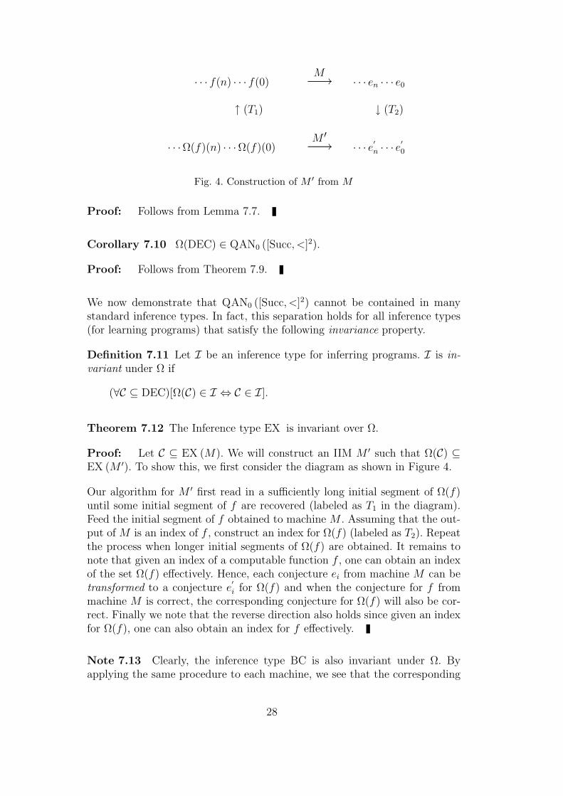
Fig. 4. Construction of M ′ from M
Proof: Follows from Lemma 7.7.
Corollary 7.10 Ω(DEC) ∈ QAN0 ([Succ, <]2).
Proof: Follows from Theorem 7.9.
We now demonstrate that QAN0 ([Succ, <]2) cannot be contained in manystandard inference types. In fact, this separation holds for all inference types(for learning programs) that satisfy the following invariance property.
Definition 7.11 Let I be an inference type for inferring programs. I is in-variant under Ω if
(∀C ⊆ DEC)[Ω(C) ∈ I ⇔ C ∈ I].
Theorem 7.12 The Inference type EX is invariant over Ω.
Proof: Let C ⊆ EX (M). We will construct an IIM M ′ such that Ω(C) ⊆EX (M ′). To show this, we first consider the diagram as shown in Figure 4.
Our algorithm for M ′ first read in a sufficiently long initial segment of Ω(f)until some initial segment of f are recovered (labeled as T1 in the diagram).Feed the initial segment of f obtained to machine M . Assuming that the out-put of M is an index of f , construct an index for Ω(f) (labeled as T2). Repeatthe process when longer initial segments of Ω(f) are obtained. It remains tonote that given an index of a computable function f , one can obtain an indexof the set Ω(f) effectively. Hence, each conjecture ei from machine M can betransformed to a conjecture e
′i for Ω(f) and when the conjecture for f from
machine M is correct, the corresponding conjecture for Ω(f) will also be cor-rect. Finally we note that the reverse direction also holds since given an indexfor Ω(f), one can also obtain an index for f effectively.
Note 7.13 Clearly, the inference type BC is also invariant under Ω. Byapplying the same procedure to each machine, we see that the corresponding
28
Fig. 5. Sample Comparison Results with variants of EX
team’s types are also invariant under Ω. The invariance of these inference typesare also preserved when we restrict the number of mindchanges. Therefore,the combinations such as [a, b]EXm (a ≥ b ≥ 1,m ≥ 0) and etc. are allinvariant under Ω. However, it is unclear if the inference types with anomaliesare invariant under Ω.
Theorem 7.14 Let I be invariant under Ω. Then
(∀L ≤N [Succ, <]2)[DEC 6∈ I ⇒ QAN0 (L) 6⊆ I].
Proof: Since I is invariant under Ω, DEC 6∈ I ⇒ Ω(DEC) 6∈ I. How-ever, it follows from Theorem 7.9 that Ω(DEC) ∈ QAN0 ([Succ, <]2). Hence,Ω(DEC) ∈ QAN0 ([Succ, <]2)−I. The general case follows from Lemma 2.14.
Corollary 7.15 Let L ≤N [Succ, <]2 and i, j ∈ N ∪ ∗ (i 6= 0). Suppose Iis invariant under Ω. Then DEC 6∈ I ⇒ QiANj (L) 6⊆ I.
Proof: By Theorem 7.14 and the fact that QAN0 (L) ⊆ QiANj (L).
By the remarks stated in Note 7.13 and prior results, we can visualize thedifference between the learning of answers and the learning of programs (SeeFigure 5 for sample comparison results with variants of EX). In fact, we have
Corollary 7.16
(1) L ≤N [Succ, <]2 ⇒ (∀n ≥ 1)[QAN0 (L) 6⊆ [1, n]BC].(2) For all b, (∀n ≥ 1)[QAN0 [+, <,POWb] 6⊆ [1, n]BC].
29
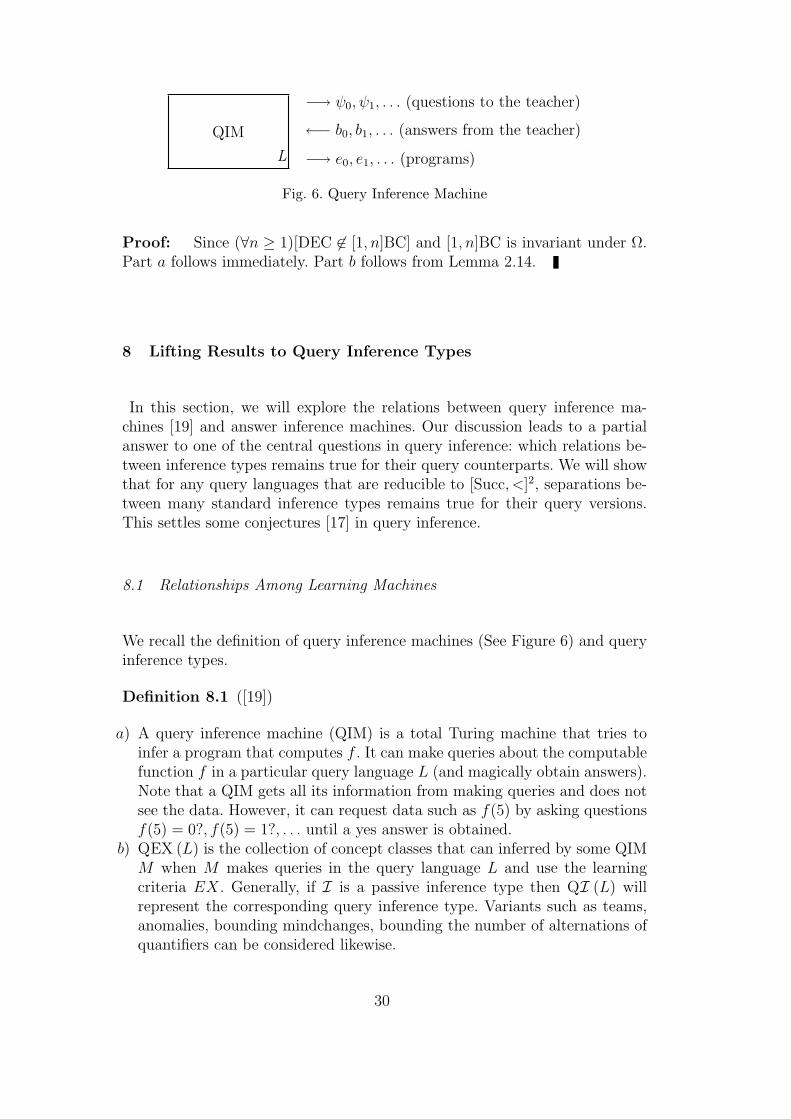
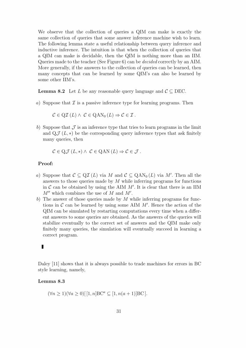
QIM
−→ ψ0, ψ1, . . . (questions to the teacher)
−→ e0, e1, . . . (programs)
←− b0, b1, . . . (answers from the teacher)
L
Fig. 6. Query Inference Machine
Proof: Since (∀n ≥ 1)[DEC 6∈ [1, n]BC] and [1, n]BC is invariant under Ω.Part a follows immediately. Part b follows from Lemma 2.14.
8 Lifting Results to Query Inference Types
In this section, we will explore the relations between query inference ma-chines [19] and answer inference machines. Our discussion leads to a partialanswer to one of the central questions in query inference: which relations be-tween inference types remains true for their query counterparts. We will showthat for any query languages that are reducible to [Succ, <]2, separations be-tween many standard inference types remains true for their query versions.This settles some conjectures [17] in query inference.
8.1 Relationships Among Learning Machines
We recall the definition of query inference machines (See Figure 6) and queryinference types.
Definition 8.1 ([19])
a) A query inference machine (QIM) is a total Turing machine that tries toinfer a program that computes f . It can make queries about the computablefunction f in a particular query language L (and magically obtain answers).Note that a QIM gets all its information from making queries and does notsee the data. However, it can request data such as f(5) by asking questionsf(5) = 0?, f(5) = 1?, . . . until a yes answer is obtained.
b) QEX (L) is the collection of concept classes that can inferred by some QIMM when M makes queries in the query language L and use the learningcriteria EX. Generally, if I is a passive inference type then QI (L) willrepresent the corresponding query inference type. Variants such as teams,anomalies, bounding mindchanges, bounding the number of alternations ofquantifiers can be considered likewise.
30
We observe that the collection of queries a QIM can make is exactly thesame collection of queries that some answer inference machine wish to learn.The following lemma state a useful relationship between query inference andinductive inference. The intuition is that when the collection of queries thata QIM can make is decidable, then the QIM is nothing more than an IIM.Queries made to the teacher (See Figure 6) can be decided correctly by an AIM.More generally, if the answers to the collection of queries can be learned, thenmany concepts that can be learned by some QIM’s can also be learned bysome other IIM’s.
Lemma 8.2 Let L be any reasonable query language and C ⊆ DEC.
a) Suppose that I is a passive inference type for learning programs. Then
C ∈ QI (L) ∧ C ∈ QAN0 (L)⇒ C ∈ I .
b) Suppose that J is an inference type that tries to learn programs in the limitand QJ (L, ∗) be the corresponding query inference types that ask finitelymany queries, then
C ∈ QJ (L, ∗) ∧ C ∈ QAN (L)⇒ C ∈ J .
Proof:
a) Suppose that C ⊆ QI (L) via M and C ⊆ QAN0 (L) via M ′. Then all theanswers to those queries made by M while inferring programs for functionsin C can be obtained by using the AIM M ′. It is clear that there is an IIMM ′′ which combines the use of M and M ′.
b) The answer of those queries made by M while inferring programs for func-tions in C can be learned by using some AIM M ′. Hence the action of theQIM can be simulated by restarting computations every time when a differ-ent answers to some queries are obtained. As the answers of the queries willstabilize eventually to the correct set of answers and the QIM make onlyfinitely many queries, the simulation will eventually succeed in learning acorrect program.
Daley [11] shows that it is always possible to trade machines for errors in BCstyle learning, namely,
Lemma 8.3
(∀n ≥ 1)(∀a ≥ 0)[ [1, n]BCa ⊆ [1, n(a+ 1)]BC ].
31
Hence Corollary 7.16 can be further improved even though the inference type[1, n]QBCa (L) may not be invariant under Ω.
Theorem 8.4 Let a, n ∈ N and n ≥ 1. Then
QAN0 ([Succ, <]2) 6⊆ [1, n]QBCa ([Succ, <]2)
Proof: Assume by way of contradiction that
QAN0 ([Succ, <]2) ⊆ [1, n]QBCa ([Succ, <]2),
where a, n ∈ N (n 6= 0). Hence we have (QAN0 ([Succ, <]2) ⊆ QAN0 ([Succ, <]2)) ∧ (QAN0 ([Succ, <]2) ⊆ [1, n]QBCa ([Succ, <]2)).
By Lemma 8.2, we obtain
QAN0 ([Succ, <]2) ⊆ [1, n]BCa .
In addition, by trading machines for errors (Lemma 8.3) we get
QAN0 ([Succ, <]2) ⊆ [1, n(a+ 1)]BC .
By Corollary 7.10 Ω(DEC) ∈ QAN0 ([Succ, <]2), hence Ω(DEC) ∈ [1, n(a +1)]BC . Since [1, n(a + 1)]BC is invariant under Ω, DEC ∈ [1, n(a + 1)]BC ,which is a contradiction (See [9]).
Corollary 8.5 Given a query language L,
L ≤N [Succ, <]2 ⇒ (∀n ≥ 1)(∀a ∈ N)[QAN0 (L) 6⊆ [1, n]QBCa (L)].
Proof: Use reduction in Corollary 8.4.
Note 8.6 We use only the fact that (∀a ∈ N)[DEC 6∈ [1, a]BC]. Hence weobtain a short proof of the result ([17])
L ≤N [Succ, <]2 ⇒ (∀n ≥ 1)(∀a ∈ N)[DEC 6∈ [1, n]QBCa (L)].
8.2 A Lifting Lemma
32
Lemma 8.7 Let I be a passive inference type that is invariant under Ω. Then
A ∈ QI ([Succ, <]2) iff A ∈ I.
Proof: Assume A ∈ QI ([Succ, <]2). By Lemma 7.7 we can take the query-inference procedure for A and turn it into a passive-inference procedure forΩ(A). Hence Ω(A) ∈ I. Since I is invariant we have A ∈ I.
It is clear that if A ∈ I then A ∈ QI ([Succ, <]2).
Theorem 8.8 Let I, J be two passive inference types and QI (L), QJ (L)be the corresponding query inference types. Suppose I and J are invariantunder Ω. Then
J − I 6= ∅ ⇒ J −QI ([Succ, <]2) 6= ∅.
Proof: Suppose J − I 6= ∅. Hence there exists C ⊆ DEC such that C ∈J − I. By Lemma 8.7, C /∈ QI ([Succ, <]2). Hence J − QI ([Succ, <]2) 6= ∅.
The following theorem is proven by a sight modification of Theorem 8.8
Theorem 8.9 Let I, J be two passive inference types and QI (L), QJ (L)be the corresponding query inference types. Suppose I and J are invariantunder Ω. Let L ≤N [Succ, <]2. Then
J − I 6= ∅ ⇒ J −QI (L) 6= ∅.
Note 8.10 For many passive inference types I and J and languages L, theinclusion QI (L) ⊆ QJ (L) follows immediately from the proof of the inclu-sion I ⊆ J . Hence, for such cases we actually have
I ⊂ J ⇒ QI (L) ⊂ QJ (L).
Theorem 8.9 helps to lift separation results to their query versions. For in-stance, Smith [30] shows that
Theorem 8.11 ( [30])
EX ⊂ [1, 2]EX ⊂ [1, 3]EX ⊂ · · · and BC ⊂ [1, 2]BC ⊂ [1, 3]BC ⊂ · · ·
All these inference types are invariant under Ω. Therefore we have the followingcorollary, which settles a few questions raised in [17,20].
33
Corollary 8.12 Let L ≤N [Succ, <]2. Then
a) QEX (L) ⊂ [1, 2]QEX (L) ⊂ [1, 3]QEX (L) ⊂ · · ·b) QBC (L) ⊂ [1, 2]QBC (L) ⊂ [1, 3]QBC (L) ⊂ · · ·
Proof:
QEX (L) ⊆ [1, 2]QEX (L) ⊆ [1, 3]QEX (L) ⊆ · · ·
and
QBC (L) ⊆ [1, 2]QBC (L) ⊆ [1, 3]QBC (L) ⊆ · · ·
follows directly from their definitions. It suffices to note that by applying liftinglemma (Theorem 8.9) to Theorem 8.11, the non-inclusion follows immediately.
Interestingly, we also have an analogue of the ‘[24, 49]’ Theorem [12] for queryinference types.
Corollary 8.13 Let L ≤N [Succ, <]2. Let c, d be such that 24/49 < c/d <1/2. Then
a) [1, 2]QEX0 (L) ⊂ [2, 4]QEX0 (L) ⊂ [24, 49]QEX0 (L).b) [24, 49]QEX0 (L)− [c, d]QEX0 (L) 6= ∅.
Proof:
a) It is easy to see that
[1, 2]QEX0 (L) ⊆ [2, 4]QEX0 (L) ⊆ [24, 49]QEX0 (L).
By applying the lifting lemma (Theorem 8.9) to the results ([12])
[2, 4]EX0 − [1, 2]EX0 6= ∅
and
[24, 49]EX0 − [2, 4]EX0 6= ∅,
we have
[1, 2]QEX0 (L) ⊂ [2, 4]QEX0 (L) ⊂ [24, 49]QEX0 (L).
b) By applying the lifting lemma (Theorem 8.9) to the following result [12]
[24, 49]EX0 − [c, d]EX0 6= ∅
34
we have
[24, 49]QEX0 (L)− [c, d]QEX0 (L) 6= ∅
Corollary 8.14
a) For all b,
QEX ([+, <,POWb])⊂ [1, 2]QEX ([+, <,POWb])⊂ [1, 3]QEX ([+, <,POWb])⊂ [1, 4]QEX ([+, <,POWb]) ⊂ · · ·
b) For all b,
QBC ([+, <,POWb])⊂ [1, 2]QBC ([+, <,POWb])⊂ [1, 3]QBC ([+, <,POWb])⊂ [1, 4]QBC ([+, <,POWb]) ⊂ · · ·
c) Let b ∈ N. Let c, d ∈ N be such that 24/49 < c/d < 1/2. Then
[1, 2]QEX0 ([+, <,POWb]) ⊂ [2, 4]QEX0 ([+, <,POWb])
⊂ [24, 49]QEX0 ([+, <,POWb])
and [24, 49]QEX0 ([+, <,POWb])− [c, d]QEX0 ([+, <,POWb]) 6= ∅.
Proof: This follows from Corollaries 8.12, 8.13, and Fact 2.12.
9 Open Problems
Query languages: The results in this work holds for languages that are re-ducible to [Succ, <]2. Our techniques depend on decidability results fromthe theory of omega automata. Do these results still hold for any querylanguages with a decidable base languages?
Lifting separations: We proved a lifting lemma which ‘lifts’ every separa-tions to their query inference analogue when no anomalies are involved. Willthe lifting lemma hold when anomalies are allowed ?
Lifting subset relations: Can subset relations be also lifted? For example,can one show the following:
(∀L ≤N [Succ, <]2)(∀a, b, c, d ∈ N)
[a, b]EX0 ⊆ [c, d]EX0 ⇒ [a, b]QEX0 (L) ⊆ [c, d]QEX0 (L)
35
Acknowledgment: We thank We thank Kalvis Apsitis, John Case, MarkChangizi, Lazaros Kikas, April Lee, Georgia Martin, and Frank Stephan forproofreading. We thank John Case, Jim Royer, and Frank Stephan for discus-sion of the primitive recursive recursion theorem.
References
[1] J. Buchi. Weak second order arithmetic and finite automata. Zeitsch. f. math.Logik und Grundlagen d. Math., 6:66–92, 1960.
[2] J. Buchi. On a decision method in restricted second order arithmetic. InE. Nagel et al., editors, Logic Methodology and Philosophy of Science, pages 1–11. Stanford University Press, 1962.
[3] D. Angluin and C. Smith. Inductive inference: Theory and methods. ComputingSurveys, 15:237–269, 1983.
[4] G. Baliga, J. Case, S. Jain, and M. Suraj. Machine learning on higher-orderprograms. The Journal of Symbolic Logic, 59(2):486–500, 1994.
[5] Ben-David. Can finite samples detect singularities. Algorithmica, 22, 1998.Prior version in STOC92.
[6] L. Blum and M. Blum. Toward a mathematical theory of inductive inference.Information and Control, 28:125–155, 1975.
[7] J. Case, S. Jain, and A. Sharma. On learning limiting programs. Internat. J.Found. Comput. Sci, 3(1):93–115, 1992.
[8] J. Case, E. Kinber, A. Sharma, and F. Stephan. On the classification ofcomputable languages. Information and Computation, 192, 2004.
[9] J. Case and C. Smith. Comparison of identification criteria for machineinductive inference. Theoretical Computer Science, 25:193–220, 1983.
[10] Y. Choueka. Theory of automata on ω-tapes. Journal of Computer and SystemSciences, 8:117–142, 1974.
[11] R. Daley. On the error correcting power of pluralism in bc-type inductiveinference. Theoretical Computer Science, 24(1):95–104, 1983.
[12] R. Daley, B. Kalyanasundaram, and M. Velauthapillai. Breaking the probability1/2 barrier in fin-type learning. Journal of Computer and System Sciences,50:574–599, 1995.
[13] M. Davis. Hilbert’s 10th problem is unsolvable. Amer. Math. Monthly, 80:233–269, 1973.
[14] M. Davis, P. H., and R. J. The decision problem of exponential diophantineequations. Ann. math., 74:425–436, 1961.
36
[15] C. Elgot and M. O. Rabin. Decidability and undecidability of extensions ofsecond (first) order theory of (generalized) successor. The Journal of SymbolicLogic, 31:169–181, 1966.
[16] H. B. Enderton. A mathematical introduction to logic. Academic Press, 1972.
[17] W. Gasarch and G. Hird. Automata techniques for query inference machines.Annals of pure and applied logic, 117:171–203, 2002. Prior version inComputational Learning Theory, 1995 (COLT).
[18] W. Gasarch, M. Pleszkoch, and R. Solovay. Learning via queries in [+, <].Journal of Symbolic Logic, 57:58–81, 1992.
[19] W. Gasarch and C. Smith. Learning via queries. Journal of ACM, 39:649–676,1992.
[20] W. Gasarch and C. H. Smith. A survey of inductive inference with an emphasison queries. In A. Sorbi, editor, Complexity, Logic, and Recursion Theory,number 187 in Lecture notes in Pure and Applied Mathematics Series. M.Dekker., 1997.
[21] W. I. Gasarch, M. G. Pleszkoch, F. Stephan, and M. Velauthapillai.Classification using information. Annals of mathematics and artificialintelligence, 23(1-2), 1998. Earlier version in ALT94.
[22] E. Gold. Language identification in the limit. Information and Control, 10:447–474, 1967.
[23] S. Jain, D. Osherson, J. Royer, and A. Sharma. Systems that Learn: AnIntroduction to Learning Theory for Cognitive and Computer Scientists. M.I.T.Press, 1999.
[24] K. T. Kelly. The logic of reliable inquiry. Logic and Computation in Philosophy.The Clarendon Press Oxford University Press, New York, 1996.
[25] Y. V. Matiyasevich. Enumerable sets are diophantine. Doklady Academy Nauk.SSSR, 191:279–282, 1970. Translation in Sov. Math. Dokl. 11 (1970), 354-357.
[26] Y. V. Matiyasevich. Hilbert’s tenth problem. Foundations of Computing Series.MIT Press, Cambridge, MA, 1993. Translated from the 1993 Russian originalby the author, With a foreword by Martin Davis.
[27] M. Rabin. Decidable theories. In J. Barwise, editor, Handbook of MathematicalLogic. North Holland, 1977.
[28] J. Royer and J. Case. Subrecursive Programming Systems: Complexity andSuccinctness. Birkhauser, 1994.
[29] D. Siefkes and J. R. Buchi. The monadic second order theory of all countableordinals. In G. Muller and D. Siefkes, editors, Decidable Theories II, volume328 of Lecture Notes in Mathematics. Springer Verlag, New York, 1973.
[30] C. Smith. The power of pluralism for automatic program synthesis. Journal ofACM, 29(4):1144–1165, 1982.
37

[31] C. Smith, R. Wiehagen, and T. Zeugmann. Classification of predicates andlanguages. In Computational learning theory : EuroCOLT ’93, pages 171–181.Oxford University Press, 1994.
[32] C. H. Smith. A Recursive Introduction of Theory of Computation. SpringerVerlag, 1994.
[33] C. H. Smith and R. Wiehagen. Generalization versus classification. Journal ofExperimental and Theoretical Artificial Intelligence, 7:163–174, 1995.
[34] R. Soare. Recursively Enumerable Sets and Degrees. Omega Series. Springer-Verlag, 1987.
[35] F. Stephan. Learning via queries and oracles. Annals of Pure and AppliedLogic, 94:273–296, 1998. Prior version in Computational Learning Theory, 1995(COLT).
[36] W. Thomas. Automata on infinite objects. In J. V. Leeuwen, editor, Handbookof Theoretical Computer Science, volume 2, chapter 4, pages 135 –191. ElsevierScience Publishers B.V., 1990.
[37] W. Thomas. Language, automata and logic. In G. Rozenberg and A. Salomaa,editors, Handbook of Formal Languages Vol.3 BEYOND WORDS, pages 389–455. Spring Verlag, 1997.
38