Embed Size (px)
Citation preview
Explaining Query Answerswith Explanation-Ready Databases
Sudeepa Roy∗
Duke University
Laurel OrrUniversity of Washington
Dan SuciuUniversity of Washington
ABSTRACTWith the increased generation and availability of big datain different domains, there is an imminent requirement fordata analysis tools that are able to ‘explain’ the trendsand anomalies obtained from this data to a range of userswith different backgrounds. Wu-Madden (PVLDB 2013)and Roy-Suciu (SIGMOD 2014) recently proposed solutionsthat can explain interesting or unexpected answers to sim-ple aggregate queries in terms of predicates on attributes.In this paper, we propose a generic framework that can sup-port much richer, insightful explanations by preparing thedatabase offline, so that top explanations can be found inter-actively at query time. The main idea in such explanation-ready databases is to pre-compute the effects of potential ex-planations (called interventions), and efficiently re-evaluatethe original query taking into account these effects. Weformalize this notion and define an explanation-query thatcan evaluate all possible explanations simultaneously with-out having to run an iterative process, develop algorithmsand optimizations, and evaluate our approach with experi-ments on real data.
1. INTRODUCTIONWith the increased generation and availability of large
amounts of data in different domains, a range of users, e.g.,data analysts, domain scientists, marketing specialists, de-cision makers in industry, and policy makers in the publicsector intend to analyze such data on a regular basis. Theyexplore these datasets using modern tools and interfaces fordata visualization, then try to understand the trends andanomalies they observed in their exploration so that appro-priate actions can be taken. However, there are currentlyno tools available that can automatically ‘explain’ trendsand anomalies in data. As more users interact with moredatasets, the need for such tools will only increase.
∗This work was done while the author was at the Universityof Washington.
This work is licensed under the Creative Commons Attribution-NonCommercial-NoDerivatives 4.0 International License. To view a copyof this license, visit http://creativecommons.org/licenses/by-nc-nd/4.0/. Forany use beyond those covered by this license, obtain permission by [email protected] of the VLDB Endowment, Vol. 9, No. 4Copyright 2015 VLDB Endowment 2150-8097/15/12.
A couple of recent research projects by Wu and Madden[34] and Roy and Suciu [32] have proposed techniques forexplaining interesting or unexpected answers (e.g., outliers)to a query Q on a database D. For instance: why is theaverage temperature reported by a number of sensors be-tween 12PM and 1PM unexpectedly high [34]?, or, why doesthe number of SIGMOD publications from industry have apeak during the early years of the 21st century [32]? Both[34] and [32] consider an explanation to be a conjunctivepredicate on the input attributes, e.g., [sensorid = 18], or[author.institution = ’Oxford’ and paper.year = ’2002’].An explanation predicate is considered good for a particu-lar trend or outlier if, by removing from the database alltuples that ‘depend on’ the predicate, the trend changes orthe outlier is eliminated. In the sensor data example, theexplanation [sensorid = 18] means that, if we removed allreadings from this sensor, then the average temperature be-tween 12PM and 1PM is no longer high. We give a newexample in this paper from the NSF awards dataset1.
Example 1.1. The three main tables in the NSF awardsdataset are as follows (the keys are underlined):
Award(aid, amount, title, year, startdate, enddate, dir, div);
Institution(aid, instName, address);
Investigator(aid, PIName, emailID)
Here dir denotes the directorate, i.e., the area like ComputerScience (CS), and div is the division within an area, e.g.,CCF, CNS, IIS, ACI for CS. Now consider the query below:
SELECT TOP 5 B.instName, SUM(A.amount) AS totalAward
FROM Award A, Institution B
WHERE A.aid = B.aid AND dir = ’CS’ AND year >= 1990
GROUP BY B.instName
ORDER BY totalAward DESC
The above query seeks the top-5 institutions with thehighest total award amount in CS from 1990, and producesthe following answer:
instName totalAwardUniversity of Illinois at Urbana-Champaign 1,169,673,252University of California-San Diego 723,335,212Carnegie-Mellon University 472,915,775University of Texas at Austin 319,437,217Massachusetts Institute of Technology 292,662,491
1This publicly available dataset [1] contains awards from1960 to 2014 in XML that we converted into relations. Weomit some tables and attributes, and use abbreviations forsimplicity, e.g., the directorate of CS will appear as ‘Direc-torate for Computer & Information Science & Engineering’.
348
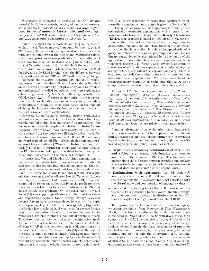
If someone is interested in analyzing the NSF fundingawarded to different schools, looking at the above answers,she might try to understand ‘why there is a huge differ-ence in award amounts between UIUC and CMU’, espe-cially given that CMU holds rank-1 as a CS graduate schooland UIUC holds rank-5 (according to US News [2]).
Indeed, the algorithms in both [34] and [32] can be used toexplain the difference in award amounts between UIUC andCMU; since [34] operates on a single relation, it will first ma-terialize the join between the Award and Institution tables.Both the approaches return predicates on the attributes ofthese two tables as explanations, e.g., [div = ’ACI’] (Ad-vanced Cyberinfrastructure). Intuitively, if the awards fromthis division are removed (which amounts to about $893Mfor UIUC and only $26M for CMU), then the difference betweenthe award amounts for UIUC and CMU will drastically change.
Following the causality literature [29], the act of remov-ing tuples from a database D and then studying its effecton the answer to a query Q (not physically, only to evaluatean explanation) is called an intervention. An explanatione has a high score if Q[D − ∆De] differs significantly fromQ[D], where ∆De ⊆ D refers to the tuples in the interven-tion of e. An explanation system considers many candidateexplanations e, computes some score based on the amountof change in the query after the intervention, and returns tothe user a ranked list of explanations.
However, for performance reasons, current explanationsystems severely limit the types of explanations that theysearch, and fail to find deep and insightful explanations. Forinstance, an interesting explanation is the PI ‘Robert Pen-nington’, who received more than $580M for UIUC in CS.His absence from the database will hugely affect the differ-ence between the award amounts of UIUC and CMU (assumingan award depends on all PIs). Although this explanation isexpressible as a predicate [PIName = ’Robert Pennington’],both [34, 32] fail to return this explanation simply becausethe PI information belongs to the third table Investigator,which does not appear in the query in Example 1.1.
In particular, Wu and Madden [34] limit explanations topredicates on a single table (base relation or a material-ized result), thereby possibly missing explanations that de-pend on mutual dependency of multiple tables in a database.Even if all three tables are joined and materialized a pri-ori, the intervention of predicates like [PIName = ’RobertPennington’] (removal of all awards for this PI) cannot becomputed by removing tuples satisfying the predicate, sincethere will be other rows for awards with multiple PIs thatdo not satisfy this predicate. On the other hand, Roy andSuciu [32] can support predicates spanning multiple tablesand dependency between tables through foreign keys andreverse foreign keys as causal dependencies — if a tuplewith a primary key is deleted, the corresponding tuple withthe foreign key is deleted (and vice versa for reverse foreignkeys). But computing the effect of an intervention, in theworst case, requires running a non-trivial recursive query.Therefore, they restrict the predicates to conjunctive equal-ity predicates on the tables used in the query so that theefficient OLAP data cube operation in SQL can be used toincrease performance. Moreover, both [34] and [32] restrictthe class of input queries to single-block aggregate queries(of the form select-from-where-group by as in Example 1.1)without any nested sub-queries, which cannot express someimportant statistical methods frequently used in data anal-
ysis (e.g., linear regression or correlation coefficient on in-termediate aggregates, an example is given in Section 5).
In this paper we propose a new approach for finding deep,semantically meaningful explanations with interactive per-formance, which we call Explanation-Ready Databases(ERD). Our proposal is based on two ideas. First, we pre-compute the interventions associated with a large numberof potential explanations and store them in the database.Note that the intervention is defined independently of aquery, and therefore it can be precomputed. We use ar-bitrary causal dependencies induced by the semantic of theapplication to associate interventions to candidate explana-tions (ref. Section 3.1). Second, at query time, we computethe scores of all candidate explanations simultaneously, bya single SQL query called the explanation-query, which isevaluated on both the original data and the interventionsassociated to all explanations. We present a suite of in-cremental query computation techniques that allow us tocompute the explanation query at an interactive speed.
Example 1.2. For the explanation e ∶ [PIName =’Robert Pennington’], ∆De = (∆Award,e, ∆Institution,e,∆Investigator,e) consists of interventions on all three tables.PIs do not affect the presence of their institutions in thedatabase, therefore ∆Institution,e = ∅. ∆Investigator,e containsall tuples from Investigator such that PIName = ’RobertPennington’ and ∆Award,e contains all awards with ‘RobertPennington’ as a PI. ∆Award can be populated with interven-tions of all such explanations e (indexed by e) by a nestedSQL query that joins the Award and Investigator tables.
A major advantage of an explanation-ready database isthat it can consider much richer explanations of differentforms, because the high cost of computing their interventionis paid offline (e.g., by running multi-block SQL queries withnested aggregates and joins). Examples include:
● Explanations involving combination of attributesand tables: e.g., awards with duration ≥ x years orawards with the number of PIs ≥ y. The first one re-quires taking the difference between startdate and enddatewhereas the latter requires a join with the Investigator ta-ble that does not participate in the original query.
● Explanations with aggregates: e.g., PIs with ≥ Xawards, ≥ Y co-PIs, or ≥ Z total award amount. Thisrequires joining the Investigator table with itself or withthe Award table and computation of aggregate values.
● Explanations having top-k form: If one or more fromthe top-k PI-s (according to total award amount, averageaward amount, etc.) across all institutions belong to UIUC,they can explain the high award amounts of UIUC.
To improve the performance of the explanation querywe adapt techniques from Incremental View Maintenance(IVM). In Section 2, we discuss the similarities and differ-ences between IVM and an ERD. Specifically, our task is tocompute Q[D−∆De] incrementally, from Q[D] for all e. InIVM, the goal is to re-compute a given query when a singletuple is deleted from the database, or a subset of tuples forbatch deletion. In our case, (i) the query is only known atruntime, and (ii) not only the intervention ∆De containsmany tuples from many relations, there can be thousandsof such ∆De-s; in fact, the union of all ∆De-s for all candi-date explanations e can be much larger than the database D,
349
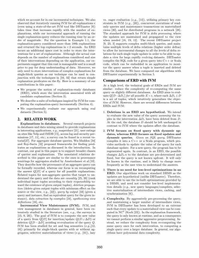
which we account for in our incremental techniques. We alsoobserved that iteratively running IVM for all explanations e(even using a state-of-the-art IVM tool like DBToaster [9])takes time that increases rapidly with the number of ex-planations, while our incremental approach of running thesingle explanation-query reduces the running time by an or-der of magnitude. For the question in Example 1.1, theexplanation-query considered more than 188k explanationsand returned the top explanations in < 2 seconds. An ERDincurs an additional space cost in order to store the inter-ventions for a set of explanations. Although the actual costdepends on the number of explanations considered and sizeof their interventions depending on the application, our ex-periments suggest that this cost is manageable and is a smallprice to pay for deep understanding of data. Moreover, weonly need to store interventions of complex explanations forsingle-block queries as our technique can be used in con-junction with the techniques in [34, 32] that return simpleexplanation predicates on the fly. Here is a summary of ourcontributions in this paper:
● We propose the notion of explanation-ready databases(ERD), which store the intervention associated with allcandidate explanations (Section 3).
● We describe a suite of techniques inspired by IVM for com-puting the explanation-query incrementally (Section 4).
● We experimentally evaluate our approach using realdatasets (Section 5).
2. RELATED WORKExplanations in databases. Several research projects
in databases and data mining aimed to provide explanationsin interesting applications, e.g., mapreduce [21], user ratingson sites like Yelp and IMDB [15], access log and security per-missions [17, 11], etc.; a survey can be found in a recent tu-torial[27]. For aggregate database queries, Wu-Madden [34]and Roy-Suciu [32] proposed frameworks for finding pred-icates as explanations as discussed in the introduction. Incontrast, our goal in this paper is to support broader classesof queries and explanations. The annotated relations de-scribed in this paper are similar to the ones in provenancesemirings for aggregates studied by Amsterdamer et al.[10].They describe how the provenance of an aggregate query canbe formally recorded, whereas our focus is on recomputingthe answer Q[D] of a query for all possible explanations.Related topics for non-aggregate queries that target to un-derstand the query and the data are causality [25, 26] (rankindividual input tuples according to their responsibility to-ward the existence of given output tuples), deletion propaga-tion (delete given output tuples with minimum effect on thesource or the view, e.g., [22]), query by output [33] (given aquery and instance, find an equivalent query for the given in-stance), data extraction by examples [24], synthesizing viewdefinitions [16], etc.
Incremental View Maintenance (IVM). IVM, andview management in databases in general, have been ex-tensively studied in the literature (see, e.g., the surveys in[13, 9, 20]). The goal of IVM is to compute the new valueof a query from Q[D] for insertion/update Q(D ∪ ∆D) ordeletion Q[D −∆D] avoiding re-evaluation of the query Q.IVM has been studied for set and bag semantics (e.g.,[12,18]) primarily for single-block queries with or without ag-gregates, selective materialization of views (e.g., [31]), lazy
vs. eager evaluation (e.g., [14]), utilizing primary key con-straints in IVM (e.g., [20]), concurrent executions of read-only queries and maintenance transactions on materializedviews [30], and for distributed programs in a network [28].The standard approach for IVM is delta processing, wherethe updates are maintained and propagated to the viewwhen needed [18, 19, 12]. The recent DBToaster project[9, 23, 3] supports complex multi-block queries, and main-tains multiple levels of delta relations (higher order deltas)to allow for incremental changes to all the levels of delta re-lations for each single tuple update in order to be able to up-date a view for large rapidly evolving datasets. DBToastercompiles the SQL code for a given query into C++ or Scalacode, which can be embedded in an application to moni-tor the query answer when a tuple is inserted and deletedfrom the database. We have compared our algorithms withDBToaster experimentally in Section 5.
Comparisons of ERD with IVMAt a high level, the technical goals of ERDs and IVM aresimilar: reduce the complexity of re-computing the samequery on slightly different databases. An ERD aims to eval-uate Q[D−∆De] for all possible E = e, where each ∆De ⊆Dis a set of tuples, which intuitively generalizes the objec-tive of IVM. However, there are several differences betweenERDs and IVM:
1. Deletions in an ERD are hypothetical. We intendto evaluate the new value of the query assuming the tu-ples in the intervention ∆De have been deleted from D.At the end, the database D should be left unchanged incontrast to IVM where the updates affect the database.
2. IVM focuses on fixed query with dynamic up-dates, whereas ERD focuses on fixed updates anddynamic queries. Given an SQL query, DBToastercompiles it into a C++ or a Scala program, which pro-vides methods to update the value of the query for eachdatabase update. For a new query, the program has to beregenerated again. In contrast, in an ERD, the possiblechanges ∆De-s to the database are pre-determined andfixed, but the query is not known upfront. It will onlybe known in the runtime, and is likely to change morefrequently as the user tries to understand the answers.
3. There is no need for low-level optimizations in anERD. Our algorithms work on standard DBMS as theupdates are hypothetical (unlike DBToaster). Therefore,we are able to use the in-built optimizations provided bya DBMS, and need not consider low-level implementa-tion details (e.g., new query languages/compilers, selec-tive materialization of intermediate views, caching, andsynchronization [9]).
4. Complexity. By aggressively pre-processing the query,and maintaining a larger number of intermediate views,IVM in DBToaster has been developed to an extremesuch that every update to a materialized view can be com-puted in NC0 (Koch [23]). In the explanation framework,the query is only known at runtime, and as a consequencewe cannot perform a similar aggressive preprocessing. In-stead, we reduce the complexity from re-computing thesame query once for each intervention, to computing asingle query over a larger database. In general, our algo-rithms have polynomial data complexity.
350
The main focus of an ERD is to compute Q[D−∆De] for allE = e without having to run an iterative ‘for loop’ on suche-s, which is orthogonal to the goal of the IVM approaches.Our experiments in Section 5 show that iteratively runningIVM (e.g., DBToaster) for all E = e does not give good per-formance. Nevertheless, due to the simililarity with the highlevel goal of IVM, our techniques are motivated by the IVMliterature. For instance, the update rules in Section 4.3 canbe considered as extensions to the update rules in IVM [12,18], although these rules take into account multiple updatesto the views for all explanations E = e simultaneously, andtherefore incur additional complexity (e.g., the union of the∆De relations can be much larger than the original databaseD in an ERD, which is never the case for IVM).
3. EXPLANATION-READY DATABASESWe describe here the framework for an explanation-ready
database (ERD). The offline part is discussed in Section 3.1,and the interactive part in Section 3.2.
3.1 Preparing the DatabaseAn explanation-ready database ERD(D,P,T ,E) (ERD in
short) has four components:
● A standard relational database D with k relationsD = (S1,⋯, Sk) for some constant k ≥ 1. The relation Si
has attributes Ai for2 i ∈ [1, k].
● A set of explanation types T ; each type has an identi-fier, a short English description, and k SQL queries (onefor each relation Si, discussed below).
● A class of potential explanations (henceforth, explana-tions) E , where each explanation (e,∆De,typee) ∈ E hasthree components:
1. ID: A unique integer identifier e.
2. Intervention: A subset of tuples ∆De =
(∆1,e,⋯,∆k,e); each ∆i,e ⊆ Si, i ∈ [1, k]. By in-tervening the explanation e, we mean removing alltuples ∆De from the database D.
3. Type: A typee ∈ T .
● A set of causal dependencies P among tuples usingdatalog rules (described below).
The ERD is prepared offline, independently of any query,and stored in the databases as follows. There is a separatetable storing the types in T . All explanations are storedtogether in k tables, denoted ∆D = (∆1,⋯,∆k), where ∆i
has the same attributes as the relation Si plus an extra at-tribute E, storing the explanation identifier e; thus, for eachidentifier value e, one can recover the intervention associ-ated to e, ∆i,e, through a selection followed by a projection:∆i,e = πAi
σE=e∆i. We also create a primary index (non-unique) on the attribute E. Finally, we store separately themany-one relationship associating each explanation identi-fier e with its type. Here is a toy example:
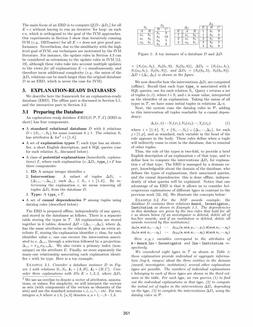
Example 3.1. Consider a database instance D in Fig-ure 1 with relations S1, S2, A1 = {A,B}, A2 = {B,C}. Con-sider three explanations with IDs E = 1,2,3, where ∆D1
2 We use an overline to denote a vector of attributes, annota-tions, or values; For simplicity, we will interpret the vectorsas sets (with components of the vectors as elements of thesets) and use the standard notations ∈,⊆,∪,∩,∖ etc. For twointegers a, b where a ≤ b, [a, b] denotes a, a + 1,⋯, b − 1, b.
S1
A Ba1 b1a1 b2a2 b1
S2
B Cb1 9b2 10b2 5b3 8
∆1
E A B1 a1 b22 a1 b12 a2 b1
∆2
E B C1 b1 91 b3 82 b1 93 b2 53 b3 8
Figure 1: A toy instance of a database D and ∆D.
= {S1(a1, b2), S2(b1,9), S2(b3,8)}, ∆D2 = {S1(a1, b1),S1(a2, b1), S2(b1,9)}, and ∆D3 = {S2(b2,5), S2(b3,8)}.∆D = (∆1,∆2) is shown in the figure.
We now describe how the interventions ∆De are computed(offline). Recall that each type typee is associated with kSQL queries, one for each relation Si. Query i returns a setof tuples (e, t), where t ∈ Si and e is some value, interpretedas the identifier of an explanation. Taking the union of alltypes in T , we have some initial tuples in relations ∆i-s.
Next, the system runs the datalog rules in P, addingto this intervention all tuples reachable by a causal depen-dency:
∆i(e, x) ∶ −Y1(x1), Y2(x2),⋯, Yp(xp) (1)
where i ∈ [1, k], Yj ∈ {S1,⋯, Sk} ∪ {∆1,⋯,∆k}, for eachj ∈ [1, p], and as standard, each variable in the head of therule appears in the body. These rules define when a tuplewill indirectly cease to exist in the database, due to removalof other tuples.
Thus, the role of the types is two-fold, to provide a briefEnglish description of an explanation e of that type, and todefine how to compute the interventions ∆De for explana-tion e of that type. The ERD is managed by a domain ex-pert, knowledgeable about the domain of the database, whodefines the types of explanations, their associated queries,and the causal dependencies: this is done offline, indepen-dently of what queries will be explained. Notice that oneadvantage of an ERD is that it allows us to consider het-erogeneous explanations of different types in contrast to theprevious work [32, 34]. We illustrate the concepts below:
Example 3.2. For the NSF awards example, thedatabase D contains three relations Award, Investigator,Institution as shown in Example 1.1. The dependenciesin this database are given by the two rules that hold for alle as shown below (if an investigator is deleted, delete all ofhis/her awards, and if an institution is deleted, delete allawards received by this institution):
∆A(e,aid,x1,⋯,xp) ∶ − ∆Inv(e,aid,y1,⋯,y`),A(aid,x1,⋯,xp)
∆A(e,aid,x1,⋯,xp) ∶ − ∆Ins(e,aid,z1,⋯,zm),A(aid,x1,⋯,xp)
Here x, y, z variables correspond to the attributes ofA = Award,Inv = Investigator and Ins = Institution re-spectively.
We considered eight types in T as shown in Table 1;these explanation provide individual or aggregate informa-tion (top-k, ranges) about the three entities in the domain(award, investigator, institution); several other explanationtypes are possible. The numbers of individual explanationse belonging to each of these types are shown in the third col-umn in the table. For each type, we run queries (1) to findout the individual explanations in that type, (2) to computethe initial set of tuples in the interventions ∆De dependingon the type, (3) to complete the interventions ∆De using thedatalog rules in P.
351
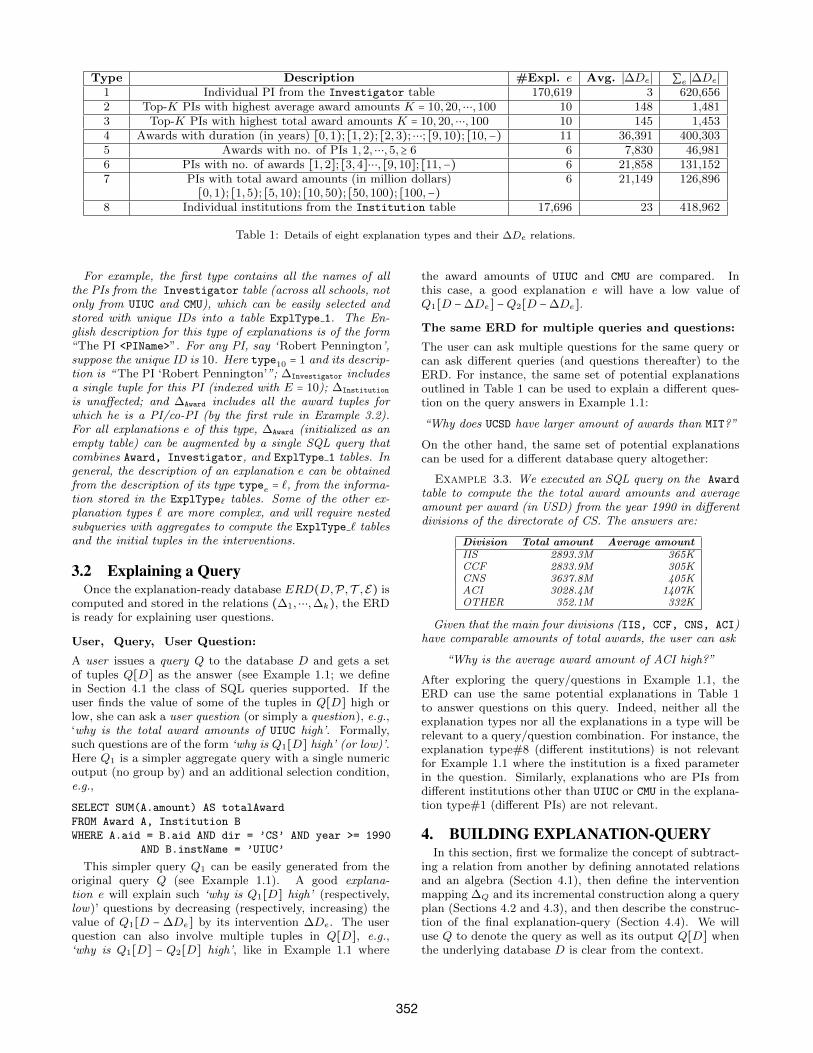
Type Description #Expl. e Avg. ∣∆De∣ ∑e ∣∆De∣
1 Individual PI from the Investigator table 170,619 3 620,6562 Top-K PIs with highest average award amounts K = 10,20,⋯,100 10 148 1,4813 Top-K PIs with highest total award amounts K = 10,20,⋯,100 10 145 1,4534 Awards with duration (in years) [0,1); [1,2); [2,3);⋯; [9,10); [10,−) 11 36,391 400,3035 Awards with no. of PIs 1,2,⋯,5,≥ 6 6 7,830 46,9816 PIs with no. of awards [1,2]; [3,4]⋯, [9,10]; [11,−) 6 21,858 131,1527 PIs with total award amounts (in million dollars) 6 21,149 126,896
[0,1); [1,5); [5,10); [10,50); [50,100); [100,−)8 Individual institutions from the Institution table 17,696 23 418,962
Table 1: Details of eight explanation types and their ∆De relations.
For example, the first type contains all the names of allthe PIs from the Investigator table (across all schools, notonly from UIUC and CMU), which can be easily selected andstored with unique IDs into a table ExplType 1. The En-glish description for this type of explanations is of the form“The PI <PIName>”. For any PI, say ‘Robert Pennington’,suppose the unique ID is 10. Here type10 = 1 and its descrip-tion is “ The PI ‘Robert Pennington’”; ∆Investigator includesa single tuple for this PI (indexed with E = 10); ∆Institution
is unaffected; and ∆Award includes all the award tuples forwhich he is a PI/co-PI (by the first rule in Example 3.2).For all explanations e of this type, ∆Award (initialized as anempty table) can be augmented by a single SQL query thatcombines Award, Investigator, and ExplType 1 tables. Ingeneral, the description of an explanation e can be obtainedfrom the description of its type typee = `, from the informa-tion stored in the ExplType` tables. Some of the other ex-planation types ` are more complex, and will require nestedsubqueries with aggregates to compute the ExplType ` tablesand the initial tuples in the interventions.
3.2 Explaining a QueryOnce the explanation-ready database ERD(D,P,T ,E) is
computed and stored in the relations (∆1,⋯,∆k), the ERDis ready for explaining user questions.
User, Query, User Question:
A user issues a query Q to the database D and gets a setof tuples Q[D] as the answer (see Example 1.1; we definein Section 4.1 the class of SQL queries supported. If theuser finds the value of some of the tuples in Q[D] high orlow, she can ask a user question (or simply a question), e.g.,‘why is the total award amounts of UIUC high’. Formally,such questions are of the form ‘why is Q1[D] high’ (or low)’.Here Q1 is a simpler aggregate query with a single numericoutput (no group by) and an additional selection condition,e.g.,
SELECT SUM(A.amount) AS totalAward
FROM Award A, Institution B
WHERE A.aid = B.aid AND dir = ’CS’ AND year >= 1990
AND B.instName = ’UIUC’
This simpler query Q1 can be easily generated from theoriginal query Q (see Example 1.1). A good explana-tion e will explain such ‘why is Q1[D] high’ (respectively,low)’ questions by decreasing (respectively, increasing) thevalue of Q1[D − ∆De] by its intervention ∆De. The userquestion can also involve multiple tuples in Q[D], e.g.,‘why is Q1[D] − Q2[D] high’, like in Example 1.1 where
the award amounts of UIUC and CMU are compared. Inthis case, a good explanation e will have a low value ofQ1[D −∆De] −Q2[D −∆De].
The same ERD for multiple queries and questions:
The user can ask multiple questions for the same query orcan ask different queries (and questions thereafter) to theERD. For instance, the same set of potential explanationsoutlined in Table 1 can be used to explain a different ques-tion on the query answers in Example 1.1:
“Why does UCSD have larger amount of awards than MIT?”
On the other hand, the same set of potential explanationscan be used for a different database query altogether:
Example 3.3. We executed an SQL query on the Award
table to compute the the total award amounts and averageamount per award (in USD) from the year 1990 in differentdivisions of the directorate of CS. The answers are:
Division Total amount Average amountIIS 2893.3M 365KCCF 2833.9M 305KCNS 3637.8M 405KACI 3028.4M 1407KOTHER 352.1M 332K
Given that the main four divisions (IIS, CCF, CNS, ACI)have comparable amounts of total awards, the user can ask
“Why is the average award amount of ACI high?”
After exploring the query/questions in Example 1.1, theERD can use the same potential explanations in Table 1to answer questions on this query. Indeed, neither all theexplanation types nor all the explanations in a type will berelevant to a query/question combination. For instance, theexplanation type#8 (different institutions) is not relevantfor Example 1.1 where the institution is a fixed parameterin the question. Similarly, explanations who are PIs fromdifferent institutions other than UIUC or CMU in the explana-tion type#1 (different PIs) are not relevant.
4. BUILDING EXPLANATION-QUERYIn this section, first we formalize the concept of subtract-
ing a relation from another by defining annotated relationsand an algebra (Section 4.1), then define the interventionmapping ∆Q and its incremental construction along a queryplan (Sections 4.2 and 4.3), and then describe the construc-tion of the final explanation-query (Section 4.4). We willuse Q to denote the query as well as its output Q[D] whenthe underlying database D is clear from the context.
352
4.1 Annotated Relations and AlgebraIn order to formalize and compute the difference in the
answers ∆Q[D,∆D], we view the base relations as well as allintermediate and final relations as annotated relations thatconsider aggregate and non-aggregate attributes separately.Let D be the domain of all attributes in the database D; weassume that the set of reals R ⊆ D.
Definition 4.1. An annotated relation S of type [A; K]is a function S ∶ Dm
→ R`, where ∣A∣ =m and ∣K∣ = `. Here A
and K are called the standard attributes and the annotationattributes of S respectively. Further, the support of S, i.e.,the number of tuples in {t ∈ Dm
∶ S(t) ≠ 0`}, is finite.
Intuitively, A corresponds to the non-aggregate attributes,and the annotation K corresponds to one or more aggre-gates when the relation has been generated by an aggregatequery). Then S(t) denotes the values of these aggregatesfor a tuple t comprising only standard attributes. Since Sis a function, A can be considered as the key of S; so, wefollow the set semantics and do not allow duplicates in anyintermediate relation3. The base relations Si, i ∈ [1, k], areannotated relations of type [Ai;K], where for all tuples t ∈ Si,Si(t) = 1. The annotation K simply corresponds to the finitesupport of the relations and is not physically stored; thisalso holds for any non-aggregate query. Here K is called thetrivial annotation and the 1/0 annotations are treated asBoolean true/false. Otherwise, when K denotes non-trivialannotations (as the result of an aggregate query), we storeS in a standard DBMS with attributes A ∪ K.
Algebra on Annotated RelationsClass of SQL queries: We support a subclass ofSQL queries Q that extends the class of single-block“select-from-where-group by” aggregate queries consid-ered in previous work [34, 32]. In particular, we allow (i)union operations in non-aggregate queries, and (ii) multiplelevels of aggregates, but do not allow selection σ, join &, andunion ∪ operations on an aggregate sub-query. This frag-ment of SQL queries can be expressed by a query plan treewhere all σ,&,∪ operators appear below all aggregate (γ)operators in the plan4. Examples include the single-blockqueries in Examples 1.1 and 3.3, and the nested query inSection 5.2. We do not support queries with bag semanticsor non-monotone queries. The grammar for the intendedaggregate query class Qa can be defined as follows (Qa,Qna
respectively denote aggregate and non-aggregate queries):
Qna = S1 ∣ ⋯ ∣Sk ∣ σc(Qna) ∣ Qna &c Qna ∣ Qna ∪Qna (2)
Qa = γA,aggr1(g1(B1)),⋯,aggrs(gs(Bs))(Qna ∣ Qa) (3)
However, the queries Qna,Qa in the above grammar corre-spond to annotated relations both as the inputs and outputs.In particular, S1,⋯, Sk are the annotated base relations inD. For this class of queries, the inputs to the non-aggregateoperators are annotated relation(s) with trivial annotationK. Therefore, the predicate c for σ and & is a predicate onthe standard attributes. Due to space constraints, we onlygive the semantic of the aggregate operator γ (the rest canbe found in the full version [4]).
Semantic of the γ operator: Let Q =
γA,aggr1(g1(B1)),⋯,aggrs(gs(Bs))Q′, where Q′ is of type
3If base relations have duplicates, the tuples can be madeunique by considering an additional id column.4This particular subclass is considered for technical reasonsas mentioned later in the paper (e.g., see Section 4.3.1).
[A′; K′], ∣A′∣ = m, ∣K′∣ = `, and each Bi ⊆ A′ ∪ K′. ThenQ is of type [A; K], where ∣K∣ = s and K stores the aggre-gates: aggr1(g1(B1)),⋯, aggrs(gs(Bs)). ∀t ∈ Dm, the j-thcomponent of Q(t), j ∈ [1, s], is:
aggrj t′∈Dm ∶t′.A′=t (gj(t′.Bj) × I[Q′(t′) ≠ 0`
])
where I[Q′(t′) ≠ 0`
] is the indicator function denot-ing whether the tuple t′ has a non-zero annotation andtherefore can possibly contribute to the aggregate. Here,aggri ∈ {sum, count, avg,min,max, count distinct} and giis a scalar function which can be a constant, an attribute,or a numeric function involving +,−,×, min,max, or anyother function supported by SQL.
Example 4.2. (1) In Q = γA,count(∗) = γA,sum(1), theaggregate function is aggr = sum; the scalar function isg(x) = 1. (2) In Q = γA,sum(B1×B2)
, aggr = sumand g(x, y) = x × y, which operates on the attributes B =
⟨B1, B2⟩. (3) In Q = γA,sum(min(B1,B2)), aggr = sum,
and g(x, y) = min(x, y). (4) In Q = γA,min(min(B1,B2)),
aggr =min, g(x, y) = min(x, y).
The semantics of the aggregate function and the scalar func-tion are different even if they use the same function like min;the scalar function applies to different attributes of the sametuple, whereas the aggregate function applies to all the tu-ples in a group with the same value of the attributes A.
From this point on, we assume that the aggregate func-tion is sum; the other operators count, avg,min /max andcount distinct can be simulated using sum (see [4]). How-ever, if min /max /count distinct/avg operators appear in anintermediate step in the query plan (which is less common inpractice), Q[D−∆D] needs to be computed from Q[D] and∆Q[D,∆D] before proceeding further; see Section 6. Sinceannotated relations require set semantic, we do not includethe projection operator π in the grammar. A projection onto a set (e.g., select distinct A, B, C from ...) can be cap-tured using the aggregate operation Q = γA,B,CQ
′, whereno aggregate value is computed for each group. The projec-tion with duplicates, which is allowed in standard databasesystems, is not allowed in our framework.
4.2 Intervention MappingIn this section we formalize the concepts described in
Example 3.1 and define the desired ∆Q query for a givenquery Q. Similar to the inputs and outputs of query Q,∆Q = ∆Q[D,∆D] will also be interpreted as an annotatedrelation, called the intervention mapping of Q.
4.2.1 Addition/Subtraction on Annotated RelationsTwo annotated relations S and S′ must have the same
type to be compatible for addition or subtraction.
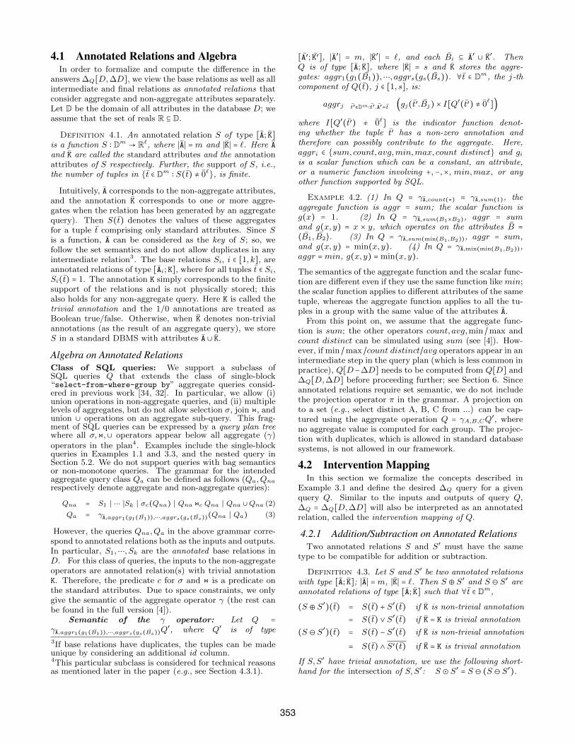
Definition 4.3. Let S and S′ be two annotated relationswith type [A; K]; ∣A∣ =m, ∣K∣ = `. Then S ⊕ S′ and S ⊖ S′ areannotated relations of type [A; K] such that ∀t ∈ Dm,
(S ⊕ S′)(t) = S(t) + S′(t) if K is non-trivial annotation
= S(t) ∨ S′(t) if K = K is trivial annotation
(S ⊖ S′)(t) = S(t) − S′(t) if K is non-trivial annotation
= S(t) ∧ S′(t) if K = K is trivial annotation
If S,S′ have trivial annotation, we use the following short-hand for the intersection of S,S′: S ⊙ S′ = S ⊖ (S ⊖ S′).
353
For relations with trivial annotations, ⊕,⊖,⊙ can be im-plemented by SQL union, minus/except, intersect respec-tively. For non-trivial annotations, a tuple present in ei-ther of S,S′ should be present in the output (even if it doesnot appear in one of the relations). Therefore, to implement⊕,⊖, we run an SQL query that performs a full outer join onthe tables S, S′ on S.A = S′.A, and computes the aggregateisnull(S.α,0) ± isnull(S′.α,0) as α for each α ∈ K. Herethe function isnull(A,0) returns 0 if A = null (when it isnot present in one of the tables), otherwise returns A.
Remark. We are referring to two join operators. Thealgebra on annotated relations includes a join operation asdefined in equation (2) to capture the standard join opera-tion supported in relational algebra or SQL. However, the ⊕and ⊖ operators described above will also require the stan-dard join (outer-join) operation in SQL when they are im-plemented. In other words, we first interpret extended rela-tional algebra operators as operators on annotated relationsin equations (2) and (3). Then to implement these operatorsin a DBMS, we translate them back to SQL queries.
4.2.2 Intervention Mapping on Base RelationsRecall that the type of annotated base relation Si is [Ai;K],
and E denotes the integer index of possible explanations.Suppose ∣Ai∣ =mi; ∣K∣ = ∣E∣ = 1.
Definition 4.4. The intervention mappings of base rela-tions, ∆i ∶ D1+mi → R for i ∈ [1, k], are annotated relationsof type [{E} ∪ Ai;K] such that K is the trivial annotation,and ∀E = e, ∀t ∈ Dmi , ∆i(⟨e, t⟩)⇒ Si(t), i.e., if the LHS is1, the RHS must also be 1.
The above condition ensures that if a tuple t ∈ Dm is deletedfrom Si for an explanation E = e, then t must exist in Si.Note that ∆i ∶ D1+mi → R is equivalent to ∆i ∶ D → [Dmi →
R]. By selecting tuples from ∆i where E = e, and discardingthe attributes E, we get another annotated relation (all thevalues of Ai are unique), which we denote by ∆i,e. Hencefor an explanation E = e, the intervention of e is given by∆De = (∆1,e,⋯,∆k,e). Further, for each explanation E = e,
the intervened relation Si due to e is precisely captured bythe annotated relation of type [Ai;K]: Si = Si ⊖ ∆i,e (seeFigure 1).
4.2.3 Intervention Mapping of a QueryNext, we generalize Definition 4.4 and define ∆Q for any
query Q that is defined through the algebra in (2) and (3).
Definition 4.5. Let D be a database comprising anno-tated relations Si of type [Ai;K], i ∈ [1, k]. Let Q be a querythat takes D as input and produces an annotated relationQ[D] of type [AQ; KQ] as output; ∣AQ∣ = m and ∣KQ∣ = `.Let E be the index of explanations and ∆i be the interventionmapping of Si, i ∈ [1, k]. Let D ⊖∆De denote the databasecomprising annotated relations S1 ⊖∆1,e,⋯, Sk ⊖∆k,e.
Then, the intervention-mapping of Q, denoted by ∆Q ∶
D1+m→ R`, equivalently ∆Q ∶ D → [Dm
→ R`], is an anno-
tated relation of type [{E}∪AQ; KQ] such that for all E = e,
Q[D] ⊖ ∆Q,e[D,∆D] = Q[D ⊖∆De] (4)
where ∆Q,e is the restriction of ∆Q to E = e that selectstuples with E = e from ∆Q and discards E.
4.3 Computing Intervention MappingNow we describe how ∆Q can be computed incrementally
along any given logical query plan tree assuming ∆i for i ∈[1, k] have been precomputed and stored. For a tuple t,an attribute a, and a vector of attributes b, t.a denotes thevalue of attribute a in t and t.b denotes the vector of thevalues of the attributes b in t.
4.3.1 For Non-Aggregate OperatorsThe rules for each non-aggregate operator in the grammar
(2) are given below (here all the input and output annotatedrelations have trivial annotations). These rules are similarto the update rules in the IVM literature [12, 18], althoughthey take into account updates for all explanations e simul-taneously. The correctness of these rules follows by induc-tion (proofs and illustrating examples appear in [4]). HereER is a relation with attribute E that contains all possiblevalues of explanation index E = e.
Base case: If Q = Si, i ∈ [1, k], return ∆Q = ∆i.Selection: If Q = σc(Q
′), return ∆Q = σc(∆Q′).
Join: If Q = Q1 &c Q2, return ∆Q = [(Q1 &c
∆Q2)⊕ (∆Q1 &c Q2)].Union: If Q = Q1 ∪ Q2, return ∆Q = [(∆Q1 ⊖ (ER ×
Q2))⊕ (∆Q2 ⊖ (ER ×Q1))]⊕ (∆Q1 ⊙∆Q2)
Remark. The proof of the rule for σc depends on theequality that σc(S ⊖ S
′) = σcS ⊖ σcS
′. However, this equal-ity does not hold if the predicate c includes annotation at-tributes K. For instance, suppose S and S′ have a single tu-ple each: ⟨t,5⟩ and ⟨t,4⟩ and the condition c checks whetherthe annotation is ≥ 2. Then, in σc(S ⊖ S
′), tuple t does not
exist, whereas the tuple t has annotation 1 in σcS ⊖ σcS′.
Therefore, we needed the restriction that c is only definedon A, which can be relaxed as discussed in Section 6.
4.3.2 For Scalar FunctionsWe define intervention mapping ∆g of a scalar function g
which measures the change in the value of g when its inputsare changed, and allows us to do further optimizations inthe incremental process of constructing ∆Q:
(∆g)(x,∆x) = g(x) − g(x −∆x) (5)
If ∆x = 0, x is unchanged, and ∆g = 0. For example,if g(x) = a constant, then ∆g = 0; if g(x) = x, ∆g = x,etc. For some functions, no simplifications are possible, e.g.,∆g = min(x, y)−min(x−∆x, y−∆y) if g(x, y) = min(x, y).
Remark. The scalar functions are applied on standardor annotation attributes. However, ∆x can be non-zero onlyif x is an annotation attribute, e.g., if a tuple r appears withannotation 7 in Q and as 3 in ∆Q,e for some E = e, thenits annotation in Q ⊖∆Q,e will be 7 - 3 = 4. On the otherhand, the standard attributes are treated as constants in thescalar functions g, as they either entirely exist in Q⊖∆Q,e
or are entirely omitted. We will see examples illustratingthis distinction in the next subsection.
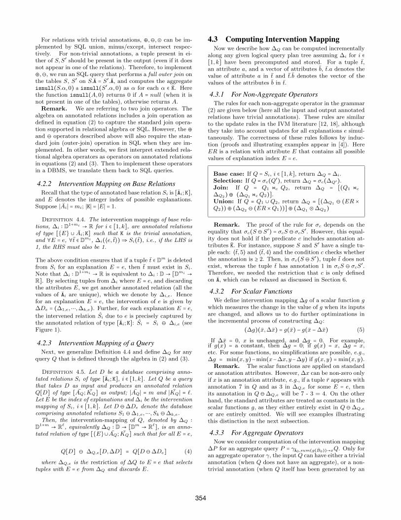
4.3.3 For Aggregate OperatorsNow we consider computation of the intervention mapping
∆P for an aggregate query P = γA0,sum(g(B0))→xQ. Only foran aggregate operator γ, the inputQ can have either a trivialannotation (when Q does not have an aggregate), or a non-trivial annotation (when Q itself has been generated by an
354
aggregate query). In this section we give a simple algorithmto compute ∆P that takes care of both these cases.
The input Q of P is of type [A, K], A0 ⊆ A, g is a scalarfunction, and B0 = B0A ∪ B0K where B0A ⊆ A and B0K ⊆ K.Clearly, P is of type [A0, x]. Without loss of generality, weconsider only one aggregate output g. By definition of ∆Pin equation (4), for any E = e,
P [D]⊖∆P,e[D,∆D] = P [D ⊖∆De]
Fix an e and consider a tuple t ∈ D` where ∣A0∣ = `. Next wecompute ∆P,e(t), i.e., the change in the annotation for t.
For simplicity, we denote the annotation of t in P [D],P [D ⊖ ∆De], and ∆P,e[D,∆D] as PD(t), PD−∆D(t), and∆PD,∆D(t) respectively (similarly for Q,∆Q etc.). Further,we denote the indicator function to check if the annotationof a tuple is non-zero, I[Q(t) ≠ 0] as bQ(t). Recall thedefinition of ∆g (5). Since PD(t)−∆PD,∆D(t) = PD−∆D(t),
∆PD,∆D(t) = PD(t) − PD−∆D(t)
= ∑r ∶ r.A0=t
g(⟨r.B0A,QD(r).B0K⟩) × bQD(r)
− g(⟨r.B0A,QD−∆D(r).B0K⟩) × bQD−∆D(r)
= ∑r∶r.A0=t
g(⟨r.B0A,QD(r).B0K⟩) × bQD(r)
− g(⟨r.B0A,QD(r).B0K⟩) × bQD−∆D(r) + bQD−∆D(r)×
∆g(⟨r.B0A,QD(r).B0K⟩, ⟨r.B0A,∆QD(r).B0K⟩)
Interestingly, this complex expression can be simplified andefficiently implemented using the properties of a monotonequery. Due to space constraints, here we give the algorithm;the analysis can be found in the full version [4].
Perform a semi-join ∆Q ⋉∆Q.A=Q.A Q, where A is the setof all standard attributes of Q, and compute a newattribute y as follows: if Q.K = ∆Q.K then
/* (Case 1): This includes the case when K is thetrivial annotation */ ;
y = g(⟨Q.B0A,Q. ¯B0K⟩)
endelse
/* (Case 2) */ ;
y = ∆g(⟨Q.B0A,Q.B0K⟩, ⟨Q.B0A,∆Q.B0K⟩)
end
Perform Group By on B0A and store sum(y) as x.Algorithm 1: Generic algorithm for computing ∆P from∆Q, where P = γA0,sum(g(B0))→xQ
There is a subtle difference between how standard at-tributes and annotation attributes are treated in the abovealgorithm, which we illustrate with the examples below. Inthe first example, there are no non-trivial annotation at-tributes.
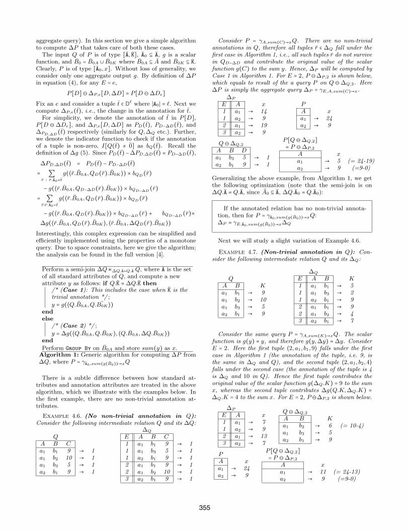
Example 4.6. (No non-trivial annotation in Q):Consider the following intermediate relation Q and its ∆Q:
QA B Ca1 b1 9 → 1a1 b2 10 → 1a1 b3 5 → 1a2 b1 9 → 1
∆Q
E A B C1 a1 b1 9 → 11 a1 b3 5 → 11 a2 b1 9 → 12 a1 b1 9 → 12 a1 b2 10 → 13 a2 b1 9 → 1
Consider P = γA,sum(C)→xQ. There are no non-trivialannotations in Q, therefore all tuples r ∈ ∆Q fall under thefirst case in Algorithm 1, i.e., all such tuples r do not survivein QD−∆D and contribute the original value of the scalarfunction g(C) to the sum y. Hence, ∆P will be computed byCase 1 in Algorithm 1. For E = 2, P ⊖∆P,2 is shown below,which equals to result of the a query P on Q ⊖∆Q,2. Here∆P is simply the aggregate query ∆P = γE,A,sum(C)→x.
∆P
E A x1 a1 → 141 a2 → 92 a1 → 193 a2 → 9
PA xa1 → 24a2 → 9
Q⊖∆Q,2
A B Da1 b3 5 → 1a2 b1 9 → 1
P [Q⊖∆Q,2]
= P ⊖∆P,2
A xa1 → 5 (= 24-19)a2 → 9 (=9-0)
Generalizing the above example, from Algorithm 1, we getthe following optimization (note that the semi-join is on∆Q.A = Q.A, since A0 ⊆ A, ∆Q.A0 = Q.A0):
If the annotated relation has no non-trivial annota-tion, then for P = γA0,sum(g(B0))→xQ:∆P = γE,A0,sum(g(B0))→x∆Q
Next we will study a slight variation of Example 4.6.
Example 4.7. (Non-trivial annotation in Q): Con-sider the following intermediate relation Q and its ∆Q:
QA B Ka1 b1 → 9a1 b2 → 10a1 b3 → 5a2 b1 → 9
∆Q
E A B K1 a1 b1 → 51 a1 b3 → 21 a2 b1 → 92 a1 b1 → 92 a1 b2 → 43 a2 b1 → 7
Consider the same query P = γA,sum(K)→xQ. The scalarfunction is g(y) = y, and therefore g(y,∆y) = ∆y. ConsiderE = 2. Here the first tuple ⟨2, a1, b1,9⟩ falls under the firstcase in Algorithm 1 (the annotation of the tuple, i.e. 9, isthe same in ∆Q and Q), and the second tuple ⟨2, a1, b2,4⟩falls under the second case (the annotation of the tuple is 4is ∆Q and 10 in Q). Hence the first tuple contributes theoriginal value of the scalar function g(∆Q.K) = 9 to the sumx, whereas the second tuple contributes ∆g(Q.K,∆Q.K) =
∆Q.K = 4 to the sum x. For E = 2, P ⊖∆P,2 is shown below.
∆P
E A x1 a1 → 71 a2 → 92 a1 → 133 a2 → 7
Q⊖∆Q,2
A B Ka1 b2 → 6 (= 10-4)a1 b3 → 5a2 b1 → 9
PA xa1 → 24a2 → 9
P [Q⊖∆Q,2]
= P ⊖∆P,2
A xa1 → 11 (= 24-13)a2 → 9 (=9-0)
355
Interestingly, similar to Example 4.6, ∆P in Example 4.7also can be computed as ∆P = γE,A,sum(K)→x∆Q. How-ever, this follows due to a completely different argument.The most common scalar function is g(x) = x, i.e., thex = sum(C) for an attribute C. If C ∈ K is an annota-tion attribute, then in case 1, g = Q.C = ∆Q.C, and incase 2, ∆g = g(Q.C) − g(Q.C − ∆Q.C) = ∆Q.C. Note that∆g(x,∆x) = ∆x (i.e., the additive nature of sum(C)) isimportant here – for other scalar functions g such that ∆ginvolves both x,∆x (e.g., g(x) = x2,min(x) etc.), the semi-join of ∆Q with Q will be necessary. This gives the secondoptimization rule:
For P = γA0,sum(C)→xQ, where C ∈ K is an annotationattribute (or is a constant), ∆P = γE,A0,sum(C)→x∆Q
A special case of the above rule is when C = 1 or otherreal constants, which can be treated as trivial annotations.Therefore, the above optimization can be applied for countqueries like P = γA0,sum(1)→xQ.
Remark. The above optimization rule does not hold ifC ∈ A is a standard attribute. In case 1, similar to the above,g = Q.C = ∆Q.C. However, to check if the tuple falls undercase 1, the semi-join is needed. This is due to the fact thatin case 2, ∆g = g(Q.C) − g(Q.C) = 0 and not ∆Q.C, i.e., ifa tuple r survives in Q−∆Q, it contributes Q.C entirely tothe sum as C is a standard attribute and not an annotationattribute.
4.4 Explanation-Query fromIntervention Mapping
To compute Q[D ⊖ ∆De], we do not need to computeQ[D] ⊖ ∆Q,e[D,∆D] for each e. Instead, a left outer-joinis performed between the original query answer Q[D] and∆Q[D,∆D] on equal values of standard attributes AQ, agroup by is performed on {E}∪AQ, and the updated annota-tions are computed by subtraction or set difference of ∆Q.Kfrom Q.K for each such group (that will have the same valuee of E) for non-trivial and trivial annotations respectively;only the non-zero results are returned. However, sometimesthe difference of the original and the new query captured bythe ∆Q[D,∆D] relation will suffice to rank the explanations(e.g., when the aggregate function is additive), and then thisjoin at the end can be avoided. The explanation-query (allsteps of ∆Q and the final outer-join with Q if needed) is sentto the DBMS as a single query to utilize the optimizationsby the DBMS. If the user question involves multiples queries,then explanation query is constructed for all of them, andthe answers are combined for the final ranking of explana-tions by a top-k query (an example is in Section 5.2).
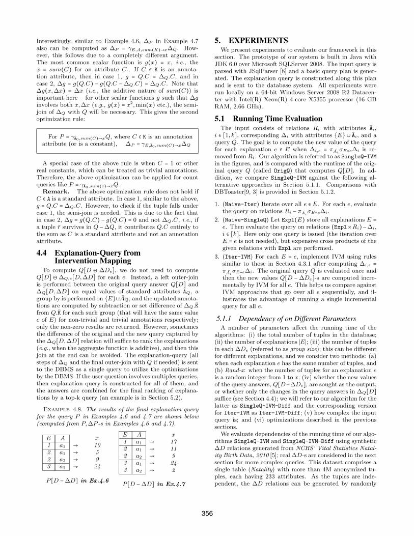
Example 4.8. The results of the final explanation queryfor the query P in Examples 4.6 and 4.7 are shown below(computed from P,∆P -s in Examples 4.6 and 4.7).
E A x1 a1 → 102 a1 → 52 a2 → 93 a1 → 24
P [D −∆D] in Ex.4.6
E A x1 a1 → 172 a1 → 112 a2 → 93 a1 → 243 a2 → 2
P [D −∆D] in Ex.4.7
5. EXPERIMENTSWe present experiments to evaluate our framework in this
section. The prototype of our system is built in Java withJDK 6.0 over Microsoft SQLServer 2008. The input query isparsed with JSqlParser [8] and a basic query plan is gener-ated. The explanation query is constructed along this planand is sent to the database system. All experiments wererun locally on a 64-bit Windows Server 2008 R2 Datacen-ter with Intel(R) Xeon(R) 4-core X5355 processor (16 GBRAM, 2.66 GHz).
5.1 Running Time EvaluationThe input consists of relations Ri with attributes Ai,
i ∈ [1, k], corresponding ∆i with attributes {E} ∪ Ai, and aquery Q. The goal is to compute the new value of the queryfor each explanation e ∈ E when ∆i,e = πAi
σE=e∆i is re-moved from Ri. Our algorithm is referred to as SingleQ-IVMin the figures, and is compared with the runtime of the orig-inal query Q (called OrigQ) that computes Q[D]. In ad-dition, we compare SingleQ-IVM against the following al-ternative approaches in Section 5.1.1. Comparisons withDBToaster[9, 3] is provided in Section 5.1.2.
1. (Naive-Iter) Iterate over all e ∈ E. For each e, evaluatethe query on relations Ri − πAi
σE=e∆i.
2. (Naive-SingleQ) Let Expl(E) store all explanations E =
e. Then evaluate the query on relations (Expl×Ri)−∆i,i ∈ [k]. Here only one query is issued (the iteration overE = e is not needed), but expensive cross products of thegiven relations with Expl are performed.
3. (Iter-IVM) For each E = e, implement IVM using rulessimilar to those in Section 4.3.1 after computing ∆i,e =
πAiσE=e∆i. The original query Q is evaluated once and
then the new values Q[D − ∆De]-s are computed incre-mentally by IVM for all e. This helps us compare againstIVM approaches that go over all e sequentially, and il-lustrates the advantage of running a single incrementalquery for all e.
5.1.1 Dependency of on Different ParametersA number of parameters affect the running time of the
algorithms: (i) the total number of tuples in the database;(ii) the number of explanations ∣E∣; (iii) the number of tuplesin each ∆De (referred to as group size); this can be differentfor different explanations, and we consider two methods: (a)when each explanation e has the same number of tuples, and(b) Rand-x: when the number of tuples for an explanation eis a random integer from 1 to x; (iv) whether the new valuesof the query answers, Q[D−∆De], are sought as the output,or whether only the changes in the query answers in ∆Q[D]
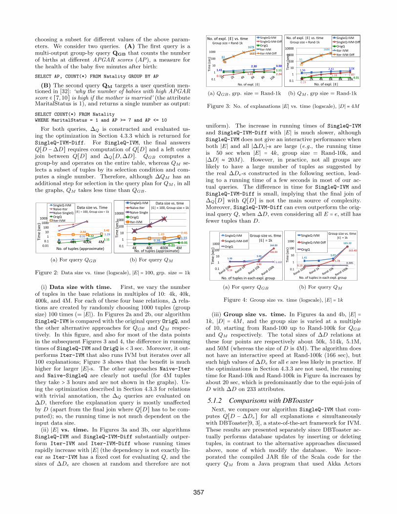
suffice (see Section 4.4); we will refer to our algorithm for thelatter as SingleQ-IVM-Diff and the corresponding versionfor Iter-IVM as Iter-IVM-Diff; (v) how complex the inputquery is; and (vi) optimizations described in the previoussections.
We evaluate dependencies of the running time of our algo-rithms SingleQ-IVM and SingleQ-IVM-Diff using synthetic∆D relations generated from NCHS’ Vital Statistics Natal-ity Birth Data, 2010 [5]; real ∆D-s are considered in the nextsection for more complex queries. This dataset comprises asingle table (Natality) with more than 4M anonymized tu-ples, each having 233 attributes. As the tuples are inde-pendent, the ∆D relations can be generated by randomly
356
choosing a subset for different values of the above param-eters. We consider two queries. (A) The first query is amulti-output group-by query QGB that counts the numberof births at different APGAR scores (AP ), a measure forthe health of the baby five minutes after birth:
SELECT AP, COUNT(*) FROM Natality GROUP BY AP
(B) The second query QM targets a user question men-tioned in [32]: ‘why the number of babies with high APGARscore ∈ [7,10] is high if the mother is married’ (the attributeMaritalStatus is 1), and returns a single number as output:
SELECT COUNT(*) FROM NatalityWHERE MaritalStatus = 1 and AP >= 7 and AP <= 10
For both queries, ∆Q is constructed and evaluated us-ing the optimization in Section 4.3.3 which is returned forSingleQ-IVM-Diff. For SingleQ-IVM, the final answersQ[D −∆D] requires computation of Q[D] and a left outerjoin between Q[D] and ∆Q[D,∆D]. QGB computes agroup-by and operates on the entire table, whereas QM se-lects a subset of tuples by its selection condition and com-putes a single number. Therefore, although ∆QM has anadditional step for selection in the query plan for QM , in allthe graphs, QM takes less time than QGB .
2.50 3.42
0.12 1.11
0.31 1.29
0.01 0.1 1 10
100 1000 10000
4k 40k 400k 4M
Time (sec)
No. of tuples (approximate)
Data size vs. Time |E| = 100, Group size = 1k
SingleQ-‐IVM Naïve-‐Iter Naïve-‐SingleQ OrigQ Iter-‐IVM
(a) For query QGB
1.49 2.46
0.38 1.55
0.21 0.31
0.1
1
10
100
1000
10000
4K 40K 400K 4M
Time (sec)
No. of tuples (approximate)
Data size vs. =me |E| = 100, Group size = 1k
SingleQ-‐IVM Naïve-‐Iter Naïve-‐Single OrigQ Iter-‐IVM
(b) For query QM
Figure 2: Data size vs. time (logscale), ∣E∣ = 100, grp. size = 1k
(i) Data size with time. First, we vary the numberof tuples in the base relations in multiples of 10: 4k, 40k,400k, and 4M. For each of these four base relations, ∆ rela-tions are created by randomly choosing 1000 tuples (groupsize) 100 times (= ∣E∣). In Figures 2a and 2b, our algorithmSingleQ-IVM is compared with the original query OrigQ, andthe other alternative approaches for QGB and QM respec-tively. In this figure, and also for most of the data pointsin the subsequent Figures 3 and 4, the difference in runningtimes of SingleQ-IVM and OrigQ is < 3 sec. Moreover, it out-performs Iter-IVM that also runs IVM but iterates over all100 explanations; Figure 3 shows that the benefit is muchhigher for larger ∣E∣-s. The other approaches Naive-Iter
and Naive-SingleQ are clearly not useful (for 4M tuplesthey take > 3 hours and are not shown in the graphs). Us-ing the optimization described in Section 4.3.3 for relationswith trivial annotation, the ∆Q queries are evaluated on∆D, therefore the explanation query is mostly unaffectedby D (apart from the final join where Q[D] has to be com-puted); so, the running time is not much dependent on theinput data size.
(ii) ∣E∣ vs. time. In Figures 3a and 3b, our algorithmsSingleQ-IVM and SingleQ-IVM-Diff substantially outper-form Iter-IVM and Iter-IVM-Diff whose running timesrapidly increase with ∣E∣ (the dependency is not exactly lin-ear as Iter-IVM has a fixed cost for evaluating Q, and thesizes of ∆De are chosen at random and therefore are not
1.41 2.30 3.50
0.31 1.22 2.24
61
1678
1.11
48
1637
0.1
1
10
100
1000
1k 2k 4k 6k 8k 10k
Time (sec)
No. of expl. |E|
No. of expl. |E| vs. ;me Group size = Rand-‐1k
SingleQ-‐IVM SingleQ-‐IVM-‐Diff OrigQ Iter-‐IVM Iter-‐IVM-‐Diff
(a) QGB , grp. size = Rand-1k
55
1686
51
0.31
1.56 2.41 3.04
0.19
1.18 1.85
0.1
1
10
100
1000
10000
1k 2k 4k 6k 8k 10k
Time (sec)
No. of expl. |E|
No. of expl. |E| vs. >me Group size = Rand-‐1k
SingleQ-‐IVM SingleQ-‐IVM-‐Diff OrigQ Iter-‐IVM Iter-‐IVM-‐Diff
(b) QM , grp size = Rand-1k
Figure 3: No. of explanations ∣E∣ vs. time (logscale), ∣D∣ = 4M
uniform). The increase in running times of SingleQ-IVM
and SingleQ-IVM-Diff with ∣E∣ is much slower, althoughSingleQ-IVM does not give an interactive performance whenboth ∣E∣ and all ∣∆De∣-s are large (e.g., the running timeis 50 sec when ∣E∣ = 4k, group size = Rand-10k, and∣∆D∣ ≈ 20M). However, in practice, not all groups arelikely to have a large number of tuples as suggested bythe real ∆De-s constructed in the following section, lead-ing to a running time of a few seconds in most of our ac-tual queries. The difference in time for SingleQ-IVM andSingleQ-IVM-Diff is small, implying that the final join of∆Q[D] with Q[D] is not the main source of complexity.Moreover, SingleQ-IVM-Diff can even outperform the orig-inal query Q, when ∆D, even considering all E = e, still hasfewer tuples than D.
0.19
1.80
166.00
1.30 3.00
164.00
1.112
0.1
1
10
100
1000
Rand-‐1
00
Rand-‐1
k
Rand-‐1
0k
Rand-‐1
00k
Time (sec)
No. of tuples in each expl. group
Group size vs. Ame |E| = 1k
SingleQ-‐IVM
SingleQ-‐IVM-‐Diff
OrigQ
(a) For query QGB
0.19 1.78
163.40
1.41 3.07
165.32
0.305
0.1
1
10
100
1000
Rand-‐1
00
Rand-‐1
k
Rand-‐1
0k
Rand-‐1
00k
Time (sec)
No. of tuples in each expl. group
Group size vs. Ame |E| = 1k SingleQ-‐IVM
SingleQ-‐IVM-‐Diff
OrigQ
(b) For query QM
Figure 4: Group size vs. time (logscale), ∣E∣ = 1k
(iii) Group size vs. time. In Figures 4a and 4b, ∣E∣ =
1k, ∣D∣ = 4M , and the group size is varied at a multipleof 10, starting from Rand-100 up to Rand-100k for QGB
and QM respectively. The total sizes of ∆D relations atthese four points are respectively about 50k, 514k, 5.1M,and 50M (whereas the size of D is 4M). The algorithm doesnot have an interactive speed at Rand-100k (166 sec), butsuch high values of ∆De for all e are less likely in practice. Ifthe optimizations in Section 4.3.3 are not used, the runningtime for Rand-10k and Rand-100k in Figure 4a increases byabout 20 sec, which is predominantly due to the equi-join ofD with ∆D on 233 attributes.
5.1.2 Comparisons with DBToasterNext, we compare our algorithm SingleQ-IVM that com-
putes Q[D − ∆De] for all explanations e simultaneouslywith DBToaster[9, 3], a state-of-the-art framework for IVM.These results are presented separately since DBToaster ac-tually performs database updates by inserting or deletingtuples, in contrast to the alternative approaches discussedabove, none of which modify the database. We incor-porated the compiled JAR file of the Scala code for thequery QM from a Java program that used Akka Actors
357
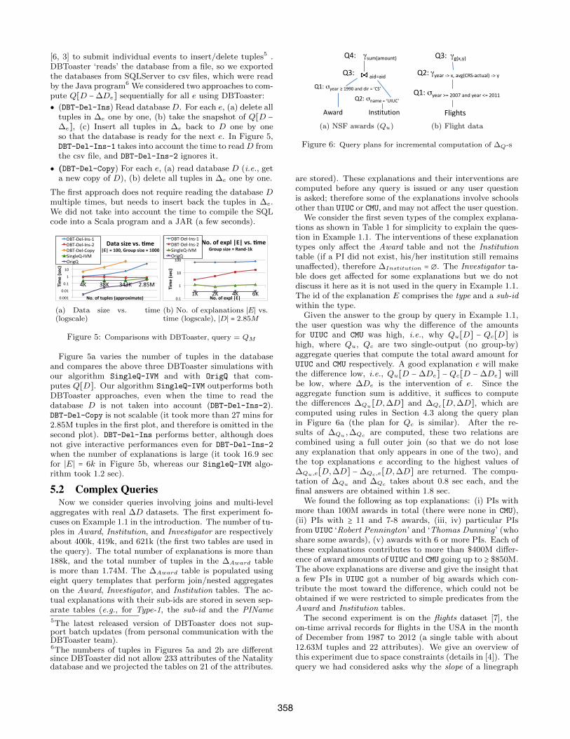
[6, 3] to submit individual events to insert/delete tuples5 .DBToaster ‘reads’ the database from a file, so we exportedthe databases from SQLServer to csv files, which were readby the Java program6 We considered two approaches to com-pute Q[D −∆De] sequentially for all e using DBToaster:
● (DBT-Del-Ins) Read database D. For each e, (a) delete alltuples in ∆e one by one, (b) take the snapshot of Q[D −
∆e], (c) Insert all tuples in ∆e back to D one by oneso that the database is ready for the next e. In Figure 5,DBT-Del-Ins-1 takes into account the time to readD fromthe csv file, and DBT-Del-Ins-2 ignores it.
● (DBT-Del-Copy) For each e, (a) read database D (i.e., geta new copy of D), (b) delete all tuples in ∆e one by one.
The first approach does not require reading the database Dmultiple times, but needs to insert back the tuples in ∆e.We did not take into account the time to compile the SQLcode into a Scala program and a JAR (a few seconds).
0.001
0.01
0.1
1
10
100
1000
4K 38K 343K 2.85M Time (sec)
No. of tuples (approximate)
Data size vs. 8me |E| = 100, Group size = 1000
DBT-‐Del-‐Ins-‐1 DBT-‐Del-‐Ins-‐2 DBT-‐Del-‐Copy SingleQ-‐IVM OrigQ
(a) Data size vs. time(logscale)
0.1
1
10
100
1K 2K 4K 6K
Time (sec)
No. of expl |E|
No. of expl |E| vs. 4me Group size = Rand-‐1k
DBT-‐Del-‐Ins-‐1 DBT-‐Del-‐Ins-‐2 SingleQ-‐IVM OrigQ
(b) No. of explanations ∣E∣ vs.time (logscale), ∣D∣ = 2.85M
Figure 5: Comparisons with DBToaster, query = QM
Figure 5a varies the number of tuples in the databaseand compares the above three DBToaster simulations withour algorithm SingleQ-IVM and with OrigQ that com-putes Q[D]. Our algorithm SingleQ-IVM outperforms bothDBToaster approaches, even when the time to read thedatabase D is not taken into account (DBT-Del-Ins-2).DBT-Del-Copy is not scalable (it took more than 27 mins for2.85M tuples in the first plot, and therefore is omitted in thesecond plot). DBT-Del-Ins performs better, although doesnot give interactive performances even for DBT-Del-Ins-2
when the number of explanations is large (it took 16.9 secfor ∣E∣ = 6k in Figure 5b, whereas our SingleQ-IVM algo-rithm took 1.2 sec).
5.2 Complex QueriesNow we consider queries involving joins and multi-level
aggregates with real ∆D datasets. The first experiment fo-cuses on Example 1.1 in the introduction. The number of tu-ples in Award, Institution, and Investigator are respectivelyabout 400k, 419k, and 621k (the first two tables are used inthe query). The total number of explanations is more than188k, and the total number of tuples in the ∆Award tableis more than 1.74M. The ∆Award table is populated usingeight query templates that perform join/nested aggregateson the Award, Investigator, and Institution tables. The ac-tual explanations with their sub-ids are stored in seven sep-arate tables (e.g., for Type-1, the sub-id and the PIName5The latest released version of DBToaster does not sup-port batch updates (from personal communication with theDBToaster team).6The numbers of tuples in Figures 5a and 2b are differentsince DBToaster did not allow 233 attributes of the Natalitydatabase and we projected the tables on 21 of the attributes.
Award
Q1: σyear ≥ 1990 and dir = ‘CS’
Q3:
Q4: γsum(amount)
Institution
Q2: σname = ‘UIUC’
aid=aid
(a) NSF awards (Qu)
Flights
Q1: σyear >= 2007 and year <= 2011
Q2: γyear -‐> x, avg(CRS-‐actual) -‐> y
Q3: γg(x,y)
(b) Flight data
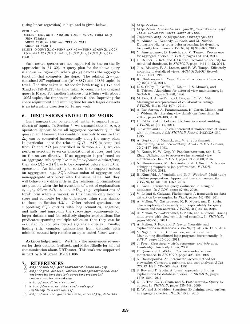
Figure 6: Query plans for incremental computation of ∆Q-s
are stored). These explanations and their interventions arecomputed before any query is issued or any user questionis asked; therefore some of the explanations involve schoolsother than UIUC or CMU, and may not affect the user question.
We consider the first seven types of the complex explana-tions as shown in Table 1 for simplicity to explain the ques-tion in Example 1.1. The interventions of these explanationtypes only affect the Award table and not the Institutiontable (if a PI did not exist, his/her institution still remainsunaffected), therefore ∆Institution = ∅. The Investigator ta-ble does get affected for some explanations but we do notdiscuss it here as it is not used in the query in Example 1.1.The id of the explanation E comprises the type and a sub-idwithin the type.
Given the answer to the group by query in Example 1.1,the user question was why the difference of the amountsfor UIUC and CMU was high, i.e., why Qu[D] − Qc[D] ishigh, where Qu, Qc are two single-output (no group-by)aggregate queries that compute the total award amount forUIUC and CMU respectively. A good explanation e will makethe difference low, i.e., Qu[D − ∆De] − Qc[D − ∆De] willbe low, where ∆De is the intervention of e. Since theaggregate function sum is additive, it suffices to computethe differences ∆Qu[D,∆D] and ∆Qc[D,∆D], which arecomputed using rules in Section 4.3 along the query planin Figure 6a (the plan for Qc is similar). After the re-sults of ∆Qu ,∆Qc are computed, these two relations arecombined using a full outer join (so that we do not loseany explanation that only appears in one of the two), andthe top explanations e according to the highest values of∆Qu,e[D,∆D] − ∆Qc,e[D,∆D] are returned. The compu-tation of ∆Qu and ∆Qc takes about 0.8 sec each, and thefinal answers are obtained within 1.8 sec.
We found the following as top explanations: (i) PIs withmore than 100M awards in total (there were none in CMU),(ii) PIs with ≥ 11 and 7-8 awards, (iii, iv) particular PIsfrom UIUC ‘Robert Pennington’ and ‘Thomas Dunning ’ (whoshare some awards), (v) awards with 6 or more PIs. Each ofthese explanations contributes to more than $400M differ-ence of award amounts of UIUC and CMU going up to ≥ $850M.The above explanations are diverse and give the insight thata few PIs in UIUC got a number of big awards which con-tribute the most toward the difference, which could not beobtained if we were restricted to simple predicates from theAward and Institution tables.
The second experiment is on the flights dataset [7], theon-time arrival records for flights in the USA in the monthof December from 1987 to 2012 (a single table with about12.63M tuples and 22 attributes). We give an overview ofthis experiment due to space constraints (details in [4]). Thequery we had considered asks why the slope of a linegraph
358
(using linear regression) is high and is given below:
WITH R AS(SELECT YEAR as x, AVG(CRS_TIME - ACTUAL_TIME) as yFROM FlightsWHERE YEAR >= 2007 and YEAR <= 2011GROUP BY YEAR )
SELECT ((COUNT(R.x)*SUM(R.x*R.y))-(SUM(R.x)*SUM(R.y)))/((count(R.X)*(SUM(R.x*R.x))-(SUM(R.x))*(SUM(R.x))))
FROM R
Such nested queries are not supported by the on-the-flyapproaches in [34, 32]. A query plan for the above queryis shown in Figure 6b, where g(x,y) denotes the aggregatefunction that computes the slope. The relation ∆Flights
contained 887 explanations (∣E∣ = 887) and 138M tuples intotal. The time taken is 82 sec for both SingleQ-IVM andSingleQ-IVM-Diff; the time taken to compute the originalquery is 10 sec. For another instance of ∆Flights with about100M tuples, the time taken is about 61 sec. Improving thespace requirement and running time for such larger datasetsis an interesting direction for future work.
6. DISCUSSIONS AND FUTURE WORKOur framework can be extended further to support larger
classes of inputs. In Section 3, we assumed that all σ,&,∪operators appear below all aggregate operators γ in thequery plan. However, this condition was only to ensure that∆Q can be computed incrementally along the query plan.In particular, once the relation Q[D − ∆D] is computedfrom D and ∆D (as described in Section 4.2.3), we canperform selection (even on annotation attributes) and joinon the answer directly. If an aggregate is performed onan aggregate sub-query like min /max /count distinct/avg,then also Q[D−∆D] has to be computed before any furtheroperation. An interesting direction is to support unionson aggregates: e.g., SQL allows union of aggregate andnon-aggregate attributes with the same name, but theywill behave very differently in ∆Q relations. Optimizationsare possible when the interventions of a set of explanationse1,⋯, en follow ∆De1 ⊆ ⋯ ⊆ ∆Den (e.g., explanations oftop-k form where k varies); in this case we only need tostore and compute for the differences using rules similarto those in Section 4.3.1. Other related questions aresupporting SQL queries with bag semantics, negation,and nulls, and improving the space/time requirements forlarger datasets and for relatively simpler explanations likepredicates spanning multiple tables so that they can beevaluated for complex nested aggregate queries. Finally,finding rich, complex explanations from datasets withminimal manual help remains an open-ended future work.
Acknowledgement. We thank the anonymous review-ers for their detailed feedback, and Milos Nikolic for helpfulcommunication about DBToaster. This work was supportedin part by NSF grant IIS-0911036.
7. REFERENCES[1] http: // www. nsf. gov/ awardsearch/ download. jsp .[2] http: // grad-schools. usnews. rankingsandreviews. com/
best-graduate-schools/ top-science-schools/computer-science-rankings .
[3] http: // www. dbtoaster. org/ .[4] https: // users. cs. duke. edu/ ~ sudeepa/
ExplReady-FullVersion. pdf .[5] http: // www. cdc. gov/ nchs/ data_ access/ ftp_ data. htm .
[6] http: // akka. io .
[7] http: // www. transtats. bts. gov/ DL_ SelectFields. asp?Table_ ID= 236& DB_ Short_ Name= On-Time .
[8] Jsqlparser. http: // jsqlparser. sourceforge. net .[9] Y. Ahmad, O. Kennedy, C. Koch, and M. Nikolic.
Dbtoaster: Higher-order delta processing for dynamic,frequently fresh views. PVLDB, 5(10):968–979, 2012.
[10] Y. Amsterdamer, D. Deutch, and V. Tannen. Provenancefor aggregate queries. In PODS, pages 153–164, 2011.
[11] G. Bender, L. Kot, and J. Gehrke. Explainable security forrelational databases. In SIGMOD, pages 1411–1422, 2014.
[12] J. A. Blakeley, P.-A. Larson, and F. W. Tompa. Efficientlyupdating materialized views. ACM SIGMOD Record,15(2):61–71, 1986.
[13] R. Chirkova and J. Yang. Materialized views. Databases,4(4):295–405, 2011.
[14] L. S. Colby, T. Griffin, L. Libkin, I. S. Mumick, andH. Trickey. Algorithms for deferred view maintenance. InSIGMOD, pages 469–480, 1996.
[15] M. Das, S. Amer-Yahia, G. Das, and C. Yu. Mri:Meaningful interpretations of collaborative ratings.PVLDB, 4(11):1063–1074, 2011.
[16] A. Das Sarma, A. Parameswaran, H. Garcia-Molina, andJ. Widom. Synthesizing view definitions from data. InICDT, pages 89–103, 2010.
[17] D. Fabbri and K. LeFevre. Explanation-based auditing.PVLDB, 5(1):1–12, 2011.
[18] T. Griffin and L. Libkin. Incremental maintenance of viewswith duplicates. ACM SIGMOD Record, 24(2):328–339,1995.
[19] A. Gupta, I. S. Mumick, and V. S. Subrahmanian.Maintaining views incrementally. ACM SIGMOD Record,22(2):157–166, 1993.
[20] Y. Katsis, K. W. Ong, Y. Papakonstantinou, and K. K.Zhao. Utilizing ids to accelerate incremental viewmaintenance. In SIGMOD, pages 1985–2000, 2015.
[21] N. Khoussainova, M. Balazinska, and D. Suciu. Perfxplain:debugging mapreduce job performance. PVLDB,5(7):598–609, 2012.
[22] B. Kimelfeld, J. Vondrak, and D. P. Woodruff. Multi-tupledeletion propagation: Approximations and complexity.PVLDB, 6(13):1558–1569, 2013.
[23] C. Koch. Incremental query evaluation in a ring ofdatabases. In PODS, pages 87–98, 2010.
[24] V. Le and S. Gulwani. Flashextract: A framework for dataextraction by examples. In PLDI, pages 542–553, 2014.
[25] A. Meliou, W. Gatterbauer, K. F. Moore, and D. Suciu.The complexity of causality and responsibility for queryanswers and non-answers. PVLDB, 4(1):34–45, 2010.
[26] A. Meliou, W. Gatterbauer, S. Nath, and D. Suciu. Tracingdata errors with view-conditioned causality. In SIGMOD,pages 505–516, 2011.
[27] A. Meliou, S. Roy, and D. Suciu. Causality andexplanations in databases. PVLDB, 7(13):1715–1716, 2014.
[28] V. Nigam, L. Jia, B. Thau Loo, and A. Scedrov.Maintaining distributed logic programs incrementally. InPPDP, pages 125–136, 2011.
[29] J. Pearl. Causality: models, reasoning, and inference.Cambridge University Press, 2000.
[30] D. Quass and J. Widom. On-line warehouse viewmaintenance. In SIGMOD, pages 393–404, 1997.
[31] N. Roussopoulos. An incremental access method forviewcache: Concept, algorithms, and cost analysis. ACMTODS, 16(3):535–563, Sept. 1991.
[32] S. Roy and D. Suciu. A formal approach to findingexplanations for database queries. In SIGMOD, pages1579–1590, 2014.
[33] Q. T. Tran, C.-Y. Chan, and S. Parthasarathy. Query byoutput. In SIGMOD, pages 535–548, 2009.
[34] E. Wu and S. Madden. Scorpion: Explaining away outliersin aggregate queries. PVLDB, 6(8), 2013.
359