Inferences for Regression Chapter 27. An Example: Body Fat and Waist Size Our chapter example revolves around the relationship between % body fat and

Inferences for Regression

Chapter 27

An Example: Body Fat and Waist Size

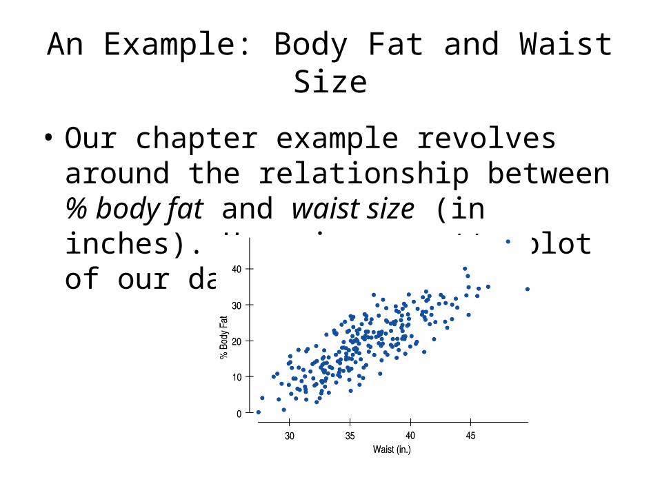
• Our chapter example revolves around the relationship between % body fat and waist size (in inches). Here is a scatterplot of our data set:

Remembering Regression

• In regression, we want to model the relationship between two quantitative variables, one the predictor and the other the response.

• To do that, we imagine an idealized regression line, which assumes that the means of the distributions of the response variable fall along the line even though individual values are scattered around it.

Remembering Regression

• Now we’d like to know what the regression model can tell us beyond the individuals in the study.

• We want to make confidence intervals and test hypotheses about the slope and intercept of the regression line.

The Population and the Sample

• When we found a confidence interval for a mean, we could imagine a single, true underlying value for the mean.

• When we tested whether two means or two proportions were equal, we imagined a true underlying difference.

• What does it mean to do inference for regression?


• We know better than to think that even if we knew every population value, the data would line up perfectly on a straight line.

• In our sample, there’s a whole distribution of %body fat for men with 38-inch waists:


• This is true at each waist size.• We could depict the distribution of %body fat

at different waist sizes like this:


• The model assumes that the means of the distributions of %body fat for each waist size fall along the line even though the individuals are scattered around it.

• The model is not a perfect description of how the variables are associated, but it may be useful.

• If we had all the values in the population, we could find the slope and intercept of the idealized regression line explicitly by using least squares.


• We write the idealized line with Greek letters and consider the coefficients to be parameters: 0 is the intercept and 1 is the slope.

• Corresponding to our fitted line of , we write

• Now, not all the individual y’s are at these means—some lie above the line and some below. Like all models, there are errors.

01 ybbx

0 1y x


• Denote the errors by . These errors are random, of course, and can be positive or negative.

• When we add error to the model, we can talk about individual y’s instead of means:

This equation is now true for each data point (since there is an to soak up the deviation) and gives a value of y for each x.

0 1y x

Assumptions and Conditions

• In Chapter 8 when we fit lines to data, we needed to check only the Straight Enough Condition.

• Now, when we want to make inferences about the coefficients of the line, we’ll have to make more assumptions (and thus check more conditions).

• We need to be careful about the order in which we check conditions. If an initial assumption is not true, it makes no sense to check the later ones.


1. Linearity Assumption:– Straight Enough Condition: Check the scatterplot

—the shape must be linear or we can’t use regression at all.


1. Linearity Assumption:– If the scatterplot is straight enough, we can go

on to some assumptions about the errors. If not, stop here, or consider re-expressing the data to make the scatterplot more nearly linear.

– Check the Quantitative Data Condition. The data must be quantitative for this to make sense.


2. Independence Assumption:– Randomization Condition: the individuals are a

representative sample from the population.– Check the residual plot (part 1)—the residuals

should appear to be randomly scattered.


3. Equal Variance Assumption:– Does The Plot Thicken? Condition: Check the

residual plot (part 2)—the spread of the residuals should be uniform.


4. Normal Population Assumption:– Nearly Normal Condition: Check a histogram of

the residuals. The distribution of the residuals should be unimodal and symmetric.

– Outlier Condition: Check for outliers.

Assumptions and Conditions • If all four assumptions are true, the idealized regression

model would look like this:

• At each value of x there is a distribution of y-values that follows a Normal model, and each of these Normal models is centered on the line and has the same standard deviation.

Which Come First: the Conditions or the Residuals?

• There’s a catch in regression—the best way to check many of the conditions is with the residuals, but we get the residuals only after we compute the regression model.

• To compute the regression model, however, we should check the conditions.

• So we work in this order:– Make a scatterplot of the data to check the

Straight Enough Condition. (If the relationship isn’t straight, try re-expressing the data. Or stop.)


– If the data are straight enough, fit a regression model and find the residuals, e, and predicted values, .

– Make a scatterplot of the residuals against x or the predicted values. • This plot should have no pattern. Check in

particular for any bend, any thickening (or thinning), or any outliers.

– If the data are measured over time, plot the residuals against time to check for evidence of patterns that might suggest they are not independent.


– If the scatterplots look OK, then make a histogram and Normal probability plot of the residuals to check the Nearly Normal Condition.

– If all the conditions seem to be satisfied, go ahead with inference.

Intuition About Regression Inference

• We expect any sample to produce a b1 whose expected value is the true slope, 1.

• What about its standard deviation? • What aspects of the data affect how much the

slope and intercept vary from sample to sample?


– Spread around the line: • Less scatter around the line means the slope

will be more consistent from sample to sample. • The spread around the line is measured with

the residual standard deviation se.

• You can always find se in the regression output, often just labeled s.


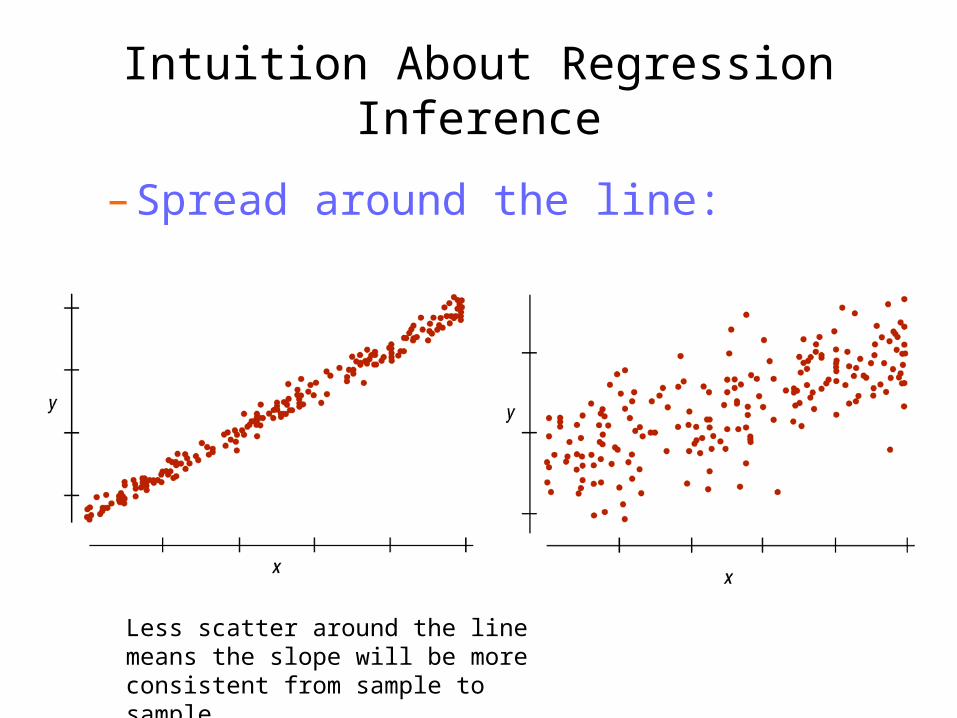
– Spread around the line:

Less scatter around the line means the slope will be more consistent from sample to sample.


– Spread of the x’s: A large standard deviation of x provides a more stable regression.


– Sample size: Having a larger sample size, n, gives more consistent estimates.

Standard Error for the Slope

• Three aspects of the scatterplot affect the standard error of the regression slope: – spread around the line, se

– spread of x values, sx

– sample size, n.• The formula for the standard error (which you

will probably never have to calculate by hand) is: 1

1e

x

sSE b

n s

Sampling Distribution for Regression Slopes

• When the conditions are met, the standardized estimated regression slope

follows a Student’s t-model with n – 2 degrees of freedom.

1 1

1

bt

SE b

Sampling Distribution for Regression Slopes

• We estimate the standard error with

where:

–

– n is the number of data values– sx is the ordinary standard deviation of the x-values.

11

e

x

sSE b

n s

2ˆ

2e

y ys

n

What About the Intercept?

• The same reasoning applies for the intercept.

• We can writebut we rarely use this fact for anything.

• The intercept usually isn’t interesting. Most hypothesis tests and confidence intervals for regression are about the slope.

b0 0

SE(b0): tn 2

Regression Inference

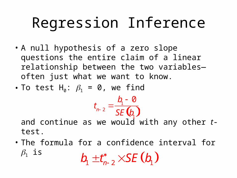
• A null hypothesis of a zero slope questions the entire claim of a linear relationship between the two variables—often just what we want to know.

• To test H0: 1 = 0, we find

and continue as we would with any other t-test.• The formula for a confidence interval for 1 is

tn 2

b

1 0

SE b1

1 2 1nb t SE b

*Standard Errors for Predicted Values

• Once we have a useful regression, how can we indulge our natural desire to predict, without being irresponsible?

• Now we have standard errors—we can use those to construct a confidence interval for the predictions, smudging the results in the right way to report our uncertainty honestly.

Documents

Inferences for Regression Chapter 27. An Example: Body Fat and Waist Size Our chapter example revolves around the relationship between % body fat and