Embed Size (px)
Citation preview
Inference for RegressionInference for RegressionSimple Linear Regression
IPS Chapter 10.1
© 2009 W.H. Freeman and Company

Objectives (IPS Chapter 10.1)
Simple linear regression
Statistical model for linear regression
Estimating the regression parameters
Confidence interval for regression parameters
Significance test for the slopeSignificance test for the slope
Confidence interval for µy
Prediction intervals
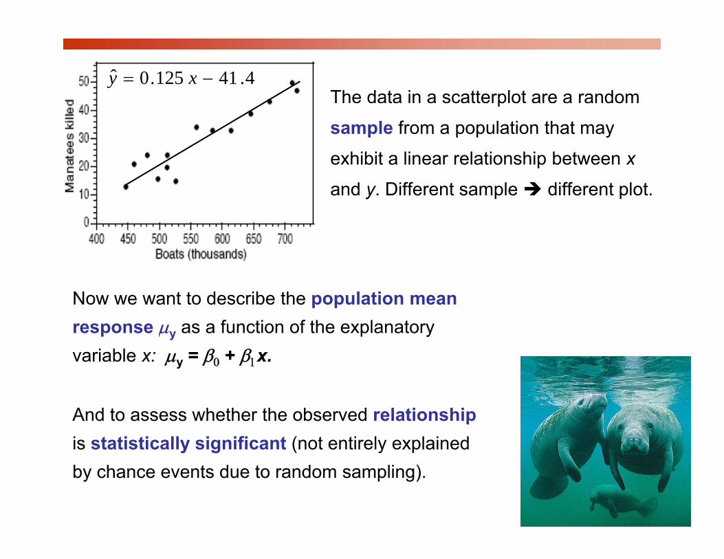
The data in a scatterplot are a random ˆ y = 0.125 x − 41 .4
p
sample from a population that may
exhibit a linear relationship between x
and y. Different sample different plot.
Now we want to describe the population mean response μy as a function of the explanatory variable x: μy = β0 + β1x.
And to assess whether the observed relationship is statistically significant (not entirely explained by chance events due to random sampling).

Statistical model for linear regressionIn the population, the linear regression equation is μy = β0 + β1x.
Sample data then fits the model:
Data = fit + residualyi = (β0 + β1xi) + (εi)
where the εi are independent and N ll di t ib t d N(0 )Normally distributed N(0,σ).
Linear regression assumes equal variance of y(σ is the same for all values of x).

μ = β + β x
Estimating the parameters
μy = β0 + β1x
The intercept β0, the slope β1, and the standard deviation σ of y are the
unknown parameters of the regression model We rely on the randomunknown parameters of the regression model. We rely on the random
sample data to provide unbiased estimates of these parameters.
The value of ŷ from the least-squares regression line is really a prediction
of the mean value of y (μy) for a given value of x.
The least-squares regression line (ŷ = b0 + b1x) obtained from sample data
is the best estimate of the true population regression line (μy = β0 + β1x).
ŷ unbiased estimate for mean response μy
b0 unbiased estimate for intercept β0
b1 unbiased estimate for slope β1
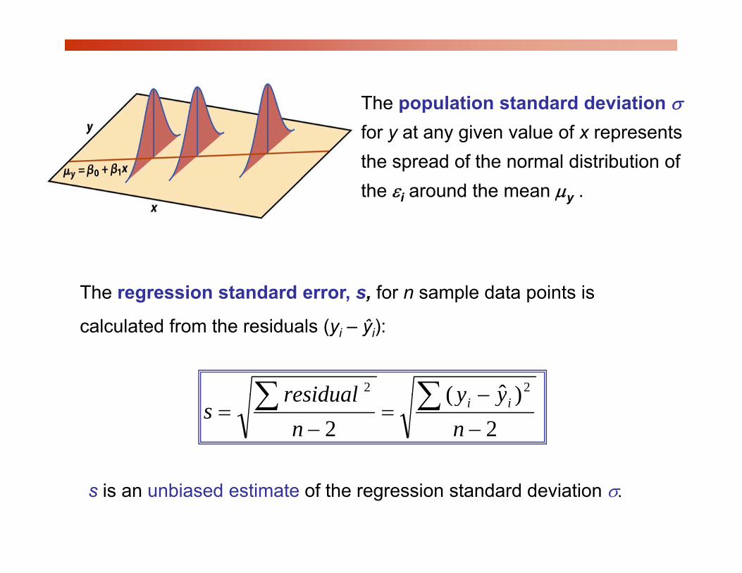
The population standard deviation σThe population standard deviation σfor y at any given value of x represents the spread of the normal distribution of the εi around the mean μy .
The regression standard error, s, for n sample data points is
calculated from the residuals (y ŷ ):calculated from the residuals (yi – ŷi):
)ˆ( 22 ∑∑ yyresidual2
)(
2 −−
=−
= ∑∑n
yyn
residuals ii
s is an unbiased estimate of the regression standard deviation σ.
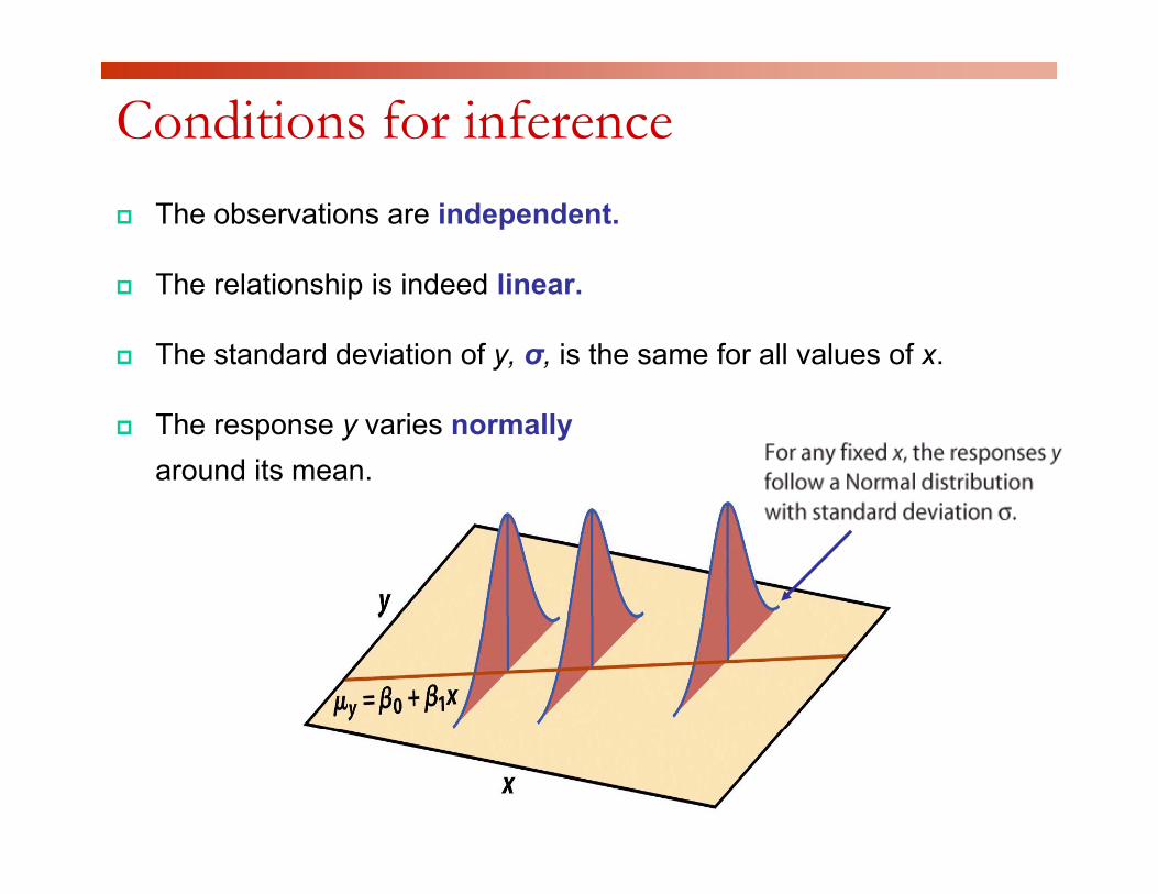
Conditions for inferenceThe observations are independent.
Th l ti hi i i d d liThe relationship is indeed linear.
The standard deviation of y, σ, is the same for all values of x.
The response y varies normallyaround its mean.
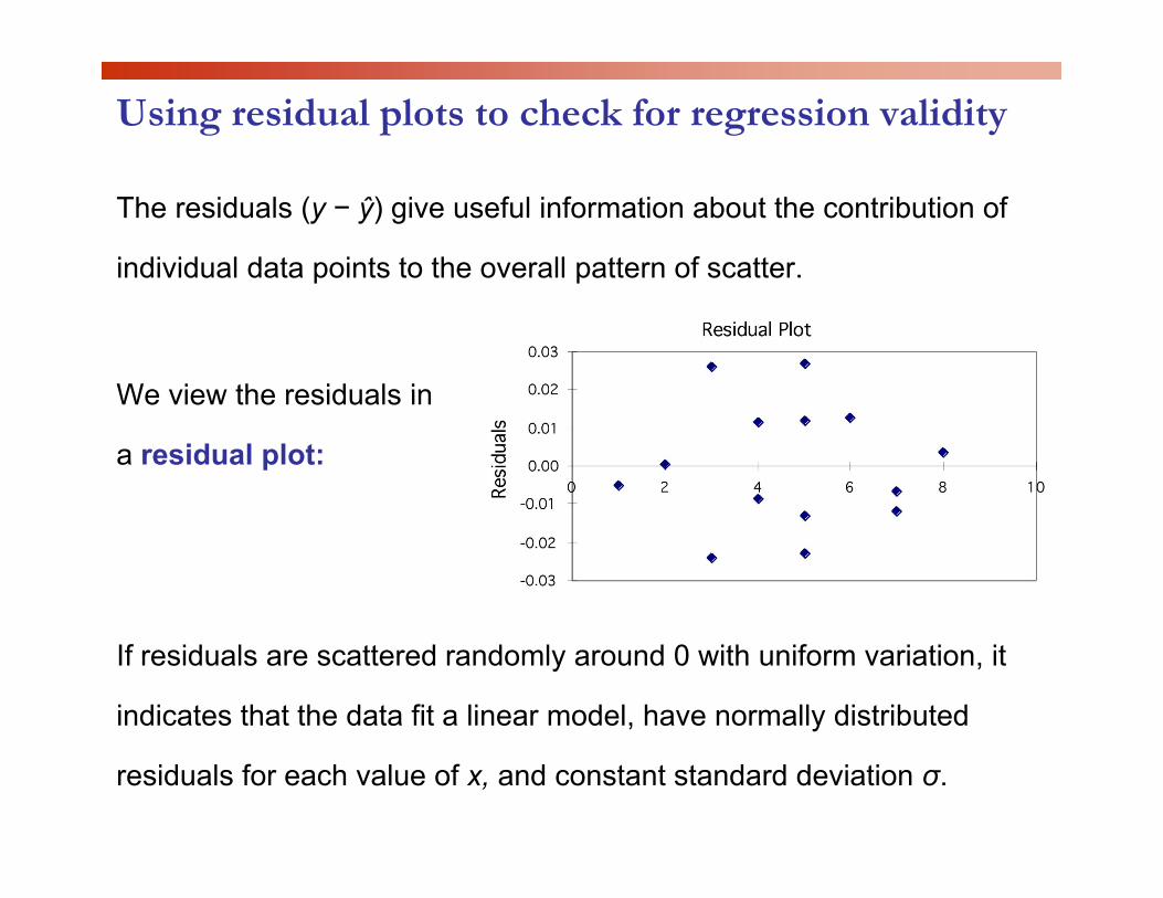
Using residual plots to check for regression validity
The residuals (y − ŷ) give useful information about the contribution of
individual data points to the overall pattern of scatter. p p
We view the residuals inWe view the residuals in
a residual plot:
If residuals are scattered randomly around 0 with uniform variation, it
indicates that the data fit a linear model, have normally distributed
residuals for each value of x, and constant standard deviation σ.
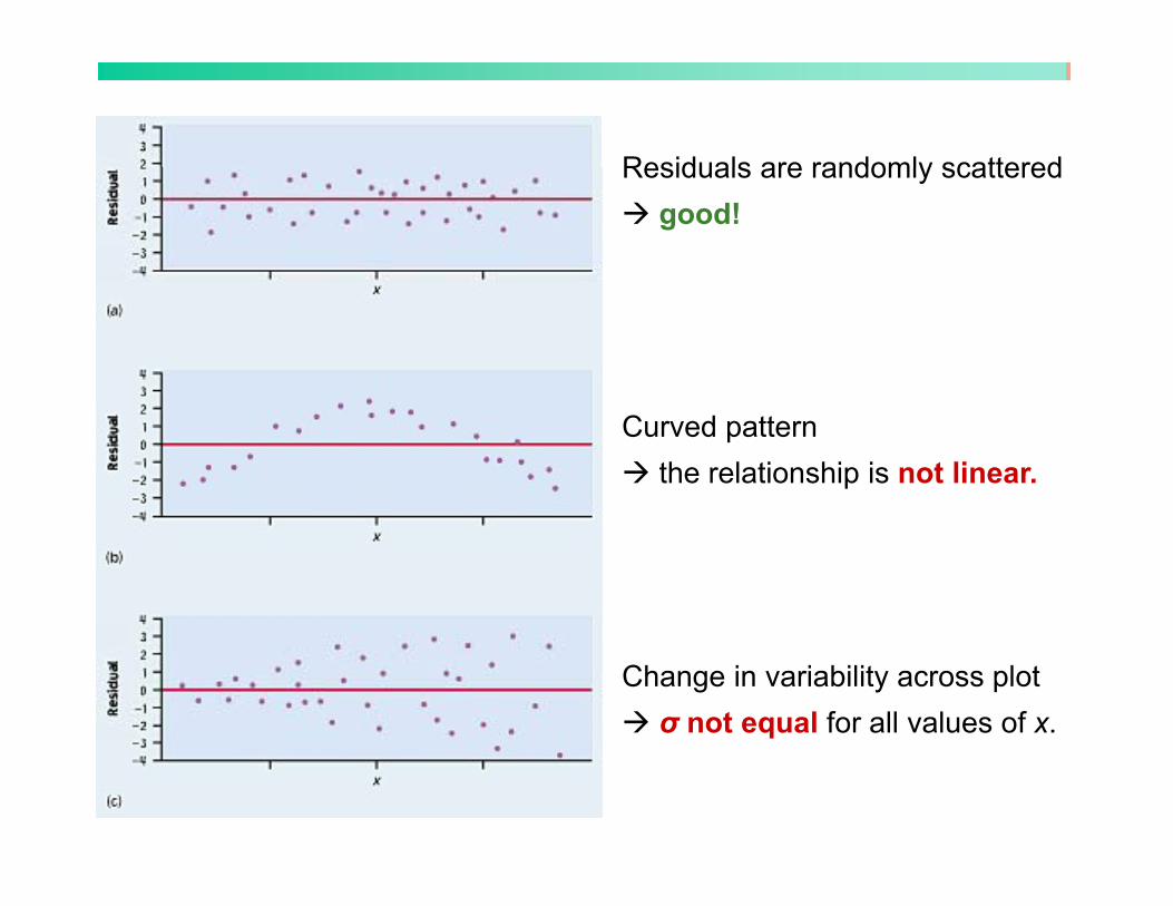
Residuals are randomly scatteredResiduals are randomly scattered good!
Curved pattern the relationship is not linear.
Change in variability across plotσ not equal for all values of x.
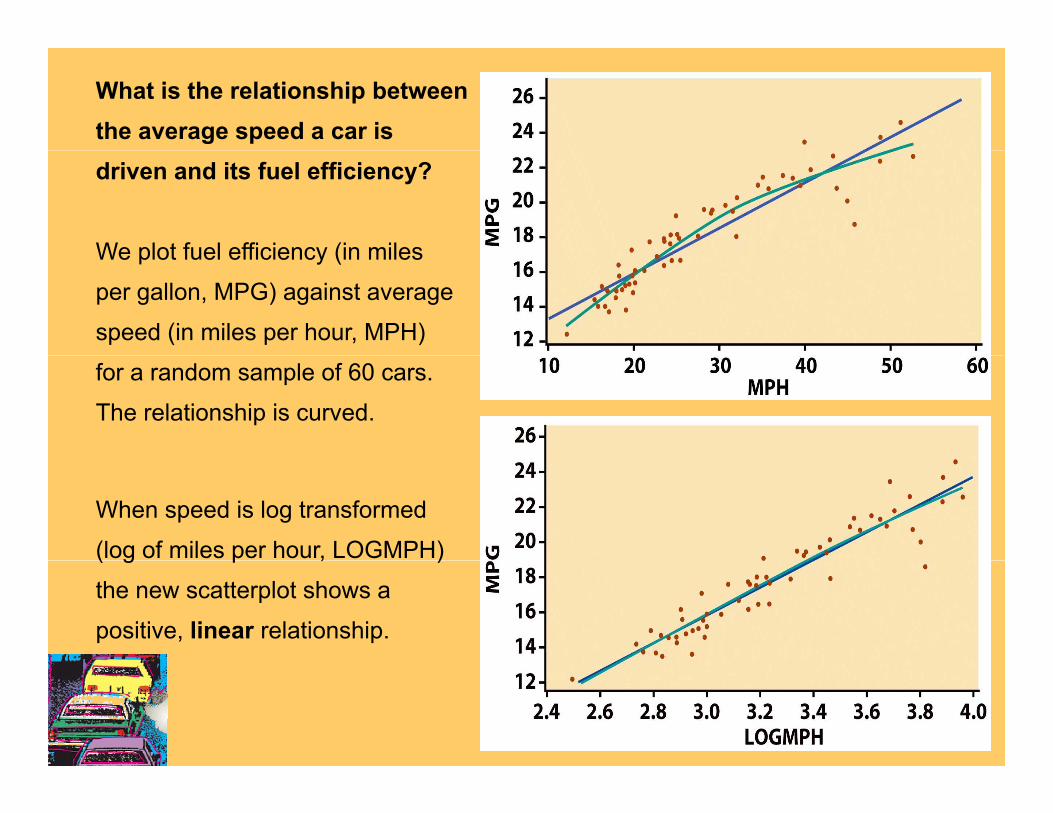
What is the relationship between the average speed a car is driven and its fuel efficiency?
We plot fuel efficiency (in milesWe plot fuel efficiency (in miles
per gallon, MPG) against average
speed (in miles per hour, MPH)
for a random sample of 60 cars.
The relationship is curved.
When speed is log transformed
(log of miles per hour, LOGMPH) ( g p , )
the new scatterplot shows a
positive, linear relationship.
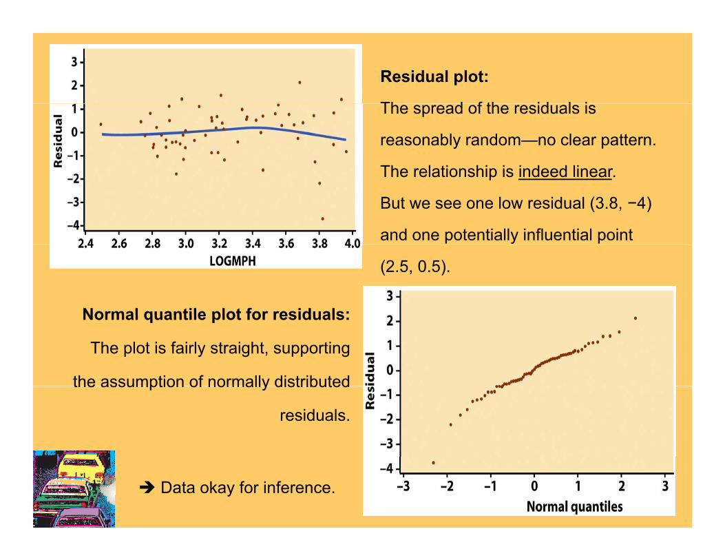
Residual plot:
Th d f th id l iThe spread of the residuals is
reasonably random—no clear pattern.
The relationship is indeed linearThe relationship is indeed linear.
But we see one low residual (3.8, −4)
and one potentially influential point
(2.5, 0.5).
Normal quantile plot for residuals:Normal quantile plot for residuals:
The plot is fairly straight, supporting
the assumption of normally distributedthe assumption of normally distributed
residuals.
Data okay for inference.
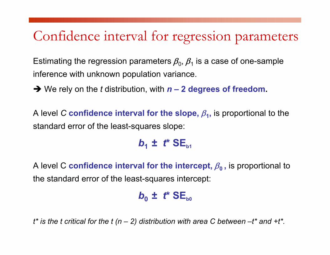
Confidence interval for regression parametersEstimating the regression parameters β0, β1 is a case of one-sample inference with unknown population variance.
We rely on the t distribution, with n – 2 degrees of freedom.
A le el C confidence inter al for the slope β is proportional to theA level C confidence interval for the slope, β1, is proportional to the standard error of the least-squares slope:
b ± t* SEb1 ± t SEb1
A level C confidence interval for the intercept, β0 , is proportional to th t d d f th l t i t tthe standard error of the least-squares intercept:
b0 ± t* SEb0
t* is the t critical for the t (n – 2) distribution with area C between –t* and +t*.
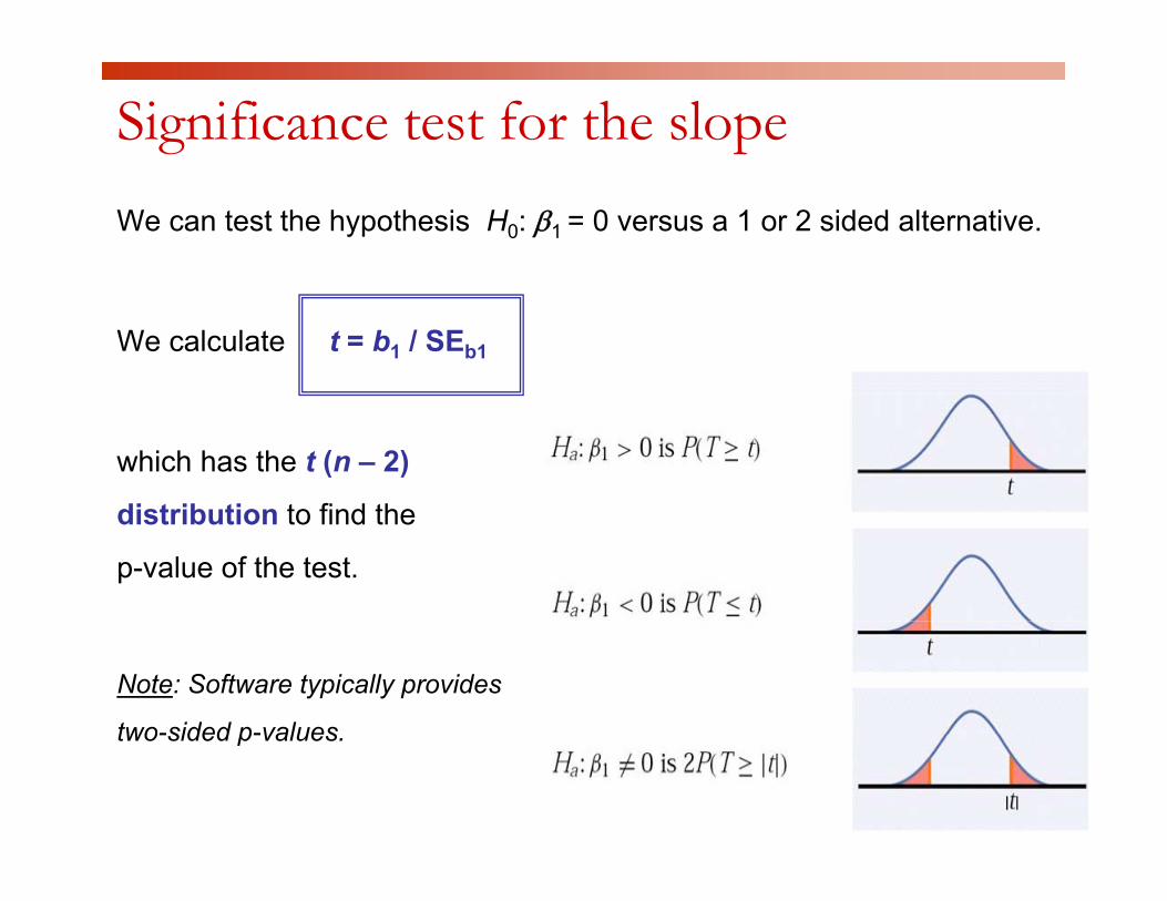
Significance test for the slopeWe can test the hypothesis H0: β1 = 0 versus a 1 or 2 sided alternative.
We calculate t = b1 / SEb1
which has the t (n – 2)
di t ib ti t fi d thdistribution to find the
p-value of the test.
Note: Software typically provides
two-sided p-valuestwo-sided p-values.

Testing the hypothesis of no relationship
We may look for evidence of a significant relationship between
variables x and y in the population from which our data were drawn.
For that, we can test the hypothesis that the regression slope
parameter β is equal to zeroparameter β is equal to zero.
H0: β1 = 0 vs. H0: β1 ≠ 0
Testing H0: β1 = 0 also allows to test the hypothesis of no 1slope ys
b r=correlation between x and y in the population. 1slope
x
b rs
Note: A test of hypothesis for β0 is irrelevant (β0 is often not even achievable).
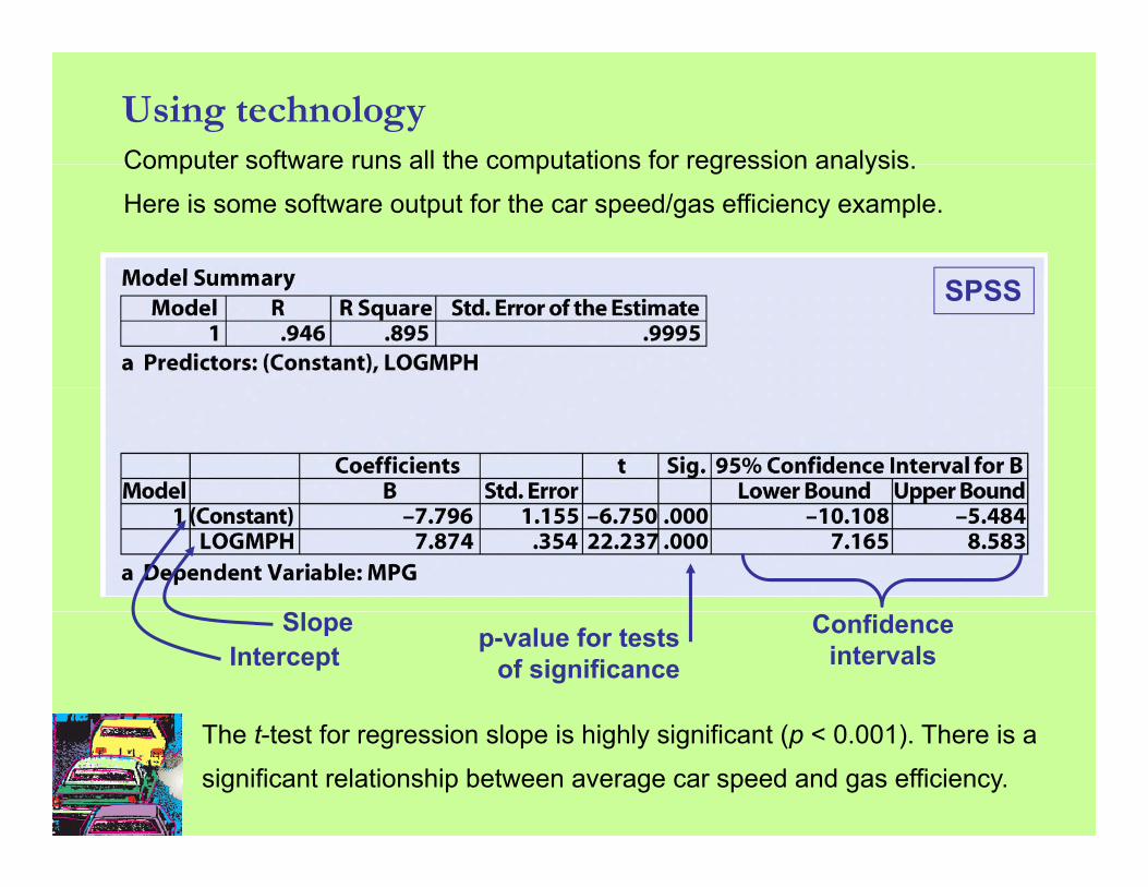
Using technologyComputer software runs all the computations for regression analysisComputer software runs all the computations for regression analysis.
Here is some software output for the car speed/gas efficiency example.
SPSS
SlopeIntercept
p-value for tests of significance
Confidence intervals
The t-test for regression slope is highly significant (p < 0.001). There is a
significant relationship between average car speed and gas efficiency.
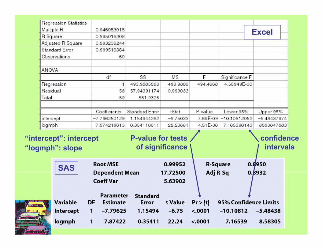
Excel
“intercept”: intercept P-value for tests confidence
SAS
intercept : intercept“logmph”: slope
P value for tests of significance
confidence intervals
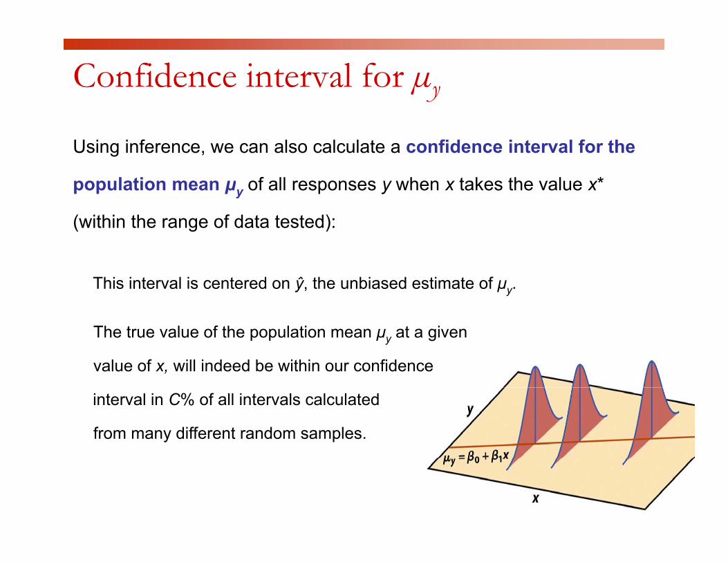
Confidence interval for µyUsing inference, we can also calculate a confidence interval for the
population mean μy of all responses y when x takes the value x*
(within the range of data tested):
This interval is centered on ŷ, the unbiased estimate of μy.
The true value of the population mean μy at a given
value of x, will indeed be within our confidence
interval in C% of all intervals calculated
from many different random samples.
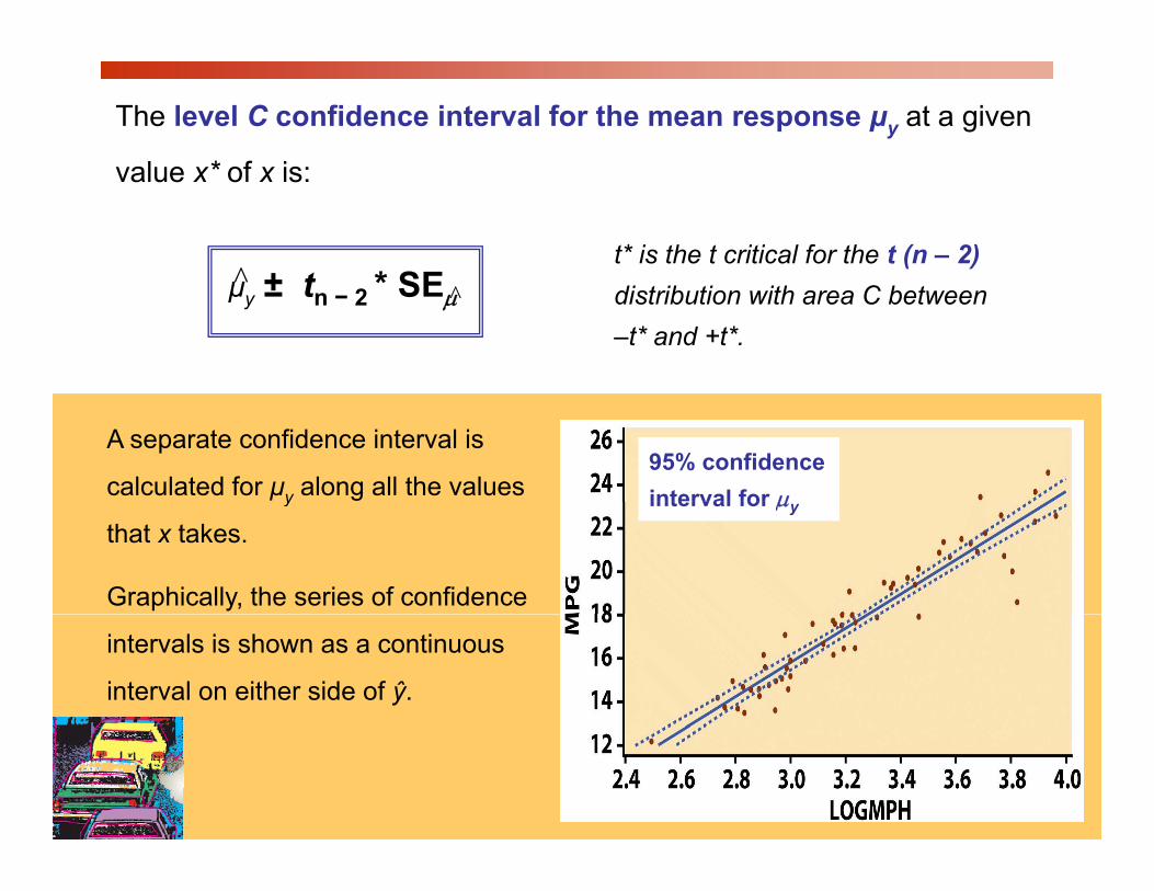
The level C confidence interval for the mean response μy at a given
l * f ivalue x* of x is:
± t * SEt* is the t critical for the t (n – 2)
μ̂y ± tn − 2 * SEμ distribution with area C between –t* and +t*.
^^
A separate confidence interval is
calculated for μy along all the values 95% confidence interval for μy
that x takes.
Graphically, the series of confidence
interval for μy
intervals is shown as a continuous
interval on either side of ŷ.

Inference for predictionOne use of regression is for predicting the value of y, ŷ, for any value
of x within the range of data tested: ŷ = b0 + b1x.of x within the range of data tested: ŷ b0 b1x.
But the regression equation depends on the particular sample drawn.
More reliable predictions require statistical inference:More reliable predictions require statistical inference:
To estimate an individual response y for a given value of x, we use a o est ate a d dua espo se y o a g e a ue o , e use a
prediction interval.
If we randomly sampled many times, there y p y
would be many different values of y
obtained for a particular x following
N(0, σ) around the mean response µy.

The level C prediction interval for a single observation on y when x
takes the value x* is:
ŷ t* SEt* is the t critical for the t (n – 2)di t ib ti ith C b tŷ ± t*n − 2 SEŷ distribution with area C between –t* and +t*.
The prediction interval represents
mainly the error from the normal 95% prediction i t l f ŷdistribution of the residuals εi.
Graphically, the series confidence
interval for ŷ
Graphically, the series confidence
intervals are shown as a continuous
interval on either side of ŷ.
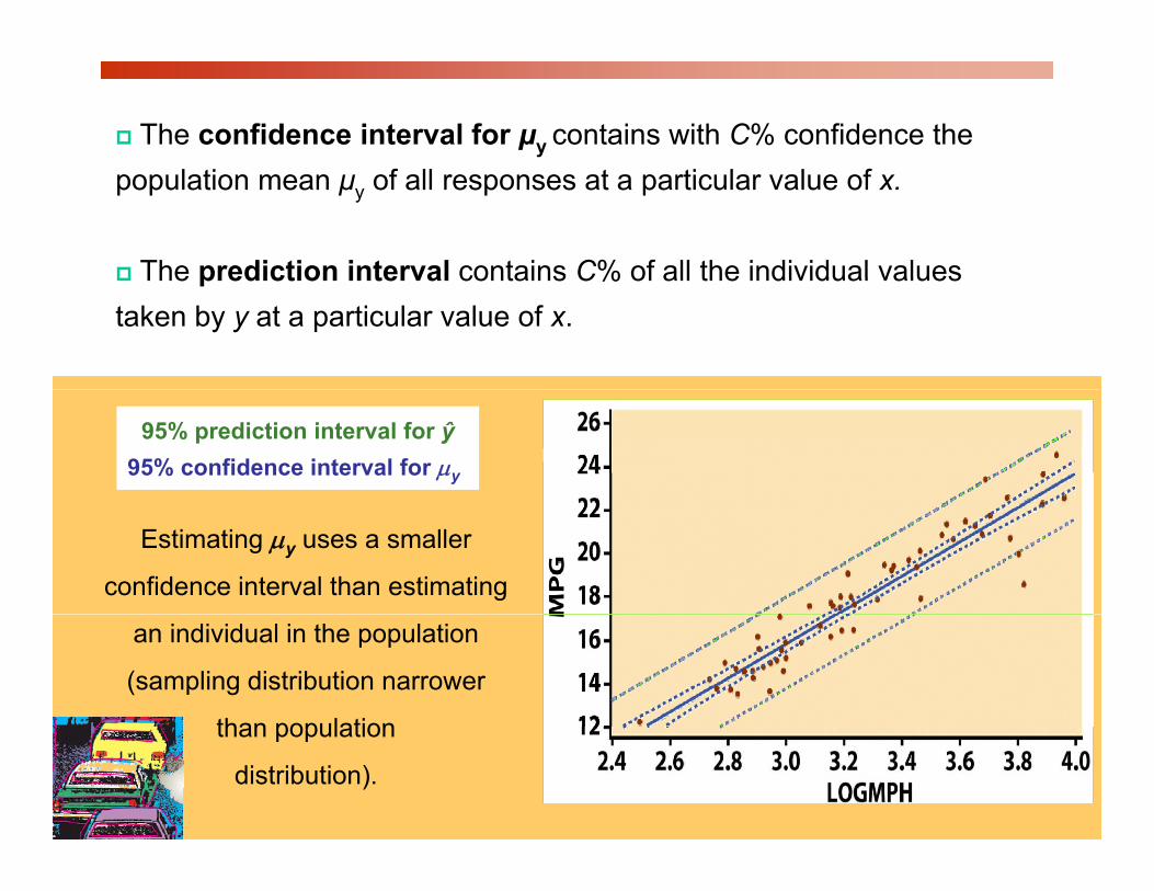
The confidence interval for μy contains with C% confidence the population mean μy of all responses at a particular value of x.
The prediction interval contains C% of all the individual valuesThe prediction interval contains C% of all the individual values taken by y at a particular value of x.
95% prediction interval for ŷ95% confidence interval for μy
Estimating μy uses a smaller
confidence interval than estimating
an individual in the population
(sampling distribution narrower
than populationthan population
distribution).

1918 influenza epidemic
10000 800
1918 flu epidemics
6000700080009000
10000
agno
sed
500600700800
repo
rted
1918 influenza epidemic 10002000300040005000
# ca
ses
dia
100200300400
# de
aths
r
1918 influenza epidemicDate # Cases # Deathsweek 1 36 0week 2 531 0week 3 4233 130
eek 4 8682 552
01000
week 1
week 3
week 5
week 7
week 9
week 1
1wee
k 13
week 1
5wee
k 17
0
week 4 8682 552week 5 7164 738week 6 2229 414week 7 600 198week 8 164 90
# Cases # Deaths
The line graph suggests that 7 to 9% of those week 9 57 56week 10 722 50week 11 1517 71week 12 1828 137week 13 1539 178
diagnosed with the flu died within about a week of diagnosis.
We look at the relationship between the number ofweek 13 1539 178week 14 2416 194week 15 3148 290week 16 3465 310week 17 1440 149
We look at the relationship between the number of deaths in a given week and the number of new
diagnosed cases one week earlier.
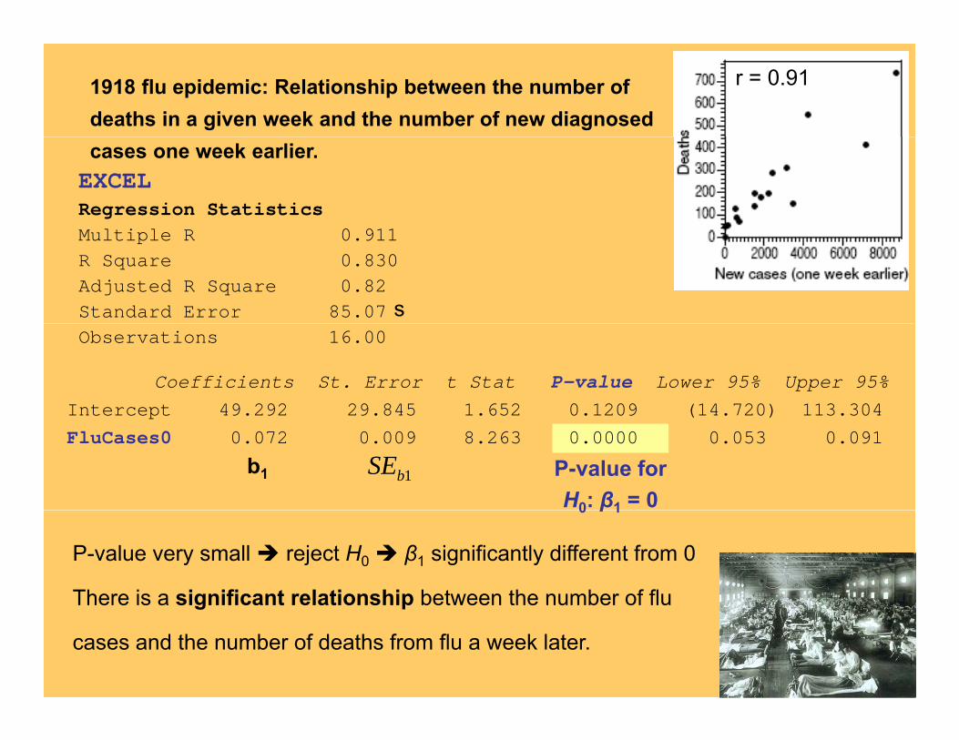
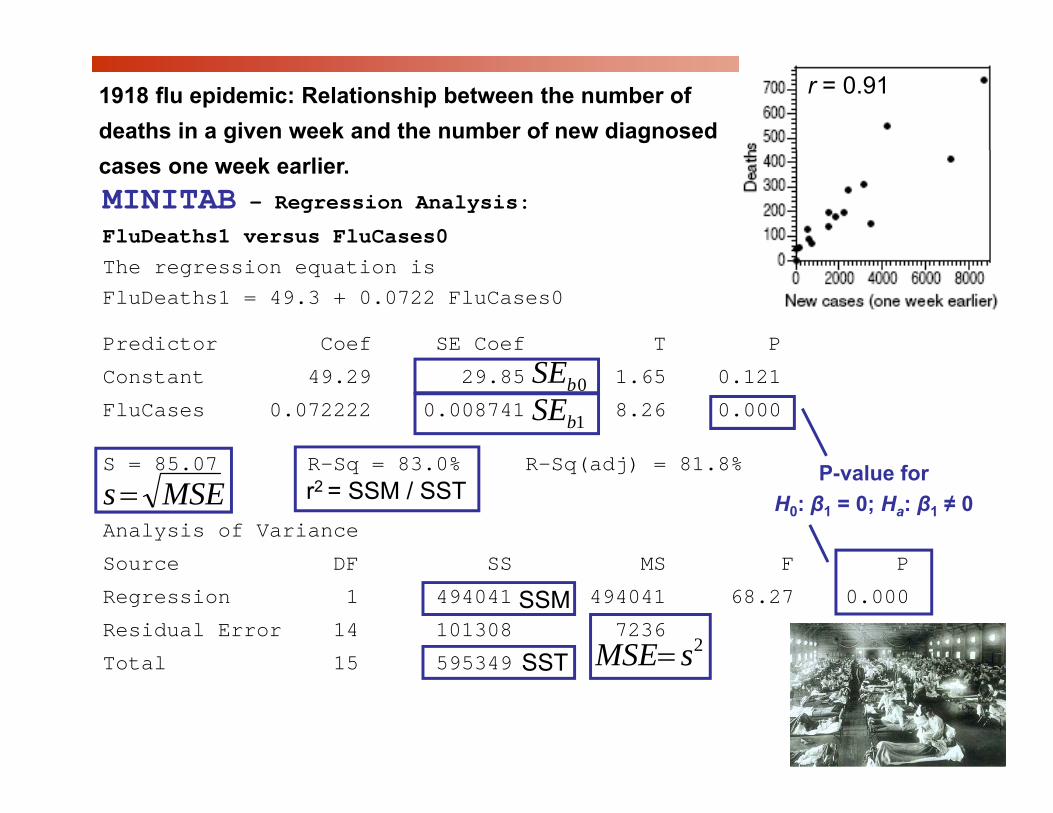
1918 flu epidemic: Relationship between the number of deaths in a given week and the number of new diagnosed
r = 0.91
EXCELRegression StatisticsM lti l R 0 911
cases one week earlier.
Multiple R 0.911 R Square 0.830 Adjusted R Square 0.82 Standard Error 85.07 sObservations 16.00
Coefficients St. Error t Stat P-value Lower 95% Upper 95% Intercept 49.292 29.845 1.652 0.1209 (14.720) 113.304 p ( )FluCases0 0.072 0.009 8.263 0.0000 0.053 0.091
1bSE P-value for H0: β1 = 0
b1
0 β1
P-value very small reject H0 β1 significantly different from 0
There is a significant relationship between the number of fluThere is a significant relationship between the number of flu
cases and the number of deaths from flu a week later.
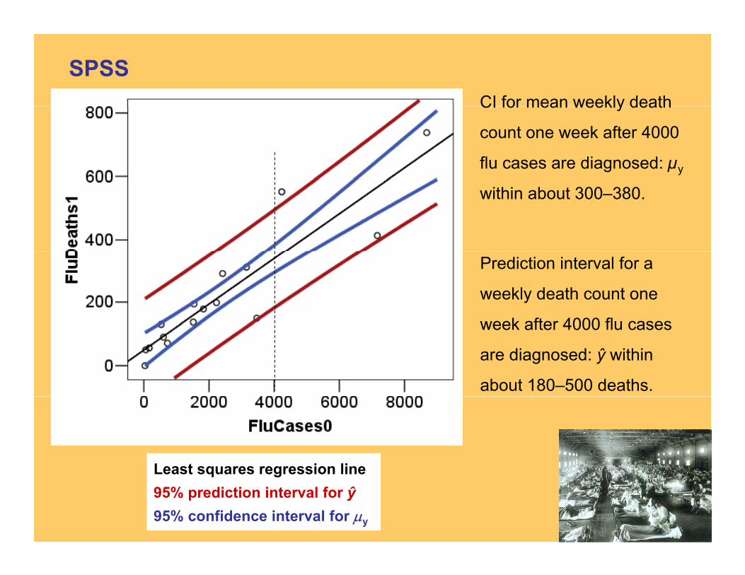
SPSSCI for mean weekly deathCI for mean weekly death
count one week after 4000
flu cases are diagnosed: µy
within about 300–380.
Prediction interval for a
weekly death count one
week after 4000 flu casesweek after 4000 flu cases
are diagnosed: ŷ within
about 180–500 deaths.
Least squares regression lineLeast squares regression line95% prediction interval for ŷ95% confidence interval for μy
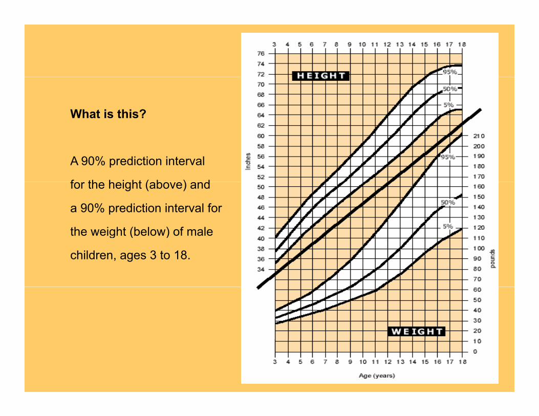
What is this?
A 90% prediction interval
f th h i ht ( b ) dfor the height (above) and
a 90% prediction interval for
the weight (below) of malethe weight (below) of male
children, ages 3 to 18.

Inference for RegressionInference for RegressionMore Detail about Simple Linear Regression
IPS Chapter 10.2
© 2009 W.H. Freeman and Company
Objectives (IPS Chapter 10.2)
Inference for regression—more details
Analysis of variance for regression
The ANOVA F test
Calculations for regression inferenceg
Inference for correlation
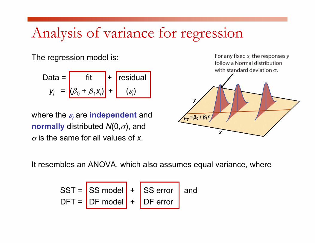
Analysis of variance for regressionThe regression model is:
D t fit + id lData = fit + residual
yi = (β0 + β1xi) + (εi)
where the εi are independent and normally distributed N(0,σ), and σ is the same for all values of xσ is the same for all values of x.
It resembles an ANOVA, which also assumes equal variance, where, q ,
SST = SS model + SS error and DFT = DF model + DF error
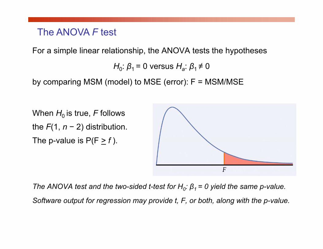
The ANOVA F test
For a simple linear relationship, the ANOVA tests the hypotheses
H0: β1 = 0 versus Ha: β1 ≠ 0
by comparing MSM (model) to MSE (error): F = MSM/MSE
When H0 is true, F follows
the F(1, n − 2) distribution.
The p value is P(F > f )The p-value is P(F > f ).
The ANOVA test and the two-sided t-test for H0: β1 = 0 yield the same p-value.
Software output for regression may provide t, F, or both, along with the p-value.p g y p , , , g p
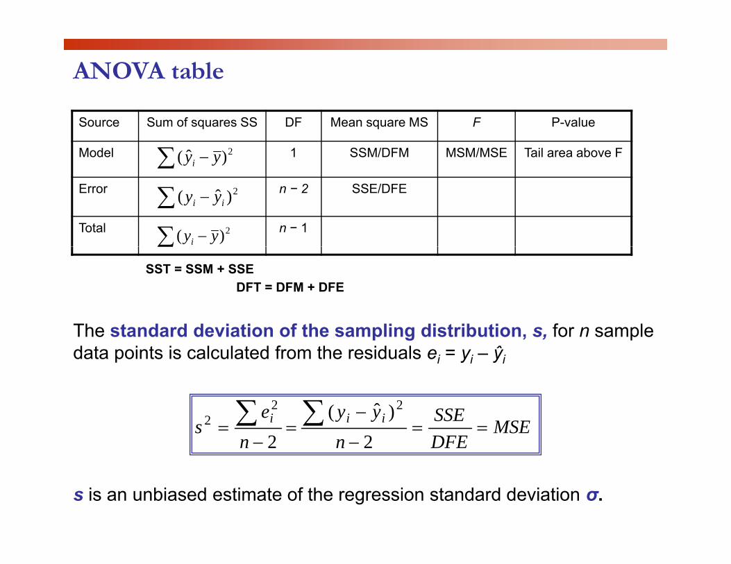
ANOVA table
Source Sum of squares SS DF Mean square MS F P-value
Model 1 SSM/DFM MSM/MSE Tail area above F∑ − 2)ˆ( yyi
Error n − 2 SSE/DFE
Total n − 1∑ − 2)( yyi
∑ − 2)ˆ( ii yy
∑SST = SSM + SSE
DFT = DFM + DFE
The standard deviation of the sampling distribution, s, for n sample data points is calculated from the residuals ei = yi – ŷi
MSEDFESSE
nyy
ne
s iii ==−
−=
−= ∑∑
2)ˆ(
2
222
s is an unbiased estimate of the regression standard deviation σ.
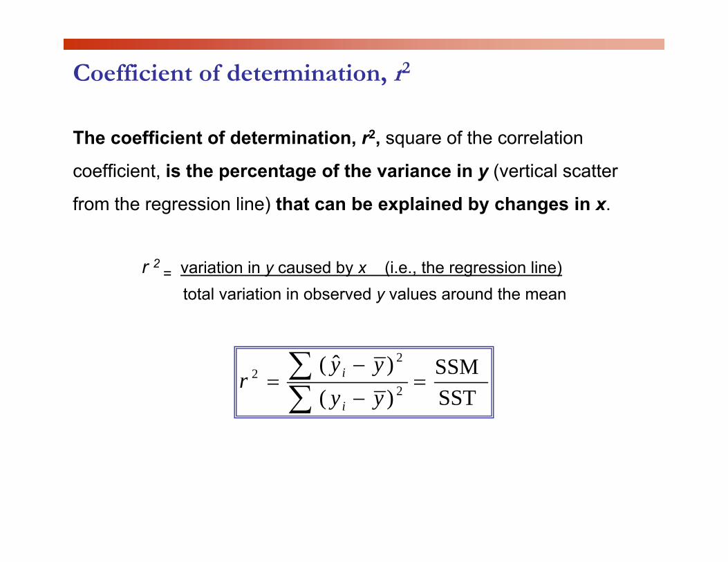
Coefficient of determination, r2
The coefficient of determination, r2, square of the correlation
coefficient is the percentage of the variance in y (vertical scattercoefficient, is the percentage of the variance in y (vertical scatter
from the regression line) that can be explained by changes in x.
r 2 = variation in y caused by x (i.e., the regression line)
total variation in observed y values around the mean
SSM)ˆ(2
22 =
−=∑∑ yy
r i
SST)( 2−∑ yyr
i
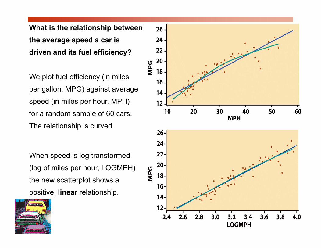
What is the relationship between the average speed a car is driven and its fuel efficiency?
We plot fuel efficiency (in milesWe plot fuel efficiency (in miles
per gallon, MPG) against average
speed (in miles per hour, MPH)
for a random sample of 60 cars.
The relationship is curved.
When speed is log transformed
(log of miles per hour, LOGMPH) ( g p , )
the new scatterplot shows a
positive, linear relationship.
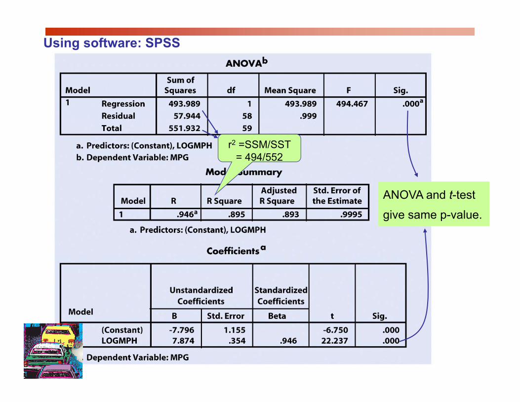
Using software: SPSS
r2 =SSM/SST = 494/552
ANOVA and t-test
give same p-value.
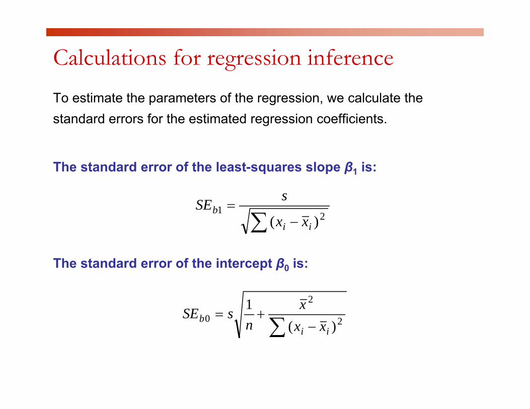
Calculations for regression inferenceTo estimate the parameters of the regression, we calculate the standard errors for the estimated regression coefficients.
The standard error of the least-squares slope β1 is:
)( 21
∑ −=
iib
xx
sSE
The standard error of the intercept β0 is:
∑
∑ −+= 2
2
0 )(1
iib xx
xn
sSE∑ )( ii

To estimate or predict future responses, we calculate the following standard errors
The standard error of the mean response µy is:
The standard error for predicting an individual response ŷ is:

1918 influenza epidemic
10000 800
1918 flu epidemics
6000700080009000
10000
agno
sed
500600700800
repo
rted
1918 influenza epidemic 10002000300040005000
# ca
ses
dia
100200300400
# de
aths
r
1918 influenza epidemicDate # Cases # Deathsweek 1 36 0week 2 531 0week 3 4233 130
eek 4 8682 552
01000
week 1
week 3
week 5
week 7
week 9
week 1
1wee
k 13
week 1
5wee
k 17
0
week 4 8682 552week 5 7164 738week 6 2229 414week 7 600 198week 8 164 90
# Cases # Deaths
The line graph suggests that about 7 to 8% of thoseweek 9 57 56week 10 722 50week 11 1517 71week 12 1828 137week 13 1539 178
The line graph suggests that about 7 to 8% of those diagnosed with the flu died within about a week of diagnosis. We look at the relationship between the
f fweek 13 1539 178week 14 2416 194week 15 3148 290week 16 3465 310week 17 1440 149
number of deaths in a given week and the number of new diagnosed cases one week earlier.
r = 0.911918 flu epidemic: Relationship between the number of deaths in a given week and the number of new diagnosed
MINITAB - Regression Analysis:
FluDeaths1 versus FluCases0
cases one week earlier.
The regression equation isFluDeaths1 = 49.3 + 0.0722 FluCases0
Predictor Coef SE Coef T P
Constant 49.29 29.85 1.65 0.121
FluCases 0.072222 0.008741 8.26 0.000
S 85 07 R S 83 0% R S ( dj) 81 8%
1bSE0bSE
S = 85.07 R-Sq = 83.0% R-Sq(adj) = 81.8%
Analysis of Variance
So rce DF SS MS F P
MSEs= P-value for
H0: β1 = 0; Ha: β1 ≠ 0r2 = SSM / SST
Source DF SS MS F P
Regression 1 494041 494041 68.27 0.000
Residual Error 14 101308 7236
Total 15 5953492sMSE=
SSM
SSTTotal 15 595349 sMSESST
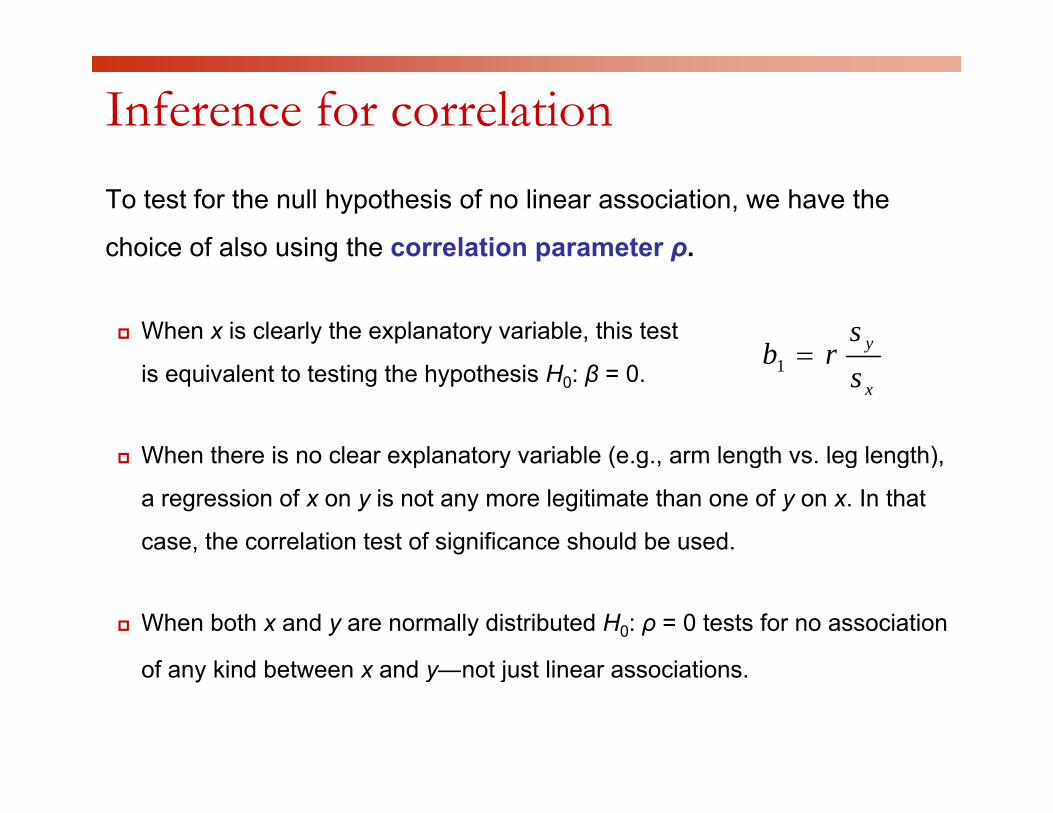
Inference for correlationTo test for the null hypothesis of no linear association, we have the
choice of also using the correlation parameter ρ.choice of also using the correlation parameter ρ.
When x is clearly the explanatory variable, this test ysb r=
is equivalent to testing the hypothesis H0: β = 0.
When there is no clear explanatory variable (e g arm length vs leg length)
1x
b rs
=
When there is no clear explanatory variable (e.g., arm length vs. leg length),
a regression of x on y is not any more legitimate than one of y on x. In that
case, the correlation test of significance should be used.
When both x and y are normally distributed H0: ρ = 0 tests for no association
f ki d b t d t j t li i tiof any kind between x and y—not just linear associations.

The test of significance for ρ uses the one-sample t-test for: H0: ρ = 0.g ρ p 0 ρ
We compute the t statisticsfor sample size n and
2r nt −=for sample size n and
correlation coefficient r.21
tr−
The p-value is the area
under t (n – 2) for values of
T as extreme as t or more
in the direction of Ha:
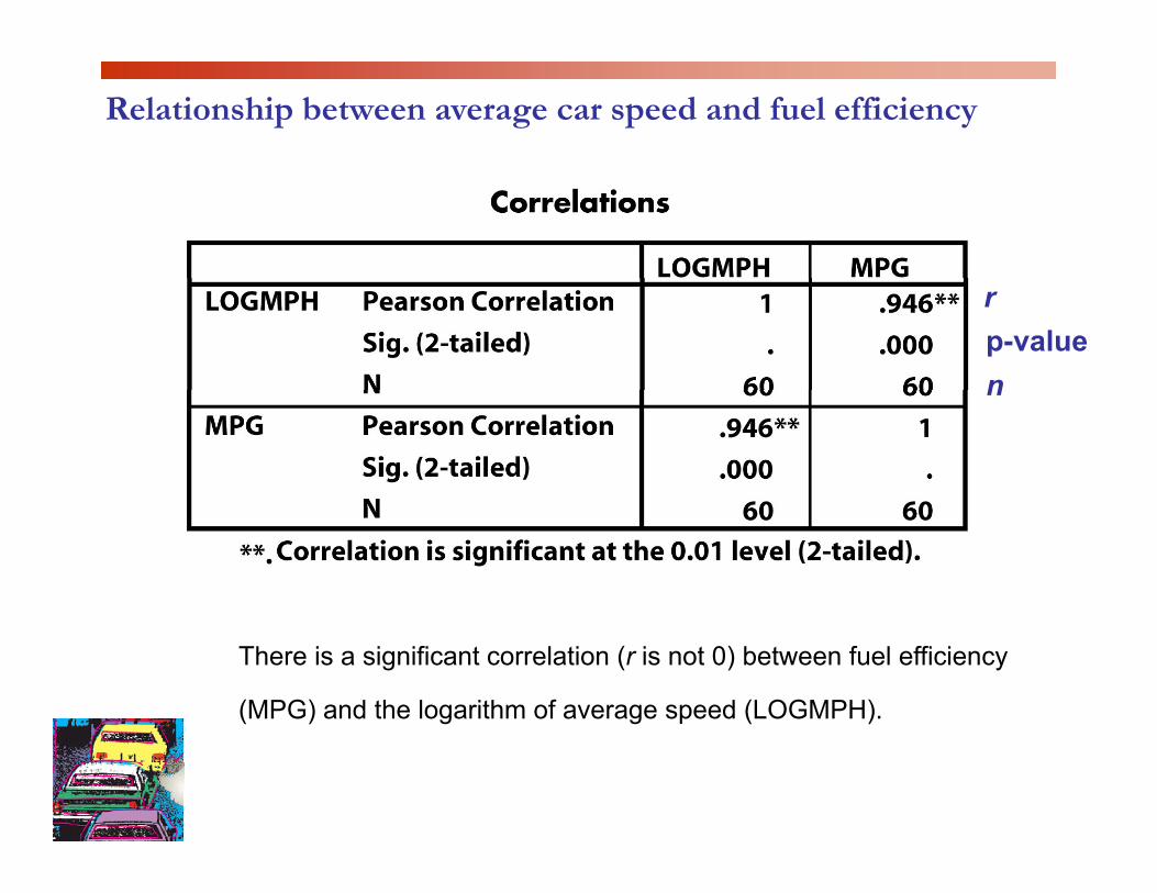
Relationship between average car speed and fuel efficiency
rp-valuenn
There is a significant correlation (r is not 0) between fuel efficiency
(MPG) and the logarithm of average speed (LOGMPH).