Embed Size (px)
Citation preview
Inference and Representation
David Sontag
New York University
Lecture 8, Nov. 3, 2015
David Sontag (NYU) Inference and Representation Lecture 8, Nov. 3, 2015 1 / 19
Latent Dirichlet allocation (LDA)
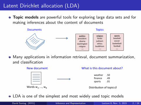
Topic models are powerful tools for exploring large data sets and formaking inferences about the content of documents
!"#$%&'() *"+,#)
+"/,9#)1+.&),3&'(1"65%51
:5)2,'0("'1.&/,0,"'1-
.&/,0,"'12,'3$14$3,5)%1&(2,#)1
6$332,)%1
)+".()165)&65//1)"##&.1
65)7&(65//18""(65//1
- -
Many applications in information retrieval, document summarization,and classification
Complexity+of+Inference+in+Latent+Dirichlet+Alloca6on+David+Sontag,+Daniel+Roy+(NYU,+Cambridge)+
W66+Topic+models+are+powerful+tools+for+exploring+large+data+sets+and+for+making+inferences+about+the+content+of+documents+
Documents+ Topics+poli6cs+.0100+
president+.0095+obama+.0090+
washington+.0085+religion+.0060+
Almost+all+uses+of+topic+models+(e.g.,+for+unsupervised+learning,+informa6on+retrieval,+classifica6on)+require+probabilis)c+inference:+
New+document+ What+is+this+document+about?+
Words+w1,+…,+wN+ ✓Distribu6on+of+topics+
�t =�
p(w | z = t)
…+
religion+.0500+hindu+.0092+
judiasm+.0080+ethics+.0075+
buddhism+.0016+
sports+.0105+baseball+.0100+soccer+.0055+
basketball+.0050+football+.0045+
…+ …+
weather+ .50+finance+ .49+sports+ .01+
LDA is one of the simplest and most widely used topic models
David Sontag (NYU) Inference and Representation Lecture 8, Nov. 3, 2015 2 / 19
Generative model for a document in LDA
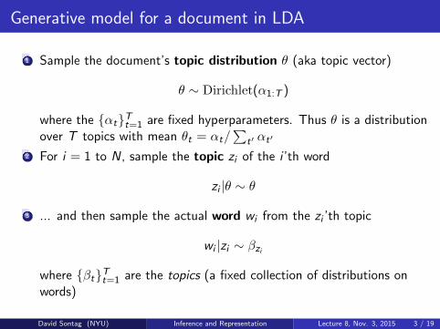
1 Sample the document’s topic distribution θ (aka topic vector)
θ ∼ Dirichlet(α1:T )
where the {αt}Tt=1 are fixed hyperparameters. Thus θ is a distributionover T topics with mean θt = αt/
∑t′ αt′
2 For i = 1 to N, sample the topic zi of the i ’th word
zi |θ ∼ θ
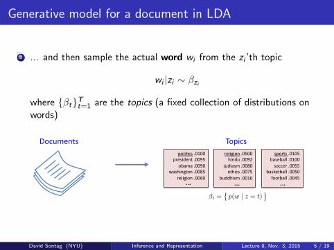
3 ... and then sample the actual word wi from the zi ’th topic
wi |zi ∼ βzi
where {βt}Tt=1 are the topics (a fixed collection of distributions onwords)
David Sontag (NYU) Inference and Representation Lecture 8, Nov. 3, 2015 3 / 19
Generative model for a document in LDA
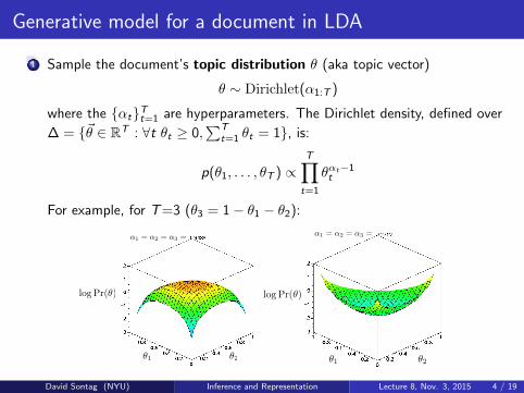
1 Sample the document’s topic distribution θ (aka topic vector)
θ ∼ Dirichlet(α1:T )
where the {αt}Tt=1 are hyperparameters. The Dirichlet density, defined over
∆ = {~θ ∈ RT : ∀t θt ≥ 0,∑T
t=1 θt = 1}, is:
p(θ1, . . . , θT ) ∝T∏
t=1
θαt−1t
For example, for T=3 (θ3 = 1− θ1 − θ2):
α1 = α2 = α3 =
θ1 θ2
log Pr(θ)
θ1 θ2
log Pr(θ)
α1 = α2 = α3 =
David Sontag (NYU) Inference and Representation Lecture 8, Nov. 3, 2015 4 / 19
Generative model for a document in LDA
3 ... and then sample the actual word wi from the zi ’th topic
wi |zi ∼ βzi
where {βt}Tt=1 are the topics (a fixed collection of distributions onwords)
Complexity+of+Inference+in+Latent+Dirichlet+Alloca6on+David+Sontag,+Daniel+Roy+(NYU,+Cambridge)+
W66+Topic+models+are+powerful+tools+for+exploring+large+data+sets+and+for+making+inferences+about+the+content+of+documents+
Documents+ Topics+poli6cs+.0100+
president+.0095+obama+.0090+
washington+.0085+religion+.0060+
Almost+all+uses+of+topic+models+(e.g.,+for+unsupervised+learning,+informa6on+retrieval,+classifica6on)+require+probabilis)c+inference:+
New+document+ What+is+this+document+about?+
Words+w1,+…,+wN+ ✓Distribu6on+of+topics+
�t =�
p(w | z = t)
…+
religion+.0500+hindu+.0092+
judiasm+.0080+ethics+.0075+
buddhism+.0016+
sports+.0105+baseball+.0100+soccer+.0055+
basketball+.0050+football+.0045+
…+ …+
weather+ .50+finance+ .49+sports+ .01+
David Sontag (NYU) Inference and Representation Lecture 8, Nov. 3, 2015 5 / 19
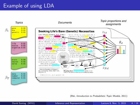
Example of using LDA
gene 0.04dna 0.02genetic 0.01.,,
life 0.02evolve 0.01organism 0.01.,,
brain 0.04neuron 0.02nerve 0.01...
data 0.02number 0.02computer 0.01.,,
Topics Documents Topic proportions andassignments
Figure 1: The intuitions behind latent Dirichlet allocation. We assume that somenumber of “topics,” which are distributions over words, exist for the whole collection (far left).Each document is assumed to be generated as follows. First choose a distribution over thetopics (the histogram at right); then, for each word, choose a topic assignment (the coloredcoins) and choose the word from the corresponding topic. The topics and topic assignmentsin this figure are illustrative—they are not fit from real data. See Figure 2 for topics fit fromdata.
model assumes the documents arose. (The interpretation of LDA as a probabilistic model isfleshed out below in Section 2.1.)
We formally define a topic to be a distribution over a fixed vocabulary. For example thegenetics topic has words about genetics with high probability and the evolutionary biologytopic has words about evolutionary biology with high probability. We assume that thesetopics are specified before any data has been generated.1 Now for each document in thecollection, we generate the words in a two-stage process.
1. Randomly choose a distribution over topics.
2. For each word in the document
(a) Randomly choose a topic from the distribution over topics in step #1.
(b) Randomly choose a word from the corresponding distribution over the vocabulary.
This statistical model reflects the intuition that documents exhibit multiple topics. Eachdocument exhibits the topics with different proportion (step #1); each word in each document
1Technically, the model assumes that the topics are generated first, before the documents.
3
θd
z1d
zNd
β1
βT
(Blei, Introduction to Probabilistic Topic Models, 2011)
David Sontag (NYU) Inference and Representation Lecture 8, Nov. 3, 2015 6 / 19
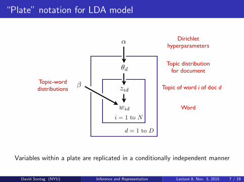
“Plate” notation for LDA model
α Dirichlet hyperparameters
i = 1 to N
d = 1 to D
θd
wid
zid
Topic distributionfor document
Topic of word i of doc d
Word
βTopic-worddistributions
Variables within a plate are replicated in a conditionally independent manner
David Sontag (NYU) Inference and Representation Lecture 8, Nov. 3, 2015 7 / 19
Outline of lecture
How to learn topic models?
Importance of hyperparametersChoosing number of topicsEvaluating topic models
Examples of extending LDA
Polylingual topic modelsAuthor-topic model
David Sontag (NYU) Inference and Representation Lecture 8, Nov. 3, 2015 8 / 19
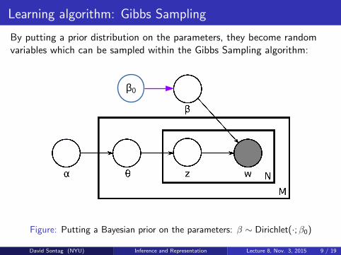
Learning algorithm: Gibbs Sampling
By putting a prior distribution on the parameters, they become randomvariables which can be sampled within the Gibbs Sampling algorithm:
α0
β0
Figure: Putting a Bayesian prior on the parameters: β ∼ Dirichlet(·;β0)
David Sontag (NYU) Inference and Representation Lecture 8, Nov. 3, 2015 9 / 19
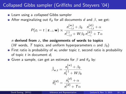
Collapsed Gibbs sampler (Griffiths and Steyvers ’04)
Learn using a collapsed Gibbs sampler
After marginalizing out θd for all documents d and β, we get:
P(zi = t | z−i ,w) ∝n(wi )−i ,t + β0
n(·)−i ,t + Wβ0
n(di )−i ,t + α
n(di )−i ,· + Tα
n derived from z, the assignments of words to topics(W words, T topics, and uniform hyperparameters α and β0)
First ratio is probability of wi under topic t, second ratio is probabilityof topic t in document diGiven a sample, can get an estimate for β and θd by:
β̂w ,t =n(w)t + β0
n(·)t + Wβ0
θ̂(d)t =
n(d)t + α
n(d)· + Tα
David Sontag (NYU) Inference and Representation Lecture 8, Nov. 3, 2015 10 / 19
Polylingual topic models (Mimno et al., EMNLP ’09)
Goal: topic models that are aligned across languages
Training data: corpora with multiple documents in each language
EuroParl corpus of parliamentary proceedings (11 western languages;exact translations)Wikipedia articles (12 languages; not exact translations)
How to do this?
David Sontag (NYU) Inference and Representation Lecture 8, Nov. 3, 2015 11 / 19
Polylingual topic models (Mimno et al., EMNLP ’09)
the contents of collections in unfamiliar languagesand identify trends in topic prevalence.
2 Related Work
Bilingual topic models for parallel texts withword-to-word alignments have been studied pre-viously using the HM-bitam model (Zhao andXing, 2007). Tam, Lane and Schultz (Tam etal., 2007) also show improvements in machinetranslation using bilingual topic models. Bothof these translation-focused topic models inferword-to-word alignments as part of their inferenceprocedures, which would become exponentiallymore complex if additional languages were added.We take a simpler approach that is more suit-able for topically similar document tuples (wheredocuments are not direct translations of one an-other) in more than two languages. A recent ex-tended abstract, developed concurrently by Ni etal. (Ni et al., 2009), discusses a multilingual topicmodel similar to the one presented here. How-ever, they evaluate their model on only two lan-guages (English and Chinese), and do not use themodel to detect differences between languages.They also provide little analysis of the differ-ences between polylingual and single-languagetopic models. Outside of the field of topic mod-eling, Kawaba et al. (Kawaba et al., 2008) usea Wikipedia-based model to perform sentimentanalysis of blog posts. They find, for example,that English blog posts about the Nintendo Wii of-ten relate to a hack, which cannot be mentioned inJapanese posts due to Japanese intellectual prop-erty law. Similarly, posts about whaling oftenuse (positive) nationalist language in Japanese and(negative) environmentalist language in English.
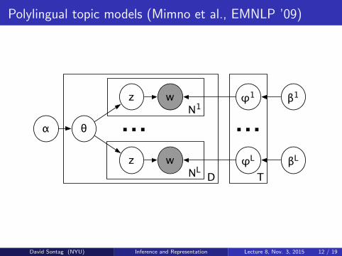
3 Polylingual Topic Model
The polylingual topic model (PLTM) is an exten-sion of latent Dirichlet allocation (LDA) (Blei etal., 2003) for modeling polylingual document tu-ples. Each tuple is a set of documents that areloosely equivalent to each other, but written in dif-ferent languages, e.g., corresponding Wikipediaarticles in French, English and German. PLTM as-sumes that the documents in a tuple share the sametuple-specific distribution over topics. This is un-like LDA, in which each document is assumed tohave its own document-specific distribution overtopics. Additionally, PLTM assumes that each“topic” consists of a set of discrete distributions
D
N1
TNL
...
w
α θ
wz
z
...
φ1
φL
β1
βL
Figure 1: Graphical model for PLTM.
over words—one for each language l = 1, . . . , L.In other words, rather than using a single set oftopics � = {�1, . . . ,�T }, as in LDA, there are Lsets of language-specific topics, �1, . . . ,�L, eachof which is drawn from a language-specific sym-metric Dirichlet with concentration parameter �l.
3.1 Generative ProcessA new document tuple w = (w1, . . . ,wL) is gen-erated by first drawing a tuple-specific topic dis-tribution from an asymmetric Dirichlet prior withconcentration parameter ↵ and base measure m:
✓ ⇠ Dir (✓,↵m). (1)
Then, for each language l, a latent topic assign-ment is drawn for each token in that language:
zl ⇠ P (zl |✓) =Q
n ✓zln. (2)
Finally, the observed tokens are themselves drawnusing the language-specific topic parameters:
wl ⇠ P (wl |zl,�l) =Q
n �lwl
n|zln. (3)
The graphical model is shown in figure 1.
3.2 InferenceGiven a corpus of training and test documenttuples—W and W 0, respectively—two possibleinference tasks of interest are: computing theprobability of the test tuples given the trainingtuples and inferring latent topic assignments fortest documents. These tasks can either be accom-plished by averaging over samples of �1, . . . ,�L
and ↵m from P (�1, . . . ,�L,↵m | W 0,�) or byevaluating a point estimate. We take the lat-ter approach, and use the MAP estimate for ↵mand the predictive distributions over words for�1, . . . ,�L. The probability of held-out docu-ment tuples W 0 given training tuples W is thenapproximated by P (W 0 |�1, . . . ,�L,↵m).
Topic assignments for a test document tuplew = (w1, . . . ,wL) can be inferred using Gibbs
881
David Sontag (NYU) Inference and Representation Lecture 8, Nov. 3, 2015 12 / 19
Learned topics
sampling. Gibbs sampling involves sequentiallyresampling each zl
n from its conditional posterior:
P (zln = t |w,z\l,n,�1, . . . ,�L,↵m)
/ �lwl
n|t(Nt)\l,n + ↵mtP
t Nt � 1 + ↵, (4)
where z\l,n is the current set of topic assignmentsfor all other tokens in the tuple, while (Nt)\l,n isthe number of occurrences of topic t in the tuple,excluding zl
n, the variable being resampled.
4 Results on Parallel Text
Our first set of experiments focuses on documenttuples that are known to consist of direct transla-tions. In this case, we can be confident that thetopic distribution is genuinely shared across alllanguages. Although direct translations in multi-ple languages are relatively rare (in contrast withcomparable documents), we use direct translationsto explore the characteristics of the model.
4.1 Data SetThe EuroParl corpus consists of parallel texts ineleven western European languages: Danish, Ger-man, Greek, English, Spanish, Finnish, French,Italian, Dutch, Portuguese and Swedish. Thesetexts consist of roughly a decade of proceedingsof the European parliament. For our purposes weuse alignments at the speech level rather than thesentence level, as in many translation tasks usingthis corpus. We also remove the twenty-five mostfrequent word types for efficiency reasons. Theremaining collection consists of over 121 millionwords. Details by language are shown in Table 1.
Table 1: Average document length, # documents, andunique word types per 10,000 tokens in the EuroParl corpus.
Lang. Avg. leng. # docs types/10kDA 160.153 65245 121.4DE 178.689 66497 124.5EL 171.289 46317 124.2EN 176.450 69522 43.1ES 170.536 65929 59.5FI 161.293 60822 336.2FR 186.742 67430 54.8IT 187.451 66035 69.5NL 176.114 66952 80.8PT 183.410 65718 68.2SV 154.605 58011 136.1
Models are trained using 1000 iterations ofGibbs sampling. Each language-specific topic–word concentration parameter �l is set to 0.01.
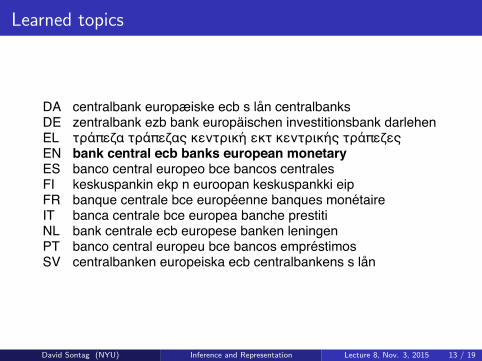
centralbank europæiske ecb s lån centralbanks zentralbank ezb bank europäischen investitionsbank darlehen τράπεζα τράπεζας κεντρική εκτ κεντρικής τράπεζες bank central ecb banks european monetary banco central europeo bce bancos centrales keskuspankin ekp n euroopan keskuspankki eip banque centrale bce européenne banques monétaire banca centrale bce europea banche prestiti bank centrale ecb europese banken leningen banco central europeu bce bancos empréstimos centralbanken europeiska ecb centralbankens s lån
børn familie udnyttelse børns børnene seksuel kinder kindern familie ausbeutung familien eltern παιδιά παιδιών οικογένεια οικογένειας γονείς παιδικής children family child sexual families exploitation niños familia hijos sexual infantil menores lasten lapsia lapset perheen lapsen lapsiin enfants famille enfant parents exploitation familles bambini famiglia figli minori sessuale sfruttamento kinderen kind gezin seksuele ouders familie crianças família filhos sexual criança infantil barn barnen familjen sexuellt familj utnyttjande
mål nå målsætninger målet målsætning opnå ziel ziele erreichen zielen erreicht zielsetzungen στόχους στόχο στόχος στόχων στόχοι επίτευξη objective objectives achieve aim ambitious set objetivo objetivos alcanzar conseguir lograr estos tavoite tavoitteet tavoitteena tavoitteiden tavoitteita tavoitteen objectif objectifs atteindre but cet ambitieux obiettivo obiettivi raggiungere degli scopo quello doelstellingen doel doelstelling bereiken bereikt doelen objectivo objectivos alcançar atingir ambicioso conseguir mål målet uppnå målen målsättningar målsättning
andre anden side ene andet øvrige anderen andere einen wie andererseits anderer άλλες άλλα άλλη άλλων άλλους όπως other one hand others another there otros otras otro otra parte demás muiden toisaalta muita muut muihin muun autres autre part côté ailleurs même altri altre altro altra dall parte andere anderzijds anderen ander als kant outros outras outro lado outra noutros andra sidan å annat ena annan
DADEELENESFIFRITNLPTSV DADEELENESFIFRITNLPTSV DADEELENESFIFRITNLPTSV DADEELENESFIFRITNLPTSV
Figure 2: EuroParl topics (T=400)
The concentration parameter ↵ for the prior overdocument-specific topic distributions is initializedto 0.01 T , while the base measure m is initializedto the uniform distribution. Hyperparameters ↵mare re-estimated every 10 Gibbs iterations.
4.2 Analysis of Trained Models
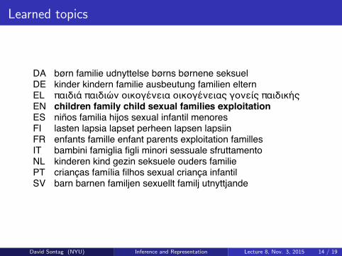
Figure 2 shows the most probable words in all lan-guages for four example topics, from PLTM with400 topics. The first topic contains words relatingto the European Central Bank. This topic providesan illustration of the variation in technical ter-minology captured by PLTM, including the widearray of acronyms used by different languages.The second topic, concerning children, demon-strates the variability of everyday terminology: al-though the four Romance languages are closely
882
David Sontag (NYU) Inference and Representation Lecture 8, Nov. 3, 2015 13 / 19
Learned topics
sampling. Gibbs sampling involves sequentiallyresampling each zl
n from its conditional posterior:
P (zln = t |w,z\l,n,�1, . . . ,�L,↵m)
/ �lwl
n|t(Nt)\l,n + ↵mtP
t Nt � 1 + ↵, (4)
where z\l,n is the current set of topic assignmentsfor all other tokens in the tuple, while (Nt)\l,n isthe number of occurrences of topic t in the tuple,excluding zl
n, the variable being resampled.
4 Results on Parallel Text
Our first set of experiments focuses on documenttuples that are known to consist of direct transla-tions. In this case, we can be confident that thetopic distribution is genuinely shared across alllanguages. Although direct translations in multi-ple languages are relatively rare (in contrast withcomparable documents), we use direct translationsto explore the characteristics of the model.
4.1 Data SetThe EuroParl corpus consists of parallel texts ineleven western European languages: Danish, Ger-man, Greek, English, Spanish, Finnish, French,Italian, Dutch, Portuguese and Swedish. Thesetexts consist of roughly a decade of proceedingsof the European parliament. For our purposes weuse alignments at the speech level rather than thesentence level, as in many translation tasks usingthis corpus. We also remove the twenty-five mostfrequent word types for efficiency reasons. Theremaining collection consists of over 121 millionwords. Details by language are shown in Table 1.
Table 1: Average document length, # documents, andunique word types per 10,000 tokens in the EuroParl corpus.
Lang. Avg. leng. # docs types/10kDA 160.153 65245 121.4DE 178.689 66497 124.5EL 171.289 46317 124.2EN 176.450 69522 43.1ES 170.536 65929 59.5FI 161.293 60822 336.2FR 186.742 67430 54.8IT 187.451 66035 69.5NL 176.114 66952 80.8PT 183.410 65718 68.2SV 154.605 58011 136.1
Models are trained using 1000 iterations ofGibbs sampling. Each language-specific topic–word concentration parameter �l is set to 0.01.
centralbank europæiske ecb s lån centralbanks zentralbank ezb bank europäischen investitionsbank darlehen τράπεζα τράπεζας κεντρική εκτ κεντρικής τράπεζες bank central ecb banks european monetary banco central europeo bce bancos centrales keskuspankin ekp n euroopan keskuspankki eip banque centrale bce européenne banques monétaire banca centrale bce europea banche prestiti bank centrale ecb europese banken leningen banco central europeu bce bancos empréstimos centralbanken europeiska ecb centralbankens s lån
børn familie udnyttelse børns børnene seksuel kinder kindern familie ausbeutung familien eltern παιδιά παιδιών οικογένεια οικογένειας γονείς παιδικής children family child sexual families exploitation niños familia hijos sexual infantil menores lasten lapsia lapset perheen lapsen lapsiin enfants famille enfant parents exploitation familles bambini famiglia figli minori sessuale sfruttamento kinderen kind gezin seksuele ouders familie crianças família filhos sexual criança infantil barn barnen familjen sexuellt familj utnyttjande
mål nå målsætninger målet målsætning opnå ziel ziele erreichen zielen erreicht zielsetzungen στόχους στόχο στόχος στόχων στόχοι επίτευξη objective objectives achieve aim ambitious set objetivo objetivos alcanzar conseguir lograr estos tavoite tavoitteet tavoitteena tavoitteiden tavoitteita tavoitteen objectif objectifs atteindre but cet ambitieux obiettivo obiettivi raggiungere degli scopo quello doelstellingen doel doelstelling bereiken bereikt doelen objectivo objectivos alcançar atingir ambicioso conseguir mål målet uppnå målen målsättningar målsättning
andre anden side ene andet øvrige anderen andere einen wie andererseits anderer άλλες άλλα άλλη άλλων άλλους όπως other one hand others another there otros otras otro otra parte demás muiden toisaalta muita muut muihin muun autres autre part côté ailleurs même altri altre altro altra dall parte andere anderzijds anderen ander als kant outros outras outro lado outra noutros andra sidan å annat ena annan
DADEELENESFIFRITNLPTSV DADEELENESFIFRITNLPTSV DADEELENESFIFRITNLPTSV DADEELENESFIFRITNLPTSV
Figure 2: EuroParl topics (T=400)
The concentration parameter ↵ for the prior overdocument-specific topic distributions is initializedto 0.01 T , while the base measure m is initializedto the uniform distribution. Hyperparameters ↵mare re-estimated every 10 Gibbs iterations.
4.2 Analysis of Trained Models
Figure 2 shows the most probable words in all lan-guages for four example topics, from PLTM with400 topics. The first topic contains words relatingto the European Central Bank. This topic providesan illustration of the variation in technical ter-minology captured by PLTM, including the widearray of acronyms used by different languages.The second topic, concerning children, demon-strates the variability of everyday terminology: al-though the four Romance languages are closely
882
David Sontag (NYU) Inference and Representation Lecture 8, Nov. 3, 2015 14 / 19
Discussion
How would you use this?
How could you extend this?
David Sontag (NYU) Inference and Representation Lecture 8, Nov. 3, 2015 15 / 19
Author-topic model (Rosen-Zvi et al., UAI ’04)
Goal: topic models that take into consideration author interests
Training data: corpora with label for who wrote each document
Papers from NIPS conference from 1987 to 1999Twitter posts from US politicians
Why do this?
How to do this?
David Sontag (NYU) Inference and Representation Lecture 8, Nov. 3, 2015 16 / 19
Author-topic model (Rosen-Zvi et al., UAI ’04)
z
wD
φβ
α θ
T
x
wNd D
φβA
dax
z
wD
φβ
α θA
T
da
(a)
Topic (LDA)
(b)
Author
(c)
Author-Topic
NdNd
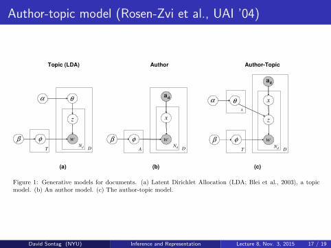
Figure 1: Generative models for documents. (a) Latent Dirichlet Allocation (LDA; Blei et al., 2003), a topicmodel. (b) An author model. (c) The author-topic model.
prior. The mixture weights corresponding to the cho-sen author are used to select a topic z, and a word isgenerated according to the distribution φ correspond-ing to that topic, drawn from a symmetric Dirichlet(β)prior.
The author-topic model subsumes the two models de-scribed above as special cases: topic models like LDAcorrespond to the case where each document has oneunique author, and the author model corresponds tothe case where each author has one unique topic. Byestimating the parameters φ and θ, we obtain informa-tion about which topics authors typically write about,as well as a representation of the content of each docu-ment in terms of these topics. In the remainder of thepaper, we will describe a simple algorithm for estimat-ing these parameters, compare these different models,and illustrate how the results produced by the author-topic model can be used to answer questions aboutwhich which authors work on similar topics.
3 Gibbs sampling algorithms
A variety of algorithms have been used to estimate theparameters of topic models, from basic expectation-maximization (EM; Hofmann, 1999), to approximateinference methods like variational EM (Blei et al.,2003), expectation propagation (Minka & Lafferty,2002), and Gibbs sampling (Griffiths & Steyvers,2004). Generic EM algorithms tend to face problemswith local maxima in these models (Blei et al., 2003),suggesting a move to approximate methods in whichsome of the parameters—such as φ and θ—can be in-tegrated out rather than explicitly estimated. In thispaper, we will use Gibbs sampling, as it provides a sim-ple method for obtaining parameter estimates underDirichlet priors and allows combination of estimates
from several local maxima of the posterior distribu-tion.
The LDA model has two sets of unknown parameters –the D document distributions θ, and the T topic distri-butions φ – as well as the latent variables correspond-ing to the assignments of individual words to topics z.By applying Gibbs sampling (see Gilks, Richardson, &Spiegelhalter, 1996), we construct a Markov chain thatconverges to the posterior distribution on z and thenuse the results to infer θ and φ (Griffiths & Steyvers,2004). The transition between successive states of theMarkov chain results from repeatedly drawing z fromits distribution conditioned on all other variables, sum-ming out θ and φ using standard Dirichlet integrals:
P (zi = j|wi = m, z−i,w−i) ∝CWT
mj + β!m′ CWT
m′j + V β
CDTdj + α
!j′ CDT
dj′ + Tα(1)
where zi = j represents the assignments of the ithword in a document to topic j , wi = m representsthe observation that the ith word is the mth word inthe lexicon, and z−i represents all topic assignmentsnot including the ith word. Furthermore, CWT
mj is thenumber of times word m is assigned to topic j, notincluding the current instance, and CDT
dj is the num-ber of times topic j has occurred in document d, notincluding the current instance. For any sample fromthis Markov chain, being an assignment of every wordto a topic, we can estimate φ and θ using
φmj =CWT
mj + β!m′ CWT
m′j + V β(2)
θdj =CDT
dj + α!
j′ CDTdj′ + Tα
(3)
David Sontag (NYU) Inference and Representation Lecture 8, Nov. 3, 2015 17 / 19
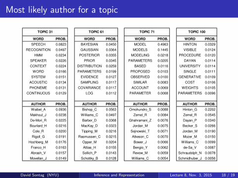
Most likely author for a topic
WORD PROB. WORD PROB. WORD PROB. WORD PROB.LIKELIHOOD 0.0539 RECOGNITION 0.0400 REINFORCEMENT 0.0411 KERNEL 0.0683
MIXTURE 0.0509 CHARACTER 0.0336 POLICY 0.0371 SUPPORT 0.0377EM 0.0470 CHARACTERS 0.0250 ACTION 0.0332 VECTOR 0.0257
DENSITY 0.0398 TANGENT 0.0241 OPTIMAL 0.0208 KERNELS 0.0217GAUSSIAN 0.0349 HANDWRITTEN 0.0169 ACTIONS 0.0208 SET 0.0205
ESTIMATION 0.0314 DIGITS 0.0159 FUNCTION 0.0178 SVM 0.0204LOG 0.0263 IMAGE 0.0157 REWARD 0.0165 SPACE 0.0188
MAXIMUM 0.0254 DISTANCE 0.0153 SUTTON 0.0164 MACHINES 0.0168PARAMETERS 0.0209 DIGIT 0.0149 AGENT 0.0136 REGRESSION 0.0155
ESTIMATE 0.0204 HAND 0.0126 DECISION 0.0118 MARGIN 0.0151
AUTHOR PROB. AUTHOR PROB. AUTHOR PROB. AUTHOR PROB.Tresp_V 0.0333 Simard_P 0.0694 Singh_S 0.1412 Smola_A 0.1033Singer_Y 0.0281 Martin_G 0.0394 Barto_A 0.0471 Scholkopf_B 0.0730Jebara_T 0.0207 LeCun_Y 0.0359 Sutton_R 0.0430 Burges_C 0.0489
Ghahramani_Z 0.0196 Denker_J 0.0278 Dayan_P 0.0324 Vapnik_V 0.0431Ueda_N 0.0170 Henderson_D 0.0256 Parr_R 0.0314 Chapelle_O 0.0210
Jordan_M 0.0150 Revow_M 0.0229 Dietterich_T 0.0231 Cristianini_N 0.0185Roweis_S 0.0123 Platt_J 0.0226 Tsitsiklis_J 0.0194 Ratsch_G 0.0172
Schuster_M 0.0104 Keeler_J 0.0192 Randlov_J 0.0167 Laskov_P 0.0169Xu_L 0.0098 Rashid_M 0.0182 Bradtke_S 0.0161 Tipping_M 0.0153
Saul_L 0.0094 Sackinger_E 0.0132 Schwartz_A 0.0142 Sollich_P 0.0141
WORD PROB. WORD PROB. WORD PROB. WORD PROB.SPEECH 0.0823 BAYESIAN 0.0450 MODEL 0.4963 HINTON 0.0329
RECOGNITION 0.0497 GAUSSIAN 0.0364 MODELS 0.1445 VISIBLE 0.0124HMM 0.0234 POSTERIOR 0.0355 MODELING 0.0218 PROCEDURE 0.0120
SPEAKER 0.0226 PRIOR 0.0345 PARAMETERS 0.0205 DAYAN 0.0114CONTEXT 0.0224 DISTRIBUTION 0.0259 BASED 0.0116 UNIVERSITY 0.0114
WORD 0.0166 PARAMETERS 0.0199 PROPOSED 0.0103 SINGLE 0.0111SYSTEM 0.0151 EVIDENCE 0.0127 OBSERVED 0.0100 GENERATIVE 0.0109
ACOUSTIC 0.0134 SAMPLING 0.0117 SIMILAR 0.0083 COST 0.0106PHONEME 0.0131 COVARIANCE 0.0117 ACCOUNT 0.0069 WEIGHTS 0.0105
CONTINUOUS 0.0129 LOG 0.0112 PARAMETER 0.0068 PARAMETERS 0.0096
AUTHOR PROB. AUTHOR PROB. AUTHOR PROB. AUTHOR PROB.Waibel_A 0.0936 Bishop_C 0.0563 Omohundro_S 0.0088 Hinton_G 0.2202Makhoul_J 0.0238 Williams_C 0.0497 Zemel_R 0.0084 Zemel_R 0.0545De-Mori_R 0.0225 Barber_D 0.0368 Ghahramani_Z 0.0076 Dayan_P 0.0340Bourlard_H 0.0216 MacKay_D 0.0323 Jordan_M 0.0075 Becker_S 0.0266
Cole_R 0.0200 Tipping_M 0.0216 Sejnowski_T 0.0071 Jordan_M 0.0190Rigoll_G 0.0191 Rasmussen_C 0.0215 Atkeson_C 0.0070 Mozer_M 0.0150
Hochberg_M 0.0176 Opper_M 0.0204 Bower_J 0.0066 Williams_C 0.0099Franco_H 0.0163 Attias_H 0.0155 Bengio_Y 0.0062 de-Sa_V 0.0087Abrash_V 0.0157 Sollich_P 0.0143 Revow_M 0.0059 Schraudolph_N 0.0078Movellan_J 0.0149 Schottky_B 0.0128 Williams_C 0.0054 Schmidhuber_J 0.0056
TOPIC 31 TOPIC 61 TOPIC 71 TOPIC 100
TOPIC 19 TOPIC 24 TOPIC 29 TOPIC 87
Figure 2: An illustration of 8 topics from a 100-topicsolution for the NIPS collection. Each topic is shownwith the 10 words and authors that have the highestprobability conditioned on that topic.
For each topic, the top 10 most likely authors are well-known authors in terms of NIPS papers written onthese topics (e.g., Singh, Barto, and Sutton in rein-forcement learning). While most (order of 80 to 90%)of the 100 topics in the model are similarly specificin terms of semantic content, the remaining 2 topicswe display illustrate some of the other types of “top-ics” discovered by the model. Topic 71 is somewhatgeneric, covering a broad set of terms typical to NIPSpapers, with a somewhat flatter distribution over au-thors compared to other topics. Topic 100 is somewhatoriented towards Geoff Hinton’s group at the Univer-sity of Toronto, containing the words that commonlyappeared in NIPS papers authored by members of thatresearch group, with an author list largely consistingof Hinton plus his past students and postdocs.
Figure 3 shows similar types of results for 4 selectedtopics from the CiteSeer data set, where again top-ics on speech recognition and Bayesian learning showup. However, since CiteSeer is much broader in con-tent (covering computer science in general) comparedto NIPS, it also includes a large number of topics not
WORD PROB. WORD PROB. WORD PROB. WORD PROB.SPEECH 0.1134 PROBABILISTIC 0.0778 USER 0.2541 STARS 0.0164
RECOGNITION 0.0349 BAYESIAN 0.0671 INTERFACE 0.1080 OBSERVATIONS 0.0150WORD 0.0295 PROBABILITY 0.0532 USERS 0.0788 SOLAR 0.0150
SPEAKER 0.0227 CARLO 0.0309 INTERFACES 0.0433 MAGNETIC 0.0145ACOUSTIC 0.0205 MONTE 0.0308 GRAPHICAL 0.0392 RAY 0.0144
RATE 0.0134 DISTRIBUTION 0.0257 INTERACTIVE 0.0354 EMISSION 0.0134SPOKEN 0.0132 INFERENCE 0.0253 INTERACTION 0.0261 GALAXIES 0.0124SOUND 0.0127 PROBABILITIES 0.0253 VISUAL 0.0203 OBSERVED 0.0108
TRAINING 0.0104 CONDITIONAL 0.0229 DISPLAY 0.0128 SUBJECT 0.0101MUSIC 0.0102 PRIOR 0.0219 MANIPULATION 0.0099 STAR 0.0087
AUTHOR PROB. AUTHOR PROB. AUTHOR PROB. AUTHOR PROB.Waibel_A 0.0156 Friedman_N 0.0094 Shneiderman_B 0.0060 Linsky_J 0.0143Gauvain_J 0.0133 Heckerman_D 0.0067 Rauterberg_M 0.0031 Falcke_H 0.0131Lamel_L 0.0128 Ghahramani_Z 0.0062 Lavana_H 0.0024 Mursula_K 0.0089
Woodland_P 0.0124 Koller_D 0.0062 Pentland_A 0.0021 Butler_R 0.0083Ney_H 0.0080 Jordan_M 0.0059 Myers_B 0.0021 Bjorkman_K 0.0078
Hansen_J 0.0078 Neal_R 0.0055 Minas_M 0.0021 Knapp_G 0.0067Renals_S 0.0072 Raftery_A 0.0054 Burnett_M 0.0021 Kundu_M 0.0063Noth_E 0.0071 Lukasiewicz_T 0.0053 Winiwarter_W 0.0020 Christensen-J 0.0059Boves_L 0.0070 Halpern_J 0.0052 Chang_S 0.0019 Cranmer_S 0.0055Young_S 0.0069 Muller_P 0.0048 Korvemaker_B 0.0019 Nagar_N 0.0050
TOPIC 10 TOPIC 209 TOPIC 87 TOPIC 20
Figure 3: An illustration of 4 topics from a 300-topicsolution for the CiteSeer collection. Each topic isshown with the 10 words and authors that have thehighest probability conditioned on that topic.
seen in NIPS, from user interfaces to solar astrophysics(Figure 3). Again the author lists are quite sensible—for example, Ben Shneiderman is a widely-known se-nior figure in the area of user-interfaces.
For the NIPS data set, 2000 iterations of the Gibbssampler took 12 hours of wall-clock time on a stan-dard PC workstation (22 seconds per iteration). Cite-seer took 111 hours for 700 iterations (9.5 minutesper iteration). The full list of tables can be foundat http://www.datalab.uci.edu/author-topic, forboth the 100-topic NIPS model and the 300-topic Cite-Seer model. In addition there is an online JAVAbrowser for interactively exploring authors, topics, anddocuments.
The results above use a single sample from the Gibbssampler. Across different samples each sample cancontain somewhat different topics i.e., somewhat dif-ferent sets of most probable words and authors giventhe topic, since according to the author-topic modelthere is not a single set of conditional probabilities, θand φ, but rather a distribution over these conditionalprobabilities. In the experiments in the sections below,we average over multiple samples (restricted to 10 forcomputational convenience) in a Bayesian fashion forpredictive purposes.
4.2 Evaluating predictive power
In addition to the qualitative evaluation of topic-author and topic-word results shown above, we alsoevaluated the proposed author-topic model in termsof perplexity, i.e., its ability to predict words on newunseen documents. We divided the D = 1, 740 NIPSpapers into a training set of 1, 557 papers with a totalof 2, 057, 729 words, and a test set of 183 papers of
David Sontag (NYU) Inference and Representation Lecture 8, Nov. 3, 2015 18 / 19
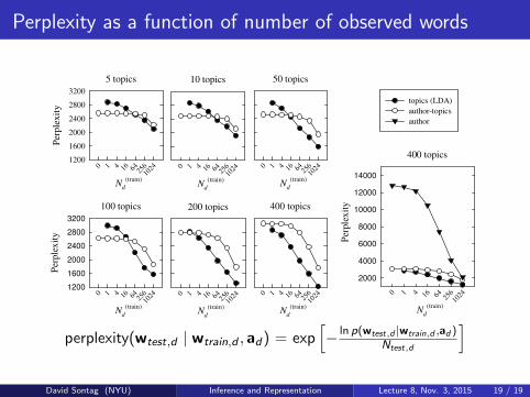
Perplexity as a function of number of observed words
5 topics
Nd(train)
0 1 4 16 64 25610
24
Perp
lexi
ty
1200
1600
2000
2400
2800
320010 topics
Nd(train)
0 1 4 16 64 25610
24
50 topics
Nd(train)
0 1 4 16 64 25610
24
100 topics
Nd(train)
0 1 4 16 64 25610
24
Perp
lexi
ty
1200
1600
2000
2400
2800
3200200 topics
Nd(train)
0 1 4 16 64 25610
24
400 topics
Nd(train)
0 1 4 16 64 25610
24
400 topics
Nd(train)
0 1 4 16 64 256
1024
Perp
lexi
ty
2000
4000
6000
8000
10000
12000
14000
topics (LDA)author-topicsauthor
Figure 4: Perplexity versus N(train)d for different numbers of topics, for the author, author-topic, and topic (LDA)
models.
ure 5 (thick line). We also derived the perplexity ofthe test documents conditioned on each one of the au-thors from the NIPS collection, perplexity(wd|a) fora = 1, ...,K. This results in K = 2, 037 different per-plexity values. Then we ranked the results and variouspercentiles from this ranking are presented in Figure5. One can see that making use of the authorshipinformation significantly improves the predictive log-likelihood: the model has accurate expectations aboutthe content of documents by particular authors. Asthe number of topics increases the ranking of the cor-rect author improves, where for 400 topics the aver-aged ranking of the correct author is within the 20highest ranked authors (out of 2,037 possible authors).Consequently, the model provides a useful method foridentifying possible authors for novel documents.
4.3 Illustrative applications of the model
The author-topic model could be used for a variety ofapplications such as automated reviewer recommenda-tions, i.e., given an abstract of a paper and a list of theauthors plus their known past collaborators, generatea list of other highly likely authors for this abstractwho might serve as good reviewers. Such a task re-quires computing the similarity between authors. Toillustrate how the model could be used in this respect,we defined the distance between authors i and j as thesymmetric KL divergence between the topics distribu-tion conditioned on each of the authors:
sKL(i, j) =
T!
t=1
"θit log
θit
θjt+ θjt log
θjt
θit
#. (9)
As earlier, we derived the averaged symmetric KL di-vergence by averaging over samples from the posterior
Table 1: Symmetric KL divergence for pairs of authors
Authors n T=400 T=200 T=100
Bartlett P (8) - 2.52 1.58 0.90Shawe-Taylor J (8)
Barto A (11) 2 3.34 2.18 1.25Singh S (17)Amari S (9) 3 3.44 2.48 1.57Yang H (5)
Singh S (17) 2 3.69 2.33 1.35Sutton R (7)
Moore A (11) - 4.25 2.89 1.87Sutton R (7)
MEDIAN - 5.52 4.01 3.33MAXIMUM - 16.61 14.91 13.32
Note: n is number of common papers in NIPS dataset.
distribution, p(θ|Dtrain).
We searched for similar pairs of authors in the NIPSdata set using the distance measure above. Wesearched only over authors who wrote more than 5papers in the full NIPS data set—there are 125 suchauthors out of the full set of 2037. Table 1 shows the5 pairs of authors with the highest averaged sKL forthe 400-topic model, as well as the median and min-imum. Results for the 200 and 100-topic models arealso shown as are the number of papers in the data setfor each author (in parentheses) and the number ofco-authored papers in the data set (2nd column). Allresults were averaged over 10 samples from the Gibbssampler.
Again the results are quite intuitive. For example,although authors Bartlett and Shawe-Taylor did nothave any co-authored documents in the NIPS collec-
perplexity(wtest,d | wtrain,d , ad) = exp[− ln p(wtest,d |wtrain,d ,ad )
Ntest,d
]
David Sontag (NYU) Inference and Representation Lecture 8, Nov. 3, 2015 19 / 19