Embed Size (px)
Citation preview
Method-of-moments
Daniel Hsu
1
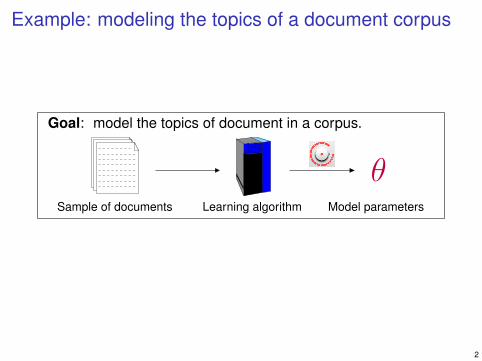
Example: modeling the topics of a document corpus
Goal: model the topics of document in a corpus.
Model parametersLearning algorithmSample of documents
θ
2
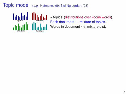
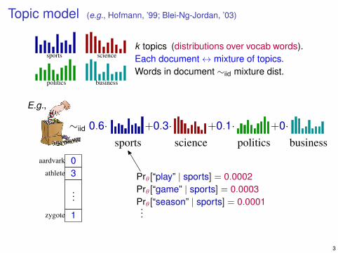
Topic model (e.g., Hofmann, ’99; Blei-Ng-Jordan, ’03)
sports science
businesspolitics
k topics (distributions over vocab words).Each document↔ mixture of topics.Words in document ∼iid mixture dist.
athlete
aardvark
zygote
sports science politics business
1
03
...
+0·∼iid 0.6· +0.3· +0.1·
E.g.,
Prθ[“play” | sports] = 0.0002Prθ[“game” | sports] = 0.0003Prθ[“season” | sports] = 0.0001...
3
Learning topic models
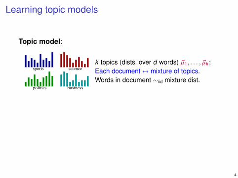
Topic model:
sports science
businesspolitics
k topics (dists. over d words) ~µ1, . . . , ~µk ;Each document↔ mixture of topics.Words in document ∼iid mixture dist.
I Input: sample of documents, generated by simple topicmodel with unknown parameters θ? := (~µt
?,wt?).
I Task: find parameters θ := (~µt ,wt ) so that θ ≈ θ?.
4
Learning topic models
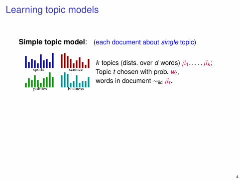
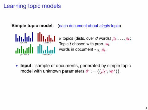
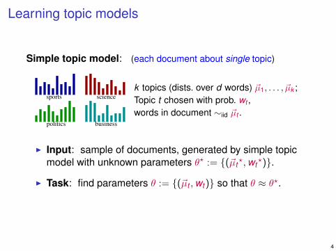
Simple topic model: (each document about single topic)
sports science
businesspolitics
k topics (dists. over d words) ~µ1, . . . , ~µk ;Topic t chosen with prob. wt ,words in document ∼iid ~µt .
I Input: sample of documents, generated by simple topicmodel with unknown parameters θ? := (~µt
?,wt?).
I Task: find parameters θ := (~µt ,wt ) so that θ ≈ θ?.
4
Learning topic models
Simple topic model: (each document about single topic)
sports science
businesspolitics
k topics (dists. over d words) ~µ1, . . . , ~µk ;Topic t chosen with prob. wt ,words in document ∼iid ~µt .
I Input: sample of documents, generated by simple topicmodel with unknown parameters θ? := (~µt
?,wt?).
I Task: find parameters θ := (~µt ,wt ) so that θ ≈ θ?.
4

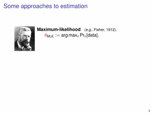
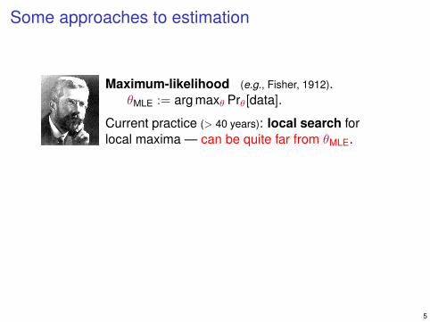
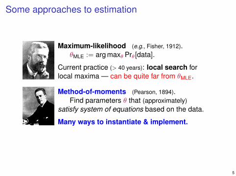
Some approaches to estimation
Maximum-likelihood (e.g., Fisher, 1912).θMLE := arg maxθ Prθ[data].
Current practice (> 40 years): local search forlocal maxima — can be quite far from θMLE.
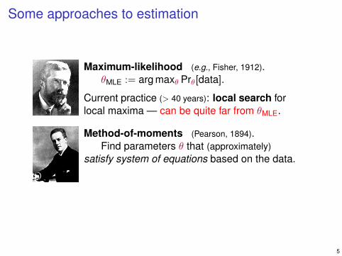
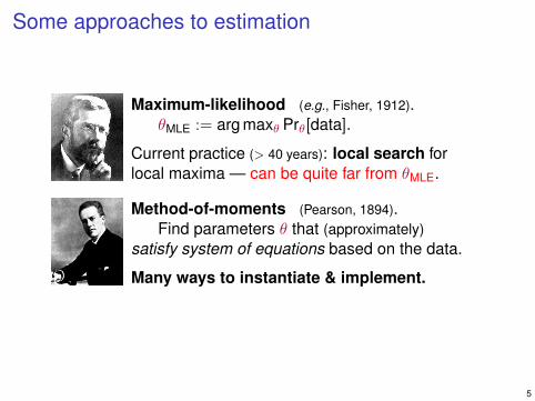
Method-of-moments (Pearson, 1894).Find parameters θ that (approximately)
satisfy system of equations based on the data.
Many ways to instantiate & implement.
5
Some approaches to estimation
Maximum-likelihood (e.g., Fisher, 1912).θMLE := arg maxθ Prθ[data].
Current practice (> 40 years): local search forlocal maxima — can be quite far from θMLE.
Method-of-moments (Pearson, 1894).Find parameters θ that (approximately)
satisfy system of equations based on the data.
Many ways to instantiate & implement.
5
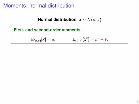
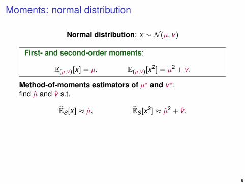
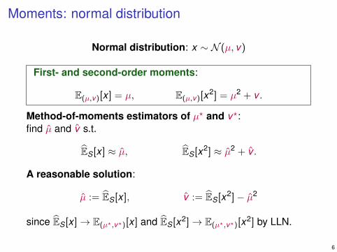
Moments: normal distribution
Normal distribution: x ∼ N (µ, v)
First- and second-order moments:
E(µ,v)[x ] = µ, E(µ,v)[x2] = µ2 + v .
Method-of-moments estimators of µ? and v?:find µ and v s.t.
ES[x ] ≈ µ, ES[x2] ≈ µ2 + v .
A reasonable solution:
µ := ES[x ], v := ES[x2]− µ2
since ES[x ]→ E(µ?,v?)[x ] and ES[x2]→ E(µ?,v?)[x2] by LLN.
6
Moments: simple topic model
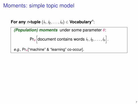
For any n-tuple (i1, i2, . . . , in) ∈ Vocabularyn:
(Population) moments under some parameter θ:
Prθ[document contains words i1, i2, . . . , in
].
e.g., Prθ[“machine” & “learning” co-occur].
Empirical moments from sample S of documents:
PrS
[document contains words i1, i2, . . . , in
]i.e., empirical frequency of co-occurrences in sample S.
7
Moments: simple topic model
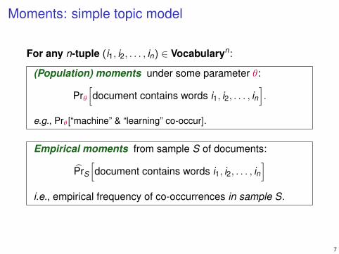
For any n-tuple (i1, i2, . . . , in) ∈ Vocabularyn:
(Population) moments under some parameter θ:
Prθ[document contains words i1, i2, . . . , in
].
e.g., Prθ[“machine” & “learning” co-occur].
Empirical moments from sample S of documents:
PrS
[document contains words i1, i2, . . . , in
]i.e., empirical frequency of co-occurrences in sample S.
7
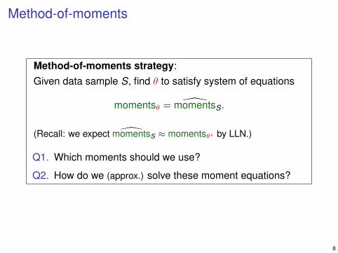
Method-of-moments
Method-of-moments strategy:Given data sample S, find θ to satisfy system of equations
momentsθ = momentsS.
(Recall: we expect momentsS ≈ momentsθ? by LLN.)
Q1. Which moments should we use?
Q2. How do we (approx.) solve these moment equations?
8

Q1. Which moments should we use?
9
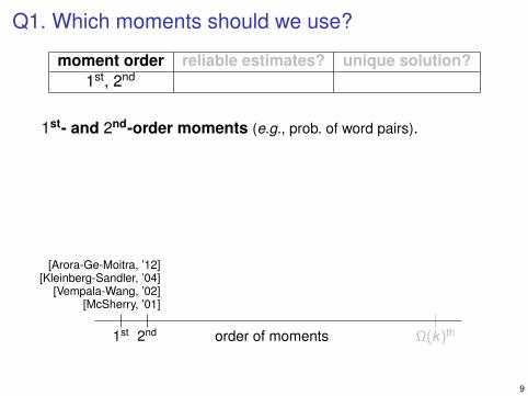
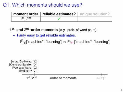
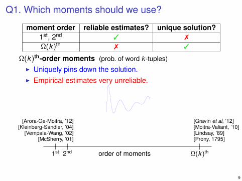
Q1. Which moments should we use?
moment order reliable estimates? unique solution?1st, 2nd
1st- and 2nd-order moments (e.g., prob. of word pairs).
[Vempala-Wang, ’02]
1st 2nd Ω(k)th
[McSherry, ’01]
order of moments
[Arora-Ge-Moitra, ’12][Kleinberg-Sandler, ’04]
9
Q1. Which moments should we use?
moment order reliable estimates? unique solution?1st, 2nd 3
1st- and 2nd-order moments (e.g., prob. of word pairs).I Fairly easy to get reliable estimates.
PrS[“machine”, “learning”] ≈ Prθ? [“machine”, “learning”]
[Vempala-Wang, ’02]
1st 2nd Ω(k)th
[McSherry, ’01]
order of moments
[Arora-Ge-Moitra, ’12][Kleinberg-Sandler, ’04]
9
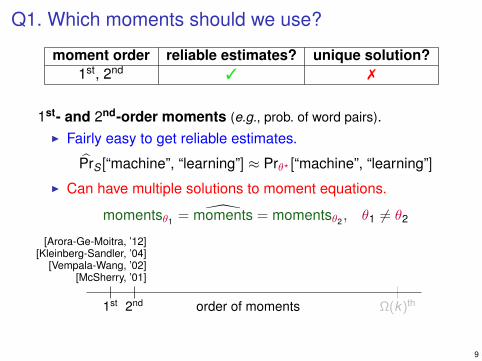
Q1. Which moments should we use?
moment order reliable estimates? unique solution?1st, 2nd 3 7
1st- and 2nd-order moments (e.g., prob. of word pairs).I Fairly easy to get reliable estimates.
PrS[“machine”, “learning”] ≈ Prθ? [“machine”, “learning”]
I Can have multiple solutions to moment equations.
momentsθ1 = moments = momentsθ2 , θ1 6= θ2
[Vempala-Wang, ’02]
1st 2nd Ω(k)th
[McSherry, ’01]
order of moments
[Arora-Ge-Moitra, ’12][Kleinberg-Sandler, ’04]
9
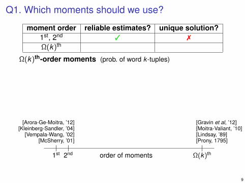
Q1. Which moments should we use?
moment order reliable estimates? unique solution?1st, 2nd 3 7
Ω(k)th
Ω(k)th-order moments (prob. of word k -tuples)
[Moitra-Valiant, ’10]
1st 2nd Ω(k)th
[McSherry, ’01] [Prony, 1795][Lindsay, ’89]
order of moments
[Arora-Ge-Moitra, ’12][Kleinberg-Sandler, ’04]
[Vempala-Wang, ’02]
[Gravin et al, ’12]
9
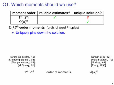
Q1. Which moments should we use?
moment order reliable estimates? unique solution?1st, 2nd 3 7
Ω(k)th 3
Ω(k)th-order moments (prob. of word k -tuples)I Uniquely pins down the solution.
[Moitra-Valiant, ’10]
1st 2nd Ω(k)th
[McSherry, ’01] [Prony, 1795][Lindsay, ’89]
order of moments
[Arora-Ge-Moitra, ’12][Kleinberg-Sandler, ’04]
[Vempala-Wang, ’02]
[Gravin et al, ’12]
9
Q1. Which moments should we use?
moment order reliable estimates? unique solution?1st, 2nd 3 7
Ω(k)th 7 3
Ω(k)th-order moments (prob. of word k -tuples)I Uniquely pins down the solution.I Empirical estimates very unreliable.
[Moitra-Valiant, ’10]
1st 2nd Ω(k)th
[McSherry, ’01] [Prony, 1795][Lindsay, ’89]
order of moments
[Arora-Ge-Moitra, ’12][Kleinberg-Sandler, ’04]
[Vempala-Wang, ’02]
[Gravin et al, ’12]
9
Q1. Which moments should we use?
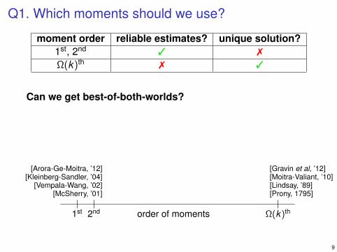
moment order reliable estimates? unique solution?1st, 2nd 3 7
Ω(k)th 7 3
Can we get best-of-both-worlds?
[Moitra-Valiant, ’10]
1st 2nd Ω(k)th
[McSherry, ’01] [Prony, 1795][Lindsay, ’89]
order of moments
[Arora-Ge-Moitra, ’12][Kleinberg-Sandler, ’04]
[Vempala-Wang, ’02]
[Gravin et al, ’12]
9
Q1. Which moments should we use?
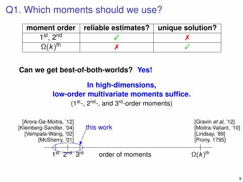
moment order reliable estimates? unique solution?1st, 2nd 3 7
Ω(k)th 7 3
Can we get best-of-both-worlds? Yes!
In high-dimensions,low-order multivariate moments suffice.
(1st-, 2nd-, and 3rd-order moments)
[Vempala-Wang, ’02]
1st 2nd Ω(k)th
[McSherry, ’01] [Prony, 1795][Lindsay, ’89]
3rd order of moments
this work [Moitra-Valiant, ’10][Gravin et al, ’12][Arora-Ge-Moitra, ’12]
[Kleinberg-Sandler, ’04]
9
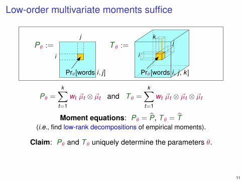
Low-order multivariate moments suffice
Key observation: in high dimensions (d k ),low-order moments have simple (“low-rank”) algebraic structure.
10

Low-order multivariate moments suffice
j
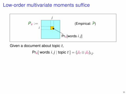
i(Empirical: P)Pθ :=
Prθ[words i , j]
Given a document about topic t ,
Prθ[ words i , j | topic t ] = (~µt )i · (~µt )j .
Claim: Pθ and T θ uniquely determine the parameters θ.
11
Low-order multivariate moments suffice
j
i(Empirical: P)Pθ :=
Prθ[words i , j]
Given a document about topic t ,
Prθ[ words i , j | topic t ] = (~µt ⊗ ~µt )i,j .
Claim: Pθ and T θ uniquely determine the parameters θ.
11
Low-order multivariate moments suffice
j
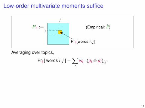
i(Empirical: P)Pθ :=
Prθ[words i , j]
Averaging over topics,
Prθ[ words i , j ] =∑
t
wt · (~µt ⊗ ~µt )i,j .
Claim: Pθ and T θ uniquely determine the parameters θ.
11
Low-order multivariate moments suffice
j
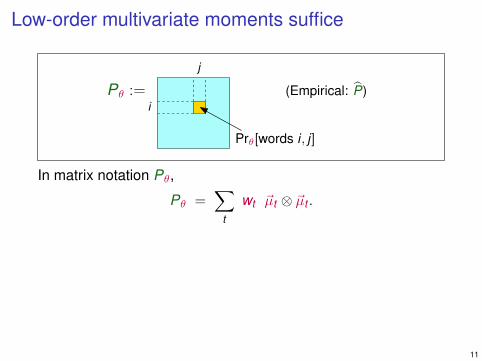
i(Empirical: P)Pθ :=
Prθ[words i , j]
In matrix notation Pθ,
Pθ =∑
t
wt ~µt ⊗ ~µt .
Claim: Pθ and T θ uniquely determine the parameters θ.
11
Low-order multivariate moments suffice
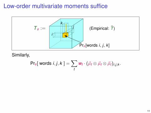
(Empirical: T )T θ :=i
jk
Prθ[words i , j , k ]
Similarly,
Prθ[ words i , j , k ] =∑
t
wt · (~µt ⊗ ~µt ⊗ ~µt )i,j,k .
Claim: Pθ and T θ uniquely determine the parameters θ.
11
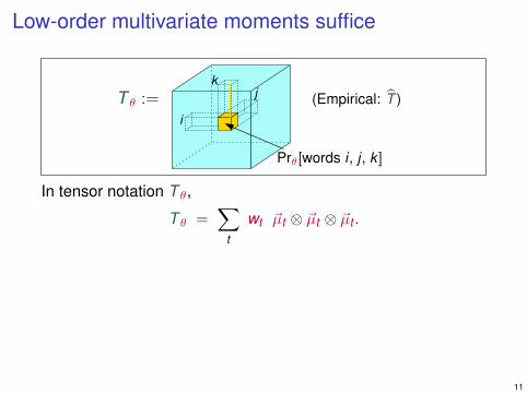
Low-order multivariate moments suffice
(Empirical: T )T θ :=i
jk
Prθ[words i , j , k ]
In tensor notation T θ,
T θ =∑
t
wt ~µt ⊗ ~µt ⊗ ~µt .
Claim: Pθ and T θ uniquely determine the parameters θ.
11
Low-order multivariate moments suffice
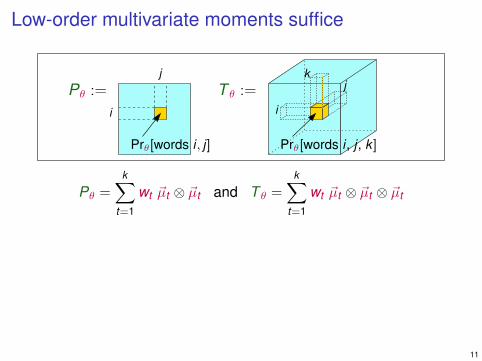
j
i
T θ :=Pθ :=i
jk
Prθ[words i , j , k ]Prθ[words i , j]
Pθ =k∑
t=1
wt ~µt ⊗ ~µt and T θ =k∑
t=1
wt ~µt ⊗ ~µt ⊗ ~µt
Claim: Pθ and T θ uniquely determine the parameters θ.
11
Low-order multivariate moments suffice
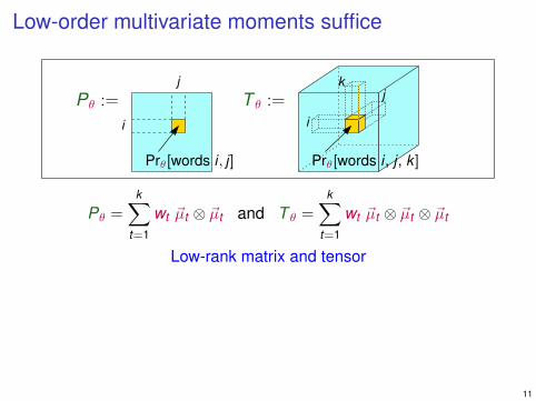
j
i
T θ :=Pθ :=i
jk
Prθ[words i , j , k ]Prθ[words i , j]
Pθ =k∑
t=1
wt ~µt ⊗ ~µt and T θ =k∑
t=1
wt ~µt ⊗ ~µt ⊗ ~µt
Low-rank matrix and tensor
Claim: Pθ and T θ uniquely determine the parameters θ.
11
Low-order multivariate moments suffice
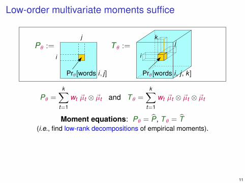
j
i
T θ :=Pθ :=i
jk
Prθ[words i , j , k ]Prθ[words i , j]
Pθ =k∑
t=1
wt ~µt ⊗ ~µt and T θ =k∑
t=1
wt ~µt ⊗ ~µt ⊗ ~µt
Moment equations: Pθ = P, T θ = T(i.e., find low-rank decompositions of empirical moments).
Claim: Pθ and T θ uniquely determine the parameters θ.
11
Low-order multivariate moments suffice
j
i
T θ :=Pθ :=i
jk
Prθ[words i , j , k ]Prθ[words i , j]
Pθ =k∑
t=1
wt ~µt ⊗ ~µt and T θ =k∑
t=1
wt ~µt ⊗ ~µt ⊗ ~µt
Moment equations: Pθ = P, T θ = T(i.e., find low-rank decompositions of empirical moments).
Claim: Pθ and T θ uniquely determine the parameters θ.
11
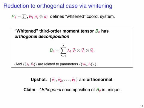
Reduction to orthogonal case via whitening
Pθ =∑
t wt ~µt ⊗ ~µt defines “whitened” coord. system.
Upshot: ~v1, ~v2, . . . , ~vk are orthonormal.
Claim: Orthogonal decomposition of Bθ is unique.
12
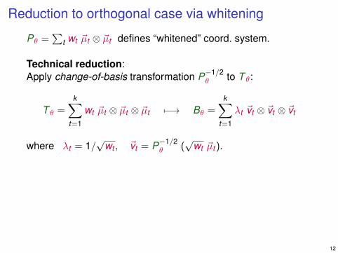
Reduction to orthogonal case via whitening
Pθ =∑
t wt ~µt ⊗ ~µt defines “whitened” coord. system.
Technical reduction:Apply change-of-basis transformation P−1/2
θ to T θ:
T θ =k∑
t=1
wt ~µt ⊗ ~µt ⊗ ~µt 7−→ Bθ =k∑
t=1
λt ~vt ⊗ ~vt ⊗ ~vt
where λt = 1/√
wt , ~vt = P−1/2θ (
√wt ~µt ).
Upshot: ~v1, ~v2, . . . , ~vk are orthonormal.
Claim: Orthogonal decomposition of Bθ is unique.
12
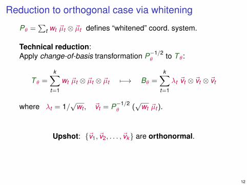
Reduction to orthogonal case via whitening
Pθ =∑
t wt ~µt ⊗ ~µt defines “whitened” coord. system.
Technical reduction:Apply change-of-basis transformation P−1/2
θ to T θ:
T θ =k∑
t=1
wt ~µt ⊗ ~µt ⊗ ~µt 7−→ Bθ =k∑
t=1
λt ~vt ⊗ ~vt ⊗ ~vt
where λt = 1/√
wt , ~vt = P−1/2θ (
√wt ~µt ).
Upshot: ~v1, ~v2, . . . , ~vk are orthonormal.
Claim: Orthogonal decomposition of Bθ is unique.
12
Reduction to orthogonal case via whitening
Pθ =∑
t wt ~µt ⊗ ~µt defines “whitened” coord. system.
“Whitened” third-order moment tensor Bθ hasorthogonal decomposition
Bθ =k∑
t=1
λt ~vt ⊗ ~vt ⊗ ~vt .
(And (λt , ~vt) are related to parameters (wt , ~µt).)
Upshot: ~v1, ~v2, . . . , ~vk are orthonormal.
Claim: Orthogonal decomposition of Bθ is unique.
12
The spectral theorem and eigendecompositions
13
The spectral theorem and eigendecompositions
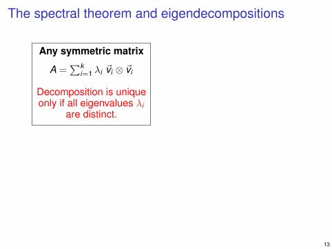
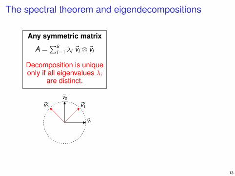
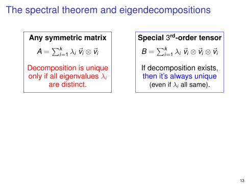
Any symmetric matrix
Decomposition is unique
are distinct.only if all eigenvalues λi
A =∑k
i=1 λi ~vi ⊗ ~vi
13

The spectral theorem and eigendecompositions
Any symmetric matrix
Decomposition is unique
are distinct.only if all eigenvalues λi
A =∑k
i=1 λi ~vi ⊗ ~vi
~v2
~v1
13
The spectral theorem and eigendecompositions
Any symmetric matrix
Decomposition is unique
are distinct.only if all eigenvalues λi
A =∑k
i=1 λi ~vi ⊗ ~vi
~v2
~v ′1~v ′
2
~v1
13
The spectral theorem and eigendecompositions
Any symmetric matrix
Decomposition is unique
are distinct.only if all eigenvalues λi
A =∑k
i=1 λi ~vi ⊗ ~vi
Special 3rd-order tensor
B =∑k
i=1 λi ~vi ⊗ ~vi ⊗ ~vi
If decomposition exists,
(even if λi all same).then it’s always unique
13
The spectral theorem and eigendecompositions
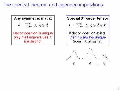
Any symmetric matrix
Decomposition is unique
are distinct.only if all eigenvalues λi
A =∑k
i=1 λi ~vi ⊗ ~vi
Special 3rd-order tensor
B =∑k
i=1 λi ~vi ⊗ ~vi ⊗ ~vi
If decomposition exists,
(even if λi all same).then it’s always unique
· · ·~v2~v1 ~vk
13
The spectral theorem and eigendecompositions
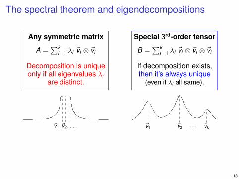
Any symmetric matrix
Decomposition is unique
are distinct.only if all eigenvalues λi
A =∑k
i=1 λi ~vi ⊗ ~vi
Special 3rd-order tensor
B =∑k
i=1 λi ~vi ⊗ ~vi ⊗ ~vi
If decomposition exists,
(even if λi all same).then it’s always unique
~v1, ~v2, . . . · · ·~v2~v1 ~vk
13

The spectral theorem and eigendecompositions
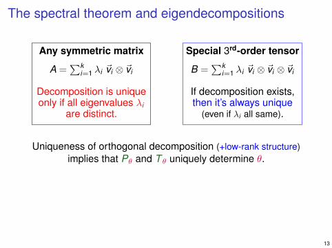
Any symmetric matrix
Decomposition is unique
are distinct.only if all eigenvalues λi
A =∑k
i=1 λi ~vi ⊗ ~vi
Special 3rd-order tensor
B =∑k
i=1 λi ~vi ⊗ ~vi ⊗ ~vi
If decomposition exists,
(even if λi all same).then it’s always unique
Uniqueness of orthogonal decomposition (+low-rank structure)implies that Pθ and T θ uniquely determine θ.
13
The spectral theorem and eigendecompositions
Any symmetric matrix
Decomposition is unique
are distinct.only if all eigenvalues λi
A =∑k
i=1 λi ~vi ⊗ ~vi
Special 3rd-order tensor
B =∑k
i=1 λi ~vi ⊗ ~vi ⊗ ~vi
If decomposition exists,
(even if λi all same).then it’s always unique
Uniqueness of orthogonal decomposition (+low-rank structure)implies that Pθ and T θ uniquely determine θ.
13

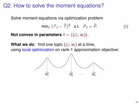
Q2. How to solve the moment equations?
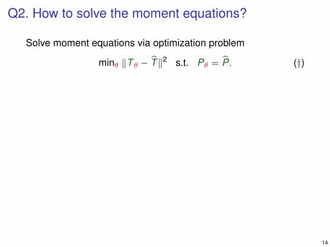
Solve moment equations via optimization problem
minθ ‖T θ − T‖2 s.t. Pθ = P. (†)
Not convex in parameters θ = (~µi ,wi).
What we do: find one topic (~µi ,wi) at a time,using local optimization on rank-1 approximation objective:
Can approximate all local optima, each corresp. to a topic.−→ Near-optimal solution to (†).
14
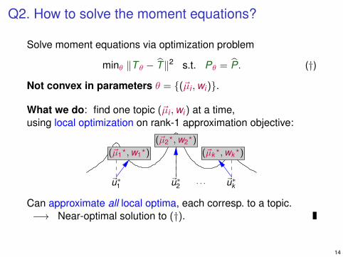
Q2. How to solve the moment equations?
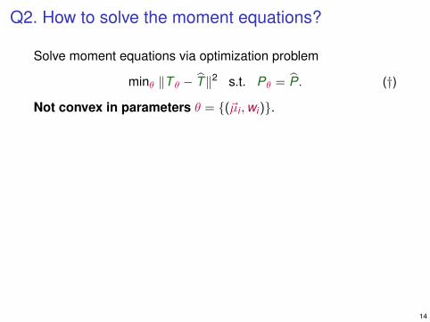
Solve moment equations via optimization problem
minθ ‖T θ − T‖2 s.t. Pθ = P. (†)
Not convex in parameters θ = (~µi ,wi).
What we do: find one topic (~µi ,wi) at a time,using local optimization on rank-1 approximation objective:
Can approximate all local optima, each corresp. to a topic.−→ Near-optimal solution to (†).
14
Q2. How to solve the moment equations?
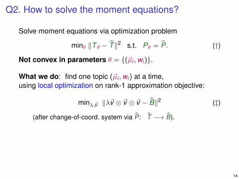
Solve moment equations via optimization problem
minθ ‖T θ − T‖2 s.t. Pθ = P. (†)
Not convex in parameters θ = (~µi ,wi).
What we do: find one topic (~µi ,wi) at a time,using local optimization on rank-1 approximation objective:
minλ,~v ‖λ~v ⊗ ~v ⊗ ~v − B‖2 (‡)
(after change-of-coord. system via P: T −→ B).
Can approximate all local optima, each corresp. to a topic.−→ Near-optimal solution to (†).
14
Q2. How to solve the moment equations?
Solve moment equations via optimization problem
minθ ‖T θ − T‖2 s.t. Pθ = P. (†)
Not convex in parameters θ = (~µi ,wi).
What we do: find one topic (~µi ,wi) at a time,using local optimization on rank-1 approximation objective:
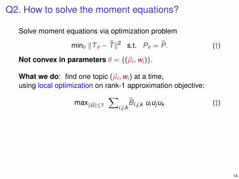
max‖~u‖≤1
∑i,j,k
Bi,j,k uiujuk (‡)
Can approximate all local optima, each corresp. to a topic.−→ Near-optimal solution to (†).
14
Q2. How to solve the moment equations?
Solve moment equations via optimization problem
minθ ‖T θ − T‖2 s.t. Pθ = P. (†)
Not convex in parameters θ = (~µi ,wi).
What we do: find one topic (~µi ,wi) at a time,using local optimization on rank-1 approximation objective:
· · ·~u∗1 ~u∗
2 ~u∗k
Can approximate all local optima, each corresp. to a topic.−→ Near-optimal solution to (†).
14
Q2. How to solve the moment equations?
Solve moment equations via optimization problem
minθ ‖T θ − T‖2 s.t. Pθ = P. (†)
Not convex in parameters θ = (~µi ,wi).
What we do: find one topic (~µi ,wi) at a time,using local optimization on rank-1 approximation objective:
~u∗k~u∗
1 · · ·~u∗2
(~µk?,wk
?)(~µ1?,w1
?)
(~µ2?,w2
?)
Can approximate all local optima, each corresp. to a topic.−→ Near-optimal solution to (†).
14
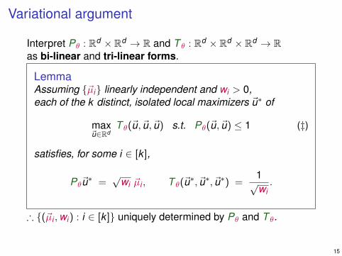
Variational argument
Interpret Pθ : Rd × Rd → R and T θ : Rd × Rd × Rd → Ras bi-linear and tri-linear forms.
LemmaAssuming ~µi linearly independent and wi > 0,each of the k distinct, isolated local maximizers ~u∗ of
max~u∈Rd
T θ(~u, ~u, ~u) s.t. Pθ(~u, ~u) ≤ 1 (‡)
satisfies, for some i ∈ [k ],
Pθ~u∗ =√
wi ~µi , T θ(~u∗, ~u∗, ~u∗) =1√wi.
∴ (~µi ,wi) : i ∈ [k ] uniquely determined by Pθ and T θ.
15
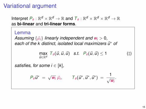
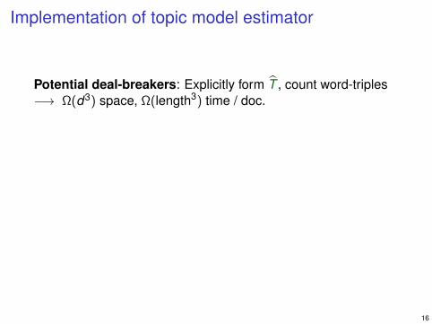
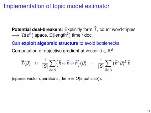
Implementation of topic model estimator
Potential deal-breakers: Explicitly form T , count word-triples−→ Ω(d3) space, Ω(length3) time / doc.
Can exploit algebraic structure to avoid bottlenecks.
16
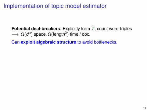
Implementation of topic model estimator
Potential deal-breakers: Explicitly form T , count word-triples−→ Ω(d3) space, Ω(length3) time / doc.
Can exploit algebraic structure to avoid bottlenecks.
16
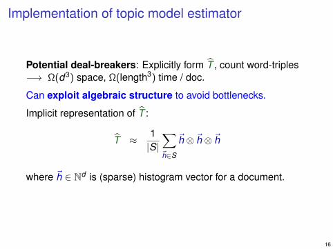
Implementation of topic model estimator
Potential deal-breakers: Explicitly form T , count word-triples−→ Ω(d3) space, Ω(length3) time / doc.
Can exploit algebraic structure to avoid bottlenecks.
Implicit representation of T :
T ≈ 1|S|∑~h∈S
~h ⊗ ~h ⊗ ~h
where ~h ∈ Nd is (sparse) histogram vector for a document.
16
Implementation of topic model estimator
Potential deal-breakers: Explicitly form T , count word-triples−→ Ω(d3) space, Ω(length3) time / doc.
Can exploit algebraic structure to avoid bottlenecks.
Computation of objective gradient at vector ~u ∈ Rd :
T (~u) ≈ 1|S|∑~h∈S
(~h ⊗ ~h ⊗ ~h
)(~u) =
1|S|∑~h∈S
(~h>~u)2 ~h
(sparse vector operations; time = O(input size)).
16
Illustrative empirical results
I Corpus: 300000 New York Times articles.I Vocabulary size: 102660 words.I Set number of topics k := 50.
Predictive performance of straightforward implementation:≈ 4–8× speed-up over Gibbs sampling.
0 0.5 1 1.5 2
8.4
8.6
Training time (×104 sec)
Log
loss
Method-of-momentsGibbs sampling
17
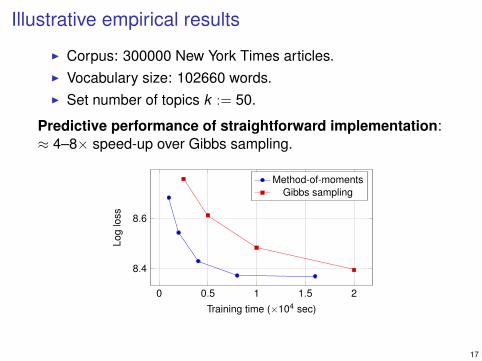
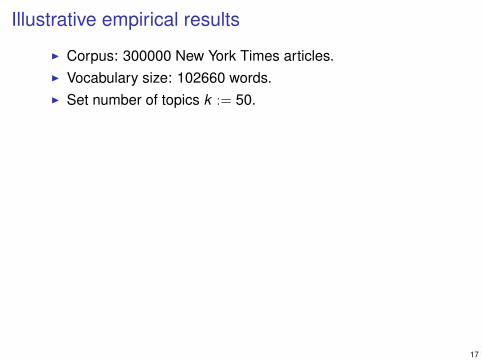

Illustrative empirical results
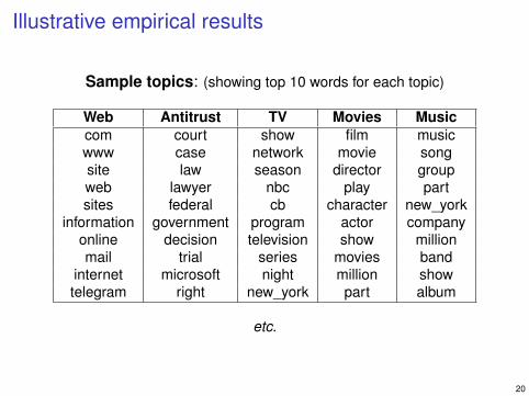
Sample topics: (showing top 10 words for each topic)
Econ. Baseball Edu. Health care Golfsales run school drug player
economic inning student patient tiger_woodconsumer hit teacher million won
major game program company shothome season official doctor play
indicator home public companies roundweekly right children percent winorder games high cost tournamentclaim dodger education program tour
scheduled left district health right
18
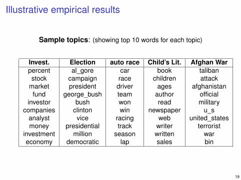
Illustrative empirical results
Sample topics: (showing top 10 words for each topic)
Invest. Election auto race Child’s Lit. Afghan Warpercent al_gore car book talibanstock campaign race children attack
market president driver ages afghanistanfund george_bush team author official
investor bush won read militarycompanies clinton win newspaper u_s
analyst vice racing web united_statesmoney presidential track writer terrorist
investment million season written wareconomy democratic lap sales bin
19
Illustrative empirical results
Sample topics: (showing top 10 words for each topic)
Web Antitrust TV Movies Musiccom court show film musicwww case network movie songsite law season director groupweb lawyer nbc play partsites federal cb character new_york
information government program actor companyonline decision television show millionmail trial series movies band
internet microsoft night million showtelegram right new_york part album
etc.
20
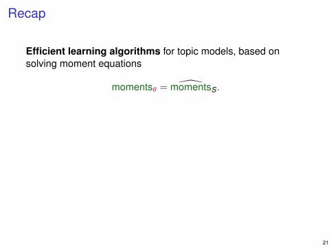
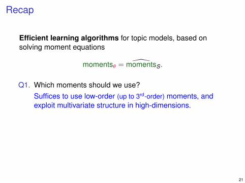
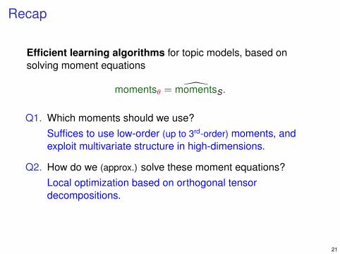
Recap
Efficient learning algorithms for topic models, based onsolving moment equations
momentsθ = momentsS.
Q1. Which moments should we use?Suffices to use low-order (up to 3rd-order) moments, andexploit multivariate structure in high-dimensions.
Q2. How do we (approx.) solve these moment equations?Local optimization based on orthogonal tensordecompositions.
21
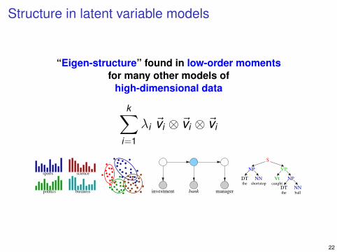
Structure in latent variable models
“Eigen-structure” found in low-order momentsfor many other models of
high-dimensional data
k∑i=1
λi ~vi ⊗ ~vi ⊗ ~vi
sports science
businesspolitics bank managerinvestment
NP
NP
DT NNshortstop
DT NNthe ball
Vtcaught
VP
S
the
22
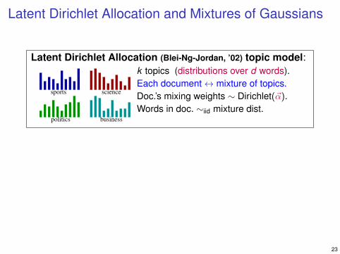
Latent Dirichlet Allocation and Mixtures of Gaussians
Latent Dirichlet Allocation (Blei-Ng-Jordan, ’02) topic model:
sports science
businesspolitics
k topics (distributions over d words).Each document↔ mixture of topics.Doc.’s mixing weights ∼ Dirichlet(~α).Words in doc. ∼iid mixture dist.
Mixtures of Gaussians (Pearson, 1894)
k sub-populations in Rd ;t-th sub-pop. modeled as Gaussian N (~µt , Σt )with mixing weight wt .
23
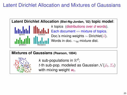
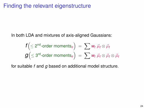
Finding the relevant eigenstructure
In both LDA and mixtures of axis-aligned Gaussians:
f(≤ 2nd-order momentsθ
)=∑
wt ~µt ⊗ ~µt
g(≤ 3rd-order momentsθ
)=∑
wt ~µt ⊗ ~µt ⊗ ~µt
for suitable f and g based on additional model structure.
24
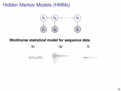
Hidden Markov Models (HMMs)
h1 h2 · · · h`
~x1 ~x2 ~x`
Workhorse statistical model for sequence data
/k/ /a/ /t/
I Hidden state variables h1 → h2 → · · · form a Markov chain.I Observation ~xt at time t depends only on hidden state ht at
time t .
25
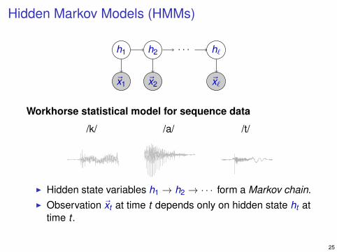
Hidden Markov Models (HMMs)
h1 h2 · · · h`
~x1 ~x2 ~x`
Workhorse statistical model for sequence data
/k/ /a/ /t/
I Hidden state variables h1 → h2 → · · · form a Markov chain.I Observation ~xt at time t depends only on hidden state ht at
time t .
25
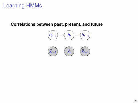
Learning HMMs
Correlations between past, present, and future
ht−1 ht ht+1
~xt−1 ~xt ~xt+1
Suffices to use low-order (asymmetric) cross moments
Eθ[ ~xt−1 ⊗ ~xt ⊗ ~xt+1 ].
26
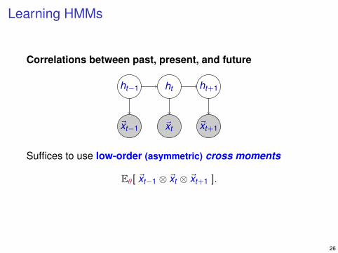
Learning HMMs
Correlations between past, present, and future
ht−1 ht ht+1
~xt−1 ~xt ~xt+1
Suffices to use low-order (asymmetric) cross moments
Eθ[ ~xt−1 ⊗ ~xt ⊗ ~xt+1 ].
26
Where to read more
Tensor decompositions for learning latent variable modelsA. Anandkumar, R. Ge, D. Hsu, S. M. Kakade, M. Telgarsky
Journal of Machine Learning Research, 2014.
http://jmlr.org/papers/v15/anandkumar14b.html
27


![Allahabad Magh Mela of 1894€¦ · March 1894.] ALLAHABAD MAGH MELA OP 1894. 97 ALLA.HA13AD MAGH MELA OF 1894. Eveiiy January a large gathering, partly religious and partly mercantile](https://img.pdfslide.us/doc/110x75/5fc01678b23b4859cd4726a9/allahabad-magh-mela-of-1894-march-1894-allahabad-magh-mela-op-1894-97-allaha13ad.jpg)


![Daisy 1894 Manual[1]](https://img.pdfslide.us/doc/110x75/5571f82749795991698cc2ee/daisy-1894-manual1.jpg)