In every way that matters, anything the mind imagines, exists. The existencestems either from an external idea perceived by the mind, or an internal notion

initiated by ones own creativity.

University of Alberta

Imperfect Channel Knowledge for Interference Avoidance

by

Saina Lajevardi

A thesis submitted to the Faculty of Graduate Studies and Research in partialfulfillment of the requirements for the degree of

Master of Sciencein

Communications

Department of Electrical and Computer Engineering

c© Saina LajevardiSpring 2011

Edmonton, Alberta

Permission is hereby granted to the University of Alberta Library to reproduce single copies ofthis thesis and to lend or sell such copies for private, scholarly or scientific research purposes only.Where the thesis is converted to, or otherwise made available in digital form, the University of

Alberta will advise potential users of the thesis of these terms.

The author reserves all other publication and other rights in association with the copyright in thethesis, and except as herein before provided, neither the thesis nor any substantial portion thereofmay be printed or otherwise reproduced in any material form whatever without the author’s prior

written permission.

University of Alberta

Faculty of Graduate Studies and Research

The undersigned certify that they have read, and recommend to the Faculty ofGraduate Studies and Research for acceptance, a thesis entitled Imperfect Chan-nel Knowledge for Interference Avoidance submitted by Saina Lajevardi inpartial fulfillment of the requirements for the degree of Master of Science.

Dr. Christian SchlegelSupervisor

Dr. Behrouz NowrouzianCo-Supervisor

Dr. Bruce F. Cockburn

Dr. Iannis NikolaidisExternal Examiner

Date:

To my mom, Mitra, who has always been the angel of my life.

Abstract

This thesis examines various signal processing techniques that are required for estab-

lishing efficient (near optimal) communications in multiuser multiple-input multiple-

output (MIMO) environments. The central part of this thesis is dedicated to ac-

quisition of information about the MIMO channel state - at both the receiver and

the transmitter. This information is required to organize a communication set up

which utilizes all the available channel resources. Realistic channel model, i.e., the

spatial channel model (SCM), has been used in this study, together with modern

long-term evolution (LTE) standard.

The work consists of three major themes: (a) estimation of the channel at the

receiver, also known as tracking; (b) quantization of the channel information and

its feedback from receiver to the transmitter (feedback quantization); and (c) recon-

struction of the channel knowledge at the transmitter, and its use for data precoding

during communication transmission.

Acknowledgements

It is a great pleasure for me to thank my supervisor, Dr. Christian Schlegel, for his

guidance throughout this work. I am specially obliged to Dr. Dmitry Trukhachev

for his endless care and patience; this thesis would have not be completed with-

out his help. I would like to thank my amazing friends: Mahdi Ramezani for his

helpful discussions on communications systems, as well as his expertise in LATEX;

Rasoul Milasi and Sahar Movaghati for their encouragement and research advice;

my old friends, Obilor Nawmadi and Mahdi Rahimi, for their support from far away

(through online chats and emails). I drew tremendous strength from members of my

family: from my mother, father, brother, and older sister, who live so far away, and

from my little sister, Parmida, and my wonderful friend and roommate, Reihaneh

Rabbany, who are with me in Edmonton.

I would like to acknowledge contributions from my colleagues, Marcel Jar, Majid

Ghanbarinezhad and Russel Dodd, who each in his own way had helped with the

completion of this work.

Friendship for me is the strength to keep working and to follow my dreams. Here,

I would like to acknowledge my great friends: Mahdi Ramezani, Dr. Mohammad

Behnam, Mohammad Mehdi Khajeh, Navid Paydavousi, and Farzaneh Saba, who

have always been supporting me in both good and bad times. Their unconditional

friendship was something I could always count on. Finally, I would like to thank my

best friend, Dr. Anthony Yeung, for his intellectual support and attention during

the last stages of my work. His support and friendship encouraged me to keep up

the hard work and to remain optimistic at all times.

Table of Contents

1 Introduction 11.1 Motivation . . . . . . . . . . . . . . . . . . . . . . . . . . . . . . . . 11.2 Wireless Communications with Multiple Antennas . . . . . . . . . . 21.3 Mobile Cellular Communications . . . . . . . . . . . . . . . . . . . . 31.4 Thesis Outline . . . . . . . . . . . . . . . . . . . . . . . . . . . . . . 5

2 Background 72.1 The Capacity of MIMO Channels . . . . . . . . . . . . . . . . . . . . 72.2 Beamforming . . . . . . . . . . . . . . . . . . . . . . . . . . . . . . . 8

2.2.1 beamforming with Multiple Users . . . . . . . . . . . . . . . . 92.2.2 Downlink Beamforming . . . . . . . . . . . . . . . . . . . . . 10

2.3 The Long-Term Evolution System (LTE) . . . . . . . . . . . . . . . 122.3.1 LTE Specifications . . . . . . . . . . . . . . . . . . . . . . . . 122.3.2 LTE Transmission Format . . . . . . . . . . . . . . . . . . . . 13

2.4 The Spatial Channel Model (SCM) . . . . . . . . . . . . . . . . . . . 15

3 Channel Estimation 193.1 The Estimation Problem . . . . . . . . . . . . . . . . . . . . . . . . . 193.2 Wiener Filter . . . . . . . . . . . . . . . . . . . . . . . . . . . . . . . 20

3.2.1 Principle of Orthogonality . . . . . . . . . . . . . . . . . . . . 213.3 Methods of Steepest Descent (SD) and LMS Algorithm . . . . . . . 23

3.3.1 The SD Algorithm . . . . . . . . . . . . . . . . . . . . . . . . 243.3.2 Stochastic Gradient-Based Algorithms: the LMS Approach . 25

3.4 Example: Channel Estimation in the MIMO Scenario . . . . . . . . 27

4 Channel State Information Feedback and Quantization 324.1 Finite-Rate Feedback of CSI . . . . . . . . . . . . . . . . . . . . . . . 324.2 Feedback Quantization for Multiuser MIMO, Problem Definition and

Approach . . . . . . . . . . . . . . . . . . . . . . . . . . . . . . . . . 344.3 Codebook Design . . . . . . . . . . . . . . . . . . . . . . . . . . . . . 37

4.3.1 Random Vector Quantization (RVQ) . . . . . . . . . . . . . . 384.3.2 Grassmannian Line(Subspace) Packing . . . . . . . . . . . . . 39

4.4 Experimental Results . . . . . . . . . . . . . . . . . . . . . . . . . . . 404.4.1 Joint Channel Estimation and Quantization Feedback . . . . 43

5 Limited Feedback in Time-Varying Multipath MIMO Channels 465.1 Multipath Channel Model . . . . . . . . . . . . . . . . . . . . . . . . 47

5.1.1 LTE Multipath Characteristics . . . . . . . . . . . . . . . . . 485.2 Channel Estimation in MIMO-OFDM . . . . . . . . . . . . . . . . . 49

5.2.1 Channel Estimation in LTE . . . . . . . . . . . . . . . . . . . 505.2.2 OFDM Structure in Terms of Estimation . . . . . . . . . . . 51

5.3 LTE Channel Reconstruction at Transmitter . . . . . . . . . . . . . 535.4 Feedback Schemes for Multipath MIMO Channels with LTE . . . . . 54

6 Concluding Remarks and Future Work 58

Bibliography 61

List of Figures

1.1 Basic communication system for MIMO channels. . . . . . . . . . . . 31.2 Illustration of the interference dominance in cellular networks. . . . . 41.3 Sampled target and interferer power distribution for the SCM. The

interferer is at distance 550m [1] – see Figure 1.2. . . . . . . . . . . . 5

2.1 Mathematical basics of beamforming. . . . . . . . . . . . . . . . . . . 92.2 Downlink beamforming using precoding separation among different

users. . . . . . . . . . . . . . . . . . . . . . . . . . . . . . . . . . . . 102.3 LTE resource block. . . . . . . . . . . . . . . . . . . . . . . . . . . . 112.4 LTE frame structure. . . . . . . . . . . . . . . . . . . . . . . . . . . . 132.5 BS and MS angular parameters [1]. . . . . . . . . . . . . . . . . . . . 15

3.1 Filtering system block diagram. . . . . . . . . . . . . . . . . . . . . . 203.2 Uplink transmission scenario. Two vehicles are approaching one an-

other, each at a speed of 60km/h. . . . . . . . . . . . . . . . . . . . . 273.3 LMS channel tracking for the reference transmitter. . . . . . . . . . 283.4 Autocorrelation function of the residual error of the LMS channel

estimation. . . . . . . . . . . . . . . . . . . . . . . . . . . . . . . . . 293.5 Projection loss for two passing transmitters. . . . . . . . . . . . . . . 303.6 Projection loss for two passing transmitters where the LMS is used

to estimate the interfering channel with samples taken every 1ms. . . 31

4.1 Capacity performance of Grassmannian and Random Vector Quanti-zation with 2 and 3 feedback-bit. . . . . . . . . . . . . . . . . . . . . 39

4.2 Capacity performance of Grassmannian and Random Vector Quanti-zation with a large number of bits. . . . . . . . . . . . . . . . . . . . 40

4.3 Capacity performance of Grassmannian and Random Vector Quanti-zation with a constant number of feedback bits. . . . . . . . . . . . . 41

4.4 LMS channel tracking of the power of the wireless channel from thefirst BS antenna to the MS. . . . . . . . . . . . . . . . . . . . . . . . 42

4.5 Autocorrelation function of the residual error. . . . . . . . . . . . . . 434.6 Capacity performance using different forms of CSIR and CSIT. . . . 44

5.1 ISI in OFDM system. . . . . . . . . . . . . . . . . . . . . . . . . . . 475.2 Multipath delay spread histogram in the macro urban scenario. . . . 495.3 Frequency response of the multipath in macro urban scenario-HSDP. 505.4 Frequency response of the multipath in macro urban scenario-LTE. . 515.5 LTE time-frequency resource grid with pilot locations. . . . . . . . . 52

5.6 SCM signal Reconstruction with Doppler rate and 8-bit feedback persample. . . . . . . . . . . . . . . . . . . . . . . . . . . . . . . . . . . 53

5.7 SCM signal Reconstruction sampled at 4 times Doppler rate with 2bits of feedback per sample. . . . . . . . . . . . . . . . . . . . . . . . 54

5.8 ZF capacity performance for LTE. . . . . . . . . . . . . . . . . . . . 57

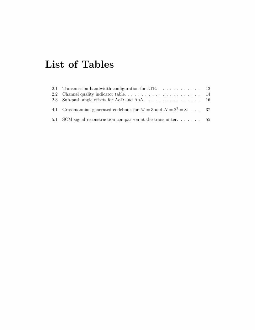
List of Tables

2.1 Transmission bandwidth configuration for LTE. . . . . . . . . . . . . 122.2 Channel quality indicator table. . . . . . . . . . . . . . . . . . . . . . 142.3 Sub-path angle offsets for AoD and AoA. . . . . . . . . . . . . . . . 16

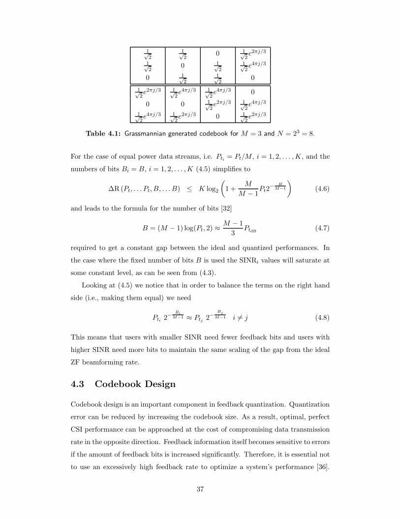
4.1 Grassmannian generated codebook for M = 3 and N = 23 = 8. . . . 37

5.1 SCM signal reconstruction comparison at the transmitter. . . . . . . 55

List of Symbols

Symbol Definition First Use

Am×n An m by n matrix . . . . . . . . . . . . . . . . . . . . . . . 2

η Gaussian noise . . . . . . . . . . . . . . . . . . . . . . . . . 2

a A vector . . . . . . . . . . . . . . . . . . . . . . . . . . . . . 3

τ Time delay . . . . . . . . . . . . . . . . . . . . . . . . . . . 3

Pt The transmit power . . . . . . . . . . . . . . . . . . . . . . 7

C The channel capacity . . . . . . . . . . . . . . . . . . . . . . 7

ρ The signal-to-noise ratio . . . . . . . . . . . . . . . . . . . . 7

H The channel matrix . . . . . . . . . . . . . . . . . . . . . . . 7

Q The covariance matrix . . . . . . . . . . . . . . . . . . . . . 7

tr(·) Trace of the enclosed matrix . . . . . . . . . . . . . . . . . . 7

det(.) Determinant of the enclosed matrix . . . . . . . . . . . . . . 7

I The identity matrix . . . . . . . . . . . . . . . . . . . . . . 7

N Number of receive antennas . . . . . . . . . . . . . . . . . . 7

E Expected value operator . . . . . . . . . . . . . . . . . . . . 8

(.) The complex conjugate . . . . . . . . . . . . . . . . . . . . . 8

|.| The vector Euclidean norm . . . . . . . . . . . . . . . . . . 8

(.)−1 The matrix inverse . . . . . . . . . . . . . . . . . . . . . . . 9

P The projection vector . . . . . . . . . . . . . . . . . . . . . 9

J Cost function for formulating Wiener filtering problem . . . 21

(.)H The conjugate transpose (Hermitian) . . . . . . . . . . . . . 24

p Cross-correlation vector . . . . . . . . . . . . . . . . . . . . 24

R Ensemble-average correlation matrix . . . . . . . . . . . . . 24

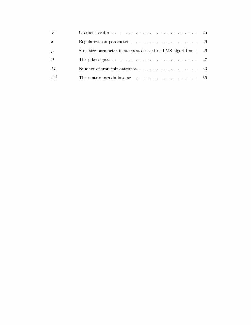
∇ Gradient vector . . . . . . . . . . . . . . . . . . . . . . . . . 25

δ Regularization parameter . . . . . . . . . . . . . . . . . . . 26

µ Step-size parameter in steepest-descent or LMS algorithm . 26

P The pilot signal . . . . . . . . . . . . . . . . . . . . . . . . . 27

M Number of transmit antennas . . . . . . . . . . . . . . . . . 33

(.)† The matrix pseudo-inverse . . . . . . . . . . . . . . . . . . . 35

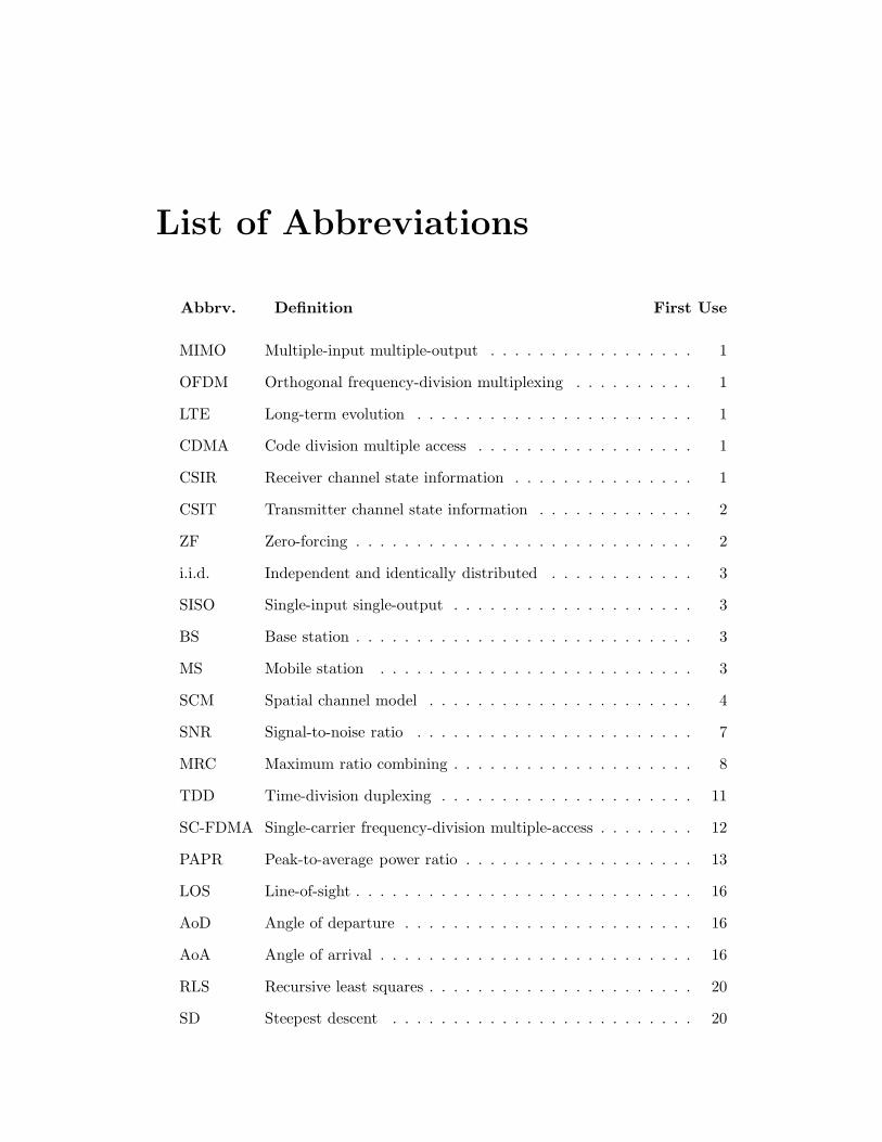
List of Abbreviations

Abbrv. Definition First Use

MIMO Multiple-input multiple-output . . . . . . . . . . . . . . . . . 1

OFDM Orthogonal frequency-division multiplexing . . . . . . . . . . 1

LTE Long-term evolution . . . . . . . . . . . . . . . . . . . . . . . 1

CDMA Code division multiple access . . . . . . . . . . . . . . . . . . 1

CSIR Receiver channel state information . . . . . . . . . . . . . . . 1

CSIT Transmitter channel state information . . . . . . . . . . . . . 2

ZF Zero-forcing . . . . . . . . . . . . . . . . . . . . . . . . . . . . 2

i.i.d. Independent and identically distributed . . . . . . . . . . . . 3

SISO Single-input single-output . . . . . . . . . . . . . . . . . . . . 3

BS Base station . . . . . . . . . . . . . . . . . . . . . . . . . . . . 3

MS Mobile station . . . . . . . . . . . . . . . . . . . . . . . . . . 3

SCM Spatial channel model . . . . . . . . . . . . . . . . . . . . . . 4

SNR Signal-to-noise ratio . . . . . . . . . . . . . . . . . . . . . . . 7

MRC Maximum ratio combining . . . . . . . . . . . . . . . . . . . . 8

TDD Time-division duplexing . . . . . . . . . . . . . . . . . . . . . 11

SC-FDMA Single-carrier frequency-division multiple-access . . . . . . . . 12

PAPR Peak-to-average power ratio . . . . . . . . . . . . . . . . . . . 13

LOS Line-of-sight . . . . . . . . . . . . . . . . . . . . . . . . . . . . 16

AoD Angle of departure . . . . . . . . . . . . . . . . . . . . . . . . 16

AoA Angle of arrival . . . . . . . . . . . . . . . . . . . . . . . . . . 16

RLS Recursive least squares . . . . . . . . . . . . . . . . . . . . . . 20

SD Steepest descent . . . . . . . . . . . . . . . . . . . . . . . . . 20

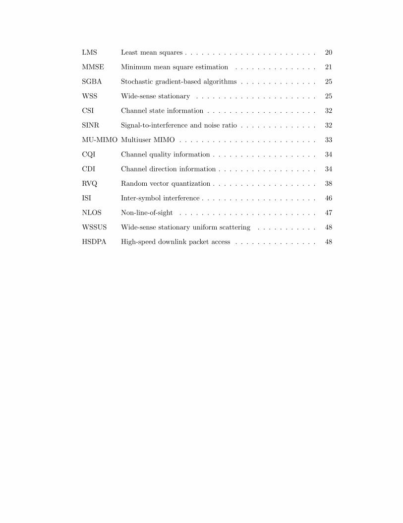
LMS Least mean squares . . . . . . . . . . . . . . . . . . . . . . . . 20

MMSE Minimum mean square estimation . . . . . . . . . . . . . . . 21

SGBA Stochastic gradient-based algorithms . . . . . . . . . . . . . . 25

WSS Wide-sense stationary . . . . . . . . . . . . . . . . . . . . . . 25

CSI Channel state information . . . . . . . . . . . . . . . . . . . . 32

SINR Signal-to-interference and noise ratio . . . . . . . . . . . . . . 32

MU-MIMO Multiuser MIMO . . . . . . . . . . . . . . . . . . . . . . . . . 33

CQI Channel quality information . . . . . . . . . . . . . . . . . . . 34

CDI Channel direction information . . . . . . . . . . . . . . . . . . 34

RVQ Random vector quantization . . . . . . . . . . . . . . . . . . . 38

ISI Inter-symbol interference . . . . . . . . . . . . . . . . . . . . . 46

NLOS Non-line-of-sight . . . . . . . . . . . . . . . . . . . . . . . . . 47

WSSUS Wide-sense stationary uniform scattering . . . . . . . . . . . 48

HSDPA High-speed downlink packet access . . . . . . . . . . . . . . . 48

Chapter 1

Introduction

1.1 Motivation

The enormous demands for high data rate and quality of service mobile communi-

cation systems are the basis for the deployment of new technologies for future of

wireless communications. Multiple-input multiple-output (MIMO) and orthogonal

frequency-division multiplexing (OFDM) are two such techniques which are suitable

for upcoming cellular networks requirements. MIMO and OFDM are utilized as the

underlying technologies for standards such as IEEE 802.11n, WiMAX, and 3GPP

long-term evolution (LTE).

The emerging needs for increasingly higher data rate telecommunication intro-

duce many new challenges into the transmission systems. LTE is the most recent

standard introduced by the International Telecommunications Union (ITU) which

satisfies the anticipated users’ requirements, with a large number of new techno-

logical and architectural features, including OFDM as the air interface instead of

wideband Code division multiple access (CDMA) as in third generation mobile (3G)

systems. However, LTE is not yet a 4G technology as it does not accomplish all the

requirements set forth for 4G [2]. For this reason, it has sometimes been referred to

as the 3.99G of cellular networks.

Some of the specifications of LTE make it a pioneer in capacity improvement and

interference mitigation, which is the main motivation of this thesis. Larger network

coverage, higher quality services and faster transmission rates all lead to interference

throughout the network. A thorough knowledge of the channel is critical to avoiding

interference by the different transmission techniques. The acquisition of channel

state information at the receiver (CSIR) is done by adaptive channel estimation

techniques. Providing the transmitter with this knowledge will bring up another set

1

of challenges to the system which is typically addressed by feedback. Utilizing the

channel information at the transmitter (CSIT), the transmitter applies precoding

techniques to reduce interference over the entire system. This will be discussed

further throughout this thesis. In this thesis, the zero-forcing (ZF) capacity with

perfect channel knowledge is determined as the system’s upper bound on achievable

performance. Also, we limit the multiuser MIMO system to either two users or

single-antenna mobile terminals.

1.2 Wireless Communications with Multiple Antennas

MIMO is a key technology to enabling high data rate transmission in wireless com-

munications; see Section 1.1. High data rate transmissions on the order of a giga-byte

seems feasible with MIMO transmission technology [3]. One can regard MIMO as an

extension of smart antenna [4]. The objective of a smart antenna is to concentrate

all the transmitted energy to the point of interest. In essence, MIMO transmits data

in all channel matrix dimensions with no additional power and bandwidth. Thus,

the benefits of MIMO go beyond the smart antenna concept.

MIMO has been the main vehicle in mobile wireless communications for several

years now. The studies of Alamouti and Tarokh introduced a new dimension to the

field of MIMO known as space-time coding [5, 6]. According to [7], MIMO studies

can be classified into three main fields: information and coding theory, channel

modeling and adaptive signal processing, and antenna arrays.

Priliminary Concepts

The composite MIMO channel with a matrix HN×M (τ, t) consists of N receive

antennas and M transmit antennas; see Fig. 1.1. The discrete-time input-output

relation for signal transmission over a single carrier is given by

y =

√

Ec

MHc+ η

where c is the transmitted signal, and Ec is the total transmitted power.

The received signal yj(t) at the jth antenna is given by

yj(t) =

M∑

i=1

hji(τ, t)ci(t) + ηj(t), (1.1)

2

Received

Baseband Signals

Baseband Signals

Parallel RF Stages

Parallel RF Stages

Figure 1.1: Basic communication system for MIMO channels.

where ηj(t) is Gaussian receiver noise, and the path strength hji(τ , t) describes the

time variation and frequency selectivity of the channel from the ith transmit antenna

to the jth receive antenna.

MIMO results in an additional dimension which is known as the spatial dimen-

sion. The exact architecture for spatial multiplexing is given in [8, 9]. Spatial mul-

tiplexing gain improves the spectral efficiency of the channel with no requirement

for additional power and bandwidth, where different data streams are transmitted

over different antennas and received independently. From an information theoretic

point of view, the amount of information that a transmission system is capable of

carrying is given by the Shannon capacity [10], which is further discussed in the

following section.

The original papers on MIMO capacity model the channel matrix elements ide-

ally as independent and identically distributed (i.i.d.) Gaussian random variables

which correspond to a very rich scattering environment. Different measurements of

real MIMO environments have been performed in [11–13], for example. The mea-

surements confirm the capacity improvement of MIMO compared to the traditional

single-input single-output (SISO) system in urban and suburban environments. The

indoor environment, however, benefits from rich multipath scattering which leads

to higher spectral efficiencies.

1.3 Mobile Cellular Communications

Every cellular networks consists of a number of cells being virtually partitioned,

including a base station (BS) transceiver and number of users, known as mobile sta-

tions (MS). The concept behind the partitioning is to reuse the frequency resources

to serve an unlimited number of users; see Fig. 1.2. There are, however, several

transmission issues in the cellular networks:

3

Area of

High

Interference

Area of lowInterference

Interfering BS

Main BS

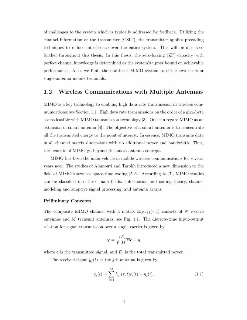
Figure 1.2: Illustration of the interference dominance in cellular networks.

1. The variety of radio transmission channels resulting from large user coverage

and the shape of the cellular networks. This diversity originates from a number

of reasons – such as mobility of the MS’s, multipath effects, different channel

paths, and random signal phase arrivals which introduce position-dependant

fading to the phase and location of the radio signals.

2. The presence of interference in two forms: inter-cell interference and intra-

cell interference. Intra-cell interference is technically avoided in LTE system

due to channel orthogonalization. In contrast, inter-cell interference, which is

interference at the cell edges, is much harder to avoid. A number of solutions,

such as cell interference coordinations, have been proposed for LTE systems.

These solutions, however, are still far from being implemented [14].

Cellular Systems: Interference

In practice, most cellular networks are interference-limited [15]. In cellular networks,

a large number of MSs are subjected to strong levels of interference; see Fig. 1.2.

Assuming the distribution of the users is normal, the majority of them will be close

to edges and using possibly the same resources. In the analytical approach, user

interference is typically regarded as white Gaussian noise for the sake of simplicity.

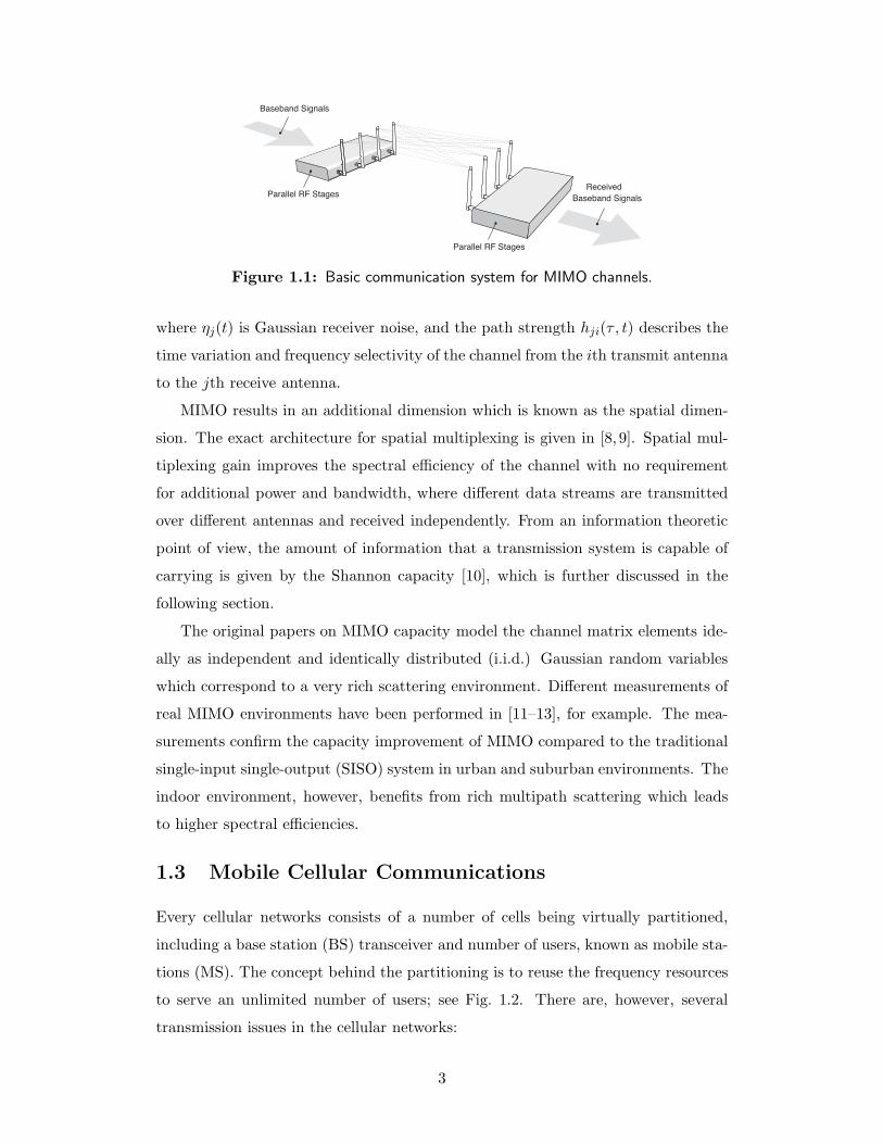
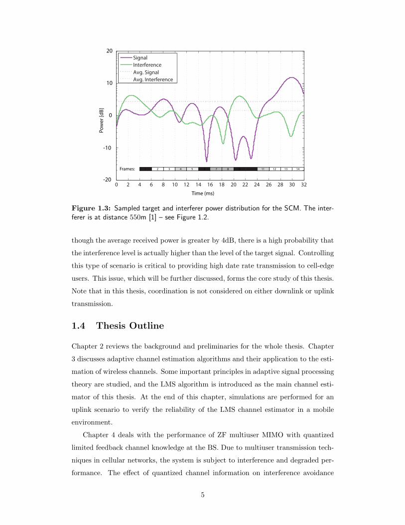
Fig. 1.3 shows the signal strength of a target user (purple) in comparison to the

signal of an interference from a neighboring cell (green). The target MS is at 450m

from the central BS, and 550m from the BS in the neighboring cell. The spatial

channel model (SCM) was used to generate these samples; see Section 2.4. Even

4

0 2 4 6 8 10 12 14 16 18 20 22 24 26 28 30 32

Signal

Interference

Avg. Signal

Avg. Interference

20

10

0

-10

-20

Frames: 1 2 3 4 5 6 7 8 9 10 11 12 13 14

Time (ms)

Po

we

r [d

B]

Figure 1.3: Sampled target and interferer power distribution for the SCM. The inter-ferer is at distance 550m [1] – see Figure 1.2.

though the average received power is greater by 4dB, there is a high probability that

the interference level is actually higher than the level of the target signal. Controlling

this type of scenario is critical to providing high date rate transmission to cell-edge

users. This issue, which will be further discussed, forms the core study of this thesis.

Note that in this thesis, coordination is not considered on either downlink or uplink

transmission.

1.4 Thesis Outline

Chapter 2 reviews the background and preliminaries for the whole thesis. Chapter

3 discusses adaptive channel estimation algorithms and their application to the esti-

mation of wireless channels. Some important principles in adaptive signal processing

theory are studied, and the LMS algorithm is introduced as the main channel esti-

mator of this thesis. At the end of this chapter, simulations are performed for an

uplink scenario to verify the reliability of the LMS channel estimator in a mobile

environment.

Chapter 4 deals with the performance of ZF multiuser MIMO with quantized

limited feedback channel knowledge at the BS. Due to multiuser transmission tech-

niques in cellular networks, the system is subject to interference and degraded per-

formance. The effect of quantized channel information on interference avoidance

5

forms the core of this chapter. At the end of this chapter, the ZF performance is

evaluated in the context of estimation and feedback errors. Chapter 5 is devoted to

the similar concepts of interference avoidance, data precoding and limited feedback,

but applied here to a more challenging transmission environment. Multipath in LTE

is the channel environment of interest, and the effects of feedback of both frequency

and time domain information are analyzed. Chapter 6 summarizes the key points

of this thesis and addresses some possible future directions.

6

Chapter 2

Background

2.1 The Capacity of MIMO Channels

The amount of information which can be transmitted reliably over a channel with

negligible probability of error is measured by the channel capacity. The channel

capacity is basically defined by the mutual information between the input and the

output signal [10]. However, proper transmission schemes are required to attain the

maximum channel capacity.

Channel Capacity for Single-User System

The channel capacity of a SISO system with a transmit power constraint Pt and

constant channel is given by

C = log(1 + ρ) bits/sec/Hz,

where ρ is the signal-to-noise ratio (SNR) of the receiver.

In practice, the channel gains change due to the multipath environment and the

fading effects of wireless communications. Therefore, the ergodic (mean) capacity

or average mutual information is [16]

C = EH

{log2

(1 + ρ‖H‖2

)}

Channel Capacity for the System with Multiple Antennas

The capacity for a constant channel that is known at both end of the multiple

antenna system is given by

C = maxQ:tr(Q)=Pt

log[

det(

IN +HQH†)]

where Q is the input covariance matrix [17].

7

Similarly, the ergodic capacity of the MIMO system with a flat fading channel,

Gaussian noise distribution and perfect CSIT and CSIR is given by

C = EH

{

maxQ:tr(Q)=Pt

log[

det(

IN +HQH†)]}

.

This capacity is maximized by optimizing the transmit power covariance matrix

[16,17]. This occurs when Pt is distributed equally among all transmit antennas,i.e.

when the covariance matrix is identity:

C = maxQ:tr(Q)=Pt

C(Q)

where

C(Q) ∼= EH

{

log[

det(

IN +HQH†)]}

Therefore, when the covariance matrix Q is optimized, the ergodic capacity is

C = EH

{

log

[

det

(

IN +Pt

MHH†

)]}

The expectation is taken over the distribution of the random channel matrix H.

2.2 Beamforming

Beamforming is widely used in wireless communications, radar, sonar, speech, and

biomedicine. Adaptive beamforming is used to detect the signal-of-interest at the

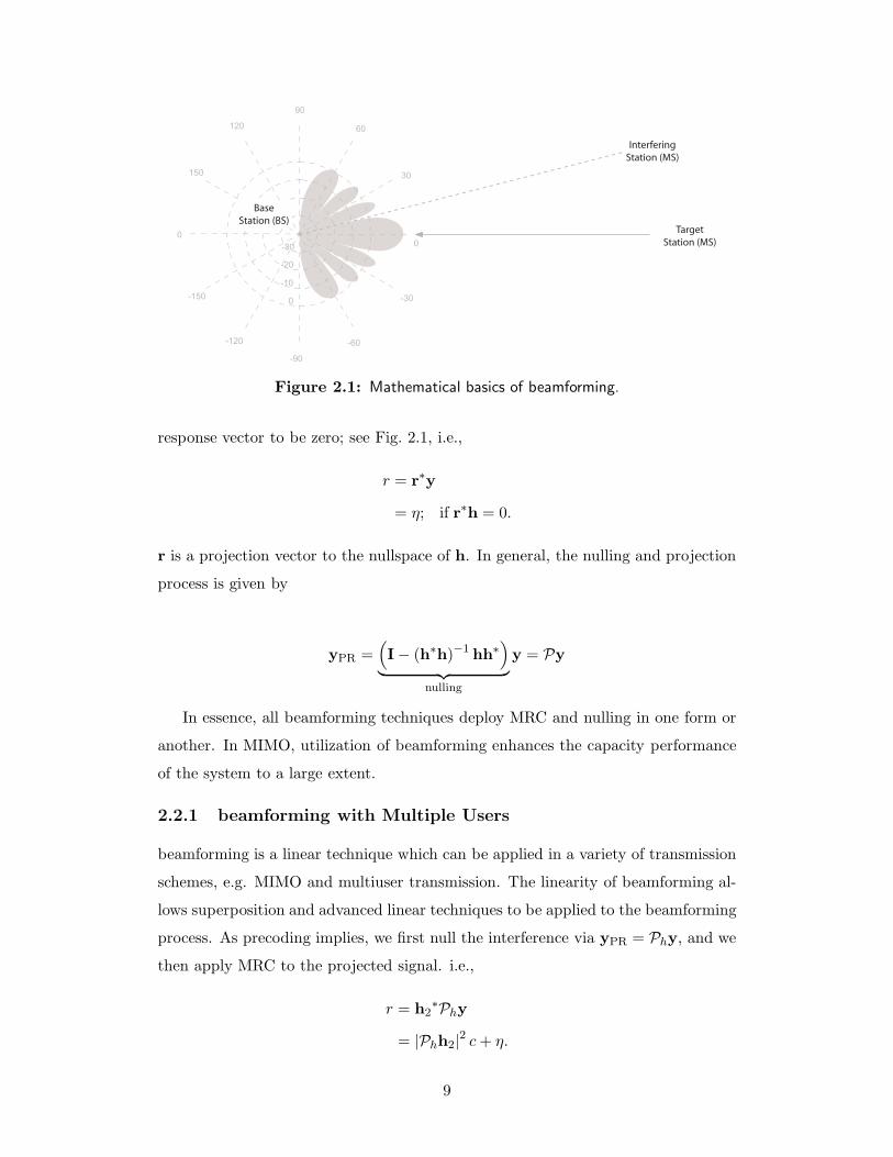
output of antenna arrays by means of spatial filtering. Fig. 2.1 shows the basics of

beamforming to a target MS. The complex vector y = hc, where

h = [h1, . . . , hN ]

is received by all N received antennas.

To detect the signal, the receiver then applies maximum ratio combining (MRC)

on the received vector y,

r = h∗y

=

M∑

m=1

|hm|2c+ η (2.1)

The detection process of signal-of-interest can be yet extended to nulling the un-

wanted signals. By forcing the inner product of the received signal and the processed

8

150

-150

-30

-20

-10

0

30

60

-120

90

-90

120

-60

-30

0

0

Base

Station (BS)

Interfering

Station (MS)

Target

Station (MS)

Figure 2.1: Mathematical basics of beamforming.

response vector to be zero; see Fig. 2.1, i.e.,

r = r∗y

= η; if r∗h = 0.

r is a projection vector to the nullspace of h. In general, the nulling and projection

process is given by

yPR =(

I− (h∗h)−1 hh∗)

︸ ︷︷ ︸

nulling

y = Py

In essence, all beamforming techniques deploy MRC and nulling in one form or

another. In MIMO, utilization of beamforming enhances the capacity performance

of the system to a large extent.

2.2.1 beamforming with Multiple Users

beamforming is a linear technique which can be applied in a variety of transmission

schemes, e.g. MIMO and multiuser transmission. The linearity of beamforming al-

lows superposition and advanced linear techniques to be applied to the beamforming

process. As precoding implies, we first null the interference via yPR = Phy, and we

then apply MRC to the projected signal. i.e.,

r = h2∗Phy

= |Phh2|2 c+ η.

9

150

-150

-30

-20

-10

0

30

60

-120

90

-90

120

-60

-30

0

0

Base

Station (BS)Target 2

Station (MS)

Target 1

Station (MS)

Target 2

Station (MS)

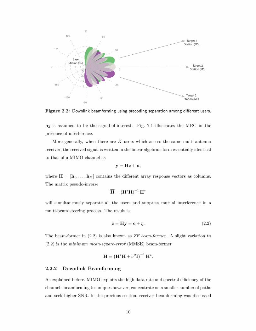
Figure 2.2: Downlink beamforming using precoding separation among different users.

h2 is assumed to be the signal-of-interest. Fig. 2.1 illustrates the MRC in the

presence of interference.

More generally, when there are K users which access the same multi-antenna

receiver, the received signal is written in the linear algebraic form essentially identical

to that of a MIMO channel as

y = Hc+ n,

where H = [h1, . . . ,hK ] contains the different array response vectors as columns.

The matrix pseudo-inverse

H = (H∗H)−1 H∗

will simultaneously separate all the users and suppress mutual interference in a

multi-beam steering process. The result is

c = Hy = c+ η. (2.2)

The beam-former in (2.2) is also known as ZF beam-former. A slight variation to

(2.2) is the minimum mean-square-error (MMSE) beam-former

H =(H∗H+ σ2I

)−1H∗.

2.2.2 Downlink Beamforming

As explained before, MIMO exploits the high data rate and spectral efficiency of the

channel. beamforming techniques however, concentrate on a smaller number of paths

and seek higher SNR. In the previous section, receiver beamforming was discussed

10

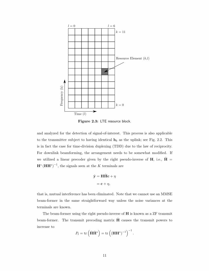
Figure 2.3: LTE resource block.

and analyzed for the detection of signal-of-interest. This process is also applicable

to the transmitter subject to having identical hk as the uplink; see Fig. 2.2. This

is in fact the case for time-division duplexing (TDD) due to the law of reciprocity.

For downlink beamforming, the arrangement needs to be somewhat modified. If

we utilized a linear precoder given by the right pseudo-inverse of H, i.e., H =

H∗ (HH∗)−1, the signals seen at the K terminals are

y = HHc+ η

= c+ η,

that is, mutual interference has been eliminated. Note that we cannot use an MMSE

beam-former in the same straightforward way unless the noise variances at the

terminals are known.

The beam-former using the right pseudo-inverse of H is known as a ZF transmit

beam-former. The transmit precoding matrix H causes the transmit powers to

increase to

Pt = tr(

HH∗)

= tr(

(HH∗)−1)−1

.

11

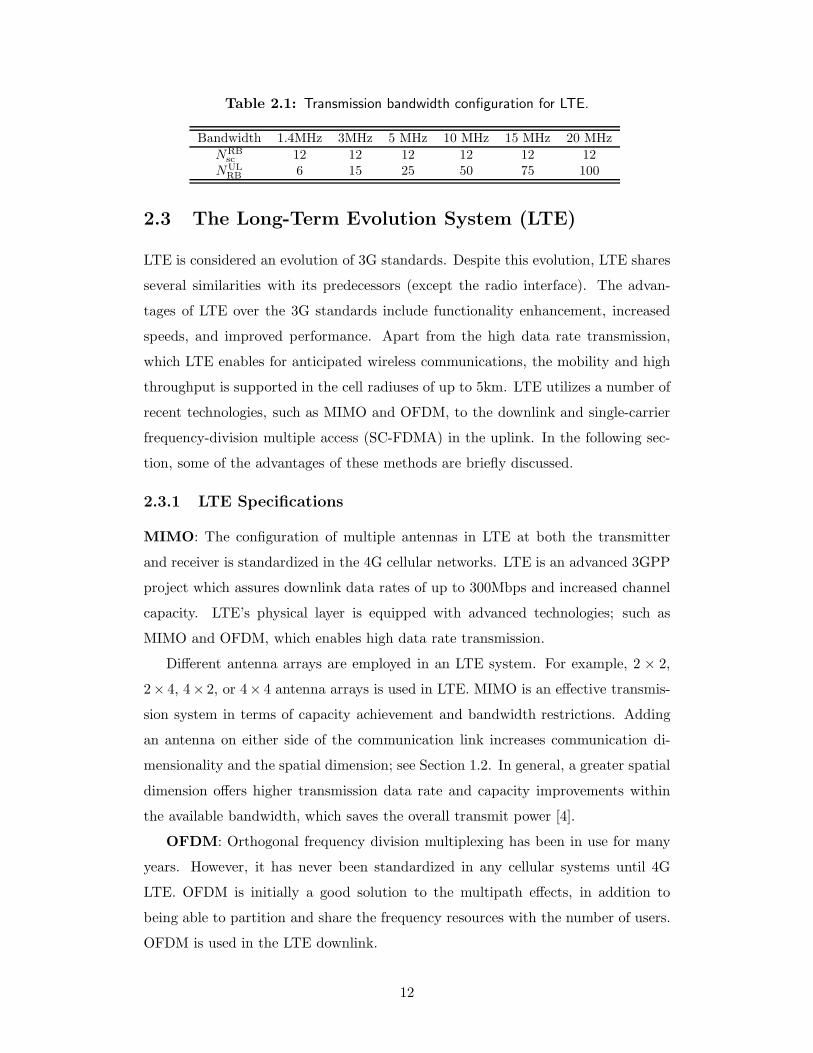
Table 2.1: Transmission bandwidth configuration for LTE.

Bandwidth 1.4MHz 3MHz 5 MHz 10 MHz 15 MHz 20 MHz

NRBsc 12 12 12 12 12 12

NUL

RB6 15 25 50 75 100

2.3 The Long-Term Evolution System (LTE)

LTE is considered an evolution of 3G standards. Despite this evolution, LTE shares

several similarities with its predecessors (except the radio interface). The advan-

tages of LTE over the 3G standards include functionality enhancement, increased

speeds, and improved performance. Apart from the high data rate transmission,

which LTE enables for anticipated wireless communications, the mobility and high

throughput is supported in the cell radiuses of up to 5km. LTE utilizes a number of

recent technologies, such as MIMO and OFDM, to the downlink and single-carrier

frequency-division multiple access (SC-FDMA) in the uplink. In the following sec-

tion, some of the advantages of these methods are briefly discussed.

2.3.1 LTE Specifications

MIMO: The configuration of multiple antennas in LTE at both the transmitter

and receiver is standardized in the 4G cellular networks. LTE is an advanced 3GPP

project which assures downlink data rates of up to 300Mbps and increased channel

capacity. LTE’s physical layer is equipped with advanced technologies; such as

MIMO and OFDM, which enables high data rate transmission.

Different antenna arrays are employed in an LTE system. For example, 2 × 2,

2× 4, 4× 2, or 4× 4 antenna arrays is used in LTE. MIMO is an effective transmis-

sion system in terms of capacity achievement and bandwidth restrictions. Adding

an antenna on either side of the communication link increases communication di-

mensionality and the spatial dimension; see Section 1.2. In general, a greater spatial

dimension offers higher transmission data rate and capacity improvements within

the available bandwidth, which saves the overall transmit power [4].

OFDM: Orthogonal frequency division multiplexing has been in use for many

years. However, it has never been standardized in any cellular systems until 4G

LTE. OFDM is initially a good solution to the multipath effects, in addition to

being able to partition and share the frequency resources with the number of users.

OFDM is used in the LTE downlink.

12

Frame Block

Subframe

Slot

CP Symbol

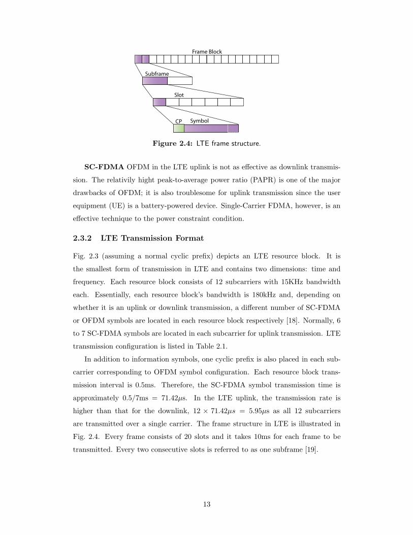
Figure 2.4: LTE frame structure.

SC-FDMA OFDM in the LTE uplink is not as effective as downlink transmis-

sion. The relativily hight peak-to-average power ratio (PAPR) is one of the major

drawbacks of OFDM; it is also troublesome for uplink transmission since the user

equipment (UE) is a battery-powered device. Single-Carrier FDMA, however, is an

effective technique to the power constraint condition.

2.3.2 LTE Transmission Format

Fig. 2.3 (assuming a normal cyclic prefix) depicts an LTE resource block. It is

the smallest form of transmission in LTE and contains two dimensions: time and

frequency. Each resource block consists of 12 subcarriers with 15KHz bandwidth

each. Essentially, each resource block’s bandwidth is 180kHz and, depending on

whether it is an uplink or downlink transmission, a different number of SC-FDMA

or OFDM symbols are located in each resource block respectively [18]. Normally, 6

to 7 SC-FDMA symbols are located in each subcarrier for uplink transmission. LTE

transmission configuration is listed in Table 2.1.

In addition to information symbols, one cyclic prefix is also placed in each sub-

carrier corresponding to OFDM symbol configuration. Each resource block trans-

mission interval is 0.5ms. Therefore, the SC-FDMA symbol transmission time is

approximately 0.5/7ms = 71.42µs. In the LTE uplink, the transmission rate is

higher than that for the downlink, 12 × 71.42µs = 5.95µs as all 12 subcarriers

are transmitted over a single carrier. The frame structure in LTE is illustrated in

Fig. 2.4. Every frame consists of 20 slots and it takes 10ms for each frame to be

transmitted. Every two consecutive slots is referred to as one subframe [19].

13

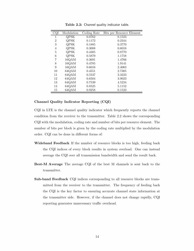
Table 2.2: Channel quality indicator table.

CQI Modulation Coding Rate Bits per Resource Element

1 QPSK 0.0762 0.15232 QPSK 0.1172 0.23443 QPSK 0.1885 0.37704 QPSK 0.3008 0.60165 QPSK 0.4385 0.87706 QPSK 0.5879 1.17587 16QAM 0.3691 1.47668 16QAM 0.4785 1.91419 16QAM 0.6016 2.406310 64QAM 0.4551 2.730511 64QAM 0.5537 3.322312 64QAM 0.6504 3.902313 64QAM 0.7539 4.523414 64QAM 0.8525 5.115215 64QAM 0.9258 0.1523

Channel Quality Indicator Reporting (CQI)

CQI in LTE is the channel quality indicator which frequently reports the channel

condition from the receiver to the transmitter. Table 2.2 shows the corresponding

CQI with the modulation, coding rate and number of bits per resource element. The

number of bits per block is given by the coding rate multiplied by the modulation

order. CQI can be done in different forms of:

Wideband Feedback If the number of resource blocks is too high, feeding back

the CQI indices of every block results in system overload. One can instead

average the CQI over all transmission bandwidth and send the result back.

Best-M Average The average CQI of the best M channels is sent back to the

transmitter.

Sub-band Feedback CQI indices corresponding to all resource blocks are trans-

mitted from the receiver to the transmitter. The frequency of feeding back

the CQI is the key factor to ensuring accurate channel state information at

the transmitter side. However, if the channel does not change rapidly, CQI

reporting generates unnecessary traffic overhead.

14

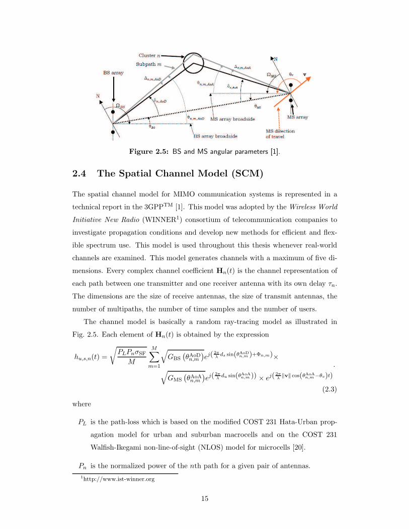
Figure 2.5: BS and MS angular parameters [1].

2.4 The Spatial Channel Model (SCM)

The spatial channel model for MIMO communication systems is represented in a

technical report in the 3GPPTM [1]. This model was adopted by the Wireless World

Initiative New Radio (WINNER1) consortium of telecommunication companies to

investigate propagation conditions and develop new methods for efficient and flex-

ible spectrum use. This model is used throughout this thesis whenever real-world

channels are examined. This model generates channels with a maximum of five di-

mensions. Every complex channel coefficient Hn(t) is the channel representation of

each path between one transmitter and one receiver antenna with its own delay τn.

The dimensions are the size of receive antennas, the size of transmit antennas, the

number of multipaths, the number of time samples and the number of users.

The channel model is basically a random ray-tracing model as illustrated in

Fig. 2.5. Each element of Hn(t) is obtained by the expression

hu,s,n(t) =

√

PLPnσSFM

M∑

m=1

√

GBS

(θAoDn,m

)ej(

2πλds sin(θAoD

n,m )+Φn,m)×√

GMS

(θAoAn,m

)ej(

2πλdu sin(θAoA

n,m )) × ej(2πλ‖v‖ cos(θAoA

n,m−θv)t)

.

(2.3)

where

PL is the path-loss which is based on the modified COST 231 Hata-Urban prop-

agation model for urban and suburban macrocells and on the COST 231

Walfish-Ikegami non-line-of-sight (NLOS) model for microcells [20].

Pn is the normalized power of the nth path for a given pair of antennas.

1http://www.ist-winner.org

15

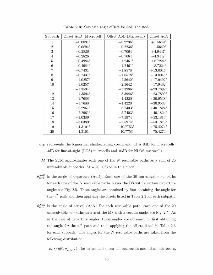
Table 2.3: Sub-path angle offsets for AoD and AoA.

Subpath Offset AoD (Macrocell) Offset AoD (Microcell) Offset AoA

1 +0.0894◦ +0.2236◦ +1.5649◦

2 −0.0894◦ −0.2236◦ −1.5649◦

3 +0.2826◦ +0.7064◦ +4.9447◦

4 −0.2826◦ −0.7064◦ −4.9447◦

5 +0.4984◦ +1.2461◦ +8.7224◦

6 −0.4984◦ −1.2461◦ −8.7224◦

7 +0.7431◦ +1.8578◦ +13.0045◦

8 −0.7431◦ −1.8578◦ −13.0045◦

9 +1.0257◦ +2.5642◦ +17.9492◦

10 −1.0257◦ −2.5642◦ −17.9492◦

11 +1.3594◦ +3.3986◦ +23.7899◦

12 −1.3594◦ −3.3986◦ −23.7899◦

13 +1.7688◦ +4.4220◦ +30.9538◦

14 −1.7688◦ −4.4220◦ −30.9538◦

15 +2.2961◦ +5.7403◦ +40.1824◦

16 −2.2961◦ −5.7403◦ −40.1824◦

17 +3.0389◦ +7.5974◦ +53.1816◦

18 −3.0389◦ −7.5974◦ −53.1816◦

19 +4.3101◦ +10.7753◦ +75.4274◦

20 −4.3101◦ −10.7753◦ −75.4274◦

σSF represents the lognormal shadowfading coefficient. It is 8dB for macrocells,

4dB for line-of-sight (LOS) microcells and 10dB for NLOS microcells.

M The SCM approximates each one of the N resolvable paths as a sum of 20

unresolvable subpaths. M = 20 is fixed in this model.

θAoDn,m is the angle of departure (AoD). Each one of the 20 unresolvable subpaths

for each one of the N resolvable paths leaves the BS with a certain departure

angle; see Fig. 2.5. These angles are obtained by first obtaining the angle for

the nth path and then applying the offsets listed in Table 2.3 for each subpath.

θAoAn,m is the angle of arrival (AoA) For each resolvable path, each one of the 20

unresolvable subpaths arrives at the MS with a certain angle; see Fig. 2.5. As

in the case of departure angles, these angles are obtained by first obtaining

the angle for the nth path and then applying the offsets listed in Table 2.3

for each subpath. The angles for the N resolvable paths are taken from the

following distribution

ρn ∼ η(0, σ2n,AoA) for urban and suburban macrocells and urban microcells,

16

where

σn,AoA = 104.12(

1− e−0.2175|10 log(Pn)|)

and

σn,AoA = 104.12(

1− e−0.265|10 log(Pn)|)

for macrocells and microcells, respectively. These angles are associated with

randomly chosen resolvable paths.

GBS

(θAoDn,m

)is BS antenna gain. Since the BS antennas are sectorized, its gain depends on

the departure angle, as seen in Section 4.5.1 of [1].

(GMSθ

AoAn,m

)is mobile antenna gain at MS which is assumed to have an omni-directional

pattern with a gain of −1dB.

λ represents the carrier wavelength in meters.

ds is the distance of the sth antenna from the reference antenna at the BS; given

in meters.

du is the distance of the uth antenna from the reference antenna at the MS; given

in meters.

Φn,m is the phase of the mth subpath of the mth path. Subpaths are (i.i.d.) with a

uniform distribution in the interval [0, 2π].

‖v‖ is the magnitude of the MS velocity vector.

θv represents the angle of the MS velocity vector with respect to the MS broad-

side; see Fig. 2.5.

The random delays for each one of the n multipaths are obtained by first gener-

ating the following random variables:

τ ′n =

{

−rDSσDS ln(zn), for urban and suburban macrocells;

z′n, for urban microcells;

where zn is a random variable with uniform distribution U(0, 1), rDS = 1.4µs for

suburban macrocells, rDS = 1.7µs for urban macrocells and σDS is derived at the

end of this section. The variable z′n is a uniform random variable in the interval 0

to 1.2µs. These variables are sorted in descending order, i.e., τ ′N > τ ′N−1 > · · · > τ ′1.

17

According to this definition, τ ′1 = 0. The delay from the nth path, denoted by τn, is

then quantized according to (2.4):

τn =TC16

⌊

τ ′n − τ ′1TC

16

+1

2

⌋

, (2.4)

where TC is the duration of a chip interval.

18

Chapter 3

Channel Estimation

3.1 The Estimation Problem

In a real-world environment, the transmission channel used by a communication

system is not stationary and undergoes changes with time, sometimes rapidly. Such

a channel can be modeled by (2.3). To establish reliable communication, the MIMO

methods explained in the previous chapter can be utilized for the communication

systems if the channel is known; see Section 2. However, three difficulties arise when

the channel is required by the communications system:

1. Channel knowledge must be acquired by the receiver (channel estimation)

2. The channel knowledge must be fed back to the transmitter (see Chapter 4)

3. If the channel changes significantly, the channel knowledge at the transmitter

becomes inaccurate and outdated, this is known as data aging. (We do not

consider this issue here.)

Channel estimation is a fundamental operation required by every communica-

tion system. For this reason,this entire chapter is devoted to the basis of estimation

algorithms. Estimation is typically done in three ways: filtering, smoothing and

prediction. Filtering and prediction are real-time operations. Filtering at time t is

done using data received prior to time t. Prediction is estimation of the process at

time t + τ using data measured at time t and earlier. Second-order statistics (i.e.,

mean and correlation functions) of signals and noise are required in this computa-

tion. The main approach to the filtering problem, i.e., channel estimation, is the

minimization of mean-square errors. This error is defined as the power difference

between the desired response and the filter output.

19

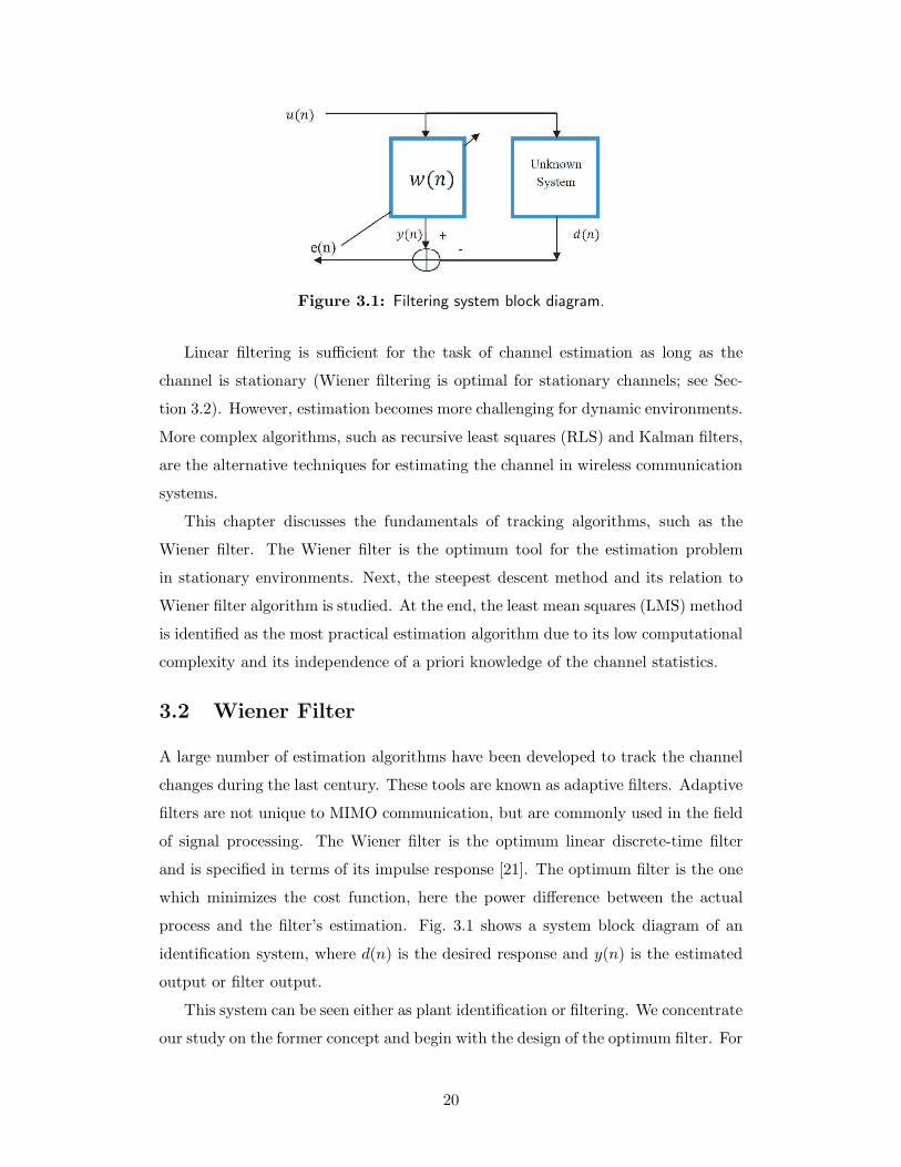
Figure 3.1: Filtering system block diagram.

Linear filtering is sufficient for the task of channel estimation as long as the

channel is stationary (Wiener filtering is optimal for stationary channels; see Sec-

tion 3.2). However, estimation becomes more challenging for dynamic environments.

More complex algorithms, such as recursive least squares (RLS) and Kalman filters,

are the alternative techniques for estimating the channel in wireless communication

systems.

This chapter discusses the fundamentals of tracking algorithms, such as the

Wiener filter. The Wiener filter is the optimum tool for the estimation problem

in stationary environments. Next, the steepest descent method and its relation to

Wiener filter algorithm is studied. At the end, the least mean squares (LMS) method

is identified as the most practical estimation algorithm due to its low computational

complexity and its independence of a priori knowledge of the channel statistics.

3.2 Wiener Filter

A large number of estimation algorithms have been developed to track the channel

changes during the last century. These tools are known as adaptive filters. Adaptive

filters are not unique to MIMO communication, but are commonly used in the field

of signal processing. The Wiener filter is the optimum linear discrete-time filter

and is specified in terms of its impulse response [21]. The optimum filter is the one

which minimizes the cost function, here the power difference between the actual

process and the filter’s estimation. Fig. 3.1 shows a system block diagram of an

identification system, where d(n) is the desired response and y(n) is the estimated

output or filter output.

This system can be seen either as plant identification or filtering. We concentrate

our study on the former concept and begin with the design of the optimum filter. For

20

optimization of the identification filter, the cost function should be minimized. The

cost function is the mean-square value of the estimation error which is defined as the

difference between the desired output and the filter output. Minimum mean square

estimation (MMSE) leads to a set of equations known as the Wiener-hopf equations

to be discussed shortly. In practice, solution of these equations requires second-order

statistical knowledge of the channel, which increases the computational complexity.

Different mathematical approaches have been employed to solve for Wiener-hopf

equation and simplify the procedures. Two approaches are considered which lead to

tractable mathematics. One is the principle of orthogonality, and the other is the

error performance surface.

3.2.1 Principle of Orthogonality

Considering the block diagram shown in Fig. 3.1, the output of the unknown system

is estimated by

y(n) =

L−1∑

k=0

w∗ku(n − k) (3.1)

which illustrates an inner product of the filter coefficients wk and the system input

u(n− k). The filter input and the desired response are assumed to be jointly wide-

sense stationary stochastic processes with zero mean. Then, the estimation error is

the random sample of time n given by

e(n) = d(n)− y(n) (3.2)

and the cost function is defined in (3.3), realizing that the input data and the filter

coefficients are complex values:

J = E[e(n)e∗(n)] = E[|e(n)|2] (3.3)

Solving for optimization, the cost function needs to be minimized. In that case,

a gradient operator is used to migrate towards the stationary point of the cost

function:

∇k(J) = −2 E[u(n− k)e∗(n)]; k = 1, 2, ..., L. (3.4)

Equating (3.4) to zero gives necessary and sufficient condition for J to attain its

minimum value. Note that the kth derivative is taken with respect to wk. Therefore,

the corresponding value of e(n) must be orthogonal to each input sample, where

21

orthogonality between two sequences of u and v is defined as E[u(n)v∗(n)]. Using

this orthogonality principle, the correlation between the filter outputs y(n) and error

estimation can be expressed as

E[y(n)e∗(n)] =L−1∑

k=0

w∗kE[u(n− k)e∗(n)]

This implies that the estimated outputs y(n) and the corresponding estimation error

e(n) are orthogonal as well. In this approach, we substitute equations (3.1) and (3.2)

into

E[u(n− k)e∗(n)] = 0, k = 0, 1, 2, . . . , L− 1

to obtain

E[u(n− k)(d∗(n)−L−1∑

i=0

woiu∗(n− i))] = 0, k = 0, 1, 2, . . . , L− 1

or

L−1∑

i=0

woiE[u(n− k)u∗(n− i)] = E[u(n − k)d∗(n)]. k = 0, 1, 2, . . . , L− 1 (3.5)

Defining terms as:

r(i− k) = E[u(n− k)u∗(n− i)] (3.6)

p(−k) = E[u(n− k)d∗(n)] (3.7)

where (3.6) is the auto-correlation of the filter inputs and (3.7) is the cross-correlation

between the filter input and the desired response (output of the unknown system).

Therefore, equation (3.5) can be rewritten as

L∑

i=0

woir(i− k) = p(−k), k = 0, 1, 2, . . . , L− 1

These are the so-called Wiener-Hopf equations, which can be solved efficiently based

on spectral factorization. Another approach can be taken to tackle this problem.

Using (3.2) and (3.3),

e(n) = d(n)−L−1∑

k=0

w∗ku(n− k),

and

22

J = E[|d(n)|2]−L−1∑

k=0

w∗kE[u(n− k)d∗(n)]

−L−1∑

k=0

wkE[u(n− k)d(n)] +

L−1∑

k=0

L−1∑

i=0

w∗kwiE[u(n− k)u∗(n− i)]

The above equation can be simplified to

J = σ2d −L−1∑

i=0

w∗kp(−k)−

L−1∑

i=0

wkp∗(−k) +

L−1∑

i=0

w∗kwir(n− i)

which implies that the cost function is a second-order function of the filter tap-

weights. The dependence of the cost function on the tap weights can be visualized

as a bowl-shaped, L + 1-dimensional surface with L degrees of freedom. At the

bottom of the error-surface, the cost function attains its minimum value. This can

be represented as follows:

∇k(J) =∂J

∂ak+ j

∂J

∂bk(3.8)

where ak and bk are real and imaginary components of wk. Then,

∇k(J) = −2p(−k) + 2

L−1∑

i=0

wir(i− k)

The optimal point is reached when ∇k = 0, or equivalently,

p(−k) =L−1∑

i=0

woir(i− k), k = 0, 1, 2, . . .

which is equivalent to Wiener-Hopf equation.

We have shown that, in order to come up with an optimum system, different

approaches may be taken. Applying the gradient operation over the cost function

results in an optimum filter, and its performance will be studied over the error

performance surface. In this approach, it has also been proved that the estimation

error is orthogonal to the actual output of the filter.

3.3 Methods of Steepest Descent (SD) and LMS Algo-

rithm

To set up the problem in the context of this thesis, a filter which is less complex

and more robust to fast changes - in our case, the channel - is our primary interest.

23

The goal is to track the channel in order to generate a sufficiently good estimate

of the channel statistics, which can then be used to predict the channel’s future

behavior. The SD technique belongs to the family of iterative methods of opti-

mization and it provides a method of searching for a multidimensional performance

surface. This is a gradient-based method which means that the algorithm follows

the local gradient. The steepest descent method is therefore a recursive algorithm

which starts from some initial value of the solution, and it tends to improve with

the number of iterations. SD is akin to a multiparameter closed-loop determinis-

tic control system which finds the minimum-point of the error-performance surface

without knowledge of surface itself, giving basic clues that lead to the development

of the LMS algorithm.

3.3.1 The SD Algorithm

The input sequence to our system, u(n), u(n−1), . . . , u(n−M+1) is assumed to be a

wide-sense stationary stochastic process of zero-mean and correlation matrixR. The

corresponding desired response at the filter output is denoted by y(n) = wH(n)u(n)

and the filter tap-weights are wn, w1, ..., wn−M+1. Note that the input vector u(n)

and d(n) are assumed to be jointly stationary.

Applying 3.2 the cost function is:

J(n) = σ2d −wH(n)p− pHw(n) +wH(n)Rw(n)

which is equivalent to the estimation of the mean square error to be minimized.

As has been already mentioned, the cost function is quadratic in the tap-weight

vector. The error performance surface is a visualization of the dependence of the

mean-squared error on the elements of the vector w(n) as a bowl shape. An adaptive

process continually seeks the bottom or minimum point of this surface. Let w0 be

the optimal solution defined by Wiener-hopf equations:

Rw0 = p

Therefore, the minimum value of the cost function can be followed:

Jmin = σ2d − pHR−1p

where

σ2y = E[wH0 u(n)uH(n)w0] = wH

0 E[u(n)uH ]w0

24

and

Jmin = σ2d − σ2y

.

The algorithm for SD is obtained as follows:

1. Start the algorithm with an initial w0 which can be set to zero.

2. Evaluate the gradient from (3.8).

3. Compute the next tap-weight vector by making a change in the initial or

present vector in a direction opposite to that of the gradient vector. This is

done as

w(n + 1) = w(n) +1

2[−∇(J(n))], (3.9)

One half is the step size parameter which helps the algorithm to converge

faster.

4) Go back to step 2.

The gradient in (3.9) is given by

∇(J(n)) = −2p+ 2Rw(n),

and

w(n+ 1) = w(n) + [p−Rw(n)],

which p−Rw(n) is the correction weight vector.

Note that, from (3.4),

E[u(n)eH(n)] = −∇(J(n)) = −∇(E[e(n)eH(n)]). (3.10)

This shows that at Jmin, input sequence u(n) is orthogonal to the error sequence.

3.3.2 Stochastic Gradient-Based Algorithms: the LMS Approach

One of the most important features of stochastic gradient-based algorithms (SGBA)

e.g. the LMS algorithm, is their simplicity. In the LMS algorithm, measurement

of the correlation function and the performance of matrix inversion is not required.

The value of the tap-weight vector w(n) using LMS represents an estimate of w(n)

whose expected value approaches the Wiener filter (w0), for a wide-sense stationary

(WSS) process as n approaches infinity.

25

In the LMS algorithm an approximation to (3.10) is used to compute w(n + 1)

from w(n)

u(n)e∗(n) = w(n + 1)− w(n) = δw(n).

Basically, the LMS algorithm avoids the operation of expectation. For this reason,

it is a less complex and is the most widely used algorithm. In the LMS algorithm,

the tap-weight vector w(n) is not exactly the one which will be evaluated from

the SD algorithm. w(n) executes a random motion around the minimum point of

the error performance surface, which requires the step-size-parameter µ to satisfy

conditions related to the eigenvalues of the random correlation matrix R of the

tap-inputs. In the LMS algorithm, an adaptive mechanism is utilized in place of a

deterministic approach in SD. This way, there is a penalty for misadjustment given

by ratio JLMS(∞)/JSD This leads to the following:

1. The LMS converges to the mean E[w(n)] = w0, which is the Wiener solution

as n→ ∞

2. The LMS converges to the mean square JLMS(n) → JSD(∞) as n→ ∞

As was shown earlier, the exact solution of ∇(J(n)) leads to the Wiener solution

w0, however it needs a priori knowledge of R (the autocorrelation of the tap inputs)

and p (the cross correlation of u and d). The LMS algorithm estimates the gradient

from instantaneous data. In other words, the tap-weight vector is updated in accor-

dance with an algorithm that adapts to the incoming data instead of measurement

of R and p, which are estimated as

R(n) = u(n)uH(n),

and

p(n) = u(n)d∗(n),

Therefore,

∇JLMS(n) = −2u(n)d∗(n) + 2u(n)uH(n)w(n).

This shows that the estimation is biased since the tap-weight vector w(n) is a

random vector that depends on the vector u(n). The recursive relation for computing

the tap-weight vector is finally given by

w(n+ 1) = w(n) + µu(n)[d∗(n)− uH(n)w(n)]

and µ is constrained by 0 < µ < 2/total input power.

26

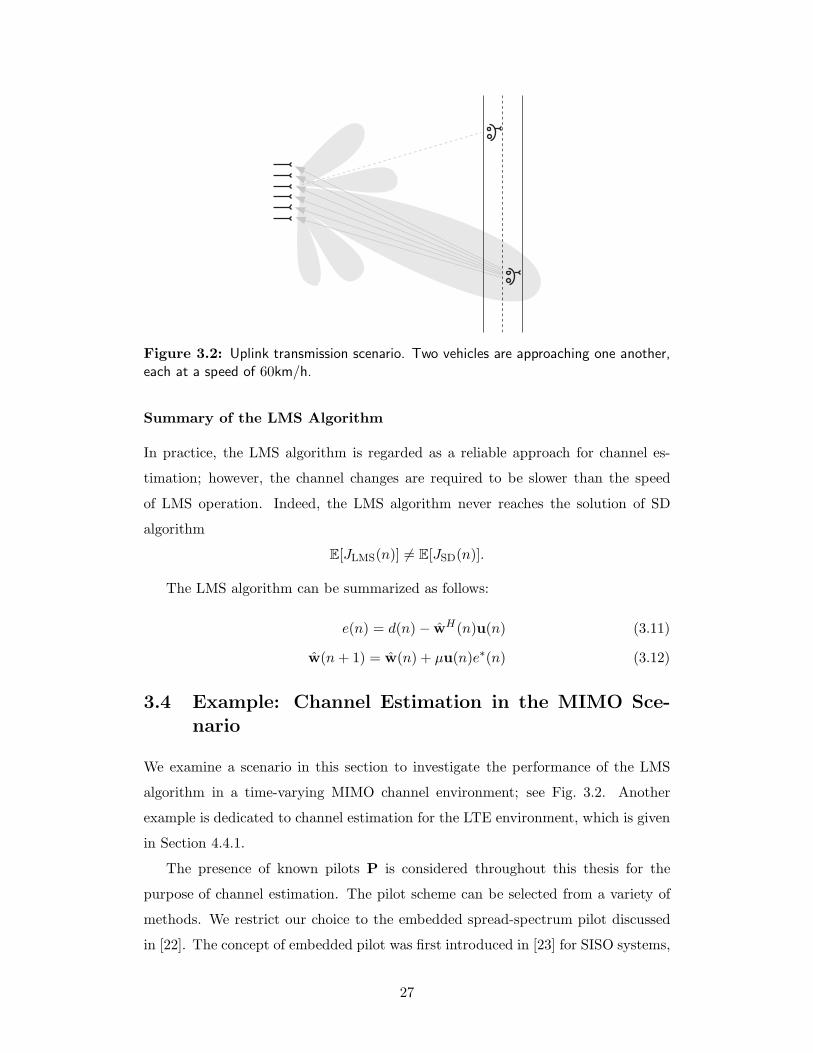
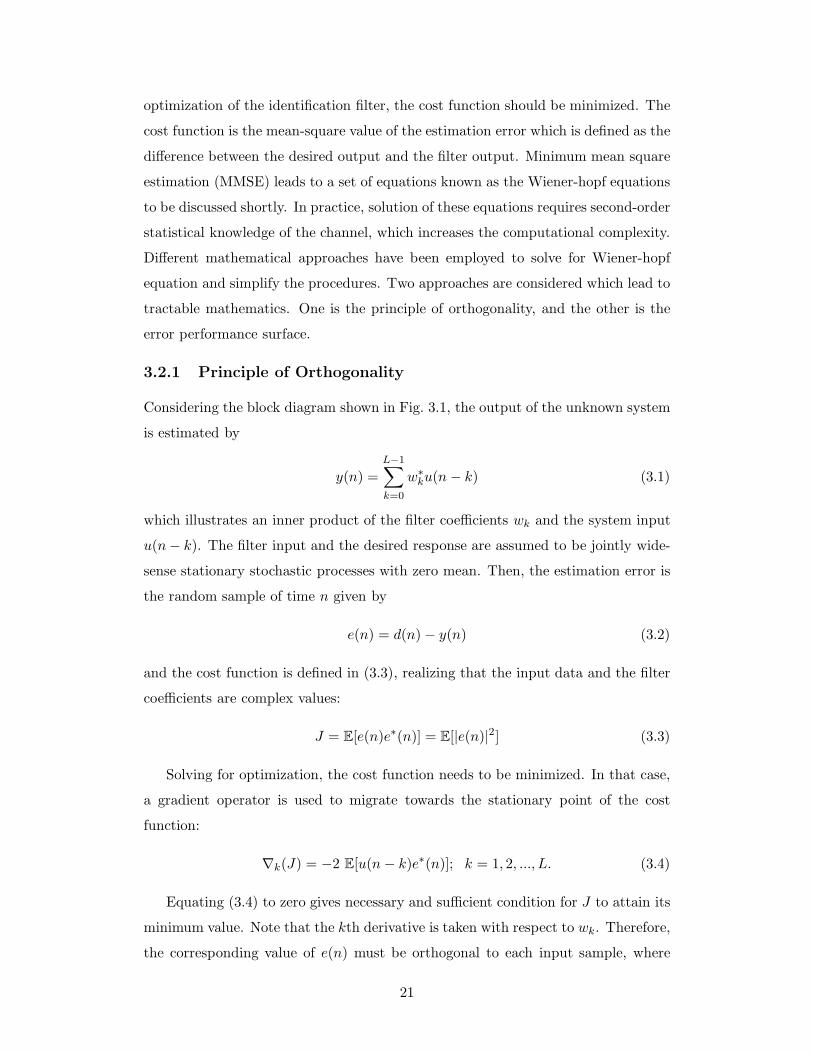
Figure 3.2: Uplink transmission scenario. Two vehicles are approaching one another,each at a speed of 60km/h.

Summary of the LMS Algorithm

In practice, the LMS algorithm is regarded as a reliable approach for channel es-

timation; however, the channel changes are required to be slower than the speed

of LMS operation. Indeed, the LMS algorithm never reaches the solution of SD

algorithm

E[JLMS(n)] 6= E[JSD(n)].

The LMS algorithm can be summarized as follows:

e(n) = d(n)− wH(n)u(n) (3.11)

w(n+ 1) = w(n) + µu(n)e∗(n) (3.12)

3.4 Example: Channel Estimation in the MIMO Sce-nario

We examine a scenario in this section to investigate the performance of the LMS

algorithm in a time-varying MIMO channel environment; see Fig. 3.2. Another

example is dedicated to channel estimation for the LTE environment, which is given

in Section 4.4.1.

The presence of known pilots P is considered throughout this thesis for the

purpose of channel estimation. The pilot scheme can be selected from a variety of

methods. We restrict our choice to the embedded spread-spectrum pilot discussed

in [22]. The concept of embedded pilot was first introduced in [23] for SISO systems,

27

0 2 4 6 8 10−6

−4

−2

0

2

4

6

Time [sec]

Amplitude

Channel

LMS Estimation

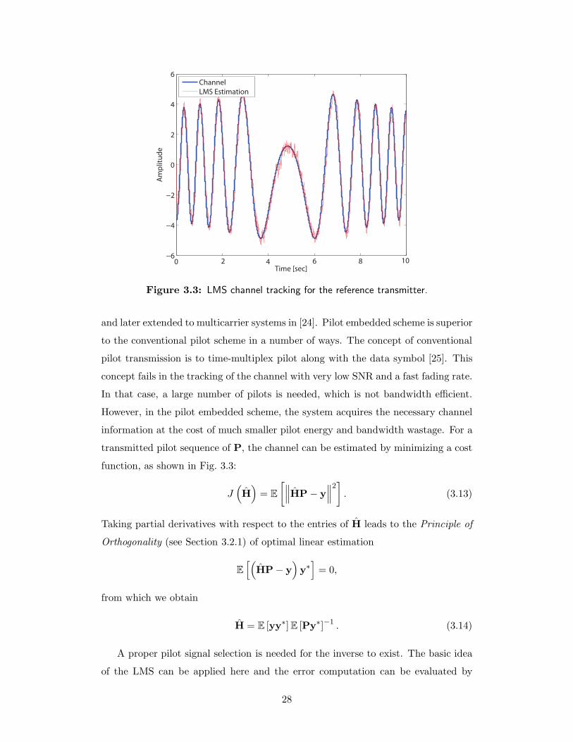
Figure 3.3: LMS channel tracking for the reference transmitter.

and later extended to multicarrier systems in [24]. Pilot embedded scheme is superior

to the conventional pilot scheme in a number of ways. The concept of conventional

pilot transmission is to time-multiplex pilot along with the data symbol [25]. This

concept fails in the tracking of the channel with very low SNR and a fast fading rate.

In that case, a large number of pilots is needed, which is not bandwidth efficient.

However, in the pilot embedded scheme, the system acquires the necessary channel

information at the cost of much smaller pilot energy and bandwidth wastage. For a

transmitted pilot sequence of P, the channel can be estimated by minimizing a cost

function, as shown in Fig. 3.3:

J(

H)

= E

[∥∥∥HP− y

∥∥∥

2]

. (3.13)

Taking partial derivatives with respect to the entries of H leads to the Principle of

Orthogonality (see Section 3.2.1) of optimal linear estimation

E

[(

HP− y)

y∗]

= 0,

from which we obtain

H = E [yy∗]E [Py∗]−1 . (3.14)

A proper pilot signal selection is needed for the inverse to exist. The basic idea

of the LMS can be applied here and the error computation can be evaluated by

28

0 5 10 15 20−0.2

0

0.2

0.4

0.6

0.8

Lag

Sample autocorrelation

Co

n�

de

nce

inte

rva

l

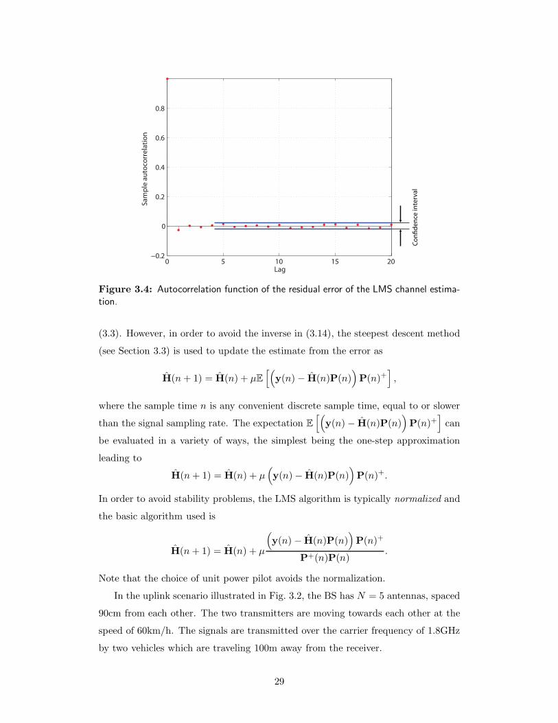
Figure 3.4: Autocorrelation function of the residual error of the LMS channel estima-tion.

(3.3). However, in order to avoid the inverse in (3.14), the steepest descent method

(see Section 3.3) is used to update the estimate from the error as

H(n+ 1) = H(n) + µE[(

y(n)− H(n)P(n))

P(n)+]

,

where the sample time n is any convenient discrete sample time, equal to or slower

than the signal sampling rate. The expectation E

[(

y(n)− H(n)P(n))

P(n)+]

can

be evaluated in a variety of ways, the simplest being the one-step approximation

leading to

H(n+ 1) = H(n) + µ(

y(n)− H(n)P(n))

P(n)+.

In order to avoid stability problems, the LMS algorithm is typically normalized and

the basic algorithm used is

H(n+ 1) = H(n) + µ

(

y(n) − H(n)P(n))

P(n)+

P+(n)P(n).

Note that the choice of unit power pilot avoids the normalization.

In the uplink scenario illustrated in Fig. 3.2, the BS has N = 5 antennas, spaced

90cm from each other. The two transmitters are moving towards each other at the

speed of 60km/h. The signals are transmitted over the carrier frequency of 1.8GHz

by two vehicles which are traveling 100m away from the receiver.

29

−5 0 5

−10

−5

0

5

Time relative to passing [sec]

Pro

ject

ion

loss

aft

er

sup

pre

ssin

g in

terf

ere

r [d

B]

Figure 3.5: Projection loss for two passing transmitters.

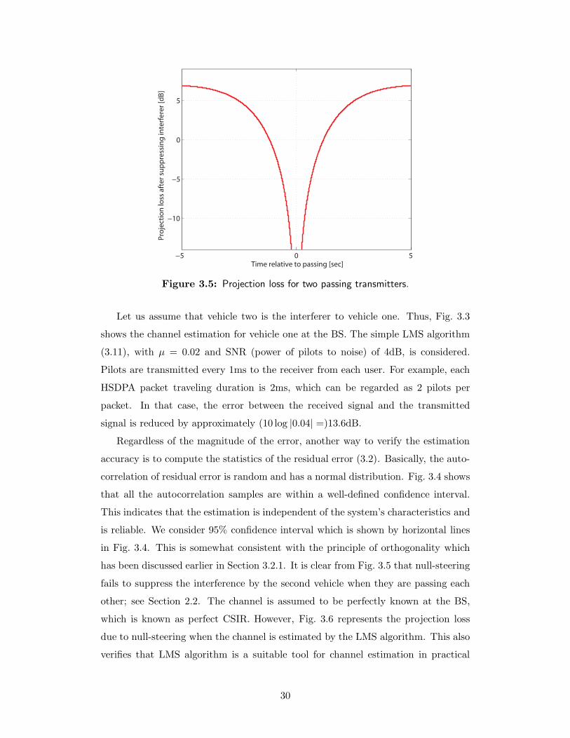
Let us assume that vehicle two is the interferer to vehicle one. Thus, Fig. 3.3

shows the channel estimation for vehicle one at the BS. The simple LMS algorithm

(3.11), with µ = 0.02 and SNR (power of pilots to noise) of 4dB, is considered.

Pilots are transmitted every 1ms to the receiver from each user. For example, each

HSDPA packet traveling duration is 2ms, which can be regarded as 2 pilots per

packet. In that case, the error between the received signal and the transmitted

signal is reduced by approximately (10 log |0.04| =)13.6dB.

Regardless of the magnitude of the error, another way to verify the estimation

accuracy is to compute the statistics of the residual error (3.2). Basically, the auto-

correlation of residual error is random and has a normal distribution. Fig. 3.4 shows

that all the autocorrelation samples are within a well-defined confidence interval.

This indicates that the estimation is independent of the system’s characteristics and

is reliable. We consider 95% confidence interval which is shown by horizontal lines

in Fig. 3.4. This is somewhat consistent with the principle of orthogonality which

has been discussed earlier in Section 3.2.1. It is clear from Fig. 3.5 that null-steering

fails to suppress the interference by the second vehicle when they are passing each

other; see Section 2.2. The channel is assumed to be perfectly known at the BS,

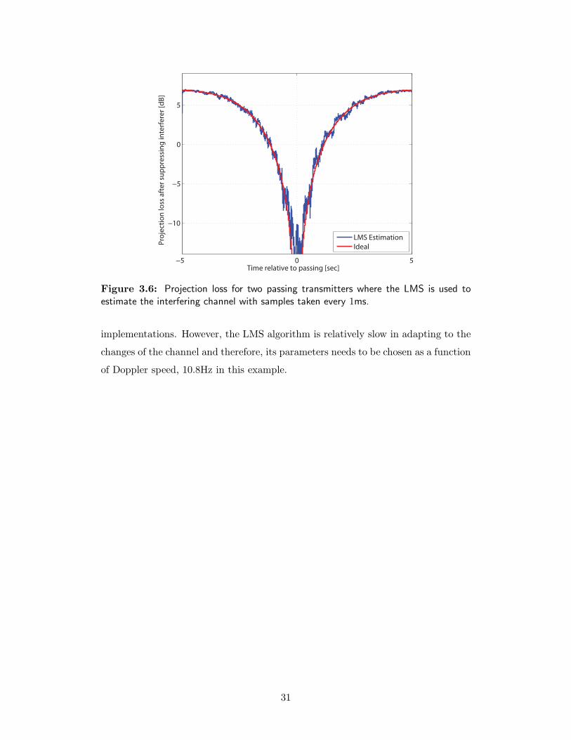
which is known as perfect CSIR. However, Fig. 3.6 represents the projection loss

due to null-steering when the channel is estimated by the LMS algorithm. This also

verifies that LMS algorithm is a suitable tool for channel estimation in practical

30

−5 0 5

−10

−5

0

5

Time relative to passing [sec]

Pro

ject

ion

loss

aft

er

sup

pre

ssin

g in

terf

ere

r [d

B]

LMS Estimation

Ideal

Figure 3.6: Projection loss for two passing transmitters where the LMS is used toestimate the interfering channel with samples taken every 1ms.

implementations. However, the LMS algorithm is relatively slow in adapting to the

changes of the channel and therefore, its parameters needs to be chosen as a function

of Doppler speed, 10.8Hz in this example.

31

Chapter 4

Channel State InformationFeedback and Quantization

Knowledge of the parameters of the wireless channel at the transmitter side is cru-

cial for establishing reliable communication at rates close to the channel capacity.

Changes in the channel response caused by mobility of the transmitter and receiver

and evolution of the signal propagation environment require adaptation of the trans-

mission strategy. Knowledge of the channel state information (CSI) obtained by the

receiver using channel estimation techniques needs to be communicated back to the

transmitter via a feedback channel. Due to errors in channel estimation and the

limitations of the feedback channel, the transmitter often needs to operate in the

presence of imperfect CSI. This is particulary important for communications over

multiple antenna channels where transmission can be very sensitive to CSI errors.

4.1 Finite-Rate Feedback of CSI

The concept of channels with feedback was introduced by Shannon [26] and an enor-

mous amount of research effort has been dedicated to applications of this concept

to various wireless communication systems. Although the capacity of the feedback

channel remains unknown for the general case, feedback is widely used in practi-

cal communications. Particularly, in 3G and 4G cellular standards feedback of the

signal-to-interference and noise ratio (SINR) conditions of the mobile station is used

for rate adaptation at the transmitter and even feedback of information about the

channel matrix is used for transmission in MIMO modes.

Cellular networks with a single-antenna BS achieve their highest throughput us-

ing scheduling techniques, where each MS is required to feed back its SINR condition

32

to the BS. In order to reduce the feedback traffic on the uplink channel, applying a

predetermined threshold for sending back the SINR condition has been proposed [27]

together, with a large number of other user selection algorithms considering limited

feedback and targeting optimization of various quality parameters. Shared feedback

resources were first studied in [28] which considers a shared random access feedback

channel. Also, in [29], another technique where users can compete for resources in

a limited feedback channel is discussed. A number of theoretic results for channels

with limited feedback have been obtained. For example, in [30] the capacity of a

broadcast channel with finite-rate feedback is computed.

For cellular networks with multiple antennas at the BS, single user (opportunis-

tic) or multiuser MIMO (MU-MIMO) downlink transmission can be utilized and

antenna array gains can be expected; see Section 1.2. Efficient communication over

MIMO channels requires knowledge of the channel matrix at the transmitter; see

Section 1.2. Particularly this knowledge is required for the optimal power alloca-

tion scenario that maximizes the mutual information of the MIMO channel and is

achieved through waterfilling over the channel singular values [31]. Linear precod-

ing methods, including beamforming, require transmitter channel state information

(CSIT) as well. Similarly, efficient operation in the MU-MIMO scenario happens

primarily when precoding is applied at the BS to minimize the cross-interference

between the data streams directed to the MS users. Due to the limitations of the

feedback channel, CSI feedback is mostly accomplished in a quantized form where

the receiver approximates the channel vector (for single-antenna MS) by a codeword

from a codebook, which is known to both transmitter and receiver [32]. The index

of the codeword is then communicated from the receiver to the transmitter via the

feedback link.

One of the fundamental research questions is to quantify the throughput loss

which is experienced by a system using quantized CSI feedback to the ideal theoretic

case of full CSI. The amount of quantization and feedback is quantified in terms of

the number of quantization bits. It has been shown that even a small amount of

feedback is proven to be beneficial [33, 34] and provides sizable gains over no-CSI

cases. However, [32] demonstrated that the number of feedback bits should be on the

order of the number of transmit antennas M at the BS and log(SINR) experienced

by MS users to maintain a constant gap between the sum-rate of the ideal CSIT case

and the realistic case with quantization. Section 4.2 discusses the above problem in

33

detail and illustrates theoretic results.

Evidently, the choice of quantization methods also affects the performance of

the quantized system. Many techniques have been proposed for quantization of

the channel vectors; among these are the random vector quantization (RVQ) and

Grassmannian line packing [35]; see Section 4.3. We also note that channel esti-

mation at the receiver side is not error-free; there are also delays in feeding back

the CSI information. Therefore, a significant number of research contributions have

been dedicated to designing codebooks and analyzing, and to frequency of the CSI

feedback. Section 4.4.1 discusses joint channel estimation and quantized feedback.

4.2 Feedback Quantization for Multiuser MIMO, Prob-

lem Definition and Approach

Channel state information in flat fading MIMO channels consists of two components

(a) Channel quality information (CQI), which carries the information regarding the

channel’s SINR, and (b) Channel direction information (CDI), which carries the

information regarding the direction of the channel vector.

In the present discussion we limit our consideration to quantization and feedback

of CDI assuming perfect knowledge of CQI. We consider the downlink communica-

tion scenario and assume that the BS is equipped with M antennas and is sending

K ≤ M independent data streams to K users. Each MS is equipped with a single

antenna. It has been shown in [30] that in the case a BS that is serving a number

of MSs that is smaller than or equal to the number of transmit antennas at the BS,

the knowledge of the magnitude of CSI is not required.

Let the composite downlink channel matrix be

H† = [h1 h2 · · · hK ]

where H has dimension K ×M . The signal received by the ith MS is

yi = h†ix+ ηi, i = 1, 2, . . . ,K (4.1)

where hi ∈ CM×1 and x ∈ CM×1 is the transmitted signal. We consider linear

precoding where the transmitter multiplies the symbol intended for each user (MS)

by a beamforming vector and transmits the sum of these vectors to the users. Let

us denote the symbol intended for the ith user by si and the corresponding unit

34

norm beamforming vector by νi. Then the transmitted signal is

x =K∑

i=1

siνi

and therefore, the signal (4.1) received by the ith user is

yi = h†ix+ ηi = h†

i

K∑

i=1

siνi + ηi.

Typically ZF beamforming is used as the precoding scheme, meaning that the

beamforming vectors νi are chosen to be the normalized columns of H∗(HH∗)−1

(see 1.2). The precoding matrix is designed to orthogonalize the signals transmitted

to the users. However, this orthogonalization cannot be perfect since the knowledge

of channel matrixH† is incomplete: information sent from MS to BS via the feedback

channel must be quantized and therefore carries inherent quantization errors. We

assume that the BS has obtained an estimate H of the matrix H. This estimate is

formed by K vectors hi received via feedback from the K users. We assume that

ith MS uses Bi bits to quantize its 1×M channel vector h†i .

Let us consider the Rayleigh fading channel H and assume that random vector

quantization is performed at every MS to quantize the channel information. It has

been shown in [32] that for random vector quantization of Gaussian vectors, the

average quantization error is upper bounded as

EH,W

[

sin2(

∠

(

hi, hi

))]

< 2−Bi

M−1 . (4.2)

where hi =hi

‖hi‖ and the expectation is taken over the channel realizations and the

quantization codebooks.

We make the assumption that Pti is the allocated signal power on the data stream

transmitted to the ith MS. The SINR at the ith MS (see (4.1)) can be evaluated as:

SINRi =Pti |h†

iνi|2

1 +∑

j 6=i Ptj |h†iνj |2

. (4.3)

We assume that precoding vectors νi are the columns of the ZF beamforming ma-

trix H∗(HH∗)−1 constructed using quantized channel matrix H†. It has been shown

in [32] that the residual interference terms in the denominator of (4.3) can be up-

perbounded as

EH,W

[

sin2(

∠

(

hi, νj

))]

< 2−Bi

M−1 . (4.4)

35

We now compare the sum-rate capacity of the ideal ZF beamforming case and

the sum-rate with ZF beamforming based on quantized feedback information. We

follow the lines of derivation in [32] but consider the unequal power case. The

sum-rate for the ideal ZF case is equal to

RZF (Pt1 , . . . Ptk , B1, . . . Bk) =

K∑

i=1

EH

[

log2

(

1 + Pti |h†iνZF,i|2

)]

where νZF,i is orthogonal to hj , j 6= i. The rate for the quantized case is

RFB (Pt1 , . . . PtK , B1, . . . BK) =

K∑

i=1

EH,W [log2 (1 + SINRi)]

=

K∑

i=1

EH,W

[

log2

(

1 +Pti |h

†iνi|2

1 +∑

j 6=i Ptj |h†iνj |2

)]

=

K∑

i=1

EH,W

log2

1 + Pti |h†iνi|2 +

∑

j 6=i

Pti |h†iνj |2

+K∑

i=1

EH,W

log2

1 +∑

j 6=i

Pti |h†iνj |2

≤K∑

i=1

EH,W

[

log2

(

1 + Pti |h†iνi|2

)]

+K∑

i=1

EH,W

log2

1 +∑

j 6=i

Pti |h†iνj |2

We start upper bounding the difference between rates

∆R(Pt1 , . . . PtK , B1, . . . BK) = RZF (Pt1 , . . . PtK , B1, . . . BK)

−RFB (Pt1 , . . . PtK , B1, . . . BK)

≤K∑

i=1

EH,W

log2

1 +∑

j 6=i

Ptj |h†iνj |2

observing that

EH

[

log2

(

1 + Pti |h†iνZF,i|2

)]

= EH,W

[

log2

(

1 + Pti |h†iνi|2

)]

.

Using (4.2), (4.4), and Jensen’s inequality assuming E(‖hk‖2

)=M , we obtain

∆R (Pt1 , . . . PtK , B1, . . . Bk) ≤K∑

i=1

log2

(

1 +M

M − 1Pti2

− BiM−1

)

(4.5)

36

1√2

1√2

0 1√2e2πj/3

1√2

0 1√2

1√2e4πj/3

0 1√2

1√2

0

1√2e2πj/3 1√

2e4πj/3 1√

2e4πj/3 0

0 0 1√2e2πj/3 1√

2e4πj/3

1√2e4πj/3 1√

2e2πj/3 0 1√

2e2πj/3

Table 4.1: Grassmannian generated codebook for M = 3 and N = 23 = 8.

For the case of equal power data streams, i.e. Pti = Pt/M , i = 1, 2, . . . ,K, and the

numbers of bits Bi = B, i = 1, 2, . . . ,K (4.5) simplifies to

∆R (Pt, . . . Pt, B, . . . B) ≤ K log2

(

1 +M

M − 1Pt2

− BM−1

)

(4.6)

and leads to the formula for the number of bits [32]

B = (M − 1) log(Pt, 2) ≈M − 1

3PtdB (4.7)

required to get a constant gap between the ideal and quantized performances. In

the case where the fixed number of bits B is used the SINRi values will saturate at

some constant level, as can be seen from (4.3).

Looking at (4.5) we notice that in order to balance the terms on the right hand

side (i.e., making them equal) we need

Pti 2− Bi

M−1 ≈ Ptj 2−Bj

M−1 i 6= j (4.8)

This means that users with smaller SINR need fewer feedback bits and users with

higher SINR need more bits to maintain the same scaling of the gap from the ideal

ZF beamforming rate.

4.3 Codebook Design

Codebook design is an important component in feedback quantization. Quantization

error can be reduced by increasing the codebook size. As a result, optimal, perfect

CSI performance can be approached at the cost of compromising data transmission

rate in the opposite direction. Feedback information itself becomes sensitive to errors

if the amount of feedback bits is increased significantly. Therefore, it is essential not

to use an excessively high feedback rate to optimize a system’s performance [36].

37

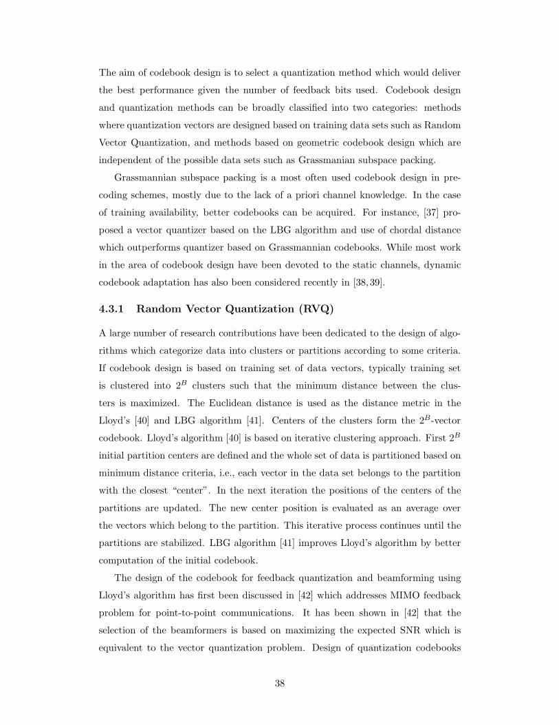
The aim of codebook design is to select a quantization method which would deliver

the best performance given the number of feedback bits used. Codebook design

and quantization methods can be broadly classified into two categories: methods

where quantization vectors are designed based on training data sets such as Random

Vector Quantization, and methods based on geometric codebook design which are

independent of the possible data sets such as Grassmanian subspace packing.

Grassmannian subspace packing is a most often used codebook design in pre-

coding schemes, mostly due to the lack of a priori channel knowledge. In the case

of training availability, better codebooks can be acquired. For instance, [37] pro-

posed a vector quantizer based on the LBG algorithm and use of chordal distance

which outperforms quantizer based on Grassmannian codebooks. While most work

in the area of codebook design have been devoted to the static channels, dynamic

codebook adaptation has also been considered recently in [38,39].

4.3.1 Random Vector Quantization (RVQ)

A large number of research contributions have been dedicated to the design of algo-

rithms which categorize data into clusters or partitions according to some criteria.

If codebook design is based on training set of data vectors, typically training set

is clustered into 2B clusters such that the minimum distance between the clus-

ters is maximized. The Euclidean distance is used as the distance metric in the

Lloyd’s [40] and LBG algorithm [41]. Centers of the clusters form the 2B-vector

codebook. Lloyd’s algorithm [40] is based on iterative clustering approach. First 2B

initial partition centers are defined and the whole set of data is partitioned based on

minimum distance criteria, i.e., each vector in the data set belongs to the partition

with the closest “center”. In the next iteration the positions of the centers of the

partitions are updated. The new center position is evaluated as an average over

the vectors which belong to the partition. This iterative process continues until the

partitions are stabilized. LBG algorithm [41] improves Lloyd’s algorithm by better

computation of the initial codebook.

The design of the codebook for feedback quantization and beamforming using

Lloyd’s algorithm has first been discussed in [42] which addresses MIMO feedback

problem for point-to-point communications. It has been shown in [42] that the

selection of the beamformers is based on maximizing the expected SNR which is

equivalent to the vector quantization problem. Design of quantization codebooks

38

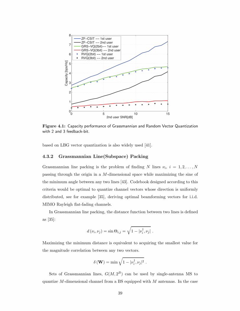
0 5 10 150

1

2

3

4

5

6

7

8

2nd user SNR[dB]

Ca

pa

city [b

ps/H

z]

ZF−CSIT −− 1st user

ZF−CSIT −− 2nd user

GRS−VQ(2bit)−− 1st userGRS−VQ(3bit) −− 2nd user

RVQ(2bit) −− 1st user

RVQ(3bit) −− 2nd user

Figure 4.1: Capacity performance of Grassmannian and Random Vector Quantizationwith 2 and 3 feedback-bit.

based on LBG vector quantization is also widely used [41].

4.3.2 Grassmannian Line(Subspace) Packing

Grassmannian line packing is the problem of finding N lines νi, i = 1, 2, . . . , N

passing through the origin in a M -dimensional space while maximizing the sine of

the minimum angle between any two lines [43]. Codebook designed according to this

criteria would be optimal to quantize channel vectors whose direction is uniformly

distributed, see for example [35], deriving optimal beamforming vectors for i.i.d.

MIMO Rayleigh flat-fading channels.

In Grassmannian line packing, the distance function between two lines is defined

as [35]:

d (νi, νj) = sinΘi,j =

√

1− |ν†i , νj | .

Maximizing the minimum distance is equivalent to acquiring the smallest value for

the magnitude correlation between any two vectors.

δ (W) = min

√

1− |ν†i , νj |2 .

Sets of Grassmannian lines, G(M, 2B) can be used by single-antenna MS to

quantize M -dimensional channel from a BS equipped with M antennas. In the case

39

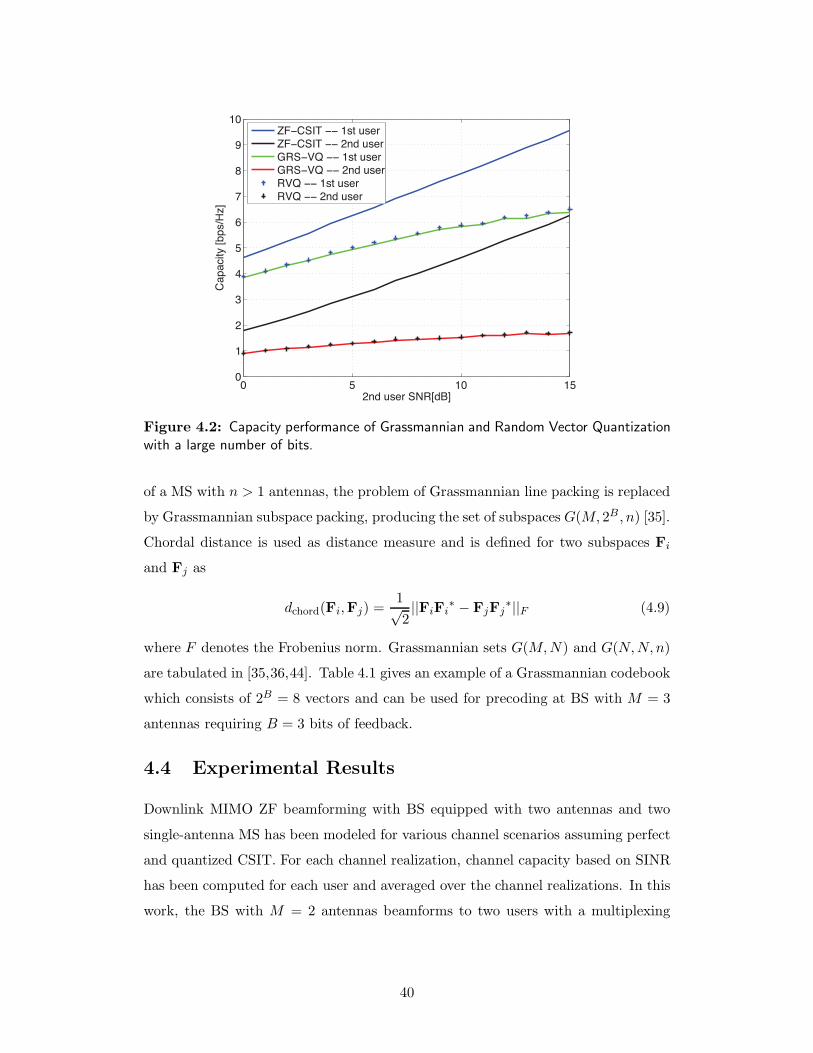
0 5 10 150

1

2

3

4

5

6

7

8

9

10

2nd user SNR[dB]

Ca

pa

city [b

ps/H

z]

ZF−CSIT −− 1st user

ZF−CSIT −− 2nd user

GRS−VQ −− 1st userGRS−VQ −− 2nd user

RVQ −− 1st user

RVQ −− 2nd user

Figure 4.2: Capacity performance of Grassmannian and Random Vector Quantizationwith a large number of bits.

of a MS with n > 1 antennas, the problem of Grassmannian line packing is replaced

by Grassmannian subspace packing, producing the set of subspaces G(M, 2B , n) [35].

Chordal distance is used as distance measure and is defined for two subspaces Fi

and Fj as

dchord(Fi,Fj) =1√2||FiFi

∗ − FjFj∗||F (4.9)

where F denotes the Frobenius norm. Grassmannian sets G(M,N) and G(N,N, n)

are tabulated in [35,36,44]. Table 4.1 gives an example of a Grassmannian codebook

which consists of 2B = 8 vectors and can be used for precoding at BS with M = 3

antennas requiring B = 3 bits of feedback.

4.4 Experimental Results

Downlink MIMO ZF beamforming with BS equipped with two antennas and two

single-antenna MS has been modeled for various channel scenarios assuming perfect

and quantized CSIT. For each channel realization, channel capacity based on SINR

has been computed for each user and averaged over the channel realizations. In this

work, the BS with M = 2 antennas beamforms to two users with a multiplexing

40

8 10 12 14 16 18 200

1

2

3

4

5

6

Power[dB] for strong user

Ca

pa

city [b

ps/H

z]

ZF−CSIT−user1

ZF−CSIT−user2

RVQ−user1RVQ−user2

fixed−bits (5 bits)

fixed−bits (3 bits)

Figure 4.3: Capacity performance of Grassmannian and Random Vector Quantizationwith a constant number of feedback bits.

transmission scheme. The power allocation is applied before data transmission

[y1y2

]

= HG

[Pt1 00 Pt2

] [d1d2

]

+

[n1n2

]

.

Fig. 4.1 displays the capacity performance for Rayleigh channel case where the

transmit power allocated for the first user is 10dB higher than the power allocated

for the second user. The results are plotted as a function of the 2nd user’s SNR.

Capacity for the 1st user (blue curve) and the 2nd user (black curve) assuming ideal

CSIT are shown by the solid lines as well as capacity for the 1st user (green curve)

and the 2nd user (red curve) assuming Grassmanian vector quantization with 2 and

3 feedback bits, respectively. Finally, the capacities of the 1st user (dotted blue)

and 2nd user (dotted black) assuming random vector quantization with 2 and 3

feedback bits respectively, are also demonstrated. Note that this result is obtained

from averaging the capacity performance of over 10000 channel coefficients. It can be

observed that quantization with a fixed number of bits is not sufficient to maintain

a fixed gap between quantized and ideal capacity performance. We can also notice

that Grassmanian design outperforms RVQ for this case since Grassmanian vectors

are optimal for the Rayleigh channel case.

Fig. 4.2 displays the capacity performance for the same setup as Fig. 4.1, how-

ever, a BS with 4 antennas is considered and each of two users has a single antenna.

41

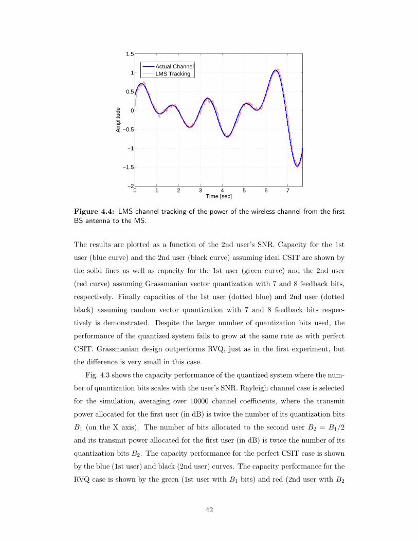
0 1 2 3 4 5 6 7−2

−1.5

−1

−0.5

0

0.5

1

1.5

Time [sec]

Am

plitu

de

Actual ChannelLMS Tracking

Figure 4.4: LMS channel tracking of the power of the wireless channel from the firstBS antenna to the MS.

The results are plotted as a function of the 2nd user’s SNR. Capacity for the 1st

user (blue curve) and the 2nd user (black curve) assuming ideal CSIT are shown by

the solid lines as well as capacity for the 1st user (green curve) and the 2nd user

(red curve) assuming Grassmanian vector quantization with 7 and 8 feedback bits,

respectively. Finally capacities of the 1st user (dotted blue) and 2nd user (dotted

black) assuming random vector quantization with 7 and 8 feedback bits respec-

tively is demonstrated. Despite the larger number of quantization bits used, the

performance of the quantized system fails to grow at the same rate as with perfect

CSIT. Grassmanian design outperforms RVQ, just as in the first experiment, but

the difference is very small in this case.

Fig. 4.3 shows the capacity performance of the quantized system where the num-

ber of quantization bits scales with the user’s SNR. Rayleigh channel case is selected

for the simulation, averaging over 10000 channel coefficients, where the transmit

power allocated for the first user (in dB) is twice the number of its quantization bits

B1 (on the X axis). The number of bits allocated to the second user B2 = B1/2

and its transmit power allocated for the first user (in dB) is twice the number of its

quantization bits B2. The capacity performance for the perfect CSIT case is shown

by the blue (1st user) and black (2nd user) curves. The capacity performance for the

RVQ case is shown by the green (1st user with B1 bits) and red (2nd user with B2

42

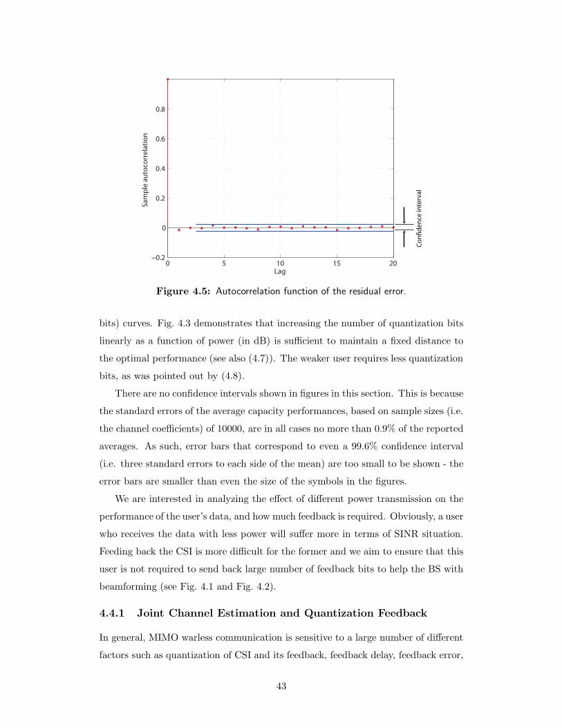
0 5 10 15 20−0.2

0

0.2

0.4

0.6

0.8

Lag

Sample autocorrelation

Co

n�

de

nce

inte

rva

l

Figure 4.5: Autocorrelation function of the residual error.

bits) curves. Fig. 4.3 demonstrates that increasing the number of quantization bits

linearly as a function of power (in dB) is sufficient to maintain a fixed distance to

the optimal performance (see also (4.7)). The weaker user requires less quantization

bits, as was pointed out by (4.8).

There are no confidence intervals shown in figures in this section. This is because

the standard errors of the average capacity performances, based on sample sizes (i.e.

the channel coefficients) of 10000, are in all cases no more than 0.9% of the reported

averages. As such, error bars that correspond to even a 99.6% confidence interval

(i.e. three standard errors to each side of the mean) are too small to be shown - the

error bars are smaller than even the size of the symbols in the figures.

We are interested in analyzing the effect of different power transmission on the

performance of the user’s data, and how much feedback is required. Obviously, a user

who receives the data with less power will suffer more in terms of SINR situation.

Feeding back the CSI is more difficult for the former and we aim to ensure that this

user is not required to send back large number of feedback bits to help the BS with

beamforming (see Fig. 4.1 and Fig. 4.2).

4.4.1 Joint Channel Estimation and Quantization Feedback

In general, MIMO warless communication is sensitive to a large number of different

factors such as quantization of CSI and its feedback, feedback delay, feedback error,

43

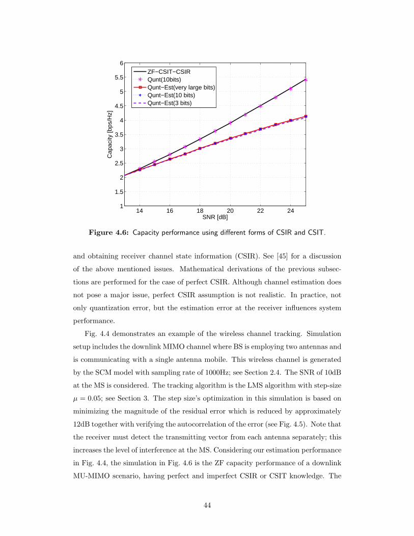
14 16 18 20 22 241

1.5

2

2.5

3

3.5

4

4.5

5

5.5

6

SNR [dB]

Cap

acity

[bps

/Hz]

ZF−CSIT−CSIRQunt(10bits)Qunt−Est(very large bits)Qunt−Est(10 bits)Qunt−Est(3 bits)

Figure 4.6: Capacity performance using different forms of CSIR and CSIT.

and obtaining receiver channel state information (CSIR). See [45] for a discussion

of the above mentioned issues. Mathematical derivations of the previous subsec-

tions are performed for the case of perfect CSIR. Although channel estimation does

not pose a major issue, perfect CSIR assumption is not realistic. In practice, not

only quantization error, but the estimation error at the receiver influences system

performance.

Fig. 4.4 demonstrates an example of the wireless channel tracking. Simulation

setup includes the downlink MIMO channel where BS is employing two antennas and

is communicating with a single antenna mobile. This wireless channel is generated

by the SCM model with sampling rate of 1000Hz; see Section 2.4. The SNR of 10dB

at the MS is considered. The tracking algorithm is the LMS algorithm with step-size

µ = 0.05; see Section 3. The step size’s optimization in this simulation is based on

minimizing the magnitude of the residual error which is reduced by approximately

12dB together with verifying the autocorrelation of the error (see Fig. 4.5). Note that

the receiver must detect the transmitting vector from each antenna separately; this

increases the level of interference at the MS. Considering our estimation performance

in Fig. 4.4, the simulation in Fig. 4.6 is the ZF capacity performance of a downlink

MU-MIMO scenario, having perfect and imperfect CSIR or CSIT knowledge. The

44

BS includes two antennas, multiplexing data to two users. This result indicates that

when the estimation error is not negligible, the ZF capacity assuming perfect CSIT

and CSIR (black curve) experiences performance degradation (red curve).

Assuming perfect CSIR, increasing the number of feedback bits leads to capacity

growth (pink curve); see Section 4.2. However, with the non-negligible estimation

error (imperfect CSIR), increasing the number of feedback bits does not change

the capacity performance. It can be observed from Fig. 4.6 that 3-bit and 10-bit

feedback quantization converge to same capacity as infinite number of feedback

bits. A natural conclusion from the observed performance is that the number of

quantization bits needs to be selected in correspondence of the channel estimation

quality.

45

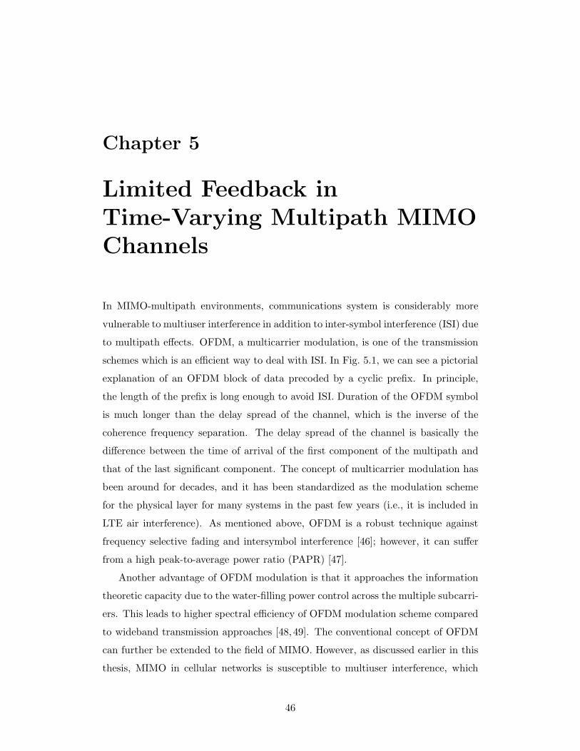
Chapter 5

Limited Feedback inTime-Varying Multipath MIMOChannels

In MIMO-multipath environments, communications system is considerably more

vulnerable to multiuser interference in addition to inter-symbol interference (ISI) due

to multipath effects. OFDM, a multicarrier modulation, is one of the transmission

schemes which is an efficient way to deal with ISI. In Fig. 5.1, we can see a pictorial

explanation of an OFDM block of data precoded by a cyclic prefix. In principle,

the length of the prefix is long enough to avoid ISI. Duration of the OFDM symbol

is much longer than the delay spread of the channel, which is the inverse of the

coherence frequency separation. The delay spread of the channel is basically the

difference between the time of arrival of the first component of the multipath and

that of the last significant component. The concept of multicarrier modulation has

been around for decades, and it has been standardized as the modulation scheme

for the physical layer for many systems in the past few years (i.e., it is included in

LTE air interference). As mentioned above, OFDM is a robust technique against

frequency selective fading and intersymbol interference [46]; however, it can suffer

from a high peak-to-average power ratio (PAPR) [47].

Another advantage of OFDM modulation is that it approaches the information

theoretic capacity due to the water-filling power control across the multiple subcarri-

ers. This leads to higher spectral efficiency of OFDM modulation scheme compared

to wideband transmission approaches [48, 49]. The conventional concept of OFDM

can further be extended to the field of MIMO. However, as discussed earlier in this

thesis, MIMO in cellular networks is susceptible to multiuser interference, which

46

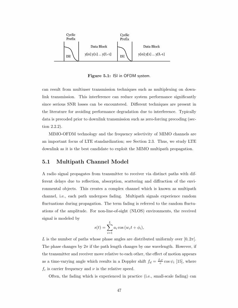
Figure 5.1: ISI in OFDM system.

can result from multiuser transmission techniques such as multiplexing on down-

link transmission. This interference can reduce system performance significantly

since serious SNR losses can be encountered. Different techniques are present in

the literature for avoiding performance degradation due to interference. Typically

data is precoded prior to downlink transmission such as zero-forcing precoding (sec-

tion 2.2.2).

MIMO-OFDM technology and the frequency selectivity of MIMO channels are

an important focus of LTE standardization; see Section 2.3. Thus, we study LTE

downlink as it is the best candidate to exploit the MIMO multipath propagation.

5.1 Multipath Channel Model

A radio signal propagates from transmitter to receiver via distinct paths with dif-

ferent delays due to reflection, absorption, scattering and diffraction of the envi-

ronmental objects. This creates a complex channel which is known as multipath

channel, i.e., each path undergoes fading. Multipath signals experience random

fluctuations during propagation. The term fading is referred to the random fluctu-

ations of the amplitude. For non-line-of-sight (NLOS) environments, the received

signal is modeled by

s(t) =

L∑

i=1

ai cos (wct+ φi),

L is the number of paths whose phase angles are distributed uniformly over [0, 2π].

The phase changes by 2π if the path length changes by one wavelength. However, if

the transmitter and receiver move relative to each other, the effect of motion appears

as a time-varying angle which results in a Doppler shift fd = fcνc cosψi [15], where

fc is carrier frequency and ν is the relative speed.

Often, the fading which is experienced in practice (i.e., small-scale fading) can

47

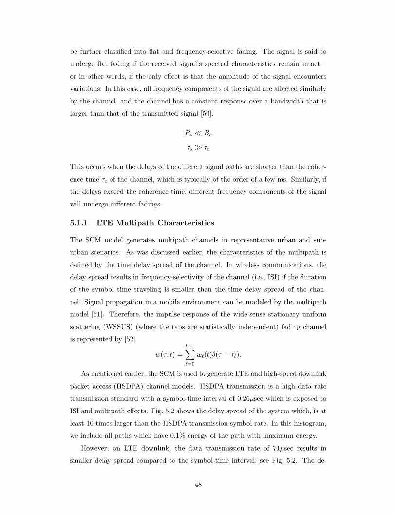
be further classified into flat and frequency-selective fading. The signal is said to

undergo flat fading if the received signal’s spectral characteristics remain intact –

or in other words, if the only effect is that the amplitude of the signal encounters

variations. In this case, all frequency components of the signal are affected similarly

by the channel, and the channel has a constant response over a bandwidth that is

larger than that of the transmitted signal [50].

Bs ≪ Bc

τs ≫ τc

This occurs when the delays of the different signal paths are shorter than the coher-

ence time τc of the channel, which is typically of the order of a few ms. Similarly, if

the delays exceed the coherence time, different frequency components of the signal

will undergo different fadings.

5.1.1 LTE Multipath Characteristics

The SCM model generates multipath channels in representative urban and sub-

urban scenarios. As was discussed earlier, the characteristics of the multipath is

defined by the time delay spread of the channel. In wireless communications, the

delay spread results in frequency-selectivity of the channel (i.e., ISI) if the duration

of the symbol time traveling is smaller than the time delay spread of the chan-

nel. Signal propagation in a mobile environment can be modeled by the multipath

model [51]. Therefore, the impulse response of the wide-sense stationary uniform

scattering (WSSUS) (where the taps are statistically independent) fading channel

is represented by [52]

w(τ, t) =

L−1∑

ℓ=0

wℓ(t)δ(τ − τℓ).

As mentioned earlier, the SCM is used to generate LTE and high-speed downlink

packet access (HSDPA) channel models. HSDPA transmission is a high data rate

transmission standard with a symbol-time interval of 0.26µsec which is exposed to

ISI and multipath effects. Fig. 5.2 shows the delay spread of the system which, is at

least 10 times larger than the HSDPA transmission symbol rate. In this histogram,

we include all paths which have 0.1% energy of the path with maximum energy.

However, on LTE downlink, the data transmission rate of 71µsec results in

smaller delay spread compared to the symbol-time interval; see Fig. 5.2. The de-

48

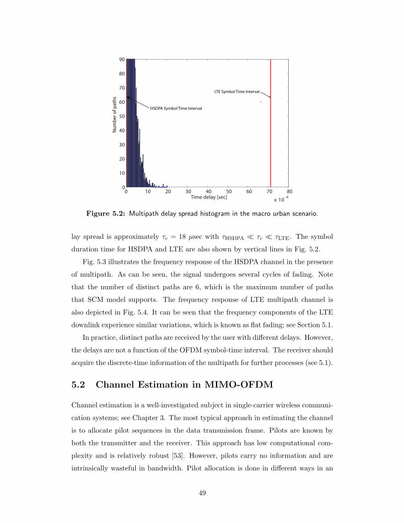
0 10 20 30 40 50 60 70 80

x 10−6

0

10

20

30

40

50

60

70

80

90

Time delay [sec]

LTE Symbol Time Interval

HSDPA Symbol Time Interval

Nu

mb

er

of

pa

ths

Figure 5.2: Multipath delay spread histogram in the macro urban scenario.

lay spread is approximately τc = 18 µsec with τHSDPA ≪ τc ≪ τLTE. The symbol

duration time for HSDPA and LTE are also shown by vertical lines in Fig. 5.2.

Fig. 5.3 illustrates the frequency response of the HSDPA channel in the presence

of multipath. As can be seen, the signal undergoes several cycles of fading. Note

that the number of distinct paths are 6, which is the maximum number of paths

that SCM model supports. The frequency response of LTE multipath channel is

also depicted in Fig. 5.4. It can be seen that the frequency components of the LTE

downlink experience similar variations, which is known as flat fading; see Section 5.1.

In practice, distinct paths are received by the user with different delays. However,

the delays are not a function of the OFDM symbol-time interval. The receiver should

acquire the discrete-time information of the multipath for further processes (see 5.1).

5.2 Channel Estimation in MIMO-OFDM

Channel estimation is a well-investigated subject in single-carrier wireless communi-

cation systems; see Chapter 3. The most typical approach in estimating the channel

is to allocate pilot sequences in the data transmission frame. Pilots are known by

both the transmitter and the receiver. This approach has low computational com-

plexity and is relatively robust [53]. However, pilots carry no information and are

intrinsically wasteful in bandwidth. Pilot allocation is done in different ways in an

49

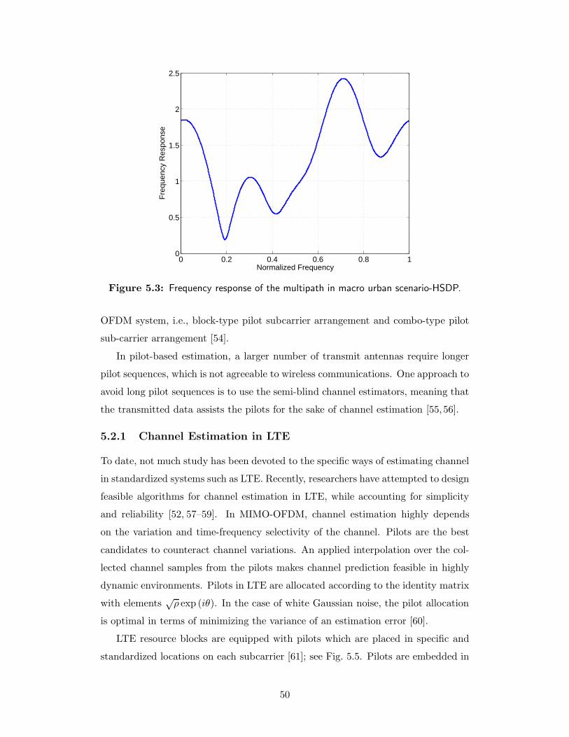
0 0.2 0.4 0.6 0.8 10

0.5

1

1.5

2

2.5

Normalized Frequency

Fre

quen

cy R

espo

nse

Figure 5.3: Frequency response of the multipath in macro urban scenario-HSDP.

OFDM system, i.e., block-type pilot subcarrier arrangement and combo-type pilot

sub-carrier arrangement [54].

In pilot-based estimation, a larger number of transmit antennas require longer

pilot sequences, which is not agreeable to wireless communications. One approach to

avoid long pilot sequences is to use the semi-blind channel estimators, meaning that

the transmitted data assists the pilots for the sake of channel estimation [55,56].

5.2.1 Channel Estimation in LTE

To date, not much study has been devoted to the specific ways of estimating channel

in standardized systems such as LTE. Recently, researchers have attempted to design

feasible algorithms for channel estimation in LTE, while accounting for simplicity

and reliability [52, 57–59]. In MIMO-OFDM, channel estimation highly depends

on the variation and time-frequency selectivity of the channel. Pilots are the best

candidates to counteract channel variations. An applied interpolation over the col-

lected channel samples from the pilots makes channel prediction feasible in highly

dynamic environments. Pilots in LTE are allocated according to the identity matrix

with elements√ρ exp (iθ). In the case of white Gaussian noise, the pilot allocation

is optimal in terms of minimizing the variance of an estimation error [60].

LTE resource blocks are equipped with pilots which are placed in specific and

standardized locations on each subcarrier [61]; see Fig. 5.5. Pilots are embedded in

50

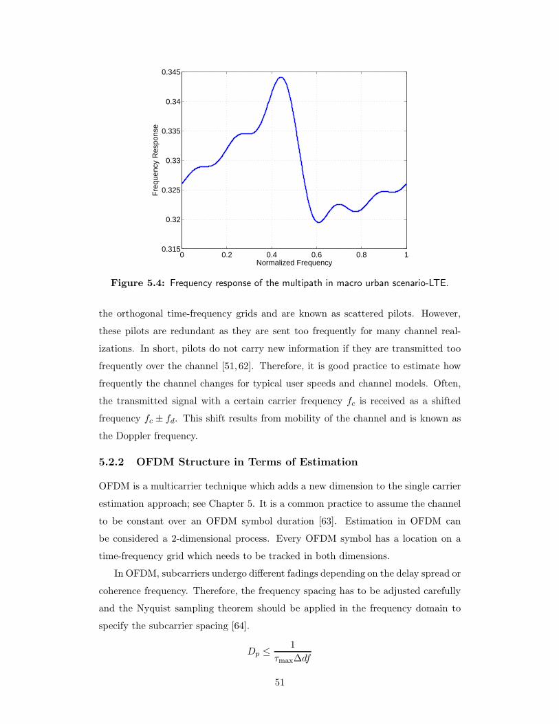
0 0.2 0.4 0.6 0.8 10.315

0.32

0.325

0.33

0.335

0.34

0.345

Normalized Frequency

Fre

quen

cy R

espo

nse

Figure 5.4: Frequency response of the multipath in macro urban scenario-LTE.

the orthogonal time-frequency grids and are known as scattered pilots. However,

these pilots are redundant as they are sent too frequently for many channel real-

izations. In short, pilots do not carry new information if they are transmitted too

frequently over the channel [51, 62]. Therefore, it is good practice to estimate how

frequently the channel changes for typical user speeds and channel models. Often,

the transmitted signal with a certain carrier frequency fc is received as a shifted

frequency fc ± fd. This shift results from mobility of the channel and is known as

the Doppler frequency.

5.2.2 OFDM Structure in Terms of Estimation

OFDM is a multicarrier technique which adds a new dimension to the single carrier

estimation approach; see Chapter 5. It is a common practice to assume the channel

to be constant over an OFDM symbol duration [63]. Estimation in OFDM can

be considered a 2-dimensional process. Every OFDM symbol has a location on a

time-frequency grid which needs to be tracked in both dimensions.

In OFDM, subcarriers undergo different fadings depending on the delay spread or

coherence frequency. Therefore, the frequency spacing has to be adjusted carefully

and the Nyquist sampling theorem should be applied in the frequency domain to

specify the subcarrier spacing [64].

Dp ≤1

τmax∆df

51

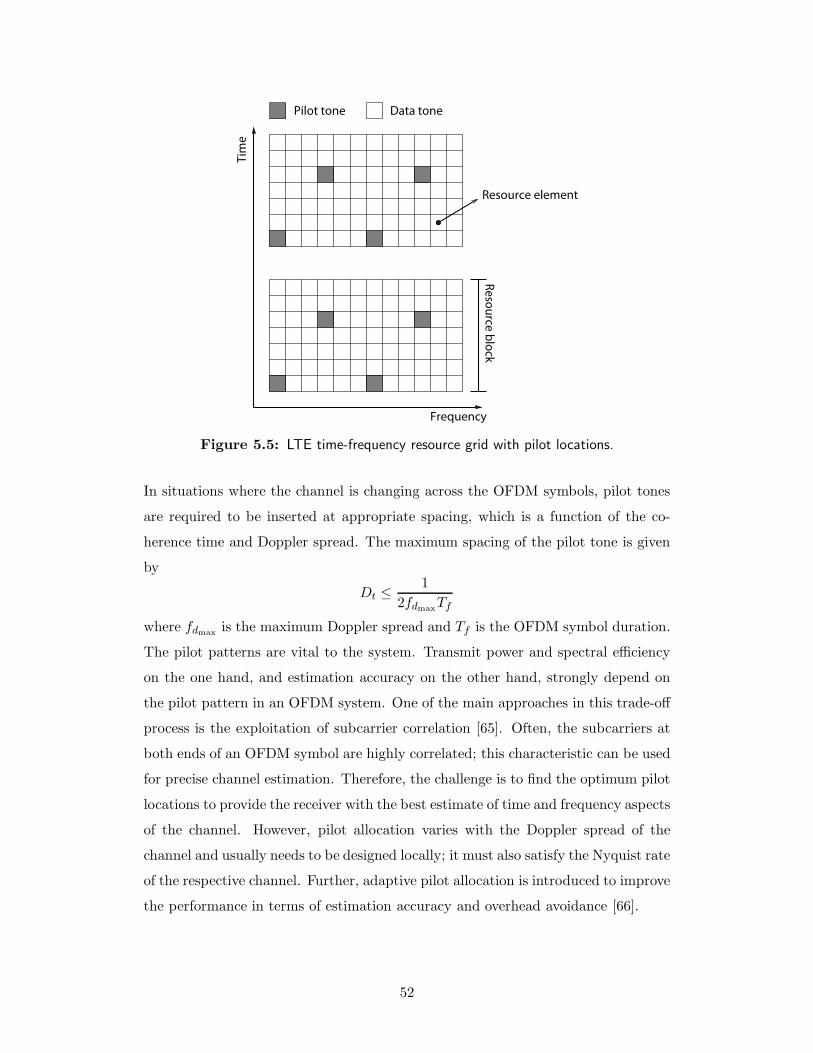
Pilot tone

Re

sou

rce b

lock

Resource element

Tim

e

Frequency

Data tone

Figure 5.5: LTE time-frequency resource grid with pilot locations.

In situations where the channel is changing across the OFDM symbols, pilot tones

are required to be inserted at appropriate spacing, which is a function of the co-

herence time and Doppler spread. The maximum spacing of the pilot tone is given

by

Dt ≤1

2fdmaxTf

where fdmaxis the maximum Doppler spread and Tf is the OFDM symbol duration.

The pilot patterns are vital to the system. Transmit power and spectral efficiency

on the one hand, and estimation accuracy on the other hand, strongly depend on

the pilot pattern in an OFDM system. One of the main approaches in this trade-off

process is the exploitation of subcarrier correlation [65]. Often, the subcarriers at

both ends of an OFDM symbol are highly correlated; this characteristic can be used

for precise channel estimation. Therefore, the challenge is to find the optimum pilot

locations to provide the receiver with the best estimate of time and frequency aspects

of the channel. However, pilot allocation varies with the Doppler spread of the

channel and usually needs to be designed locally; it must also satisfy the Nyquist rate

of the respective channel. Further, adaptive pilot allocation is introduced to improve

the performance in terms of estimation accuracy and overhead avoidance [66].

52

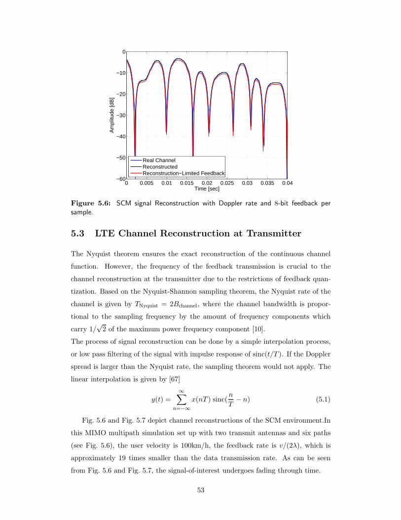
0 0.005 0.01 0.015 0.02 0.025 0.03 0.035 0.04−60

−50

−40

−30

−20

−10

0

Time [sec]

Am

plitu

de [d

B]

Real ChannelReconstructedReconstruction−Limited Feedback

Figure 5.6: SCM signal Reconstruction with Doppler rate and 8-bit feedback persample.

5.3 LTE Channel Reconstruction at Transmitter

The Nyquist theorem ensures the exact reconstruction of the continuous channel

function. However, the frequency of the feedback transmission is crucial to the

channel reconstruction at the transmitter due to the restrictions of feedback quan-

tization. Based on the Nyquist-Shannon sampling theorem, the Nyquist rate of the

channel is given by TNyquist = 2Bchannel, where the channel bandwidth is propor-

tional to the sampling frequency by the amount of frequency components which

carry 1/√2 of the maximum power frequency component [10].

The process of signal reconstruction can be done by a simple interpolation process,

or low pass filtering of the signal with impulse response of sinc(t/T ). If the Doppler

spread is larger than the Nyquist rate, the sampling theorem would not apply. The

linear interpolation is given by [67]

y(t) =∞∑

n=−∞x(nT ) sinc(

n

T− n) (5.1)

Fig. 5.6 and Fig. 5.7 depict channel reconstructions of the SCM environment.In

this MIMO multipath simulation set up with two transmit antennas and six paths

(see Fig. 5.6), the user velocity is 100km/h, the feedback rate is v/(2λ), which is

approximately 19 times smaller than the data transmission rate. As can be seen

from Fig. 5.6 and Fig. 5.7, the signal-of-interest undergoes fading through time.

53

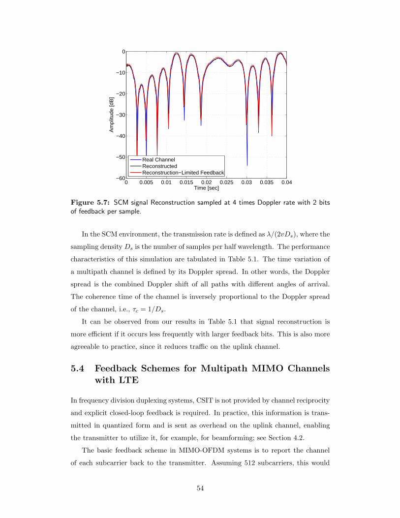
0 0.005 0.01 0.015 0.02 0.025 0.03 0.035 0.04−60

−50

−40

−30

−20

−10

0

Time [sec]

Am

plitu

de [d

B]

Real ChannelReconstructedReconstruction−Limited Feedback

Figure 5.7: SCM signal Reconstruction sampled at 4 times Doppler rate with 2 bitsof feedback per sample.

In the SCM environment, the transmission rate is defined as λ/(2vDs), where the

sampling density Ds is the number of samples per half wavelength. The performance

characteristics of this simulation are tabulated in Table 5.1. The time variation of

a multipath channel is defined by its Doppler spread. In other words, the Doppler

spread is the combined Doppler shift of all paths with different angles of arrival.

The coherence time of the channel is inversely proportional to the Doppler spread

of the channel, i.e., τc = 1/Ds.

It can be observed from our results in Table 5.1 that signal reconstruction is

more efficient if it occurs less frequently with larger feedback bits. This is also more

agreeable to practice, since it reduces traffic on the uplink channel.

5.4 Feedback Schemes for Multipath MIMO Channelswith LTE

In frequency division duplexing systems, CSIT is not provided by channel reciprocity

and explicit closed-loop feedback is required. In practice, this information is trans-

mitted in quantized form and is sent as overhead on the uplink channel, enabling

the transmitter to utilize it, for example, for beamforming; see Section 4.2.

The basic feedback scheme in MIMO-OFDM systems is to report the channel

of each subcarrier back to the transmitter. Assuming 512 subcarriers, this would

54

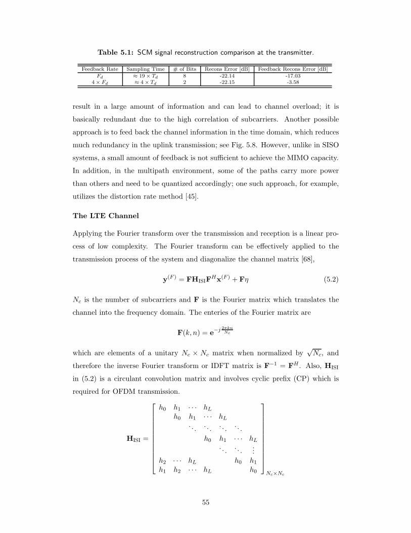
Table 5.1: SCM signal reconstruction comparison at the transmitter.

Feedback Rate Sampling Time # of Bits Recons Error [dB] Feedback Recons Error [dB]

Fd ≈ 19× Td 8 -22.14 -17.034× Fd ≈ 4× Td 2 -22.15 -3.58

result in a large amount of information and can lead to channel overload; it is

basically redundant due to the high correlation of subcarriers. Another possible

approach is to feed back the channel information in the time domain, which reduces

much redundancy in the uplink transmission; see Fig. 5.8. However, unlike in SISO

systems, a small amount of feedback is not sufficient to achieve the MIMO capacity.

In addition, in the multipath environment, some of the paths carry more power

than others and need to be quantized accordingly; one such approach, for example,

utilizes the distortion rate method [45].

The LTE Channel

Applying the Fourier transform over the transmission and reception is a linear pro-

cess of low complexity. The Fourier transform can be effectively applied to the

transmission process of the system and diagonalize the channel matrix [68],

y(F ) = FHISIFHx(F ) + Fη (5.2)

Nc is the number of subcarriers and F is the Fourier matrix which translates the

channel into the frequency domain. The enteries of the Fourier matrix are

F(k, n) = e−j 2πknNc

which are elements of a unitary Nc × Nc matrix when normalized by√Nc, and

therefore the inverse Fourier transform or IDFT matrix is F−1 = FH . Also, HISI

in (5.2) is a circulant convolution matrix and involves cyclic prefix (CP) which is

required for OFDM transmission.

HISI =

h0 h1 · · · hLh0 h1 · · · hL

. . .. . .

. . .. . .

h0 h1 · · · hL. . .

. . ....

h2 · · · hL h0 h1h1 h2 · · · hL h0

Nc×Nc

55

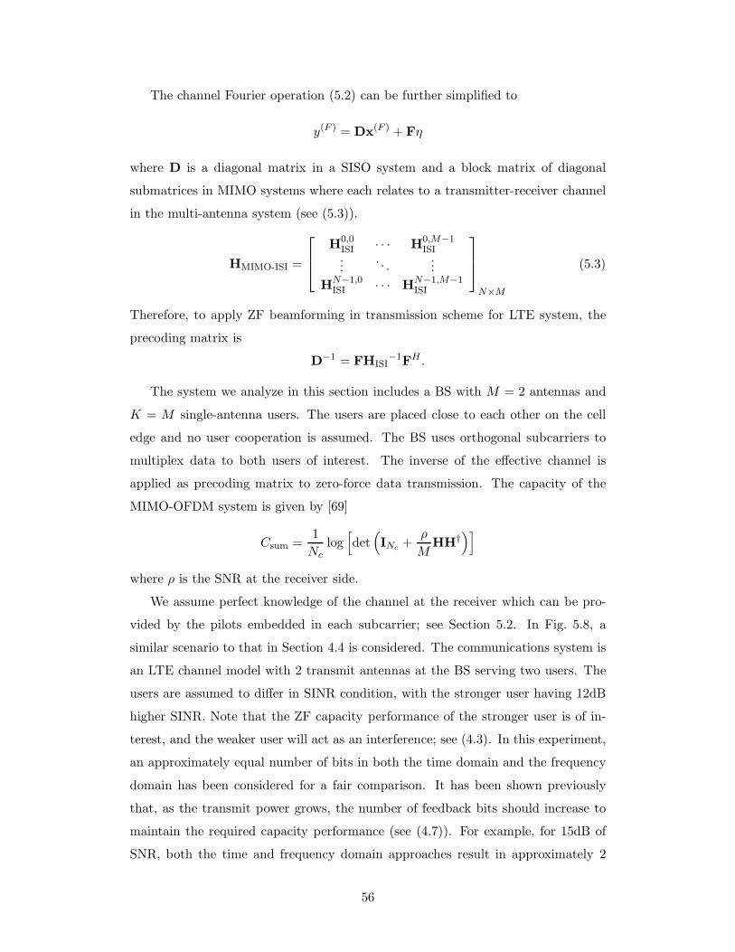
The channel Fourier operation (5.2) can be further simplified to

y(F ) = Dx(F ) + Fη

where D is a diagonal matrix in a SISO system and a block matrix of diagonal

submatrices in MIMO systems where each relates to a transmitter-receiver channel

in the multi-antenna system (see (5.3)).

HMIMO-ISI =

H0,0ISI · · · H0,M−1

ISI...

. . ....

HN−1,0ISI · · · HN−1,M−1

ISI

N×M

(5.3)

Therefore, to apply ZF beamforming in transmission scheme for LTE system, the

precoding matrix is

D−1 = FHISI−1FH .

The system we analyze in this section includes a BS with M = 2 antennas and

K = M single-antenna users. The users are placed close to each other on the cell

edge and no user cooperation is assumed. The BS uses orthogonal subcarriers to

multiplex data to both users of interest. The inverse of the effective channel is

applied as precoding matrix to zero-force data transmission. The capacity of the

MIMO-OFDM system is given by [69]

Csum =1

Nclog[

det(

INc +ρ

MHH†

)]

where ρ is the SNR at the receiver side.

We assume perfect knowledge of the channel at the receiver which can be pro-

vided by the pilots embedded in each subcarrier; see Section 5.2. In Fig. 5.8, a

similar scenario to that in Section 4.4 is considered. The communications system is

an LTE channel model with 2 transmit antennas at the BS serving two users. The

users are assumed to differ in SINR condition, with the stronger user having 12dB

higher SINR. Note that the ZF capacity performance of the stronger user is of in-

terest, and the weaker user will act as an interference; see (4.3). In this experiment,

an approximately equal number of bits in both the time domain and the frequency

domain has been considered for a fair comparison. It has been shown previously

that, as the transmit power grows, the number of feedback bits should increase to

maintain the required capacity performance (see (4.7)). For example, for 15dB of

SNR, both the time and frequency domain approaches result in approximately 2

56

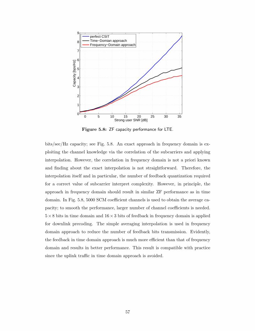
0 5 10 15 20 25 30 350

1

2

3

4

5

6

7

8

9

Strong user SNR [dB]

Cap

acity

[bps

/Hz]

perfect CSITTime−Domian approachFrequency−Domain approach

Figure 5.8: ZF capacity performance for LTE.

bits/sec/Hz capacity; see Fig. 5.8. An exact approach in frequency domain is ex-

ploiting the channel knowledge via the correlation of the subcarriers and applying

interpolation. However, the correlation in frequency domain is not a priori known

and finding about the exact interpolation is not straightforward. Therefore, the

interpolation itself and in particular, the number of feedback quantization required

for a correct value of subcarrier interpret complexity. However, in principle, the

approach in frequency domain should result in similar ZF performance as in time

domain. In Fig. 5.8, 5000 SCM coefficient channels is used to obtain the average ca-

pacity; to smooth the performance, larger number of channel coefficients is needed.

5× 8 bits in time domain and 16× 3 bits of feedback in frequency domain is applied

for downlink precoding. The simple averaging interpolation is used in frequency

domain approach to reduce the number of feedback bits transmission. Evidently,

the feedback in time domain approach is much more efficient than that of frequency

domain and results in better performance. This result is compatible with practice

since the uplink traffic in time domain approach is avoided.

57

Chapter 6

Concluding Remarks andFuture Work

The main contribution of this MSc thesis is the extension to the prior work on

feedback quantization for flat channels [32] to realistic wireless channels typical for

cellular telecommunication. Spatial Channel Model (SCM) is used to generate prac-

tical channels. In addition, we consider transmission characteristics of the practical

communications system standards, i.e., LTE. The relationship between the num-

ber of feedback bits and transmit power is analyzed for the case of different SINR

levels of the mobile users. The analytical and experimental results show that a

stronger user requires more feedback bits to maintain the same gap to capacity as

the weaker user. The second contribution is a study of feedback quantization in the

presence of imperfect CSIR. The channel is estimated at the mobile stations using

LMS algorithm. The effect of non-negligible estimation error on ZF downlink pre-

coding performance has been considered. Our results suggest that the use of larger

codebook cannot compensate for performance degradation due to estimation error.

The third contribution is a study of feedback quantization for multipath channels

and LTE downlink transmission. For the case of multipath environment, this study

shows that the time domain quantization and feedback is more practical and efficient

than frequency domain quantization and feedback. As the subcarrier correlation is

not known a priori to the feedback quantization, subcarrier interpolation results in

losses which can be avoided if quantization is performed in the time domain for each

path. Finally, the fourth contribution demonstrates that the frequency of feedback

transmission should be based on the mobility of the channel – not the frequency of

the pilot transmission. Pilot transmission is more frequent for a reliable estimation

of the channel in LTE. The frequency of feedback transmission, however, should be

58

avoided if the channel remains unchanged.

In this regard, Chapter 2 discusses the MIMO techniques for cellular networks

and interference avoidance in multiuser communications. Next, the characteristics

of the LTE system are reviewed and the Spatial Channel Model is introduced as a

realistic channel generator for this study. Chapter 3 examines the use of adaptive

filters and the family of steepest-descent algorithms. Further investigations are then

carried out by exploiting the reliability of simple and practical channel estimation

techniques - the LMS algorithm. This is to acquire channel knowledge at the receiver

with minimal error.

Chapter 4 addresses the acquiring of channel information at the transmitter.

For that purpose, the ZF capacity at the receiver is used as a metric for system

performance. Imperfect channel information is processed in terms of (a) the number

of feedback bits and the accuracy of the feedback scheme, and (b) codebook design

in more practical environments, such as different SINR situations for the users.

The consistency of the number of feedbacks, with SNR condition of the users, is

analyzed and discussed in detail. Next, the inherent complications with LTE system

are discussed in regard to the MIMO-OFDM transmission technique within the

LTE standard. The high transmission data rate and high mobility of the channel

environment in LTE system can exacerbate the degrading effect of imperfect channel

information.

Chapter 5 therefore focuses the research on this aspect and analyzes the ZF

performance in both frequency and time domain. It is shown from this analysis that

time-domain quantization feedback is far more efficient in terms of performance and

uplink overload.

Although we have studied channel estimation performance using the LMS al-

gorithm, more complex adaptive algorithms, such as RLS algorithm and Kalman

filters, are also reliable candidates for performance improvement. Channel pre-

diction due to data aging further adds new challenges to the estimation process,

especially in very mobile environments. Zero-forcing is only one of the several pre-

coding techniques for avoiding interference and maximizing throughput in receiver

antenna systems. Other precoding techniques are also of interest.

For various multipath profiles, algorithms can be designed to compress quanti-

zation feedback for error optimization. Caire et al. [70], for example, has proposed

the application of rate distortion for time-domain limited feedback. It is likely that,

59

in the near future, suboptimal quantization feedback algorithms will be a topic of

intense research interest.

Adaptive transmit antenna techniques, user selection and opportunistic signaling

will assure system capacity enhancement with the growth of the number of users

in the system. However, this requires exact knowledge of the channel. Therefore,

enriching the techniques of acquiring exact channel knowledge will enable the system

to utilize such techniques to assure capacity growth.

60

Bibliography

[1] G. T. 25.996, “Spatial channel model for multiple input multiple output(MIMO) simulations (Release 6).” 2003.

[2] A. T. Harri Holma, WCDMA For UMTS: HSPA Evolution And LTE,. NewYork: John Wiley & Sons, 2009.

[3] A. J. Paulraj, D. A. Gore, R. U. Nabar, and H. Bolcskei, “An overview ofMIMO communications - a key to gigabit wireless,” Proc. IEEE, vol. 92, pp.198–218, Feb. 2004.

[4] D. Gesbert, H. Bolcskei, D. Gore, and A. Paulraj, “MIMO wireless channels:capacity and performance prediction,” in Global Telecommunications Confer-ence, 2000. GLOBECOM ’00. IEEE, vol. 2, San Francisco, CA, Aug. 2002, pp.1083–1088.

[5] V. Tarokh, N. Seshadri, and A. R. Calderbank, “Space-time codes for high datarate wireless communication: performance criterion and code construction,”IEEE Trans. Inf. Theory, vol. 44, no. 2, pp. 744–765, Mar. 1998.

[6] S. M. Alamouti, “A simple transmit diversity technique for wireless communi-cations,” IEEE J. Sel. Areas Commun., vol. 16, no. 8, pp. 1451–1458, 1998.

[7] N. K. Das, T. Inoue, T. Taniguchi, and Y. Karasawa, “An experiment on MIMOsystem having three orthogonal polarization diversity branches in multipath-rich environment,” in Vehicular Technology Conference, 2004. VTC2004-Fall.2004 IEEE 60th, vol. 2, 2004, pp. 1528–1532.

[8] F. G. J., “Layered space-time architecture for wireless communication,,” BellLabs Technical Journal, vol. 1, pp. 41–59, 1996.

[9] A. J. Paulraj and T. Kaillath, “Increasing capacity in wireless broadcast sys-tems using distributed transmission/directional reception,,” Bell Labs TechnicalJournal, 1994.

[10] C. E. Shannon, “The mathematical theory of communication,,” Bell Syst, TechJ., vol. 27, no. 2, pp. 379–423, 1948.

[11] C. C. Martin, J. H. Winters, and N. R. Sollenberger, “Multiple-input multiple-output (MIMO) radio channel measurements,” in Antennas and PropagationSociety International Symposium, 2001. IEEE, vol. 1, Boston, MA, Jul. 2001,pp. 418–421.

[12] J. Ling, D. Chizhik, P. Wolniansky, R. Valenzuela, N. Costa, and K. Huber,“Multiple transmit multiple receive (MTMR) capacity survey in manhattan,”Electronics Letters, vol. 37, no. 16, pp. 1041–1042, Aug. 2001.

[13] R. M. Buehrer, S. Arunachalam, K. H. Wu, and A. Tonello, “Spatial chan-nel model and measurements for IMT-2000 systems,” in Vehicular TechnologyConference, 2001. VTC 2001 Spring. IEEE VTS 53rd, vol. 1, Rhodes, May2001, pp. 342–346.

61

[14] D. Astely, E. Dahlman, A. Furuskar, Y. Jading, M. Lindstrom, and S. Parkvall,“LTE: the evolution of mobile broadband,” IEEE Commun. Mag., vol. 47, pp.44–51, Apr. 2009.

[15] P. V. David Tse, Fundamentals of Wireless Communications,. New York:Cambridge Press University, 2005.

[16] G. J. Foschini and M. J. Gans, “On limits of wireless communications in afading environment when using multiple antennas,” Wirel. Pers. Commun.,vol. 6, no. 3, pp. 311–335, 1998.

[17] E. Telatar, “Capacity of multi-antenna Gaussian channels,” European Trans-actions on Telecommunications, vol. 10, no. 6, pp. 585–596, 1999.

[18] S. Maruyama, S. Ogawa, and K. Chiba, “Mobile terminals toward LTE andrequirements on device technologies,” in VLSI Circuits, 2007 IEEE Symposiumon, Kyoto, Jun. 2007, pp. 2–5.

[19] Zyren, “Overview of the 3gpp long term evolution physical layer,,” Dr. WesMcCoy, Tech. Rep., 2007.

[20] E. Damosso and L. M. Carreia, “Cost 231 final report,”http://www.gsmworld.com/, 1999.

[21] S. Haykin, Adaptive Filter Theory, 2nd ed. Prentice Hall, 1991.

[22] H. Zhu, B. Farhang-Boroujeny, and C. Schlegel, “Pilot embedding for jointchannel estimation and data detection in MIMO communication systems,”IEEE Commun. Lett., vol. 7, pp. 30–32, Jan. 2003.

[23] B. Farhang-Boroujeny, “Pilot-based channel identification: proposal for semi-blind identification of communication channels,” Electronics Letters, vol. 31,pp. 1044–1046, Jun. 1995.

[24] C. K. Ho, B. Farhang-Boroujeny, and F. Chin, “Added pilot semi-blind channelestimation scheme for OFDM in fading channels,” in Global Telecommunica-tions Conference, 2001. GLOBECOM ’01. IEEE, vol. 5, San Antonio, TX, Nov.2001, pp. 3075–3079.

[25] J. K. Cavers, “An analysis of pilot symbol assisted 16QAM for digital mobilecommunications,” in Vehicular Technology Conference, 1991. Gateway to theFuture Technology in Motion., 41st IEEE, St. Louis, MO , USA, Nov. 1991,pp. 380–385.

[26] C. E. Shannon, “The zero error capacity of a noisy channel,” IRE Trans. In-form. Theory, Sep. 1956.

[27] F. Floren, O. Edfors, and B. A. Molin, “The effect of feedback quantization onthe throughput of a multiuser diversity scheme,” in Global TelecommunicationsConference, 2003. GLOBECOM ’03. IEEE, vol. 1, Dec. 2003, pp. 497–501.

[28] T. Tang and R. W. Heath, “Opportunistic feedback for downlink multiuserdiversity,” IEEE Commun. Lett., vol. 9, no. 10, pp. 948–950, Oct. 2005.

[29] P. Viswanath, D. N. C. Tse, and R. Laroia, “Opportunistic beamforming us-ing dumb antennas,” in Information Theory, 2002. Proceedings. 2002 IEEEInternational Symposium on, Jun. 2002.

[30] T. Yoo, N. Jindal, and A. Goldsmith, “Multi-antenna downlink channels withlimited feedback and user selection,” IEEE J. Sel. Areas Commun., vol. 25,no. 7, pp. 1478–1491, Sep. 2007.

62

[31] N. Chiurtu, B. Rimoldi, and E. Telatar, “On the capacity of multi-antennagaussian channels,” in Information Theory, 2001. Proceedings. 2001 IEEE In-ternational Symposium on, Washington, DC, Jun. 2001.

[32] N. Jindal, “MIMO broadcast channels with finite-rate feedback,” IEEE Trans.Inf. Theory, vol. 52, no. 11, pp. 5045–5060, Nov. 2006.

[33] D. J. Love, J. Heath, R. W., W. Santipach, and M. L. Honig, “What is thevalue of limited feedback for MIMO channels?” IEEE Commun. Mag., vol. 42,no. 10, pp. 54–59, Oct. 2004.

[34] D. J. Love, R. W. Heath, V. K. N. Lau, D. Gesbert, B. D. Rao, and M. Andrews,“An overview of limited feedback in wireless communication systems,” IEEEJ. Sel. Areas Commun., vol. 26, no. 8, pp. 1341–1365, Oct. 2008.

[35] D. J. Love, J. Heath, R. W., and T. Strohmer, “Grassmannian beamformingfor multiple-input multiple-output wireless systems,” IEEE Trans. Inf. Theory,vol. 49, no. 10, pp. 2735–2747, Oct. 2003.

[36] C. Simon and G. Leus, “Feedback quantization for linear precoded spatial mul-tiplexing,” EURASIP J. Adv. Signal Process, vol. 2008, pp. 1–13, 2008.

[37] W. Santipach, “Tree-structured random vector quantization for beamformingin a multiantenna channel,” in Electrical Engineering/Electronics, Computer,Telecommunications and Information Technology, 2008. ECTI-CON 2008. 5thInternational Conference on, vol. 1, Krabi, 2008, pp. 325–328.

[38] R. Samanta and R. W. Heath, “Codebook adaptation for quantized MIMObeamforming systems,” in Signals, Systems and Computers, 2005. ConferenceRecord of the Thirty-Ninth Asilomar Conference on, Pacific Grove, CA, Oct.2005, pp. 376–380.

[39] V. Raghavan, R. W. Heath, and A. V. Sayeed M., “Systematic codebook designsfor quantized beamforming in correlated MIMO channels,” IEEE J. Sel. AreasCommun., vol. 25, no. 7, pp. 1298–1310, Sep. 2007.

[40] A. Gersho and R. M. Gray, Vector Quantization and Signal Compression.Boston: Kluwer,, 1992.

[41] Y. Linde, A. Buzo, and R. Gray, “An algorithm for vector quantizer design,”IEEE Trans. Commun., vol. 28, no. 1, pp. 84–95, Jan. 1980.

[42] A. Narula, M. J. Lopez, M. D. Trott, and G. W. Wornell, “Efficient use of sideinformation in multiple-antenna data transmission over fading channels,” IEEEJ. Sel. Areas Commun., vol. 16, no. 8, pp. 1423–1436, Oct. 1998.

[43] J. H. Conway, R. H. Hardin, and N. J. A. Sloane, “Packing lines, planes, etc.:Packings in grassmannian spaces,” Exper. Math., vol. 5, no. 2, pp. 139–159,1996.

[44] N. J. A. Sloane, “Packings in grassmannian spaces,”http://www.research.att.com/∼njas/grass/.

[45] G. Caire, N. Jindal, M. Kobayashi, and N. Ravindran, “Multiuser MIMOachievable rates with downlink training and channel state feedback,” IEEETrans. Inf. Theory, vol. 56, no. 6, pp. 2845–2866, May 2009.

[46] A. Bahai and B. Saltzberg, Multi-Carrier Digital Communications, Theory andApplication of OFDM. Kluwer Academics, 2002.

[47] S. H. Han and J. H. Lee, “An overview of peak-to-average power ratio reduc-tion techniques for multicarrier transmission,” IEEE Trans. Wireless Commun.,vol. 12, pp. 56–65, Apr. 2005.

63

[48] S. Kasturia and J. M. Aslanis, J. T. Cioffi, “Vector coding for partial responsechannels,” IEEE Trans. Inf. Theory, vol. 36, pp. 741–762, Jul. 1990.

[49] J. M. Cioffi, “Digital communications, chapter 4: Multichannel modulation,”Unpublished course notes.

[50] A. Goldsmith, Wireless Communications. New York: Cambridge Press Uni-versity, 2005.

[51] 3rd Generation Partnership Project, “Technical specification group radio accessnetwroks; deployment aspects,,” Tech. Rep. 7, June 2007.

[52] L. A. M. Ruiz de Temino, C. Navarro i Manchon, C. Rom, T. B. Sorensen, andP. Mogensen, “Iterative channel estimation with robust wiener filtering in LTEdownlink,” in Vehicular Technology Conference, 2008. VTC 2008-Fall. IEEE68th, Calgary, BC, 2008, pp. 1–5.

[53] Y. Zhao and A. Huang, “A novel channel estimation method for OFDM mobilecommunication systems based on pilot signals and transform-domain process-ing,” in Vehicular Technology Conference, 1997 IEEE 47th, vol. 3, Phoenix,AZ, 1997, pp. 2089–2093.

[54] M.-H. Hsieh and C.-H. Wei, “Channel estimation for OFDM systems basedon comb-type pilot arrangement in frequency selective fading channels,” IEEETrans. Consum. Electron., vol. 44, no. 1, pp. 217–225, Feb. 1998.

[55] A. K. Jagannatham and B. D. Rao, “Whitening-rotation-based semi-blindMIMO channel estimation,” IEEE Trans. Signal Process., vol. 54, no. 3, pp.861–869, Mar. 2006.

[56] N. Michelusi, “Semi-blind channel estimation for lte downlink,” Master’s thesis,Thechnical University of Denmark, jun 2009.

[57] M. M. Rana, J. Kim, and W.-K. Cho, “Low complexity downlink channel esti-mation for LTE systems,” in Advanced Communication Technology (ICACT),2010 The 12th International Conference on, vol. 2, Phoenix Park, 2010, pp.1198–1202.

[58] B. Karakaya, H. Arslan, and H. A. Curpan, “Channel estimation for LTE up-link in high Doppler spread,” in Wireless Communications and NetworkingConference, 2008. WCNC 2008. IEEE, Las Vegas, NV, 2008, pp. 1126–1130.

[59] A. Ancora, C. Bona, and D. T. M. Slock, “Down-sampled impulse responseleast-squares channel estimation for LTE OFDMA,” in Acoustics, Speech andSignal Processing, 2007. ICASSP 2007. IEEE International Conference on,vol. 3, Honolulu, HI, 2007, pp. 293–296.

[60] B. Hassibi, A. H. Sayed, and T. Kailath, “H optimality of the lms algorithm,”IEEE Trans. Signal Process., vol. 4, no. 2, pp. 267–280, Aug. 1995.

[61] J. Berkmann, C. Carbonelli, F. Dietrich, C. Drewes, and W. Xu, “On 3GLTE terminal implementation - standard, algorithms, complexities and chal-lenges,” in Wireless Communications and Mobile Computing Conference, 2008.IWCMC ’08. International, Crete Island, 2008, pp. 970–975.

[62] “Requirements for eutra and eutran,,” 3GPP, Tech. Rep., 2006.

[63] J. G. Proakis, Digital Communications. McGraw-Hill, 2001.

[64] M. K. Ozdemir and H. Arslan, “Channel estimation for wireless OFDM sys-tems,” IEEE Commun. Surveys Tuts., vol. 9, no. 2, pp. 18–31, 2007.

64

[65] Z. Jianhua and Z. Ping, “An improved 2-dimensional pilot-symbols assistedchannel estimation in OFDM systems,” in Vehicular Technology Conference,2003. VTC 2003-Spring. The 57th IEEE Semiannual, vol. 3, Jul. 2003, pp.1595–1599.

[66] A. Dowler, A. Doufexi, and A. Nix, “Performance evaluation of channel esti-mation techniques for a mobile fourth generation wide area OFDM system,”in Vehicular Technology Conference, 2002. Proceedings. VTC 2002-Fall. 2002IEEE 56th, vol. 4, Dec. 2002, pp. 2036–2040.

[67] R. W. S. Alan V. Oppenheim, Discrete-Time Signal Processing,. New Jersey:Prentice-Hall Inc., 1999.

[68] J. Wang, S. Zhu, and L. Wang, “On the channel capacity of MIMO-OFDMsystems,” in Communications and Information Technology, 2005. ISCIT 2005.IEEE International Symposium on, 2005, pp. 1372–1375.

[69] H. Bolcskei, D. Gesbert, and A. J. Paulraj, “On the capacity of OFDM-basedspatial multiplexing systems,” IEEE Trans. Commun., vol. 50, no. 2, pp. 225–234, Feb. 2002.

[70] G. Caire and H. Shirani-Mehr, “Feedback schemes for multiuser MIMO-OFDMdownlink,” in Information Theory and Applications Workshop, San Diego, CA,2008, pp. 33–40.

65