Inequality, Opting-out and Public EducationFunding

Calin Arcalean∗

ESADE

Ioana Schiopu†

ESADE and CESifo

June 2015

Abstract

We investigate the effect of inequality on the political support for public edu-cation funding in a model of endogenous fertility and school choice. In contrast torecent literature we show that when household income heterogeneity is consistentwith the skewness of empirical income distributions, inequality can drive educa-tion spending in opposite directions in poor and rich economies. A mean preserv-ing spread increases tax rates and public school enrollment, but decreases publicspending per student in low income economies, while it has opposite effects at highincome levels. An increase in the average income level can also have non-monotoniceffects.

JEL Codes: D72, H42, I21, I22.Keywords: Education funding, Inequality, Political Economy.

∗The authors gratefully acknowledge financial support from Generalitat de Catalunya (grant SGR

2014-1079) and Banc Sabadell.†Corresponding author. Email: ioana.schiopu@esade.edu, ESADE Business School, Ramon Llull

University, Avenida de Torreblanca 59, 08172 Sant Cugat del Vallès, Barcelona, Spain, phone: +34 934

952 327.

1

1 Introduction

Public provision of basic education is a major form of redistribution virtually every-

where. As income inequality is on the rise in most countries, investigating the repercus-

sions for public education funding becomes a relevant issue given the particular role of

human capital differences in perpetuating economic and social disparities. So far how-

ever, empirical work on the link between redistribution and inequality has generated,

across a variety of time periods and datasets, rather inconclusive results indicating a

more complex, potentially nonlinear relation.1 For example, a look at public education

funding across U.S. states reinforces this view. Figure 1 suggests the relationship between

inequality and per pupil state revenues, conditional on a set of standard controls, may

change depending on the level of per capita income. These findings seem to warrant fur-

ther theoretical efforts aimed at better understanding specific redistribution mechanisms.

Figure 1: Public education revenues per pupil and inequality

-.01

0.0

1.0

2.0

3.0

4

.3 .35 .4 .45Lagged Gini

(a)

-.02

-.01

0.0

1.0

2.0

3

.34 .36 .38 .4 .42 .44Lagged Gini

(b)

Notes: The analysis uses decadal U.S. state-level panel data, 1970-2000. The dependent variableis per pupil state revenues, expressed as a share of state income per capita. The semiparametricfixed effects estimator of Baltagi and Li (2002) is used to partial out control variables includinga full set of fixed effects. Panels (a) and (b) depict the nonparametric relation between theresulting error component and the 10 year lagged Gini index, for states with per capita laggedincome below and respectively above an income threshold set equal to 1.09 of the sample medianvalue. Results are robust to alternative income thresholds. Shaded bands are 95 percentconfidence intervals based on robust, state level clustered, standard errors. See Appendix Cfor details on the estimation, variable definitions and data sources.

In this paper we study a political economy model of public education provision with

a private schooling option and endogenous fertility decisions. Importantly, we allow

household income heterogeneity to be consistent with the skewness of empirical income1A number of papers have found that support for redistribution is weaker in more unequal or more

heterogenous societies (Goldin and Katz (1997), Alesina et al. (1999, 2001), Lindert (1996), Luttmer(2001)). Perotti (1996) finds no relationship between inequality and redistribution in democracies. Morerecently, Boustan et al. (2010) find that rising inequality is associated with higher local revenue collectionand expenditures.

2

distributions, where the median is lower than the mean income. Tax financed uniform

public education quality is insuffi cient for rich parents who choose to send their children

to a private school.2 This generates an endogenous income threshold that separates public

and private school users. Ceteris paribus, the higher the public school quality, the lower

the private enrollment share. Reflecting a quantity-quality trade-off, households opting

for private education choose a lower fertility rate than those opting for public schooling.

For transparency, fertility is constant within groups.

The equilibrium public spending arises as the politically mediated balance between

the conflicting interests of public and private school users. On the one hand, those opting

for private schooling want to minimize the tax burden. On the other hand, those who

choose public schooling, want to ensure adequate spending per student. In this setting

we study how the political balance and thus the equilibrium education spending and

enrollment respond in two counterfactual experiments: a) a mean preserving spread of

the income distribution and b) an increase in the tax base keeping income dispersion

constant.

First, we show that inequality can drive education spending in opposite directions in

poor and rich economies. A mean preserving spread increases tax rates (spending per

capita) and public school enrollment, but decreases public spending per student in low

income economies, while it has opposite effects at high income levels. A marginal increase

in the tax base, holding income dispersion constant, can also have non-monotonic effects.

Furthermore, tax base and inequality effects on redistribution depend critically on the

parental preferences for quality versus quantity of children.

When inequality increases, the tails of the income distribution (the poor and rich

groups) get larger, while the middle income group shrinks. In a poor economy where

fertility rates are high and/or the tax base is low, public schools are of low quality, so a

large share of the middle income households use private schools (the endogenous income

threshold is far from the right tail). A mean preserving spread produces a replacement

of these families by high fertility low income families that choose public education. This

shift in school choice dominates the negative effect on redistribution generated by a larger

rich group. Consequently, the interests of the poor dominate and thus the support for

public education increases. However, the endogenous enrollment in public school rises at

a faster rate than resources, depressing spending per student. In contrast, when the tax

base is high, as in a rich economy, most households from the middle group use public

education (the indifference income threshold is close to the right tail). The replacement

of families from the middle group by poor ones does not produce a large positive effect

on the support for redistribution as the two groups have the same school choice. Thus

2The 2011/7 OECD report ‘PISA in Focus’states that in the 26 economies surveyed, "the typicalstudent enrolled in private schools outperforms the typical public school student" with the "private schooladvantage" being "equivalent to three-quarters of a year’s worth of formal schooling."

3

the larger rich income group steers the political process in their favor, lowering the tax

rate and spending on public education. However, the overall public spending per student

increases as resources decrease at a lower rate than the endogenous enrollment.

As a benchmark, we focus on probabilistic voting with households that have uniform

political power. Asymmetric distribution of political power is typically associated with

authoritarian regimes or partially democratic countries. However, it can also arise in well

established democracies if, as documented by the literature on political participation,

voter turnout varies systematically with demographic characteristics. We extend the

model to include an income based index of political power and study its properties. The

effects on per student spending and enrollment in public schools are preserved under

an empirically relevant degree of political power. In contrast to the benchmark model

however, the tax rate can decrease even in the poor economies when inequality increases,

depressing the public spending per student even further.

Our results are significant in at least three dimensions. First, we conceptually de-

compose inequality variation into a tax base change and a pure income dispersion effect

and explain the non-trivial role each component plays in determining public spending

for education and enrollment in public schools. Second, the theoretical analysis helps

illuminate empirical work. On the one hand, the non-monotonic response of redistribu-

tion in our framework may justify some of the conflicting results obtained so far in the

literature. On the other hand, and more importantly, we provide an alternative frame-

work to think about differences in redistribution through public education. For example,

while typical regressions include the median income, our theory suggests controlling for

the mean income both directly and through its interactions with dispersion measures.

Finally, our results imply a novel mechanism of inequality amplification arising through

the endogenous determination of public education spending. To the extent spending per

student is important for human capital formation, and thus, future income, diverging

public education funding at different mean income levels can widen the initial income

disparities.

1.1 Connections to the literature

Our paper contributes to the theoretical literature studying the effects of inequality on

public goods provision and income redistribution. While some political economy papers

argue that higher inequality leads to more redistribution through higher taxation (Meltzer

and Richard (1981), Persson and Tabellini (1994), Bénabou (1997)), others find that

more unequal or more heterogenous societies spend less on public goods (Soares (1998),

de la Croix and Doepke (2009)). Glomm (2004) finds that the relationship between

inequality and the amount of redistribution through public education services depends

on the elasticity of substitution between consumption and the quality of education in

4

the parent’s utility. He finds that for empirically relevant value of this parameter, higher

inequality generates less redistribution.

Bénabou (1997, 2000) and Lee and Roemer (1998) focus on capital market imperfec-

tions to show that non-monotonic responses of redistribution to inequality are possible.

Fernandez and Levy (2008) also find a non-monotonic effect of increased diversity in a

model with income and preference heterogeneity. Complementary to these studies, we

obtain a non-monotonic effect of inequality on redistribution at different levels of the av-

erage income per capita stemming from endogenous fertility and education choices. Also,

in these papers, redistribution occurs through progressive taxation (Bénabou (2000)) or

the provision of universal public education (Lee and Roemer (1998)). In the latter case,

private and public investments in education are complements, but only the rich house-

holds top up. In contrast, we focus on public education funding when the rich can opt

out of the public system.

While the paper builds on de la Croix and Doepke (2009), our analysis focuses on the

effects of inequality on redistribution rather than on the nature of the implemented edu-

cation system (segregation vs integration). Using a uniform distribution and a normalized

mean income (tax base), they obtain a positive relationship between higher inequality

and public spending per pupil. Our framework is different in three important ways.

First, we allow for changes in the mean income who in turn affect the size of the tax

base. This allows us to study the effects of exogenous changes in the mean income of

the economy. Second, we build our analysis on empirically relevant income distributions

(rightly skewed). The implicit asymmetry in the mass of rich and poor households gener-

ates equilibrium schooling and aggregate fertility outcomes that depend on both income

dispersion and the mean income. In contrast with previous literature, in our model the

effects of higher income dispersion on spending and enrollment in public schools are non-

monotonic in the mean income of the economy. Thus, we recover the result from de la

Croix and Doepke (2009) as a particular case and show that inequality can generate a

lower public spending per pupil for economies with lower mean income or higher fertility

preferences. Finally, we introduce a parsimonious and tractable index of political power

that derives naturally from the underlying income distribution and has a straightforward

data counterpart. In our framework a unique equilibrium always exists for empirically

relevant values of the political power parameter.

In contrast to models that study how sorting across communities affects public goods

provision and inequality3, in this paper we study how education funding responds to

exogenous changes in inequality, driven by national or global factors (e.g. skill biased

technological change, international trade) rather then by sorting incentives. Recent em-

pirical studies (e.g. Cutler et al. (1999), Rhode and Strumpf (2003) and Baicker et al.

3See, for example, Epple et al. (1993), Epple and Platt (1998), Bénabou (1994), Bénabou (1996),Fernandez and Rogerson (1996), Bearse et al. (2001).

5

(2012)) have shown that even in the United States, the textbook example of Tiebout

sorting, segregation across communities has been constant or even declined, suggesting

that the rise in income inequality across school districts, metropolitan statistical areas or

states in recent decades cannot be explained by Tiebout sorting alone.

The remainder of the paper is structured as follows. Section 2 presents the model.

Section 3 defines the equilibrium and derives the main analytical results. Section 4

documents significant participation differences in local politics related to public education

provision and extends the benchmark model by incorporating political power. Section

5 concludes. Proofs are relegated to Appendix A. Appendix B is devoted to robustness

analysis.

2 The model

2.1 The Economy

The economy is populated by a large number of households, which are heterogenous

in income. The mass of households is normalized to one. Each household consists of an

adult and a number of children. Children are educated either in public schools, which

are financed by a consumption tax, or in private schools, financed by parental spending.

Household income is distributed according to a Pareto distribution, with p.d.f. f and

c.d.f. F , with parameters xl > 0 and α > 2, and support x ∈ [xl;∞) .4 The Pareto

distribution is used for tractability reasons (see also Lee and Roemer (1998)). Other

distributions used in the literature yield similar qualitative results. As a robustness

check, in Section 1 of Appendix B we replicate the main results numerically using a

log-normal income distribution.

The mean and standard deviation of the income distribution are given by:

µ =α

α− 1xl and σ =

xlα− 1

√α

α− 2. (1)

Adults derive utility from net of tax consumption c, the number of children n and

the quality of their education h, which can be private or public. Private education has a

unit price. Let s denote the quality of public schools. Households can opt out of publicly

provided education and send their children to a private school of quality er. Following

de la Croix and Doepke (2009), the preferences are given by:

u(c, n, h) = ln(c) + γ [ln(n) + η ln(h)] , (2)

where h = s, er, γ > 0 and η ∈ (0, 1).4The p.d.f. is given by f(x) = αxαl /x

α+1, for y > yl and zero otherwise. The c.d.f. is F (x) =1− (xl/x)α .

6

The assumption of logarithmic utility is consistent with the empirical evidence, which

suggests that income and substitution elasticities of education spending have similar

magnitudes (see Gradstein et al. (2005), pg. 50-51 for a discussion).

The government taxes the consumption of all households at the constant rate τ . Tax

revenues are used to finance public education of uniform quality given by spending per

student.

The public policy is determined through a probabilistic voting mechanism described

below. Private choices on fertility and education are made before voting on the quality

of public education takes place. Agents have perfect foresight regarding the outcome of

the voting process. Thus, in equilibrium, the expected spending per student in public

education equals the level chosen by voting.

This timing reflects the sizeable differences in the relative costs and time horizons

of the decisions involved. While public education spending is usually decided through

yearly budget votes, fertility and child rearing decisions cannot be easily adjusted at

this frequency and depend largely on "pre-determined" characteristics, such as income,

education level, race, religion, etc. A similar argument applies to the choice between

public and private schooling, which in general are tightly connected to residential choice

and therefore can entail substantial switching costs.5

Furthermore, under perfect foresight, a quantity-quality trade-off maps fertility de-

cisions into consistent school choices. Therefore, even if households decide on private

vs. public education after policies are set, as long as fertility decisions occur before the

vote on public education quality, the same equilibrium will obtain as under the original

timing.6

2.2 Household’s problem

Rearing children involves a time cost. Denote by φ ∈ (0, 1) the fraction of the parent’s

time spent raising a child, and with Up and U r the utility of households whose children

are educated in the public and private schools, respectively. Given the expected quality

of publicly provided education E[s] and the tax rate τ , a household with income x that

chooses public education solves the following problem:

max{c≥0,n≥0}

Up(c, n, E[s]) = ln(c) + γ ln(n) + γη ln(E[s]), (3)

s.t. c(1 + τ) ≤ x(1− φn). (4)

The solution of problem (3) is np = γ/ [φ(1 + γ)] .

5de la Croix and Doepke (2009) also conclude that in countries where the educational and residentialsegregation are correlated, private decisions generate strong lock-in effects.

6See Dottori and Shen (2009) for a related discussion.

7

On the other hand, a household choosing private education solves:

max{c≥0,n≥0,er≥0}

U r(c, n, er) = ln(c) + γ ln(n) + γη ln(er), (5)

s.t. c(1 + τ) + ner ≤ x(1− φn). (6)

The solutions to the problem (5) are nr = [γ(1− η)] / [φ(1 + γ)] and er = φηx/(1−η).7

Comparing np and nr we see that while fertility rates are constant within each group,

households that choose private schooling have a lower fertility than those sending their

children to public schools. Consumption of both household types is a constant share of

income c = x/((1 + γ)(1 + τ)).8

Substituting np in (3) and nr and er in (5) we obtain the indirect utilities of households

that choose public and private schooling, respectively:

V p(x, s, τ) = ln

[x

(1 + γ) (1 + τ)

]+ γ ln

[γ

φ(1 + γ)

]+ γη ln(E[s]) (7)

and

V r(x, τ) = ln

[x

(1 + γ) (1 + τ)

]+ γ ln

[γ(1− η)

φ(1 + γ)

]+ γη ln

[φηx

1− η

]. (8)

A household will choose public education if and only if V p(x, s, τ) ≥ V r(x, τ). This

inequality is satisfied for households with income lower than a threshold x, given by:

x =(1− η)E[s]

δφη, where δ = (1− η)

1η ∈ (0, 1), (9)

where E[s] represents the expected quality of education.

Households choose the school type taking the other households’decisions as given.

Denote by Ψ the fraction of households that choose public schooling:

Ψ = F (x) =

∫ x

xl

f(x)dx = 1−(xlx

)α. (10)

The fraction of children in public schools is then given by:

N =npΨ

npΨ + nr(1−Ψ). (11)

7The constant fertility and share of education spending in total income are due to homothetic pref-erences over the bundle (c, n, h). However, numerical simulations show results are preserved in a frame-work with non-homothetic preferences as long as the share of private education spending is increasingin income. Thus the fertility differential between the rich and poor households increases with income.Consider the following example: u(c, n, h) = ln(c) + γ [ln(n) + η ln(h+ κ)] , where κ > 0. This yieldser/y = (yηφ − κ)/((1 − η)y), with ∂(er/y)/∂y > 0, and nr = γy(1 − η)/((1 + γ)(yφ − κ)), where∂nr/∂y < 0.

8de la Croix and Doepke (2009) obtain similar results assuming an income tax and tax deductibilityof private education spending.

8

Substituting the expressions for np and nr we obtain:

N =Ψ

(1− η) + ηΨ> Ψ. (12)

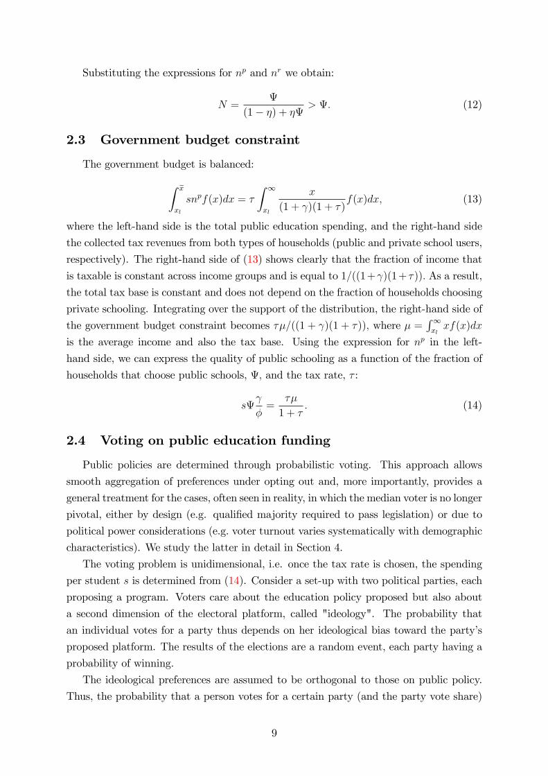
2.3 Government budget constraint

The government budget is balanced:∫ x

xl

snpf(x)dx = τ

∫ ∞xl

x

(1 + γ)(1 + τ)f(x)dx, (13)

where the left-hand side is the total public education spending, and the right-hand side

the collected tax revenues from both types of households (public and private school users,

respectively). The right-hand side of (13) shows clearly that the fraction of income that

is taxable is constant across income groups and is equal to 1/((1+γ)(1+ τ)). As a result,

the total tax base is constant and does not depend on the fraction of households choosing

private schooling. Integrating over the support of the distribution, the right-hand side of

the government budget constraint becomes τµ/((1 + γ)(1 + τ)), where µ =∫∞xlxf(x)dx

is the average income and also the tax base. Using the expression for np in the left-

hand side, we can express the quality of public schooling as a function of the fraction of

households that choose public schools, Ψ, and the tax rate, τ :

sΨγ

φ=

τµ

1 + τ. (14)

2.4 Voting on public education funding

Public policies are determined through probabilistic voting. This approach allows

smooth aggregation of preferences under opting out and, more importantly, provides a

general treatment for the cases, often seen in reality, in which the median voter is no longer

pivotal, either by design (e.g. qualified majority required to pass legislation) or due to

political power considerations (e.g. voter turnout varies systematically with demographic

characteristics). We study the latter in detail in Section 4.

The voting problem is unidimensional, i.e. once the tax rate is chosen, the spending

per student s is determined from (14). Consider a set-up with two political parties, each

proposing a program. Voters care about the education policy proposed but also about

a second dimension of the electoral platform, called "ideology". The probability that

an individual votes for a party thus depends on her ideological bias toward the party’s

proposed platform. The results of the elections are a random event, each party having a

probability of winning.

The ideological preferences are assumed to be orthogonal to those on public policy.

Thus, the probability that a person votes for a certain party (and the party vote share)

9

is a smooth function of the distance between the two platforms. This framework has a

unique equilibrium in which both parties converge to the same platform (see Persson and

Tabellini (2002)), which maximizes the following social welfare function:

W (τ) =

∫ x

xl

V P (x, np, s, τ)p(x)f(x)dx+

∫ ∞x

V R(x, nr, er, τ)p(x)f(x)dx, (15)

subject to the government budget constraint (14).

The first (second) term of the welfare function is the aggregate utility of the households

that choose public (private) education, respectively. The term p(x) captures the political

power of the group. We first assume p(x) = 1, that is, all voters have the same political

power. We relax this assumption in Section 4.

Since fertility and education choices are determined before the vote takes place, the

income threshold x is taken as given in the maximization of 15.

Substituting the indirect utility functions, (7) and (8), in (15) and grouping terms,

we get:

W (τ) = ln

(1

(1 + γ)(1 + τ)

)+ γ ln

[γ

φ(1 + γ)

]+ γη ln(s(τ))

∫ x

xl

f(x)dx+∫ ∞x

{γ ln(1− η) + γη ln

[φηx

1− η

]}f(x)dx.

Since only the first and the third term are functions of the policy variables, the welfare

can be rewritten (with abuse of notation) as

W (τ) = − ln(1 + τ) + γηΨ ln(s(τ)), (16)

where Ψ(x) is taken as given. Substituting s from (14) and taking the first order condition

with respect to τ yields:

τ = γηΨ. (17)

Everything else equal, the tax increases with the households’concern for children as

well as with the fraction of households using public education. In the next section we

define the equilibrium and study its properties.

3 Equilibrium analysis

Definition 1. A politico-economic equilibrium is an income threshold x satisfying (9),

private allocations (cp, np) if x ≤ x, (cr, nr, er) if x > x, and a public policy (s, τ) such

that:

10

(i) household’s decisions solve problems (3) or (5), given expected public education

quality E[s];

(ii) the government budget is balanced, i.e. it satisfies (14);

(iii) the tax rate τ solves the social welfare maximization problem (15);

(iv) households have perfect foresight: s = E[s].

Next, we solve for the equilibrium threshold x. To minimize clutter, we drop functional

dependencies where possible. We use the expression of s, (14), and τ , (17) in (9) to obtain:

x =µ

δ

1− η1 + γηΨ(x)

. (18)

Using (10) yields the following equation:

x =µ

δ

1− η1 + γη

[1−

(xlx

)α] . (19)

Equation (19) shows that in equilibrium, households’private education decisions are

consistent with the aggregate outcomes.

Proposition 1. There exists a unique and interior equilibrium income threshold x∗ ∈(xl,∞) that solves equation (19) (proof in the Appendix).

Note that the equilibrium threshold x∗ is always interior because the support of the

income distribution does not have an upper bound. When x∗ → ∞, the fraction ofstudents in public schools goes asymptotically to 1. Equilibrium uniqueness also owes

to the endogenous fertility, which ensures that the tax base is independent of public

education enrollment and thus the right hand side of equation (19) is decreasing in Ψ.

Proposition 1 implies there is a unique equilibrium public spending per student:

s∗ =x∗φηδ

1− η =φηµ

1 + γη[1−

( xlx∗

)α] . (20)

We use equations (10) and (20) to express Ψ∗ as a function of s∗:

Ψ∗ =1

γη

(φηµ

s∗− 1

). (21)

Using (10) in (12), we obtain the equilibrium enrollment in public schools:

N∗ =Ψ∗

(1− η) + ηΨ∗, where Ψ∗ = 1−

( xlx∗

)α. (22)

In the following, we investigate how changes in the income distribution affect the main

policy variables. We focus on two experiments: a) a change in the average income per

11

capita µ, keeping the standard deviation σ constant and b) a mean preserving spread in

the income distribution (change σ while keeping µ constant).

3.1 A change in the mean income (tax base)

Now we analyze the effects of changing the mean income, µ, on the equilibrium public

spending per student s∗, the tax rate τ ∗, and enrollment in public schools N∗. Recall

that in our model µ also represents the tax base.

Denote by d(µ, σ) = [xl(µ, σ)/x(µ, σ)]α(µ,σ). The derivative of N∗ with respect to µ is:

∂N∗

∂µ=

1− η[(1− η) + ηΨ∗]2

∂Ψ∗

∂µ(23)

=1− η

[(1− η) + ηΨ∗]2φ

γ

s∗ − µ∂s∗∂µ

(s∗)2,

where

∂s∗

∂µ=

φη

{1 + γη(1− d) + µγη

∂d(µ, σ)

∂µ

}[1 + γη(1− d)]2

. (24)

Using (17) and (21) we obtain the change in the equilibrium tax rate with respect to

µ:∂τ ∗

∂µ= γη

∂Ψ∗

∂µ.

Thus, sign(∂τ ∗/∂µ) = sign(∂Ψ∗/∂µ) = sign(∂N∗/∂µ). Studying the properties of

the function ∂N∗/∂µ yields the following results.

Proposition 2. Let γ = {[2(1 − η)/(δe)] − 1}/ {η [1− e−2]} and γ = {[(1 − η)/δ] −1}/ {η [1− (1/e)]} , where e is the Euler’s constant.1) If γ 6 γ, then ∂N∗/∂µ > 0 and ∂τ ∗/∂µ > 0;

2) If γ > γ, then ∂N∗/∂µ < 0 and ∂τ ∗/∂µ < 0;

3) If γ ∈ (γ, γ), then there exist a unique µ ∈ (0,∞) such that

3.1) if µ ∈ (0, µ], then ∂N∗/∂µ 6 0 and ∂τ ∗/∂µ 6 0;

3.2) if µ ∈ (µ,∞), then ∂N∗/∂µ > 0 and ∂τ ∗/∂µ > 0;

(proof in the Appendix).

The next corollary establishes suffi cient conditions under which the equilibrium spend-

ing per student s∗ varies positively with the mean income.

Corollary 1. 1) If γ > γ, then ∂s∗/∂µ > 0;

2) If γ ∈ (γ, γ) there exists µ > µ such that ∂s∗/∂µ > 0 on the interval µ ∈ (0, µ)

(proof in the Appendix).

12

Figure 2: An increase in the tax base (mean income per capita)

An increase in the tax base (mean income per capita), indicated by dot variables (e.g. µ• > µ)and solid lines. Panel a: high fertility preference (γ) or low tax base (µ). Panel b: low fertilitypreference or high tax base. The arrow indicates the endogenous change in the indifferencethreshold. Dark (light) shaded areas represent increases (decreases) in the support for privateeducation.

As it is apparent from Proposition 2, the effects of an increase in the tax base depend

on γ. Equilibrium fertility allocations np and nr are increasing functions of γ, while

private education spending er does not depend on γ.9 We therefore interpret γ as a

relative weight of fertility in the parental preferences.

Everything else equal, a marginal increase in the tax base keeping dispersion constant

has two effects. As xl increases, the right tail of the income distribution becomes thicker.

The increase in the mass of relatively richer households has a positive effect on the demand

for private education. Call this the (exogenous) shape effect. Second, it increases the

resources available for public education. This makes the households that were previously

indifferent between private and public education always choose the latter. Call this the

(endogenous) threshold effect. The two movements have opposite effects on the tax rate

and equilibrium enrollment. The net effect depends on the quality of public education

(defined as spending per student) relative to the private option.

Public education quality is low when few resources are available (low µ) or when there

are many children enrolled (high γ, i.e. high fertility), corresponding to case 2 and 3.1 in

Proposition 2 . Panel a in figure 2 shows this case. This implies a relatively large mass of

rich households in the right tail choosing, in equilibrium, private education. An increase

in µ further increases this mass, generating a large increase in the support for private

education (the shape effect). It dominates the higher enrollment in public education by

some middle income families caused by the threshold effect. Therefore the equilibrium

tax and public enrollment decrease. However, the equilibrium spending per student can

increase as the withdrawal of rich households from public education frees some resources.

9As γ increases, parents prefer fertility (γ) over quality (γθ) since since θ < 1.

13

Panel b in figure 2 shows the case when the tax base (µ) is high or fertility prefer-

ence (γ) is low (regimes 1 and 3.2 in Proposition 2). In this case, the public education

resources are high, so only the very rich households prefer private education. Thus, when

the tax base increases, the shape effect generates a more modest boost of demand for

private education than in the case above. Again, the threshold effect implies borderline

households choose public education when average income increases marginally. However,

the threshold effect dominates the shape effect in this case. Increased support for public

education generates higher enrollment and taxes. Nonetheless, equilibrium spending per

student can decrease if the increase in enrollment outpaces that in revenues.

3.2 A mean preserving spread

Next, we analyze the relationship between public policies and inequality - proxied

by σ, the standard deviation of the income distribution. We perform a mean-preserving

spread and study its implications on equilibrium public spending per student s∗, the tax

rate τ ∗, and the enrollment in public schools N∗. Taking the derivative of s∗ with respect

to σ while keeping µ constant yields:

∂s∗

∂σ=

φηµ

{1 + γη [1− d(µ, σ)]}2∂d(µ, σ)

∂σ, (25)

where d(µ, σ) = [xl(µ, σ)/x(µ, σ)]α(µ,σ). Also,

∂N∗

∂σ=

1− η[(1− η) + ηΨ∗]2

∂Ψ∗

∂σ= − 1− η

[(1− η) + ηΨ∗]2φµ

γ(s∗)2∂s∗

∂σ

∂τ ∗

∂σ= γη

∂Ψ∗

∂σ.

Thus, sign(∂τ ∗/∂σ) = sign(∂Ψ∗/∂σ) = sign(∂N∗/∂σ) = −sign(∂s∗/∂σ). Next, we

study the properties of functions ∂s∗/∂σ, ∂N∗/∂σ, and ∂τ ∗/∂σ. The results are summa-

rized in the following proposition:

Proposition 3. Let γ = {[2(1 − η)/(δe)] − 1}/ {η [1− e−2]} and γ = {[(1 − η)/δ] −1}/ {η [1− (1/e)]} , where e is the Euler’s constant.1) If γ 6 γ, then ∂τ ∗/∂σ < 0, ∂N∗/∂σ < 0, ∂s∗/∂σ > 0;

2) If γ > γ, then ∂τ ∗/∂σ > 0, ∂N∗/∂σ > 0, ∂s∗/∂σ < 0;

3) If γ ∈ (γ, γ), then there exist a unique µ ∈ (0,∞) such that

3.1) if µ ∈ (0, µ], then ∂τ ∗/∂σ > 0, ∂N∗/∂σ > 0, ∂s∗/∂σ 6 0;

3.2) if µ ∈ (µ,∞), then ∂τ ∗/∂σ < 0, ∂N∗/∂σ < 0, ∂s∗/∂σ > 0;

(proof in the Appendix).

The intuition of these results is the following. A mean preserving spread decreases

the size of the middle class, adding mass to the tails of the income distribution (poor

14

and rich households). This is the shape effect. Whether support for public education

increases or not following this change in the shape of the distribution depends on the

initial location of the indifference threshold. Moreover, the endogenous response of this

threshold to higher inequality generates an additional effect.

Figure 3: A mean preserving spread

A mean preserving spread, indicated by dot variables (e.g. σ• > σ) and solid lines. Panel a:high fertility preference (γ) or low tax base (µ). Panel b: low fertility preference or high taxbase. The arrow indicates the endogenous change in the indifference threshold. Dark (light)shaded areas represent increases (decreases) in the support for private education.

Again, consider the case of low public education quality (low µ or high γ), correspond-

ing to cases 2 and 3.1 in Proposition 3, and shown in panel a of figure 3. This implies

that many rich and middle income households choose the private option. Thus, the in-

difference threshold lies relatively far from the right tail, in some middle income range.

First, there are two opposing shape effects that arise under a mean preserving spread.

On the one hand, the middle class shrinks and so does the support for private education.

On the other hand, the mean preserving spread increases the mass of rich households in

the right tail who send their children to private education. The overall effect on demand

for public education thus depends on the relative magnitude of these opposing effects.

Second, when public education is of low quality, an increase in inequality prompts the

threshold households to switch to private education, as the mean preserving spread adds

more poor, high fertility households in the left tail, which further reduce spending per

student. This is the threshold effect. In this case, the negative effect on the demand for

private education caused by the reduction of middle class dominates the positive effects

stemming from the extra mass of rich households as well as the endogenous shift in the

income threshold towards private schooling. As a result, the enrollment in public schools

goes up and so does the tax rate. Despite the increase in revenues (and the extra re-

sources made available by households who left public schools), spending per student is

lower in equilibrium as middle income households (who were choosing lower fertility and

private schooling before) have been replaced by low income and high fertility households

15

that benefit from public education.

Conversely, when the tax base (µ) is large or fertility preference (γ) is low, such as in

cases 1 and 3.2 in Proposition 3 (panel b of figure 3), the resources for public schooling

are higher and, compared with the case above, the mass of middle income households

that prefer private education is lower. Thus, the negative effect on the demand for private

education generated by a reduction of middle income class is weaker and it is likely to be

dominated by the positive effect generated by an increase in the mass of rich households

(the shape effects). Second, there is again a threshold effect. In this case, the marginal

households strictly prefer public education when inequality increases. Since the indiffer-

ence threshold is far in the tail, the increase in demand for private education from the

extra mass of rich households dominates, generating a decrease in public enrollment and

the tax rate. In equilibrium, public school enrollment decreases faster than tax revenue,

resulting in an increase in public spending per student. de la Croix and Doepke (2009)

obtain this result using a uniform income distribution with normalized mean set equal

to one. There, focusing on the empirically relevant case where a majority of the popu-

lation is in public schools (Ψ > 1/2) implies a mean preserving spread always increases

the support for private education, as in panel b of figure 3 above. However, with a

rightly skewed distribution, a mean preserving spread can lead to opposing effects while

maintaining Ψ > 1/2 since the left tail becomes proportionately fatter (more low income

people needed to balance out few very high income individuals) than under a uniform

distribution (where the same number of low and high income people are added in the

tails).

To sum up, when inequality increases, the size of the poor and rich class increases at

the expense of the middle class. When the tax base is low enough, the need for public

education spending goes up steeply as a large share of mid income families choosing low

fertility and private schooling are now replaced by high fertility low income families that

choose public education. Thus, the relatively poorer households steer the political process

in their favor, raising the tax rate. As the tax base is a constant share of the mean income,

this increases the public spending per capita, or the size of redistribution. When the tax

base is high, the interests of the rich households dominate as the shifts in fertility and

education choices associated with the mean preserving spread are now weaker. Thus, the

tax rate and the size of redistribution go down. Interestingly, the per student spending

in public education, being driven by the endogenous response of enrollment, decreases in

the first case and increases in the second.

4 Political power

So far we have assumed that each household carries the same weight in the politi-

cal process. Besides the obvious cases of authoritarian regimes or partially democratic

16

countries, asymmetric distribution of political power can also arise in established democ-

racies if, for example, voter turnout varies systematically with income or demographic

characteristics.10

In this section we use the benchmark model to implement and study a general, yet

parsimonious political power function that assigns more clout to the rich. Next, we show

that under fairly general conditions the equilibrium continues to be unique. Finally, we

analyze the effects of uneven political representation on the public education budget,

enrollment and spending per student.

To model the direct dependence between income and political power, we define

p(x) = xν , (26)

where x is the income level and ν > 0. The welfare function (15) becomes

W (τ) =

∫ x

xl

{ln

[x

(1 + γ)(1 + τ)

]+ γ ln

[γ

φ(1 + γ)

]+ γη ln(s)

}p(x)f(x)dx+∫ ∞

x

{ln

[x

(1 + γ)(1 + τ)

]+ γ ln

[γ(1− η)

φ(1 + γ)

]+ γη ln

[φηx

1− η

]}p(x)f(x)dx.

Then, using (26) and retaining the relevant terms simplifies the expression to

W (τ) = − ln(1 + τ) + γηΨp ln(s). (27)

where Ψp = 1− (xl/x)α−ν . In the following we assume α > ν, so that Ψp is interior.

Notice that the only difference relative to (16), the aggregate welfare in the benchmark

model, is the weight assigned to public education spending, which here is Ψp rather than

Ψ = 1 − (xl/x)α . It is easy to see that Ψp < Ψ. Thus, when political power is directly

proportional to income, the interests of the rich (lower taxes) have a higher weight in

the aggregate welfare. Since they are using mostly private education, the social welfare

function reflects the new political balance by assigning a lower weight to public education

provision.

The definition of equilibrium is similar to that in the benchmark model. The optimal

tax rate is

τ p = γηΨp,

while the private education income threshold is given by

x =µ

δ

1− ηΨ

Ψp

1 + γηΨp. (28)

10For example, in the 2006 U.S. Congressional elections 50.7% in the lowest income group (less than$10,000) registered but only 24.3% voted, compared to 82.1% registration and 64.6% turnout in thehighest bracket ($150,000 and over). See also Verba et al. (1995), Rosenstone and Hansen (1993),Morlan (1984), Hajnal and Lewis (2003).

17

Proposition 4. Let {2/[(1− η)1/η−1]− 1}/η. If γ > γp, there exists a unique equilibrium

income threshold x∗ ∈ (xl,∞) that solves equation (28), ∀ν > 0. Moreover, uniqueness is

ensured ∀γ > 0, for suffi ciently small ν (proof in the Appendix).

In the benchmark model, higher public education enrollment translates into higher

tax revenues as the tax rate increases with the propensity to choose public education and

the tax base stays constant. However, now the chosen tax rate reflects the taste of rich

households for private education. In the following we study how the main results in the

previous section change when we allow for political power.

Notice that the political power specification (26) is a monotonic and continuous func-

tion of income. Furthermore, as ν → 0, the income weights in the social welfare function

vanish, yielding the benchmark model. Thus, in the limit, the results derived in Propo-

sitions 2 and 3 continue to hold.

Moreover, (26) provides a tractable way of determining the parameter ν based on the

income level and the propensity to vote. Thus, knowing that the income groups xl and

xh have propensities to vote pl and ph respectively, ν = ln(ph/pl)/ ln(xh/xl). According

to the 2006 Voter and Registration Supplement of the Current Population Survey, only

20.8% of those with income under 10K voted while among those with income from $100K

to $150K the turnout was of 60.9%. Using the midpoints of the two income brackets

together with the respective turnout figures yields ν = 0.33. Similar calculations with

2008 data yield ν = 0.18.

For illustration, we replicate the exercises in Propositions 2 and 3 with and without

political power. We use ν = 0.26, φ = 0.075, η = 0.4 and γ = 2.7 in the benchmark

model, corresponding to the case of intermediate fertility rates (case 3).

Figure 4 graphs the three policy variables - public school enrollment, public spending

per capita and the tax rate - as functions of the average income per capita, keeping

dispersion constant. The thin lines represent the benchmark model and the thick lines

the model with political power.

As expected, adding income correlated political weights lowers the tax rates at all

income levels. However, lower taxation determines some households to switch to private

education and thus enrollment in public schools also declines. Thus, public spending

per student declines much less than revenues. Besides these level effects, political power

induces tax rates to strictly increase with the mean income. In the benchmark model the

tax rates follow a U-shaped pattern as a function of mean income for intermediate values

of γ.

The thin lines in figure 5 display, from left to right, changes in the main variables, for a

range of mean incomes when the standard deviation of the distribution increases by 10%.

Thus, in the leftmost panel, public school enrollment increases with inequality in poor

economies but declines in more unequal rich countries, as already shown in Proposition

3. Then, we allow for political power. The thick lines depict similar changes when

18

Figure 4: Tax base effects

0 5 100

0.1

0.2

0.3

0.4

0.5

0.6

0.7

0.8

0.9

Pub

lic s

choo

l enr

ollm

ent (

N)

Mean income ( µ)0 5 10

0

0.02

0.04

0.06

0.08

0.1

0.12

0.14

0.16

Pub

lic s

pend

ing 

per s

tude

nt (q

)

Mean income ( µ)0 5 10

0

0.1

0.2

0.3

0.4

0.5

0.6

0.7

0.8

0.9

1

Tax 

rate

 ( τ)

Mean income ( µ)

Main education variables as a function of the mean income (tax base), keeping dispersionconstant, under political power (ν = 0.26, thick line) versus benchmark (ν = 0, thin line).

inequality increases. Rich households now have more power in setting the tax rate, such

that higher inequality leads to lower tax rates in all countries as well as more abrupt

declines in spending per student in low income economies. Case 3 in Proposition 3

shows that for intermediate values of the altruism coeffi cient γ, the equilibrium tax rate

increases with inequality in poor economies, where the welfare of the relatively more

numerous disadvantaged households depends on the quality of public schooling. This

effect is overturned by allowing richer households to enjoy political power.

We have shown that augmenting the model to include political power preserves the

uniqueness of the politico-economic equilibrium under fairly general conditions and in-

duces the tax rate and the public spending per student to decrease more strongly with

inequality. Moreover, while comparative statics results in the benchmark model are pre-

served for small asymmetries in political power (ν → 0), for values of ν consistent with

observed turnout levels by income categories, the tax rate can decrease with inequality

irrespective of the average income in the economy.11

5 Concluding remarks

We have analyzed the role of inequality in the determination of public education

spending in a voting model with opting out and endogenous fertility. We show that

modelling household income heterogeneity to be consistent with the skewness of empirical

income distributions has important consequences for the qualitative properties of the

11One can show that ∂τ∗/∂σ < 0,∀µ > 0 for ν large enough.

19

Figure 5: Effects of a mean preserving spread

0 5 10­5

­4

­3

­2

­1

0

1x 10 ­3

Cha

nges

 in p

ublic

 sch

ool e

nrol

lmen

t (∆

N)

Mean income ( µ)0 5 10

­4

­2

0

2

4

6

8

10

12

14

16x 10 ­5

Cha

nges

 in p

ublic

 spe

ndin

g pe

r stu

dent

 (∆

q)

Mean income ( µ)0 5 10

­20

­15

­10

­5

0

5x 10 ­4

Cha

nges

 in ta

x ra

te (

∆τ )

Mean income ( µ)

Changes in the main education variables from a 10 percent increase in income dispersion, for agiven mean income, under political power (ν = 0.26, thick line) versus benchmark (ν = 0, thinline).

political equilibrium. We find a non-monotonic relationship between inequality and per

student public spending, depending on 1) the preference for fertility relative to children

quality and 2) the average per capita income (the tax base) in the economy. For moderate

fertility preferences, we show that a mean preserving spread decreases public spending per

student but increases tax rates and public school enrollments when the average income

per capita is low, while it has opposite effects in richer economies. A marginal increase

in the tax base, holding income dispersion constant, also yields non-monotonic effects.

Extending the benchmark model to include income dependent political power reveals that

higher inequality can lower tax rates independently of the average income in the economy.

This could exacerbate the decrease in public spending per student in poor economies.

For the sake of clarity and comparability with previous literature, the model has been

simplified along a number of dimensions. For example, public education has been assumed

to be uniform in quality. However, a quantity-quality tradeoff also arises if higher quality

public education can be purchased with material resources (e.g. buying a house in a good

neighborhood or topping up with private lessons). This will lead to an inverse relation

between fertility and income within the group of households choosing public education in

addition to the existing differences between private and public education takers. Thus,

our mechanism relying on fertility differences between the rich and poor would go through.

Second, education quality is given by spending per student. In reality the productivity

of a given amount of public spending might be reduced by various ineffi ciencies, e.g.

unionization of teachers. In Section 2 of Appendix B we show that results hold when the

public schools are less effi cient than the private ones in the use of resources.

20

In this paper we have focused on the effect of inequality on redistribution. However,

recent macroeconomic literature has emphasized the strong feedback effect of education

and fertility differentials on the income distribution. For example, de la Croix and Doepke

(2004) study the dynamics of growth and inequality in an economy with endogenous

fertility under public vs. private education. They find public education can deliver

lower inequality and, in some cases, a higher growth rate. While our results suggest

the endogenous determination of public education spending can act as an inequality

amplification mechanism, a thorough exploration of these dynamic implications is left

for future research. Also, while this paper focuses on the political economy of education

spending, optimal policies under opting out deserve further attention.

Our results question the conventional wisdom regarding the redistributive role of

public education, an important pillar of the modern welfare state. They suggest the

relationship between income inequality and redistribution depends critically on the nature

of the redistributive policy at hand, and in particular on the type of adjustments that can

be expected from private agents in response to this policy. A careful assessment of these

endogenous responses in other spheres of public policy is a potentially fruitful research

avenue.

References

Alesina, A., R. Baqir, and W. Easterly (1999). Public Goods And Ethnic Divisions. TheQuarterly Journal of Economics 114 (4), 1243—1284.

Alesina, A., E. Glaeser, and B. Sacerdote (2001). Why Doesn’t the US Have a European-Style Welfare System? Brookings Papers on Economic Activity (2), 187—277.

Baicker, K., J. Clemens, and M. Singhal (2012). The rise of the states: U.s. fiscaldecentralization in the postwar period. Journal of Public Economics 96, 1079U1091.

Baltagi, B. H. and D. Li (2002, May). Series Estimation of Partially Linear Panel DataModels with Fixed Effects. Annals of Economics and Finance 3 (1), 103—116.

Bearse, P., G. Glomm, and B. Ravikumar (2001). Education Finance in a DynamicTiebout Economy. Mimeo.

Bénabou, R. (1994). Human capital, inequality, and growth: A local perspective. Euro-pean Economic Review 38 (3-4), 817—826.

Bénabou, R. (1996). Heterogeneity, Stratification, and Growth: Macroeconomic Implica-tions of Community Structure and School Finance. American Economic Review 86 (3),584—609.

Bénabou, R. (1997). Inequality and Growth. NBER Working Papers.

Bénabou, R. (2000). Unequal Societies: Income Distribution and the Social Contract.American Economic Review 90 (1), 96—129.

21

Boustan, L., F. Ferreira, H. Winkler, and E. M. Zolt (2010). Inequality and LocalGovernment: Evidence from U.S. Cities and School Districts, 1970-2000. Law andEconomics Workshop, Berkeley Program in Law and Economics, UC Berkeley.

Cutler, D. M., E. L. Glaeser, and J. L. Vigdor (1999). The Rise and Decline of theAmerican Ghetto. Journal of Political Economy 107 (3), 455—506.

de la Croix, D. and M. Doepke (2003). Inequality and Growth: Why Differential FertilityMatters. American Economic Review 93 (4), 1091—1113.

de la Croix, D. and M. Doepke (2004). Public versus private education when differentialfertility matters. Journal of Development Economics 73 (2), 607—629.

de la Croix, D. and M. Doepke (2009). To Segregate or to Integrate: Education Politicsand Democracy. Review of Economic Studies 76 (2), 597—628.

Dottori, D. and I.-L. Shen (2009). Low skilled immigration and the expansion of privateschools. Temi di discussione (Economic working papers) 726, Bank of Italy, EconomicResearch Department.

Epple, D., R. Filimon, and T. Romer (1993). Existence of Voting and Housing equilib-rium in a System of Communities with Property Taxes. Regional Science and UrbanEconomics 23 (5), 585—610.

Epple, D. and G. J. Platt (1998). Equilibrium and Local Redistribution in an UrbanEconomy when Households Differ in both Preferences and Incomes. Journal of UrbanEconomics 43 (1), 23—51.

Fernandez, R. and G. Levy (2008). Diversity and redistribution. Journal of PublicEconomics 92 (5-6), 925—943.

Fernandez, R. and R. Rogerson (1996). Income Distribution, Communities, and theQuality of Public Education. The Quarterly Journal of Economics 111 (1), 135—64.

Glomm, G. (2004). Inequality, Majority Voting And The Redistributive Effects Of PublicEducation Funding. Pacific Economic Review 9 (2), 93—101.

Goldin, C. and L. F. Katz (1997). Why the United States Led in Education: Lessonsfrom Secondary School Expansion, 1910 to 1940. NBER Working Papers.

Gradstein, M., M. Justman, and V. Meier (2005). The Political Economy of Education:Implications for Growth and Inequality. CESifo Book Series. MIT.

Hajnal, Z. L. and P. G. Lewis (2003). Municipal Institutions and Voter Turnout in LocalElections. Urban Affairs Review 38 (5), 645—668.

Lee, W. and J. E. Roemer (1998). Income Distribution, Redistributive Politics, andEconomic Growth. Journal of Economic Growth 3 (3), 217—240.

Libois, F. and V. Verardi (2013, June). Semiparametric fixed-effects estimator. StataJournal 13 (2), 329—336.

Lindert, P. H. (1996). What Limits Social Spending? Explorations in Economic His-tory 33 (1), 1—34.

22

Luttmer, E. F. P. (2001). Group Loyalty and the Taste for Redistribution. Journal ofPolitical Economy 109 (3), 500—528.

Meltzer, A. H. and S. F. Richard (1981). A Rational Theory of the Size of Government.The Journal of Political Economy 89 (5), 914—927.

Morlan, R. L. (1984). Municipal versus national election voter turnout: Europe and theUnited States. Political Science Quarterly 99, 457—470.

Perotti, R. (1996). Growth, Income Distribution, and Democracy: What the Data Say.Journal of Economic Growth 1 (2), 149—87.

Persson, T. and G. Tabellini (1994). Is Inequality Harmful for Growth? AmericanEconomic Review 84 (3), 600—621.

Persson, T. and G. Tabellini (2002). Political Economics: Explaining Economic Policy.MIT Press Books. The MIT Press.

Rhode, P. W. and K. S. Strumpf (2003). Assessing the Importance of Tiebout Sorting:Local Heterogeneity from 1850 to 1990. The American Economic Review 93 (5), 1648—1677.

Rosenstone, S. J. and J. M. Hansen (1993). Mobilization, Participation, and Democracyin America. New York: Macmillan Publishing Company.

Soares, J. (1998). Altruism and Self-interest in a Political Economy of Public Education.IGIER working paper, Bocconi University.

Verba, S., S. K. Lehman, and H. E. Brady (1995). Voice and Equality: Civic Voluntarismin American Politics. Cambridge, Mass.: Harvard University Press.

6 Appendix A

Proof of Proposition 1. The LHS of equation (19) is continuous and increasingin x, while the RHS is continuous and decreasing in x. Moreover, lim

x→∞LHS(x) = ∞ >

limx→∞

RHS(x) = µ(1− η)/ [δ(1 + γη)] . Next, RHS(xl) = µ(1− η)/δ = αxl(1− η)/[δ(α−1)] > LHS(xl) = xl. By the Intermediate Value Theorem, the solution of equation (19)

is interior and unique.

Proof of Proposition 2. Equation (23) implies that sign(∂N∗/∂µ) = sign(s∗ −µ(∂s∗/∂µ)).

The first steps of the proof develop the results needed to find an expression for s∗ −µ(∂s∗/∂µ) that can be signed.

Recall d(µ, σ) = [xl(µ, σ)/x(µ, σ)]α(µ,σ) and

s∗ =φηµ

1 + γη(1− d). (A.1)

23

Next, we get ∂s∗/∂µ:∂s∗

∂µ=

(s∗)2

φµ

{φ

s∗+ γ

∂d(µ, σ)

∂µ

}. (A.2)

∂d(µ, σ)

∂µ= d(µ, σ)

[∂α

∂µln( xlx∗

)+ α

x∗

xl

∂xl∂µx∗ − xl ∂x

∗

∂µ

(x∗)2

](A.3)

= d

[∂α

∂µln( xlx∗

)+α

xl

∂xl∂µ

]− d α

x∗∂x∗

∂µ. (A.4)

We use (1) to write xl and α as functions of the first two moments, µ and σ :

xl(µ, σ) =α(µ, σ)− 1

α(µ, σ)µ, and α(µ, σ) = 1 +

√1 +

µ2

σ2. (A.5)

We use (A.5) to find ∂xl/∂µ:

∂xl∂µ

=α− 1

α+

µ

α2∂α

∂µ, (A.6)

where∂α

∂µ=

(1 +

µ2

σ2

)−1/2µ

σ2> 0. (A.7)

Using (A.6) and1

x∗∂x∗

∂µ=∂s∗

∂µ

1

s∗(A.8)

in (A.4), we obtain:

∂d(µ, σ)

∂µ= d

[∂α

∂µln( xlx∗

)+α− 1

xl+

µ

αxl

∂α

∂µ

]− d α

s∗∂s∗

∂µ. (A.9)

We use (A.9) in (A.2) and xl = (α− 1)µ/α. Rearranging terms, we get:

∂s∗

∂µ

(1 + d

αγ

φ

s∗

µ

)=s∗

µ+αγ

φ

(s∗)2

µ2d+

(s∗)2

φµγd∂α

∂µ

[ln( xlx∗

)+

µ

αxl

]︸ ︷︷ ︸

ω(µ,σ)

. (A.10)

We use (A.10) and xl = (α− 1)µ/α to compute s∗ − µ(∂s∗/∂µ). We obtain:

s∗ − µ∂s∗

∂µ= −

γd (s∗)2

φ∂α∂µ

[ln(xlx∗

)+ µ

αxl

]1 + dαγ

φs∗

µ

. (A.11)

Denote by ω(µ, σ) = ln (xl/x∗) + µ/(αxl). As ∂α/∂µ > 0, sign(s∗ − µ(∂s∗/∂µ)) =

−sign(ω(µ, σ)) =⇒ sign(∂N∗/∂µ) = −sign(ω(µ, σ)).

Next, we study the sign(ω(µ, σ)). From the expression of ω(µ, σ) we see that ω(µ, σ) >

24

0⇐⇒ µ/(αxl) > ln (x∗/xl)⇐⇒ x∗ 6 x, where x = xleµ/(αxl).

Using the expressions for xl and α from (A.5), we can express x as a function of the

first two moments of the income distribution, µ and σ:

x(µ, σ) = µz

z + 1e1/z, (A.12)

where z =√

1 + µ2/σ2 and e is the Euler’s constant.

In order to see if x∗ 6 x holds, we evaluate the LHS and RHS of equation (19) at

x. The LHS is increasing in x, while the RHS is decreasing in x. Thus, the inequality

x∗ 6 x holds if LHS(x(µ, σ)) > RHS(x(µ, σ)), or

δz

z + 1e1/z︸ ︷︷ ︸

h(µ)

> 1− η1 + γη [1− e−(1+z)/z]︸ ︷︷ ︸

v(µ)

. (A.13)

Notice that the inequality implies a restriction in µ and σ. In the following, we study

the properties of functions h(µ, σ) and v(µ, σ).

∂h

∂µ=

(1 +

µ2

σ2

)−1/2µ

σ2

[δ

e1/z

(z + 1)2− δ ze

1/z

z + 1z−2]

(A.14)

= −(

1 +µ2

σ2

)−1/2µ

σ2δe1/z

z(z + 1)2< 0

∂v

∂µ=

e−(1+z)/z

{1 + γη [1− e−(1+z)/z]}21− ηz2

(1 +

µ2

σ2

)−1/2µ

σ2> 0. (A.15)

Consequently, h(µ) is decreasing and v(µ) is increasing in µ ∈ (0,∞). Both functions

are continuous. In addition, limµ→0

h(µ) = δe/2, limµ→0

v(µ) = (1 − η)/[1 + γη(1 − e−2)],

limµ→∞

h(µ) = δ, and limµ→∞

v(µ) = (1− η)/{1 + γη[1− (1/e)]}.We distinguish three cases:

1) limµ→0

v(µ) > limµ→0

h(µ)⇐⇒ (1−η)/[1+γη(1−e−2)] > δe/2⇐⇒ γ 6 γ = [2(1− η)/(δe)− 1] /[η(1−e−2)]; In this case h(µ) < v(µ) for any µ ∈ (0,∞) =⇒ x∗ > x =⇒ ω(µ) < 0 =⇒∂N∗/∂µ > 0;

2) limµ→∞

v(µ) 6 limµ→∞

h(µ) ⇐⇒ γ > γ = [(1− η)/δ − 1] / {η [1− (1/e)]} ; In this case

h(µ) > v(µ) for any µ ∈ (0,∞) =⇒ x∗ < x =⇒ ω(µ) > 0 =⇒ ∂N∗/∂µ < 0;

3)

limµ→0

v(µ) < limµ→0

h(µ)

limµ→∞

v(µ) > limµ→∞

h(µ)⇐⇒

{γ > γ = [2(1− η)/(δe)− 1] /[η(1− e−2)]γ < γ = [(1− η)/δ − 1] / {η [1− (1/e)]}

In this case, by the Intermediate Value Theorem, the two function intersect once in

µ ∈ (0,∞). There are two subcases here:

3.1) µ ∈ (0, µ] =⇒ h(µ) > v(µ) =⇒ x∗ 6 x =⇒ ω(µ) > 0 =⇒ ∂N∗/∂µ 6 0;

3.2) µ ∈ (µ,∞) =⇒ h(µ) < v(µ) =⇒ x∗ > x =⇒ ω(µ) < 0 =⇒ ∂N∗/∂µ > 0.

25

Proof of Corollary 1. We use equation (A.10). As ∂α/∂µ > 0, if ω(µ, σ) > 0 then

∂s∗/∂µ > 0. As established in Proposition 2, ω(µ, σ) > 0 when γ > γ or when γ ∈ (γ, γ)

and µ ∈ (0, µ).

Consider the case when γ ∈ (γ, γ). As the RHS of equation (A.10) contains some

other positive terms in addition to ω(µ, σ) =⇒ there exists µ > µ such that ∂s∗/∂µ > 0

on the interval µ ∈ (0, µ).

Proof of Proposition 3. Equation (25) implies that sign(∂s∗/∂σ) = sign(∂d(σ)/∂σ).

Taking the derivative of d(σ) = [xl(σ)/x(σ)]α(σ) with respect to σ we get:

∂d(σ)

∂σ= d(σ)

[∂α

∂σln( xlx∗

)+ α

x∗

xl

∂xl∂σx∗ − xl ∂x

∗

∂σ

(x∗)2

](A.16)

= d(σ)

[∂α

∂σln( xlx∗

)+α

xl

∂xl∂σ

]− d(σ)

α

x∗∂x∗

∂σ. (A.17)

Next, we calculate ∂x∗/∂σ = (∂s∗/∂σ)(1−η)/φηδ, ∂α/∂σ = −(µ2/σ3) [1 + (µ/σ)2]−1/2

<

0, ∂xl/∂σ = (µ/α2)(∂α/∂σ) < 0. We use (A.17) in the expression of (∂s∗/∂σ), (25), and

group terms to obtain:

∂s∗

∂σ

{1 +

µd(σ)

1 + γη [1− d(σ)]2α

δ

1− ηx∗

}︸ ︷︷ ︸

+

=φηµd(σ)

1 + γη [1− d(σ)]2︸ ︷︷ ︸+

∂α

∂σ︸︷︷︸−

[ln( xlx∗

)+

µ

αxl

]︸ ︷︷ ︸

ω(µ,σ)

.

(A.18)

From the expression above we can see that sign(∂s∗/∂σ) = −sign(ω(µ, σ)). Also,

sign(∂N∗/∂σ) = sign(∂τ ∗/∂σ) = sign(ω(µ, σ)).

We studied the properties of the function ω(µ, σ) in the proof of Proposition 2. Thus,

there are three cases:

1) γ 6 γ = [2(1− η)/(δe)− 1] /[η(1− e−2] =⇒ ω(µ) < 0 =⇒ ∂τ ∗/∂σ < 0, ∂N∗/∂σ <

0, ∂s∗/∂σ > 0;

2) γ > γ = [(1− η)/δ − 1] / {η [1− (1/e)]} =⇒ ω(µ) > 0 =⇒ ∂τ ∗/∂σ > 0, ∂N∗/∂σ >

0, ∂s∗/∂σ < 0;

3) γ ∈ (γ, γ). There are two subcases here:

3.1) µ ∈ (0, µ] =⇒ ω(µ) > 0 =⇒ ∂τ ∗/∂σ > 0, ∂N∗/∂σ > 0, ∂s∗/∂σ 6 0;

3.2) µ ∈ (µ,∞) =⇒ ω(µ) < 0 =⇒ ∂τ ∗/∂σ < 0, ∂N∗/∂σ < 0, ∂s∗/∂σ > 0.

Proof of Proposition 4. Denote z = (xl/x) ∈ (0, 1]. Then, the equilibrium enroll-

ment is determined byxlz

=µ

δ

1− η1− zα

1− zα−ν1 + γη (1− zα−ν) (A.19)

Denote the left and the right hand sides of (A.19) with LHS and RHS respectively.

It is easy to verify that limz→0 LHS = +∞ and limz→1 LHS = xl, limz→0RHS =

26

µ(1− η)/(δ(1 + γη)). Using l‘Hospital rule,

limz→1RHS =µ(1− η)

δ

−(α− ν)zα−ν−1

−zα−ν−1[αzν(1 + γη (1− zα−ν)) + (1− zα)γη(α− ν)]

or limz→1RHS = µ(α − ν)(1− η)/(δα). Clearly, LHS is monotonically decreasing in z.

The RHS can be first decreasing and then increasing in z since

∂RHS

∂z> 0⇔ 1− zα−ν

1− zα zν(

1− γη

1 + γηzα−ν

)>

α− να(1 + γη)

and since (1−zα−ν) (1− γη/(1 + γη)zα−ν) /(1−zα) > 1,∀z ∈ (0, 1], a suffi cient condition

for ∂RHS/∂z > 0 is z > ((α − ν)/(α(1 + γη)))1/ν . (i) Thus a suffi cient condition for

uniqueness is

RHSz=0 < LHSz=1 ⇔ µ(1− η)/(δ(1 + γη)) < xl (A.20)

If furthermore RHSz=1 > LHSz=1 ⇔ µ(α − ν)(1 − η)/(δα) > xl ⇔ ν < α − (α −1)δ/(α(1 − η)), the equilibrium enrollment is interior, otherwise z = 1 (x∗ = xl). Using

the definition of δ and (A.5) in (A.20) and solving for γ results in γ > γp = {α/[(α −1)(1−η)1/η−1]−1}/η > 0. Thus, if household’s concern for children is high enough, there

is a unique equilibrium threshold for private enrollment. As γp is decreasing in α, an

upper bound of γp that does not depend on the parameters of the income distribution is

obtained at the minimum value for α. Thus, limα→2 γp = {2/[(1− η)1/η−1]− 1}/η.

(ii) Intuitively, as ν goes to zero, the problem is reduced to the benchmark, which

has a unique equilibrium. Since ∂LHS/∂z < 0, imposing ∂RHS/∂z > 0 guarantees

uniqueness. This condition can be further rewritten as

(1−zα−ν)[αzν(1 + γη(1− zα−ν)) + γη(1− zα)(α− ν)

]> (α−ν)(1−zα)(1+γη(1−zα−ν)).

The inequality holds for any z < 1 as ν → 0.

27

7 Appendix B

7.1 Simulation results using a log-normal income distribution.

Figure 6: Simulation results using a log-normal income distribution.

0 10 20 30 40 500

0.1

0.2

0.3

0.4

0.5

0.6

0.7

0.8

0.9

1

Pub

lic s

choo

l enr

ollm

ent (

N)

Mean income (μ)0 10 20 30 40 50

0

0.2

0.4

0.6

0.8

1

1.2

1.4

1.6

1.8

2

Pub

lic s

pend

ing

per

stud

ent (

q)

Mean income (μ)0 10 20 30 40 50

0

0.02

0.04

0.06

0.08

0.1

0.12

0.14

0.16

Tax

rat

e (τ)

Mean income (μ)

(a) Tax base effects

0 10 20 30 40 50−4

−3

−2

−1

0

1

2x 10

−3

Cha

nge

in p

ublic

sch

ool e

nrol

lmen

t (Δ

N)

Mean income (μ)0 10 20 30 40 50

−0.5

0

0.5

1

1.5

2

2.5

3

Cha

nge

in p

ublic

spe

ndin

g pe

r st

uden

t (Δ

q)

Mean income (μ)0 10 20 30 40 50

−1.5

−1

−0.5

0

0.5

1x 10

−3

Cha

nge

in ta

x ra

te (

Δ τ)

Mean income (μ)

(b) Mean Preserving Spread

Main education variables as a function of the mean income, keeping dispersion constant (panela) and Changes in main variables in response to a 10 percent increase in dispersion, at eachlevel of mean income (panel b). We follow de la Croix and Doepke (2003) and set η = 0.635,φ = 0.025, γ = 0.27 implying nr = 1.03 and np = 2.83. The benchmark income standarddeviation is set at 27.

28

7.2 Different productivity of education spending in the public

system

Let 0 < b < 1 the relative productivity of public spending in the public sector.

Thus the utility of a household that chooses public education becomes: Up(c, n, E[s]) =

ln(c)+γ ln(n)+γη ln(bE[s]). Fertility rates in the two groups do not change relative to the

benchmark model. However, the opting-out threshold is smaller for a given level of public

education spending (more households opt out): x = (1− η)bE[s]/(δφη). The equilibrium

threshold becomes x = b(µ/δ)(1 − η)/(1 + γηΨ(x)). The expressions of the equilibrium

tax and education spending are not altered. The implied lower and upper bounds of the

preference parameter γ for which the non-monotonic effects of inequality and tax base

occur (case 3 in Propositions 2 and 3) become γ = [2b(1− η)/(δe)− 1] /[η(1− e−2)] andγ = [b(1− η)/δ − 1] / {η [1− (1/e)]} . The upper bound γ > 0 when b > (1 − η)

1η−1.

Using η = 0.635 as in de la Croix and Doepke (2003) implies a minimum value of relative

effi ciency of 0.56. If b = 0.75 the implied fertility rates for households using a public

school are in an empirically relevant range: between 0 and 6.11 per person, or between 0

and 12.22 per woman. Consequently, the main results hold in this framework too.

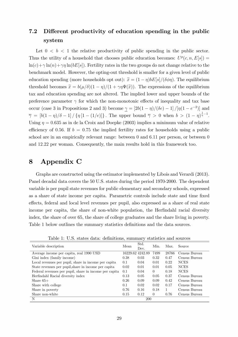
8 Appendix C

Graphs are constructed using the estimator implemented by Libois and Verardi (2013).

Panel decadal data covers the 50 U.S. states during the period 1970-2000. The dependent

variable is per pupil state revenues for public elementary and secondary schools, expressed

as a share of state income per capita. Parametric controls include state and time fixed

effects, federal and local level revenues per pupil, also expressed as a share of real state

income per capita, the share of non-white population, the Herfindahl racial diversity

index, the share of over 65, the share of college graduates and the share living in poverty.

Table 1 below outlines the summary statistics definitions and the data sources.

Table 1: U.S. states data: definitions, summary statistics and sources

Variable description MeanStd.Dev.

Min. Max. Source

Average income per capita, real 1990 USD 16229.62 4242.89 7499 28766 Census BureauGini index (family income) 0.38 0.03 0.32 0.47 Census BureauLocal revenues per pupil, share in income per capita 0.1 0.04 0.01 0.22 NCESState revenues per pupil,share in income per capita 0.02 0.01 0.01 0.05 NCESFederal revenues per pupil, share in income per capita 0.1 0.04 0 0.18 NCESHerfindahl Racial diversity index 0.13 0.05 0.05 0.37 Census BureauShare 65+ 0.26 0.09 0.09 0.42 Census BureauShare with college 0.1 0.02 0.02 0.17 Census BureauShare in poverty 0.76 0.16 0.18 1 Census BureauShare non-white 0.15 0.12 0 0.76 Census BureauN 200

29