Preliminary and incomplete.

Please do not cite without written permission from the authors.

Inequality of opportunity and economic growth:

Negative results from a cross-country analysis

Francisco H. G. Ferreira

Christoph Lakner

Maria Ana Lugo

Berk Özler1

16 June 2013

Abstract: Income differences arise from many sources. While some kinds of inequality, caused by

effort differences, might be associated with faster economic growth, other kinds, arising from unequal

opportunities for investment, might be detrimental to economic progress. We construct two new

metadata sets, consisting of 111 household surveys and 135 Demographic and Health Surveys, to revisit

the question of whether inequality is associated with economic growth and, in particular, to examine

whether inequality of opportunity has a negative effect on subsequent growth. Results are suggestive

but not robust: while overall income inequality is generally negatively associated with growth in the

household survey sample, we find no evidence that this is due to the component we attribute to

unequal opportunities. In the DHS sample, both overall wealth inequality and inequality of opportunity

have a negative effect on growth in some of our preferred specifications, but the results are not robust

to relatively minor changes. On balance, although our results are suggestive of a negative association

between inequality and growth, the data at our disposal does not permit robust conclusions as to

whether inequality of opportunity is bad for growth.

Keywords: inequality, inequality of opportunity, economic growth

JEL codes: D31, D63, O40

1 Ferreira is at the World Bank and the Institute for the Study of Labor (IZA). Lakner is at Oxford University. Lugo is

at the World Bank. Özler is at the University of Otago and the World Bank. We are grateful to Manuel Fernandez-Sierra, Marina Gindelsky, Christelle Sapata and Marc Smitz for excellent research assistance. We are also thankful to Angus Deaton, Marc Fleurbaey, Peter Lanjouw, Leonardo Santos de Oliveira and conference or seminar participants in Louvain-la-Neuve, Madrid, Rio de Janeiro, São Paulo and Washington, DC, for comments on earlier versions. The usual disclaimer applies: all remaining errors are our own. The views expressed in this paper are solely those of the authors, and do not represent those of the World Bank, its Executive Directors, or the countries they represent.

2 1. Introduction

Although the question of whether inequality may have a detrimental effect on subsequent economic

growth has been asked many times, there is no consensus answer in the literature. Theory provides

ambiguous predictions: whereas higher inequality may lead to faster growth through some channels

(such as higher aggregate savings when a greater share of income accrues to the rich), it may have

negative effects through other channels (such as lower aggregate rates of investment in human capital if

credit constraints prevent the poor from financing an optimal amount of education).

The empirical evidence has been correspondingly mixed. The earliest crop of papers including measures

of income inequality in growth regressions, in the 1990s, tended to find a negative and statistically

significant coefficient, which was widely interpreted to suggest that the theoretical channels through

which inequality was bad for growth dominated those through which there might be positive effects.

But all of these studies relied on OLS or IV regressions on a single cross-section of countries. Using the

“high-quality” subset of the Deininger-Squire dataset, which permitted panel specifications, Forbes

(2000) and Li and Zou (1998) found positive effects of lagged inequality on growth, and suggested that

omitted (time-invariant) variables may have biased the OLS coefficients. Banerjee and Duflo (2003)

raised further questions about the credibility of the earlier results – whether drawing on single cross-

sections or on panel data – by showing that if the true underlying relationship between inequality (or its

changes) and growth was non-linear, this would suffice to explain why the previous estimates were so

unstable. The prevailing conclusion from these disparate results, as summarized by Voitchovsky (2009),

was that “recent empirical efforts to capture the overall effect of inequality on growth using cross-

country data have generally proven inconclusive”. (p. 549)

And yet, the question continues to motivate researchers and policymakers alike. Asking what might

explain the absence of poverty convergence in the developing world, Ravallion (2012) revisits the effects

of the initial distribution on subsequent growth, and claims that a higher initial level of poverty – not

inequality – is robustly associated with lower economic growth. In remarks delivered at the Center for

American Progress in 2012, Alan Krueger, Chairman of the Council of Economic Advisers to the US

president, claimed that “the rise in inequality in the United States over the last three decades has

reached the point that inequality in incomes is causing an unhealthy division in opportunities, and is a

threat to our economic growth” (Krueger, 2012).2

The conjecture that an “unhealthy division of opportunities” might be bad for growth is consistent with

some of the theory: if production sets are non-convex and credit markets fail, the poor may be

prevented from choosing privately optimal levels of investment – in human or physical capital (Galor

and Zeira, 1993). Others have suggested that low levels of wealth are associated with reduced returns to

entrepreneurial effort as a result of the need to repay creditors. This moral hazard is anticipated by

lenders, leading to credit market failures and differences in the entrepreneurial opportunities available

to rich and poor agents (Aghion and Bolton, 1997).

2 Voitchovsky (2009) also suggests that the link between income and wealth inequality and growth might operate

through the distribution of opportunities: “… income or asset inequality is considered to reflect inequities of opportunity.”(p.550)

3 Drawing on the recent literature on the formal measurement of inequality of opportunity – as distinct

both from income or wealth inequality and from economic mobility – this paper seeks to address that

question directly. Is it possible that inequality – like cholesterol – comes in many varieties, and that

some are worse for the health and dynamism of an economy than others? In particular, is it possible

that the two broad categories of sources of inequality suggested by Roemer (1998) – opportunities and

efforts – have opposite effects on economic performance? If so, one reason for the ambiguity in past

empirical studies of the relationship between inequality and growth might have been the failure to

distinguish between the two types of inequality.

Unfortunately, measures of inequality of opportunity were not readily available for a large number of

countries, in the way that income inequality measures were in the Deininger-Squire dataset, or the

World Income Inequality Database of WIDER. We therefore constructed original measures of inequality

of opportunity from unit-record data from 111 income or expenditure household surveys for 36

countries, and 135 Demographic and Health Surveys (DHS) for 43 countries. These indices were

combined with information on the other explanatory variables used by Forbes (2000), which are

illustrative of the set of regressors typically used in the literature. Although we use the same Difference

GMM specification as Forbes (2000) for comparison purposes, we also draw on more recent

developments in the estimation of Generalized Method of Moments models, including a number of

System GMM specifications which are designed to alleviate the weak instruments problem that plagues

Difference GMM with highly persistent data.

A preview of our results is as follows. In neither of the two country samples – one using the income or

expenditure surveys and the other using the DHS – do we find any support for the finding in Forbes

(2000) and Li and Zou (1998) of a positive coefficient on income inequality. Instead the coefficient on

income inequality is negative in most of our specifications (including Difference GMM) and often

significantly so, raising questions about the claim that the negative signs in earlier, OLS specifications

were entirely due to time-invariant omitted variables.

However, we do not find support on these data for the hypothesis that decomposing overall income

inequality into a component associated with inequality of opportunity and a residual component

(notionally related to inequality arising from effort differences) would help resolve the inconclusiveness

of empirical estimates of the relationship between inequality and growth. In the income or expenditure

survey sample, it is the residual inequality component (driven by efforts and omitted circumstances)

that maintains a statistically significant negative coefficient in most specifications, with the inequality of

opportunity component typically insignificant. In the DHS sample the coefficient on inequality of

opportunity is generally negative, but it is only significant (at the 10% level) in one of the four preferred

specifications.

The paper is organized as follows. The next section briefly reviews the literature on the relationship

between inequality and growth, with a focus on the main empirical papers. Section 3 introduces the

concept and measurement of inequality of opportunities. Section 4 describes the econometric

specification and the data used in the analysis. Section 5 describes the estimation procedures and

presents the results. Section 6 concludes.

4 2. A brief review of the literature

Speculation that the distribution of incomes at a given point in time might affect the subsequent rate of

growth in aggregate income goes back at least to the 1950s, following the empirical finding that the

savings rate increased with income, albeit at a decreasing rate, in the Unites States (Kuznets, 1953).

Kaldor (1957) incorporated this feature into a growth model, by assuming that the marginal propensity

to save out of profits was higher than the propensity to save out of wages. Under that assumption, a

higher profit-to-wage ratio – which corresponded to higher income inequality in that model – would

lead to a faster equilibrium rate of economic growth. See also Pasinetti (1962).

But it was in the 1990s that a number of papers linking inequality to growth and the process of

development appeared, raising the profile of distributional issues not only within development

economics, but in the broader discipline as well.3 These papers came in two basic varieties: first, models

where the combination of an unequal initial distribution of wealth with imperfections in capital markets

led to inefficiencies in investment activities and, second, political economy models where inequality led

to taxation or spending decisions that deviated from those a benevolent social planner might make.

The first class of models is perhaps best illustrated by Galor and Zeira (1993), where agents have a

choice between investing in education, or working as unskilled workers. An indivisibility in the

production function of human capital and the existence of monitoring or tracking costs in the credit

markets (as a result of information and enforcement costs) implies that there is a given, positive wealth

threshold (f) below which individuals choose not to invest in schooling. Above it, all agents choose to

acquire human capital. Wealth is transmitted across generations through bequests which, under certain

assumptions render wealth dynamics a Markov process. The long-run limiting distribution depends on

initial conditions, and a higher mass of individuals below f leads to lower aggregate wealth in

equilibrium.4

Other papers involving capital market imperfections rely on alternative mechanisms, but are essentially

variations on the same theme. Banerjee and Newman (1993) model a process of occupational choices

where, in the absence of credit markets, initial wealth determines whether individuals prefer to work in

self-employment, as employees, or as employers. A nice feature of the model is that the decision also

depends on aggregate factor prices, notably the wage rate, which is endogenous to the initial wealth

distribution, leading to multiple equilibria. In Aghion and Bolton (1997) borrowers suffer from an effort

supply disincentive arising from the need to repay their debts. The strength of this moral hazard effect

increases in the size of the loan required, and thus decreases in initial wealth, leading to higher interest

rates for the poorest borrowers. A related mechanism is the choice between investing in quantity and

quality of children: poorer agents experience a lower opportunity cost from having children, and thus a

higher fertility rate. However, credit market constraints prevent them from investing as much in each

child. In the aggregate, more unequal societies (i.e. those with greater numbers of poor people for a

given mean income level) tend to have a greater relative supply of unskilled workers, and hence a lower

unskilled wage rate leading, once again, to the possibility of multiple equilibria, with higher initial

inequality possibly causing lower subsequent growth.

3 See Atkinson (1997).

4 See Loury (1981) for a precursor.

5 The second group of models focuses on the effect of inequality on policy decisions – either through

voting or through lobbying. Alesina and Rodrik (1994) and Persson and Tabellini (1994) use standard

median voter models to predict that societies with a larger gap between median and mean incomes (a

plausible measure of inequality) would choose higher rates of redistributive taxation. If taxes distort

private investment decisions, then greater inequality might lead to lower growth rates through higher

distortive taxation. Bénabou (2000) proposes an alternative set up where inequality distorts public

policy by leading to inefficiently low – rather than high – taxes. This mechanism requires that voting

power increases with wealth, so that the pivotal voter has higher than median wealth. It also requires

that public investment (e.g. educational subsidies) have positive spillovers, so that taxes finance efficient

public expenditures. These conditions are not sufficient for, but may lead to, multiple equilibria that

depend on the initial distribution.5

Inequality may also matter for political processes other than elections. Esteban and Ray (2000)

suggested that the rich may find it easier to lobby the government, and distort resource allocation from

the social optimal towards the kinds of expenditures they prefer. Campante and Ferreira (2007)

construct a model where the outcome of lobbying is generally not Pareto efficient: resource allocation

can be distorted away from the social optimal, and this may benefit poorer or richer groups, depending

on their relative productivity levels in economic and political activities.6

These various predictions have been put to the test a number of times, typically by including a measure

of initial inequality in the standard cross-country growth regression of Barro (1991). In a first phase of

the literature, both Alesina and Rodrik (1994) and Persson and Tabellini (1994) reported results from

such an exercise. Alesina and Rodrik (1994) regressed the annual growth rate in per capita GDP on the

Gini coefficients (for income or land) in 1960, for different country samples, using both OLS and two-

stage least-squares.7 Their inequality data come from secondary sources, namely compilations of

income Gini coefficients from Jain (1975) and Fields (1989), and of land coefficients from Taylor and

Hudson (1972). Both of these studies found a negative and statistically significant coefficient on initial

inequality in the growth regression. Alesina and Rodrik report a particularly robust correlation between

land inequality and subsequent growth, significant at the 1% level, and implying that an increase of one

standard deviation in land inequality would lead to a decline of 0.8 percentage points in annual growth

rates. The same basic finding of a negative effect of initial inequality on growth was reported by

Deininger and Squire (1998), using a larger (and arguably higher-quality) cross-country inequality

dataset compiled by the authors.

This Deininger-Squire dataset, introduced in the late 1990s, contained inequality data points for many

more countries and, most importantly, at various points in time. This allowed Li and Zou (1998) and

Forbes (2000) to run the same growth regression as the earlier papers on a panel, rather than a cross-

section, of countries – ushering in “Phase 2” of the literature on inequality and growth. Forbes (2000)

5 The mechanism proposed by Bénabou (2000) has the advantage that it is more consistent with the evidence that

high inequality countries tend to tax less, rather than more, than less unequal countries. See also Ferreira (2001). 6 The theoretical literature on the links between inequality and growth has been extensively reviewed, and we do

not attempt to review it comprehensively here again. For some of the best surveys, see Aghion et al. (1999), Bertola (2000) and Voitchovsky (2009). 7 Literacy rates in 1960, infant mortality rates in 1965, secondary enrollment in 1960, fertility in 1965 and an Africa

dummy are used as instruments for inequality in the TSLS first-stage.

6 reported fixed effects, random effects, and GMM estimates for a panel of 45 countries where, instead of

regressing annualized growth over a long period on a single inequality observation at the beginning of

the period, growth rates for five-year intervals were regressed on inequality at the start of each interval.

In the difference-GMM estimates, lagged values of the independent variables were used as instruments.

The results from these panel specifications were strikingly different from single cross-section results: the

coefficient on inequality was generally positive and, in the preferred specifications, statistically

significant. Various interpretations were possible: perhaps the short-run effect of inequality on growth

was positive, but the long-term effect was negative. But another, equally if not more plausible

interpretation was that the OLS cross-section coefficients were biased by omitted variables correlated

with inequality. The fixed-effects and difference GMM estimates correct at least for time-invariant

omitted variables, and this correction would appear to invalidate the negative effect of inequality on

growth.

Other estimates are also available: Barro (2000) considered the possibility that the effect of inequality

on growth might differ between rich and poor countries. While no significant relationship is found for

the whole sample, he reports a significant negative relationship for the poorer countries and a positive

relationship among richer countries when the sample is split. Voitchovsky (2005) focuses on another

kind of heterogeneity: rather than asking whether the effect differs across the sample of countries, she

tests whether inequality “at the bottom” of the distribution had a different effect from inequality “at

the top”, claiming that this would be consistent with some of the theoretical mechanisms discussed

above. Indeed she finds that inequality measures more sensitive to the bottom of the distribution

appear to have a negative effect on growth, while those more sensitive to the top of distribution are

positively associated with growth. By the early to mid-2000s, however, the dominant conclusion that

appeared to be drawn from the existing evidence was that the cross-country association between

inequality and growth was simply not robust to variations in the data or econometric specification used

to investigate it. Banerjee and Duflo (2003), for example, argue that if the true relationship between the

two variables were non-linear, it may not be identified by the linear regressions described above.

Such skepticism has not prevented a recent revival in interest in the cross-country association between

inequality and growth. In what might be described as “Phase 3” of the literature, a number of recent

papers have suggested alternative tests of the same basic idea. Easterly (2007) sets out to test the

hypothesis that, over the long term, agricultural endowments predict inequality, and inequality in turn

affects institutional development and ultimately growth.8 Using a new instrumental variable constructed

as the ratio of a country’s land endowment suitable for wheat production to the land suitable for

growing sugarcane, the author finds strong support for the endowments-inequality-growth link, with

higher inequality leading to lower subsequent growth. Berg, Ostry and Zettelmeyer (2012) look at a

different feature of growth processes – their sustainability, rather than intensity – and find that

inequality is a powerful (inverse) predictor of the duration of future growth spells. Ravallion (2012) also

finds that features of the initial distribution affect future growth, but suggests that poverty - rather than

inequality - provides the best distributional predictor of future growth.

8 This hypothesis was originally formulated in these terms by Engerman and Sokoloff (1997).

7 Another possibility raised in this latest phase of research into the link between distribution and

economic performance is that scalar measures of income or expenditure inequality may be composite

indicators, the constituent elements of which affect economic performance in different ways. In

particular, it has been suggested that inequality of opportunity might have more adverse consequences

than the inequality which arises from differential rewards to effort (e.g. Bourguignon, Ferreira and

Walton, 2007). This claim resonates with some of the theoretical mechanisms reviewed above, for

example that low wealth leads to forgone productive investment opportunities for part of the

population. Such mechanisms operate through differences in the opportunity sets faced by different

agents, and are potentially still consistent with the differences in earnings providing incentives for

effort, which might be good for growth.

If overall income inequality comprises both inequality of opportunity and inequality due to effort, and

these two components have different effects on economic growth, then the relationship that has

typically been estimated is mis-specified, and one ought to distinguish between the two kinds of

inequality. Marrero and Rodriguez (forthcoming) do this for 26 states of the United States: they

decompose a Theil (L) index into a component associated with inequality of opportunity and another

which they attribute to differences in efforts. When economic growth is regressed on income inequality

and the usual control variables in their sample of states, the coefficient on inequality is statistically

insignificant. But when the two components of inequality are entered separately, the coefficient on

“effort inequality” is generally positive, and that on inequality of opportunity is negative and strongly

significant.

To our knowledge, Marrero and Rodriguez (forthcoming) is the only paper that investigates whether

inequality of opportunity is the “active ingredient” in the relationship between inequality and growth.

Their findings suggest that this component of inequality was negatively associated with economic

growth in the United States in the 1970-2000 period. Is this a more general result? Can be the same be

said of other places and contexts? In particular, can a decomposition of inequality into an opportunity

and a residual component help resolve the inconclusiveness of the cross-country literature on this

subject? In order to address this question, the next section briefly reviews the recent empirical literature

on the measurement of inequality of opportunity, and defines the indices we use in this paper.

3. Inequality of opportunity

The concept of equality of opportunity has been widely discussed among philosophers since the seminal

papers by Dworkin (1981), Arneson (1989) and Cohen (1989). It is central to the school of thought that

believes that meaningful theories of distributive justice should take personal responsibility into account.

In essence, these “responsibility-sensitive” egalitarian perspectives propose that those inequalities for

which people can be held ethically responsible are normatively acceptable. Other inequalities,

presumably driven by factors over which individuals have no control, are unacceptable, and often

referred to as inequality of opportunity.

8 The concept was formalized and introduced to economists by Roemer (1993, 1998) and van de Gaer

(1993). Among economists, its usage was initially restricted to social choice theorists. Broader

applications in the field of public economics began with Roemer et al. (2003), who investigate the

effects of fiscal systems – broadly the size and incidence of taxes and transfers – on inequality of

opportunity in eleven (developed) countries. Actual empirical measures of inequality of opportunity

based on the definitions provided by Roemer (1998) and van de Gaer (1993) are more recent, and

include Bourguignon et al. (2007), Lefranc et al. (2008), Checchi and Peragine (2010) and Ferreira and

Gignoux (2011).

In this paper, we follow the ex-ante approach independently proposed by Checchi and Peragine (2010)

and Ferreira and Gignoux (2011). Consider a population of agents indexed by . Let yi denote

what is known in this literature as the “advantage” of individual i which, in the present paper, will be a

measure of household income, consumption, or wealth. The N-dimensional vector y denotes the

distribution of incomes in this population. Let Ci be a vector of characteristics of individual i over which

she has no control, such as her gender, race or ethnic group, place of birth, and the education or

occupation of her parents. Let Ci have J elements, all of which are discrete with a finite number of

categories, xj, Following Roemer (1998), the elements of Ci are referred to as circumstance

variables.

Define a partition of the population , such that ,

, and Each element of Tk, is a subset of the

population made up of individuals with identical circumstances. Following Roemer (1998), we call these

subgroups “types”. The maximum possible number of types is given by .9

In simple terms, the ex-ante approach to measuring inequality of opportunity consists of agreeing on a

measure of the value of the opportunity set facing each type, assigning each individual the value of his

or her type’s opportunity set, and computing the inequality in that distribution.10 Following van de Gaer

(1993) and Ooghe et al (2007), Ferreira and Gignoux (2011) choose the mean income in type k, , as a

measure of the value of the opportunity set faced by people in that type. In other words, a hypothetical

situation of equality of opportunity would require that:

(1)

Using the superscript k to indicate the type to which individual i belongs, a typical element of the

income vector y is denoted . The counterfactual distribution in which each individual is assigned the

value of his or her opportunity type is then simply the smoothed distribution corresponding to the

vector y and the partition П, i.e the distribution obtained by replacing with , .11 Denoting that

distribution as , Ferreira and Gignoux propose a very simple measure of inequality of opportunity,

9 if some cells in the partition are empty in the population.

10 The ex-post approach to the measurement of inequality of opportunity requires computing the inequality among

individuals exerting the same degree of effort which, in turn, requires assumptions about how effort can be measured. See Fleurbaey and Peragine (2012) for a discussion of both approaches. 11

See Foster and Shneyerov (2000).

KTTT ,...,, 21 NTTT K ,...,1...21

klTT kl ,, .,,,, kTjTijiCC kkji

J

j

jxK1

KK

9

namely , where I() is the mean logarithmic deviation, also known as the Theil (L) index. Among

inequality indices that use the arithmetic mean as the reference income, this measure is the only one

that satisfies the symmetry, transfer, scale invariance, population replication, additive decomposability

and path-independent decomposability axioms (Foster and Shneyerov, 2000). This is the empirical

measure of inequality of opportunity used in the income and expenditure survey sample in Section 5

below.

The mean log deviation is not, however, suitable for use in the Demographic and Health Survey sample.

As discussed in the next section, the DHS surveys do not contain credible measures of income or

consumption. It does however contain information on a number of assets and durable goods owned by

the household, as well as dwelling and access to service characteristics. Following Filmer and Pritchett

(2001), it has become standard practice to use a principal component of these variables as a proxy for

household wealth. As a principal component, this wealth index has negative values, and its mean is zero

by construction, so that the mean log deviation is not a suitable measure of its dispersion.

In our DHS sample, we therefore follow Ferreira et al. (2011) in using the variance of predicted wealth

from an OLS regression of the asset index on all observed circumstances in C as our measure of

inequality of opportunity. The essence of the rationale for this choice of measure is as follows.12 We

tend to think of advantage (in this case the wealth index w) as a function of circumstances, efforts, and

possibly some random factor u:

(2)

Although circumstances are exogenous by definition (i.e. they are factors beyond the control of the

individual and are hence determined outside the model), efforts can be influenced by circumstances:

(3)

For the purposes of simply measuring inequality of opportunity (as opposed to identifying individual

causal pathways), it suffices to estimate the reduced form of the system (2)-(3). Under the usual

linearity assumption, this is given by:

(4)

Under this linearity assumption, - where - is a parametric equivalent to the smoothed

distribution previously described. It is a distribution where individual values of the wealth index

have been replaced by the mean conditional on circumstances, much as before. Whereas a non-

parametric approach, using the cell means, is clearly preferable when data permits it, the parametric

approach based on estimating the reduced-form equation (4) may be preferable when K is large relative

to N, so that many cells are sparsely populated, and their means imprecisely estimated. Given the

properties of the distribution of w, we follow Ferreira et al. (2011) in measuring its inequality simply by

the variance: .

12

This discussion draws heavily on Bourguignon et al. (2007) and Ferreira and Gignoux (2011). Readers are referred to those papers for detail.

10 An important caveat about these measures is that, in practice, not all relevant circumstance variables

may be observed in the data. If the vector of observed circumstances has dimension less than J, then

both the non-parametric index and the parametric measure are lower-bound estimates

of true inequality of opportunity. See Ferreira and Gignoux (2011) for a formal proof. In addition, in the

presence of omitted circumstances, clearly neither the non-parametric decomposition nor the reduced-

form regression (4) can be used to identify the effect of individual circumstance variables. We do know

the direction of bias – downward – for the overall measures of inequality of opportunity, however,

which is why they are lower-bound estimators.

4. Data and econometric specification

Our aim in this paper is to investigate whether decomposing inequality into inequality of opportunity

and a residual term (comprising inequality arising from efforts, as well as omitted circumstances) helps

resolve the inconclusiveness about the effects of inequality on subsequent growth in the empirical

cross-country literature. To this end, we start from the panel specification of Forbes (2000):

(5)

Different versions of this equation are estimated in the income/expenditure survey sample, and in the

DHS sample. In both cases, the dependent variable, , is the average annual growth rate of per capita

gross national income in a five-year interval. The data comes from the World Bank’s World Development

Indicators data set, from which we also obtain the (five-year) lagged national income per capita, ,

expressed in constant 2000 US dollars.13 – our measure of overall inequality – is the key

variable that varies between the two samples: it denotes the mean logarithmic deviation of incomes (or

expenditures) at the beginning of the five-year interval, in the income/expenditure survey sample. In the

DHS sample, it denotes the (overall) variance of the asset index ( ), also at the beginning of the five-

year interval. Unlike in Forbes (2000) or indeed, to our knowledge, any previous paper in this literature,

these inequality indices do not come from a compilation of scalar measures from earlier studies, such as

Deininger-Squire database, or the WIDER World Income Inequality Database. Instead, the inequality

indices are computed from the original microdata for all surveys in all countries. Details on the meta

household-level data set are provided below.

Female and male education data come from Lutz et al. (2007, 2010), and is represented by the

proportion of adult (male/female) population that attained at least one year of secondary education.

Lutz and co-authors produced estimates for 120 countries from 1970 to 2010, on a quinquennial basis.

These data are in the spirit of Barro and Lee (2001), although the method used to complete missing data

differ slightly.14 Finally, as in Forbes, market distortions are proxied by the price level of investment,

from Penn World Tables (version 6.3), defined as the purchasing power parity of investment/exchange

rate ( ).

13

With the exception of Haiti, where GDP is used instead of GNI. 14

While Barro and Lee used the perpetual inventory method to complete their data set, and transform flux into stock of education, Lutz et al. used backward (2007) and forward (2010) projections from empirical observations given by UNESCO and UN data on population structure.

11 After reporting results for (5), where inequality enters as a composite indicator, we re-estimate this

equation replacing with our measures of inequality of opportunity: in the income

expenditure survey sample, and in the DHS sample. For simplicity, we denote both of these as

in the generic specification. We also include the residual term, ,

and estimate:

(6)

Equations (5) and (6) were estimated using a variety of panel methods, including fixed effects, random

effects, Difference GMM (Arellano and Bond, 1991), and System GMM (Arellano and Bover, 1995;

Blundell and Bond, 1998), with the appropriate modifications. We do not report results from the fixed

effects estimation, given that the lagged dependent variable on the RHS of these equations is likely to

render that specification subject to endogeneity bias. In the next section, we discuss results from various

different GMM specifications.

In the remainder of this section, we briefly describe the microdata sets used to compute the inequality

and inequality of opportunity variables. The availability of household survey micro-data with

information on both a reliable indicator of well-being (income, consumption or wealth) and

circumstance variables – which are required for computing inequality of opportunity measures – is the

key factor constraining our sample(s) of countries. The requirement is even more stringent since we

need, for each country, at least two comparable surveys five years apart to construct the panel of

countries – three when using GMM estimators. As noted earlier, we use two types of household

surveys: income or expenditure households surveys (HHS) such as labor force surveys, household budget

surveys or Living Standard Measurement Surveys, in the first country sample, and Demographic and

Health Surveys (DHS) in the second country sample.

The HHS sample contains 36 countries, both developed and developing. For a large proportion of the

countries, we use three harmonized meta-databases that construct comparable measures of household

income or consumption. We use the Luxembourg Income Study (LIS) for 20 (mostly developed)

countries, the Socioeconomic Database for Latin America and the Caribbean (SEDLAC) for seven Latin

American countries, and the International Income Distribution Database from the World Bank (I2D2) for

another six developing economies. For the remaining 3 countries included in the sample, we use the

respective national household surveys.15 The advantage variable used to compute total inequality and

inequality of opportunity is always a measure of household well-being. For 28 countries, it is net

household income per capita, while for another eight, where reliable income data is not available, it is

household per capita expenditure. Definitions are always consistent within countries and a dummy

variable indicating whether the inequality measure is based on expenditure or incomes is included in the

estimation of the growth model.

In all countries, a single circumstance variable was used to partition the population into types, namely

social origin (J=1). The specific indicator of social origin varies across countries, however, depending on

data availability. Race or ethnicity is used whenever available, but language spoken at home, religion,

caste, nationality of origin, immigration status and region of birth are also used. The number of types (K) 15

For the United States, three observations (1974, 1979, and 1986) come from LIS harmonized database (based on the Current Population Survey -CPS), and for the remaining four (1991, 1995, 2000, 2005) we use directly the CPS.

12 resulting from the partition ranges between 2 and 6 across countries. Once again, the circumstance

variables and the number of types are unchanged over time within countries. Table A1 in the appendix

provides more detailed information on the source and years of the household survey, the welfare and

circumstance variables and the number of types in the partition for each country.

The use of a single circumstance variable, social origin, is potentially a serious limitation of this study.

Most studies of inequality of opportunity within specific countries draw on a richer set of circumstance

variables including father’s and or mother’s education and occupation and region of birth, in addition to

race or language spoken at home. When the advantage variable is individual earnings, rather than

household income or expenditure, gender is typically also included.16 The resulting partition typically

contains a much larger number of types: 72 in Checchi and Peragine (2010) and Belhaj-Hassine (2012),

54 or 108 in Ferreira and Gignoux (2011), and so on. Naturally, a higher dimension (J) for the

circumstance vector (C) allows the analyst to better capture the possible sources of inequality of

opportunity. Although the resulting measure is still a lower-bound on actual inequality of

opportunity, as noted earlier, fewer omitted circumstances is likely to mean a smaller underestimation

of I.Op.

We were unable to work with additional circumstances because data were not available on them in a

sufficient number of household surveys. This was particularly true of information on parental education

and occupation, which is seldom included for a representative sample of adults. Since these family

background variables have typically been found to account for a substantial share of the between-type

inequality in other studies, we anticipate the cost of having to rely on a “lowest common denominator”

circumstance vector for the cross-country analysis to be non-trivial.

In an attempt to address this problem, we extended our analysis to an additional sample of countries

and household surveys, by drawing on the Demographic and Health Surveys (DHS), where additional

circumstance variables were available. The DHS sample contains 43 developing countries from Africa,

Asia and Latin America (see table A2 in the Appendix for details). The earliest survey used is from 1986

and the most recent from 2006. The DHS are designed to provide in-depth information on health,

nutrition, and fertility. In addition, the survey includes socioeconomic information of household

members and access to services. As noted earlier, the DHS does not typically contain estimates of

household income or expenditure, so we construct a wealth index as the first principal component of a

set of indicators on assets and durable goods owned, dwelling characteristics, and access to basic

services. The list of indicators included may vary somewhat from country to country, but we maintain

the same set of variables within countries across time.

For all women aged 15 to 49, the DHS collects relatively detailed information on circumstance variables.

We define the types based on the following indicators: region of birth, number of siblings, religion,

ethnicity, race, mother’s education and father’s education. Since not all indicators are available in all

surveys and the number of categories in each variable also varies, the number of types differs from

16

Gender is not generally included when the advantage variable is defined at the household-level because the gender of household head is, at least in principle, an endogenous decision for individuals, and hence not a circumstance.

13 country to country (but remains the same within countries across time). These numbers are also

reported in Table A2.

5. Estimation and Results

We first discuss the results from the income and expenditure surveys (HHS). Table 1 reports estimates of

equation (5) using total inequality measures from this sample. Because of the presence of the lagged

dependent variable on the right-hand-side, coefficients from the fixed-effects specification are likely to

be biased, and are not reported. They are available from the authors on request and, as we shall see,

including them would not alter the substance of our conclusions. The first column in Table 1 reports the

Difference GMM estimation corresponding to the preferred specification in Forbes (2000). As in her

paper, we find evidence of conditional convergence, but the other results are substantially different. In

particular, whereas Forbes (2000) reports a coefficient on lagged inequality that is positive and

significant, our estimate for (-0.084) is negative and significant at the 10% level.

This difference likely reflects differences in the country and period coverage of the two samples. We

have 111 surveys for 36 countries, whereas Forbes has 135 surveys (in the GMM specification) for 45

countries. Twenty-two countries are present in both Forbes’s and our HHS sample. Periods also differ,

with Forbes using Gini coefficients between 1961-65 and 1986-1990, whereas our sample ranges from

1982-1986 and 2002-2006. Clearly, neither sample of countries is representative of the world, since they

are driven entirely by survey availability, which is evidently non-random. Although our sample covers

fewer countries, it has slightly broader regional coverage: for example, we have three African countries,

whereas Forbes’s sample has none. In addition, as noted earlier, our inequality measures satisfy a higher

standard of international comparability, since they are all computed under exactly the same criteria and

using the same routines directly from the microdata, whereas Forbes (2000) relied on Gini coefficients

from the Deininger-Squire data set.

Estimation of GMM models has evolved since the year 2000. Considerable concern has been expressed,

for example, that in a context where the time series are persistent and the time dimension is small “the

first-differenced GMM estimator is poorly behaved” (Bond et al. 2001). In particular, under those

circumstances - which evidently apply to the data used in this paper, in Forbes (2000), and most of the

cross-country growth literature - the two-period lagged dependent-variable (in levels) used as

instruments for the first-differences in the second stage are weak instruments. When instruments are

weak, large finite sample biases can occur, and these problems have been documented in the context of

first-difference GMM models (Blundell and Bond, 1998; Bond et al. 2001).

Columns 2-4 in Table 1 therefore report results from the alternative “System GMM” estimation. Under

an additional set of moment restrictions, system GMM models combine the usual equation in first-

differences using lagged levels as instruments, with an additional equation in levels, using lagged first-

differences as instruments. According to Blundell and Bond (1998), Blundell et al. (2000) and Bond et al.

(2000), this approach results in substantial reductions in finite-sample biases in Monte-Carlo

experiments. Although system GMM estimation is, for these reasons, now generally preferred to

difference GMMs, it is not problem-free. In particular, Roodman (2009) urges caution with the effect of

instrument proliferation on the Hansen test of joint validity of instruments. Although a Hansen statistic

14 below 0.25 typically suggests that instruments may not be valid, Roodman points out that values of (or

very close to) 1.0 suggest that the Hansen test is no longer informative. Two alternative approaches to

limiting the instrument set have been found to help restore power to the Hansen test: collapsing the

instrument set along the time dimension, or using principal components of the full instrument set.

Column (2) reports on the specification using the full set of instruments; while column (3) uses principal

component analysis to aggregate all instruments into a smaller number of components. Column (4)

combines these two techniques.

The negative sign of the coefficient on overall inequality in the Difference GMM remains in two of the

system GMM specifications, although it is only significant in column (3). The coefficient is positive and

insignificant in specification (4). The Hansen statistic is 1.00 both for the Difference GMM and the

System GMM with full instruments, suggesting that instrument proliferation is weakening the test. On

that basis, columns (3) and (4) should be the preferred specification on this Table. They suggest that

lagged income inequality is not positively associated with subsequent growth. The negative association

from the difference GMM survives in one case, but is not robust to changes in the estimation procedure.

Our main interest, however, lies in examining whether and how the association between inequality and

growth might change when we decompose overall inequality into the opportunity and residual

components, and respectively, by estimating equation (6). Tables 2 and 3 report results

from this regression on the HHS country sample. Table 2 reports the standard (one-step) GMM for the

four specifications used in Table 1: difference; system with the full instrument set; system with a

principal component of instruments; and system when the principal component of instruments is

further collapsed. Because our data set contains a few “interval gaps” (i.e. five-year intervals for which

we have no surveys, between five-year intervals for which we do), we re-estimate each of the

specifications in Table 2 using also the forward orthogonal deviations method, suggested by Arellano

and Bover (1995). This estimator transforms the data by removing the average of all available future

observations, and has the advantage of being unaffected by gaps in the data. Results are presented in

Table 3.

The difference GMM estimates, both following the one-step method and using forward orthogonal

deviations, are consistent with a negative association between lagged inequality of opportunity and

growth, although only at the 10% level. The residual component is statistically insignificant in both cases

so that, if one restricted one’s attention exclusively to the preferred specification in Forbes (2000), one

might conclude that there was some support, albeit at low levels of significance, for the hypothesis that

it is inequality of opportunity that accounts for the negative association between income inequality and

growth. But the possibility of weak instrument biases, and a Hansen statistic of 1.00 in both cases,

argues for a robustness test with system GMM. The negative association between inequality of

opportunity and growth clearly fails this robustness test. In fact, in five of the six specifications in

columns (2)-(4) of Tables 2 and 3, it is the coefficient on the residual inequality component that is

negative and, in all cases, statistically significant at the 5% level or lower.17 While these results are not

inconsistent with – and possibly offer some support for – the suggestive evidence from Table 1 that

17

It is also interesting that none of the other explanatory variables – male and female education, and price distortions – is significant in these system GMM specifications.

15 overall income inequality is negatively associated with growth, they are clearly not supportive of the

hypothesis that there might be a stronger negative association between inequality of opportunity and

growth.

We considered the possibility that these findings might be driven by measurement error. As noted in

Section 4, the need for (rough) comparability of circumstance sets across countries led to a measure of

inequality of opportunity based on a very sparse partition of types. Like other examples of this method,

the measure used in the regressions reported in Tables 2 and 3 is a lower-bound indicator. But given the

paucity of types, it is arguably a very substantial underestimate of true inequality of opportunity. While

it is evidently not the only possible cause, this kind of measurement error would certainly be consistent

with substantial amounts of inequality of opportunity (due to omitted circumstances) contaminating the

residual component, leading to biased coefficients.

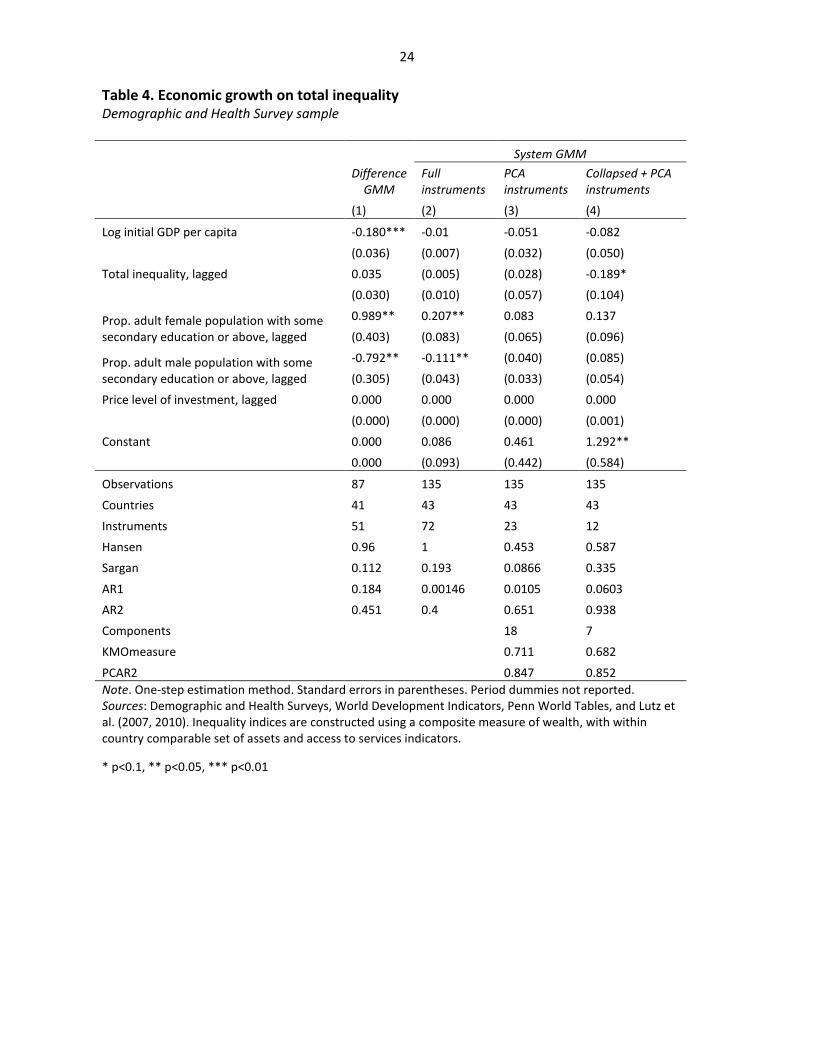
Given the data limitations in the HHS sample, we therefore turned to the DHS sample, as previously

described. DHS samples contain information on a richer set of circumstances, as noted earlier, and

therefore lead to a greater number of types in most countries. Table 3, which is analogous to Table 1,

reports the results of estimating equation (5) on this sample of countries. The coefficient on total

inequality, now measured by the variance of the wealth index, is statistically insignificant in the

difference GMM specification (column 1) and in the system GMM specification with full instruments

(column 2). Very high Hansen statistics suggest both of these columns should be treated with

circumspection. Columns (3) and (4), which reduce the instrument set by means of a principal

component analysis (and collapsing), have Hansen statistics in a much more acceptable range (0.45 –

0.59). Total inequality is negative and significant at 10% in one of them, and remains insignificant in the

other.

When overall inequality in the wealth index is decomposed into a component due to inequality of

opportunities and a residual, in Tables 5 and 6, coefficients on both and are statistically

insignificant in the difference GMM specification and in the system GMM with full instruments (columns

1 and 2).18 Once again, the possibility of weak instrument biases and Hansen statistics near 1.00 suggest

caution in interpreting these findings. We prefer the specifications in columns (3) and (4). In those

columns, the coefficient on inequality of opportunity is always negative, but it is only statistically

significant in one case (column 4 in Table 6). And in that specification, the residual component of

inequality is also negative and significant.

Other independent variables are also seldom significant in the specifications with reduced instrument

sets. The main exception is the usual conditional convergence result of a negative coefficient on lagged

income. In column (3) of Table 5, female secondary education is positive and significant at 10%, but male

secondary education is negative and significant at 10%.

6. Conclusions

Our motivating hypothesis was that the lack of robust conclusions about the association between lagged

inequality and economic growth in the previous literature might have been driven, at least in part, by

18

Analogously to Tables 2 and 3 for the HHS sample, Table 5 uses the standard one-step GMM procedure, while Table 6 uses the forward orthogonal deviations method.

16 the conflation of two different kinds of inequality into the conventional income inequality measure:

inequality of opportunities and inequality driven by efforts. Because efforts are notoriously difficult to

measure, we have followed the recent literature on the measurement of ex-ante inequality of

opportunity, and decomposed overall income inequality into a component associated with

opportunities, and a residual component, driven by efforts as well as omitted circumstances.

These decompositions were carried out for the mean log deviation of household per capita incomes (or

expenditures) in 111 household income and expenditure surveys for 36 countries, and for the variance

of a wealth index obtained from Demographic and Household Surveys in 135 surveys for 42 countries.

The resulting indices of inequality of opportunity and residual inequality were then included as right-

hand side variables in growth regressions that also included measures of male and female human capital

investment and a measure of investment price distortion, following the Forbes (2000) specification. The

same regressions were run for the overall income inequality measure (with no decomposition). The two

country-level samples were unbalanced panels with a minimum time dimension of three periods, so we

relied on the Generalized Method of Moments for estimation. Given concerns about weak-instrument

biases in the first-difference GMM, various system GMM specifications we were also used.

Our two main findings are as follows. First, although the suggestive evidence of a negative association

between overall income inequality and subsequent growth in our data is not robust to all changes in

specification, it does appear possible to rule out a positive association such as the one found by Forbes

(2000) and Li and Zou (1998). The coefficient on lagged overall inequality is generally negative and, it is

always negative in those instances when it is significant.

Second, the evidence in support of our original hypothesis is extremely weak. In the HHS sample, it is

actually the residual component of inequality that is negatively and significantly associated with

subsequent growth (which adds weight to the first point above). In the DHS country sample, the

coefficient on inequality of opportunity is generally negative, but only significant in one of the four

“preferred” specifications. These are negative results, in that they certainly do not allow us to reject the

null hypothesis of no effect of I.Op. on growth. But neither can we confidently accept that null

hypothesis, particularly given the prevalence of measurement error in the inequality of opportunity

variable.

It does not appear, at least for these samples of countries and in the period from the 1980s to the mid-

2000s, that inequality is positively associated with growth, as some of the earlier literature suggested. It

is more likely that this association is negative, although not robust. If that relationship is driven by a

particular kind of inequality, such as inequality of opportunity, this cannot be inferred from the available

cross-country data, despite considerable advances in its availability.

17

References

Aghion, Philippe and Patrick Bolton (1997): “A theory of trickle-down and development”, Review of

Economic Studies 64: 151-172.

Aghion, Philippe, Eve Caroli and Cecilia Garcia-Peñalosa (1999): “Inequality and economic growth:

The perspective of the new growth theories”, Journal of Economic Literature 37: 1615-1660.

Alesina, Alberto and Dani Rodrik (1994): “Distributive politics and economic growth”, Quarterly

Journal of Economics 109: 465-490.

Arellano, Manuel and Stephen Bond (1991): "Some Test of Specification for Panel Data: Monte Carlo

Evidence and an Application to Employment Equations." Review of Economic Studies 58(2): 277–

97.

Arellano, Manuel and Olympia Bover (1995): “Another look at the instrumental variable estimation

of error-component models”, Journal of Econometrics 68: 29-52.

Arneson, Richard (1989): "Equality of Opportunity for Welfare," Philosophical Studies: An

International Journal for Philosophy in the Analytic Tradition, 56 (1), 77-93.

Atkinson, Anthony (1997): “Bringing income distribution in from the cold”, Economic Journal 107:

297-321.

Banerjee, Abhijit and Esther Duflo (2003): “Inequality and growth: What can the data say?”, Journal

of Economic Growth 8: 267-299.

Banerjee, Abhijit and Andrew Newman (1993): “Occupational choice and the process of

development”, Journal of Political Economy 101 (2): 274-298.

Barro, Robert (1991): “Economic growth in a cross section of countries”, Quarterly Journal of

Economics 106(2): 407-443.

Barro, Robert (2000): "Inequality and Growth in a Panel of Countries." Journal of Economic Growth

5(1):5–32.

Barro, Robert and Jong-Wha Lee (2001): "International Data on Educational Attainment: Updates

and Implications." Oxford Economic Papers 53(3): 541–63.

Belhaj-Hassine, Nadia (2012): “Inequality of Opportunity in Egypt”, World Bank Economic Review 26

(2): 265-295.

Bénabou, Roland (2000): "Unequal Societies: Income Distribution and the Social Contract." American

Economic Review 90(1): 96–129.

Berg, Andrew, Jonathan Ostry and Jeromin Zettelmeyer (2012): “What makes growth sustained?”,

Journal of Development Economics 98: 149-166.

18

Bertola, Giuseppe (2000): “Macroeconomics of Distribution and Growth”, Chapter 9 in A.B. Atkinson

and F. Bourguignon (eds) Handbook of Income Distribution, vol.1 (Amsterdam: Elsevier North

Holland).

Blundell, Richard and Stephen Bond (1998): “Initial conditions and moment restrictions in dynamic

panel data models”, Journal of Econometrics 87(1): 115-143.

Blundell, Richard, Stephen Bond and F. Windmeijer (2000): “Estimation in dynamic panel data

models: improving on the performance of the standard GMM estimator”, in B. Baltagi (ed.)

Nonstationary Panels, Panel Cointegration and Dynamic Panels (Amsterdam: Elsevier Science).

Bond, Stephen, Anke Hoeffler and Jonathan Temple (2001): “GMM estimation of empirical growth

models”, CEPR Discussion Paper No. 3048, London, England.

Bourguignon, François, Francisco H. G. Ferreira and Marta Menéndez (2007): “Inequality of

opportunity in Brazil”, Review of Income and Wealth 53 (4): 585-618.

Bourguignon, François, Francisco H. G. Ferreira and Michael Walton (2007): “Equity, efficiency and

inequality traps: A research agenda”, Journal of Economic Inequality 5: 235-256.

Campante, Filipe and Francisco H. G. Ferreira (2007): “Inefficient lobbying, populism and oligarchy”,

Journal of Public Economics 91: 993-1021.

Checchi, Daniele and Vito Peragine (2010): "Inequality of Opportunity in Italy," Journal of Economic

Inequality, 8 (4): 429-450.

Cohen, Gerry (1989): "On the Currency of Egalitarian Justice," Ethics 99 (4): 906-944.

Deininger, Klaus and Lyn Squire (1998): "New Ways of Looking at Old Issues: Inequality and Growth."

Journal of Development Economics 57(2): 259–87.

Dworkin, Ronald (1981): "What is Equality? Part 2: Equality of Resources”. Philosophy and Public

Affairs, 10 (4): 283-345.

Easterly, William (2007): “Inequality does cause underdevelopment: Insights from a new

instrument”, Journal of Development Economics 84: 755-776.

Engerman, Stanley and Kenneth Sokoloff (1997): "Factor Endowments, Institutions, and Differential

Paths of Growth Among New World Economies: A View from Economic Historians of the United

States." in Stephen Haber, eds., How Latin America Fell Behind. Stanford, C.A.: Stanford

University Press.

Esteban, Joan Maria and Debraj Ray (2000): “Wealth constraints, lobbying, and the efficiency of

public allocation”, European Economic Review, 44: 694-705.

Ferreira, Francisco H. G. (2001): "Education for the Masses? The Interaction between Wealth,

Educational and Political Inequalities." Economics of Transition 9(2): 533–52.

19

Ferreira, Francisco and Jèrèmie Gignoux (2011): “The measurement of inequality of opportunity:

Theory and an application to Latin America”, Review of Income and Wealth 57 (4): 622-657.

Ferreira, Francisco, Jèrèmie Gignoux and Meltem Aran (2011): “Measuring inequality of opportunity

with imperfect data: the case of Turkey”, Journal of Economic Inequality 9: 651-680.

Fields, Gary (1989): “A compendium of data on inequality and poverty for the developing world”,

Cornell University; unpublished manuscript.

Filmer, Deon and Lant Pritchett (2001): “Estimating Wealth Effects without Expenditure Data – or

Tears: An application to educational enrollments in states of India”, Demography, 38(1): 115-

132.

Fleurbaey, Marc and Vito Peragine (2012): "Ex Ante versus Ex Post Equality of Opportunity,"

Economica.

Forbes, Kristin (2000): “A reassessment of the relationship between inequality and growth”,

American Economic Review 90 (4): 869-887.

Foster, James and Artyom Shneyerov (2000): "Path Independent Inequality Measures," Journal of

Economic Theory 91 (2): 199-222.

Galor, Oded and Joseph Zeira (1993): “Income distribution and macroeconomics”, Review of

Economic Studies 60: 35-52.

Jain, Shail (1975): “Size distribution of income: a comparison of data”, The World Bank; unpublished

manuscript.

Kaldor, Nicholas (1957): “A model of economic growth”, Economic Journal LXVII: 591-624.

Krueger, Alan (2012): “The rise and consequences of inequality in the United States”, Remarks

delivered to the Center for American Progress, Washington, DC (January 12, 2012).

Kuznets, Simon (1953): Shares of upper-income groups in income and savings, National Bureau of

Economic Research, New York.

Lefranc, Arnaud, Nicolas Pistolesi and Alain Trannoy (2008): "Inequality of Opportunities vs.

Inequality of Outcomes: Are Western Societies All Alike?" Review of Income and Wealth 54(4):

513-546.

Li, H. Y. and H. F. Zou (1998): “Income Inequality is not Harmful for Growth: Theory and Evidence”,

Review of Development Economics 2: 318-334.

Loury, Glenn (1981): “Intergenerational Transfers and the Distribution of Earnings”, Econometrica

49: 843-867.

20

Lutz, Wolfgang, Anne Goujon, Samir K.C. and Warren Sanderson (2007) “Reconstruction of

populations by age, sex and level of educational attainment for 120 countries for 1970-2000”,

Vienna Yearbook of Population Research 2007: 193-235

Lutz, Wolfgang, Samir KC, Bilal Barakat, Anne Goujon, Vegard Skirbekk, and Warren Sanderson

(2010) “Projection of populations by level of educational attainment, age, and sex for 120

countries for 2005-2050”, Demographic Research 22: 383-472.

Marrero, Gustavo and Juan Gabriel Rodríguez (forthcoming): “Inequality of Opportunity and

Growth”, Journal of Development Economics.

Ooghe, Erwin, Erik Schokkaert and Dirk van de Gaer (2007): “Equality of Opportunity versus Equality

of Opportunity Sets”, Social Choice and Welfare 28: 209-230.

Pasinetti, Luigi (1962): “Rate of profit and income distribution in relation to the rate of economic

growth”, Review of Economic Studies 29: 267-279.

Persson, Torsten and Guido Tabellini (1994): “Is inequality harmful for growth?” American Economic

Review 84: 600-621.

Ravallion, Martin (2012): “Why don’t we see poverty convergence?”, American Economic Review

102 (1): 504-523.

Roemer, John (1993): "A pragmatic theory of responsibility for the egalitarian planner," Philosophy

and Public Affairs 22 (2): 146-166.

Roemer, John (1998): Equality of Opportunity, Harvard University Press, Cambridge.

Roemer, John et al. (2003): “To what extent do fiscal regimes equalize opportunities for income

acquisition among citizens?” Journal of Public Economics 87: 539-565.

Roodman, David (2009): “A note on the theme of too many instruments”, Oxford Bulletin of

Economics and Statistics 71: 135-158.

Taylor, C. L. and M. C. Hudson (1972): World Handbook of Political and Social Indicators, 2nd ed. New

Haven, CT: Yale University Press.

Van de Gaer, Dirk (1993): Equality of Opportunity and Investment in Human Capital, Ph.D.

dissertation, Catholic University of Louvain, 1993.

Voitchovsky, Sarah (2005): “Does the profile of income inequality matter for economic growth?”,

Journal of Economic Growth 10: 273-296.

Voitchovsky, Sarah (2009): “Inequality and Economic Growth”, Chapter 22 in W. Salverda, B. Nolan

and T. Smeeding (eds.) The Oxford Handbook of Economic Inequality. Oxford, OUP.

21

Table 1. Economic growth on total inequality

Income/expenditure survey sample

Difference GMM

System GMM

Full instruments PCA instruments

Collapsed + PCA instruments

(1) (2) (3) (4)

Log initial GDP per capita -0.228*** -0.003 -0.008 -0.034

(0.040) (0.006) (0.016) (0.051)

Total inequality, lagged -0.084* -0.032 -0.143*** 0.551

(0.045) (0.027) (0.051) (0.649)

Prop. adult female population with some secondary education or above, lagged

-0.661 0.052 -0.034 0.070

(0.548) (0.082) (0.227) (1.692)

Prop. adult male population with some secondary education or above, lagged

1.085 -0.021 0.081 0.217

(0.687) (0.094) (0.356) (2.196)

Price level of investment, lagged 0.001* -0.001** -0.000 -0.004

(0.001) (0.000) (0.001) (0.005)

Constant

0.092* 0.160* 0.393

(0.046) (0.093) (0.383)

Observations 75 111 111 111

Countries 36 36 36 36

Instruments 58 80 30 15

Hansen 1.000 1.000 0.695 0.750

Sargan 0.0463 0.0946 0.269 0.875

AR1 0.965 0.585 0.480 0.568

AR2 0.170 0.207 0.175 0.185

Components

25 8

KMOmeasure

0.844 0.876

PCAR2

0.928 0.899

Note. Standard errors in parentheses. Period dummies not reported. Sources: Country-specific household surveys, World Development Indicators, Penn World Tables, and Lutz et al. (2007, 2010). Inequality indices are constructed using household income or expenditure data.

* p < 0.1, ** p<0.05, *** p < 0.001

22

Table 2. Economic growth on inequality decomposed into within and between inequality One-step method

Income/expenditure survey sample

Difference GMM

System GMM

Full instruments

PCA instruments

Collapsed + PCA instruments

(1) (2) (3) (4)

Log initial GDP per capita -0.239*** -0.017** -0.028* -0.045

(0.037) (0.007) (0.016) (0.042)

Residual inequality, lagged -0.070 -0.081*** -0.118*** -0.274

(0.043) (0.027) (0.043) (0.202)

Inequality of opportunity, lagged -1.054* -0.009 0.102 -2.652

(0.534) (0.127) (0.402) (1.958)

Prop. adult female population with some secondary education or above, lagged

-0.895 0.062 -0.189 0.820

(0.553) (0.080) (0.230) (1.145)

Prop. adult male population with some secondary education or above, lagged

1.348* -0.030 0.288 -0.944

(0.696) (0.092) (0.336) (1.590)

Price level of investment, lagged 0.001** -0.000* -0.000 0.000

(0.001) (0.000) (0.001) (0.001)

Indicator of income data (0: expenditure)

0.045* 0.090** 0.035

(0.024) (0.044) (0.178)

Constant

0.177*** 0.208*** 0.542

(0.051) (0.073) (0.413)

Observations 75 111 111 111

Countries 36 36 36 36

Instruments 61 87 35 18

Hansen 0.999 1.000 0.543 0.235

Sargan 0.0271 0.0403 0.309 0.187

AR1 0.995 0.613 0.505 0.455

AR2 0.284 0.206 0.165 0.150

Components

29 10

KMOmeasure

0.847 0.896

PCAR2 0.934 0.911 Note. Standard errors in parentheses. Period dummies not reported. Sources: Country-specific household surveys, World Development Indicators, Penn World Tables, and Lutz et al. (2007, 2010). Inequality indices are constructed using household income or expenditure data.

* p < 0.1, ** p<0.05, *** p < 0.001

23

Table 3. Economic growth on inequality decomposed into within and between inequality. Forward orthogonal deviations method

Income/expenditure survey sample

Difference

GMM

System GMM

Full instruments PCA instruments

Collapsed + PCA instruments

(1) (2) (3) (4)

Log initial GDP per capita -0.242*** -0.016** -0.025 -0.040

(0.038) (0.007) (0.016) (0.037)

Within inequality, lagged -0.073 -0.074** -0.131** -0.268

(0.046) (0.028) (0.053) (0.189)

Between inequality, lagged -1.041* 0.016 0.223 -2.196

(0.531) (0.123) (0.329) (1.794)

Prop. adult female population with some secondary education or above, lagged

-1.008* 0.054 -0.129 0.687

(0.500) (0.069) (0.262) (0.954)

Prop. adult male population with some secondary education or above, lagged

1.493** -0.019 0.220 -0.766

(0.618) (0.087) (0.363) (1.316)

Price level of investment, lagged 0.001*** -0.000 -0.001 0.000

(0.001) (0.000) (0.001) (0.001)

Indicator of income data (0: expenditure)

0.043* 0.083** 0.033

(0.023) (0.041) (0.159)

Constant

0.166*** 0.224** 0.475

(0.045) (0.093) (0.359)

Observations 75 111 111 111

Countries 36 36 36 36

Instruments 61 88 36 18

Hansen 1.000 1.000 0.0831 3.10e-20

Sargan 0.258 0.358 0.416 0.233

AR1 0.931 0.580 0.627 0.434

AR2 0.269 0.194 0.194 0.148

Components

29 10

KMOmeasure

0.847 0.896

PCAR2

0.934 0.911

Note. Standard errors in parentheses. Period dummies not reported. Sources: Country-specific household surveys, World Development Indicators, Penn World Tables, and Lutz et al. (2007, 2010). Inequality indices are constructed using household income or expenditure data.

* p < 0.1, ** p<0.05, *** p < 0.001

24

Table 4. Economic growth on total inequality Demographic and Health Survey sample

Difference GMM

System GMM

Full instruments

PCA instruments

Collapsed + PCA instruments

(1) (2) (3) (4)

Log initial GDP per capita -0.180*** -0.01 -0.051 -0.082

(0.036) (0.007) (0.032) (0.050)

Total inequality, lagged 0.035 (0.005) (0.028) -0.189*

(0.030) (0.010) (0.057) (0.104)

Prop. adult female population with some secondary education or above, lagged

0.989** 0.207** 0.083 0.137

(0.403) (0.083) (0.065) (0.096)

Prop. adult male population with some secondary education or above, lagged

-0.792** -0.111** (0.040) (0.085)

(0.305) (0.043) (0.033) (0.054)

Price level of investment, lagged 0.000 0.000 0.000 0.000

(0.000) (0.000) (0.000) (0.001)

Constant 0.000 0.086 0.461 1.292**

0.000 (0.093) (0.442) (0.584)

Observations 87 135 135 135

Countries 41 43 43 43

Instruments 51 72 23 12

Hansen 0.96 1 0.453 0.587

Sargan 0.112 0.193 0.0866 0.335

AR1 0.184 0.00146 0.0105 0.0603

AR2 0.451 0.4 0.651 0.938

Components

18 7

KMOmeasure

0.711 0.682

PCAR2 0.847 0.852 Note. One-step estimation method. Standard errors in parentheses. Period dummies not reported. Sources: Demographic and Health Surveys, World Development Indicators, Penn World Tables, and Lutz et al. (2007, 2010). Inequality indices are constructed using a composite measure of wealth, with within country comparable set of assets and access to services indicators.

* p<0.1, ** p<0.05, *** p<0.01

25

Table 5. Economic growth on inequality decomposed into within and between inequality One-step method

Demographic and Health Survey sample

Difference GMM

System GMM

Full instruments

PCA instruments

Collapsed + PCA instruments

Collapsed + PCA + limited instruments

(1) (2) (3) (4) (5)

Log initial GDP per capita -0.178*** -0.012* -0.013 -0.074* -0.081*

(0.036) (0.007) (0.018) (0.042) (0.047)

Within inequality, lagged 0.016 -0.009 0.023 -0.204 -0.191

(0.036) (0.009) (0.035) (0.139) (0.160)

Between inequality, lagged 0.049 0.005 -0.035 -0.181 -0.173*

(0.033) (0.010) (0.045) (0.136) (0.100)

Prop. adult female population with some secondary education or above, lagged

0.958** 0.186** 0.178* 0.143 0.150

(0.425) (0.075) (0.094) (0.115) (0.122)

Prop. adult male population with some secondary education or above, lagged

-0.769** -0.099** -0.099* -0.088 -0.091

(0.320) (0.039) (0.050) (0.071) (0.076)

Price level of investment, lagged 0.000 0.000 0.000 -0.000 -0.000

(0.000) (0.000) (0.000) (0.001) (0.001)

Constant

0.109 0.025 1.269** 1.276**

(0.073) (0.239) (0.504) (0.483)

Observations 87 135 135 135 135

Countries 41 43 43 43 43

Instruments 58 83 28 13 12

Hansen 0.984 1.000 0.722 0.615 0.300

Sargan 0.138 0.362 0.153 0.341 0.137

AR1 0.187 0.00160 0.00157 0.0757 0.0850

AR2 0.340 0.403 0.552 0.832 0.894

Components

23 8 7

KMOmeasure

0.709 0.707 0.707

PCAR2 0.871 0.834 0.798

Note. Standard errors in parentheses. Period dummies not reported. Sources: Demographic and Health Surveys, World Development Indicators, Penn World Tables, and Lutz et al. (2007, 2010). Inequality indices are constructed using a composite measure of wealth, with within country comparable set of assets and access to services indicators, and within country comparable set of circumstances to define types.

* p<0.1, ** p<0.05, *** p<0.01

26

Table 6. Economic growth on inequality decomposed into within and between inequality Forward orthogonal deviations method

Demographic and Health Survey sample

Difference GMM

System GMM

Full instruments

PCA instruments

Collapsed + PCA instruments

(1) (2) (3) (4)

Log initial GDP per capita -0.163*** -0.011 -0.015 -0.108**

(0.036) (0.007) (0.020) (0.045)

Within inequality, lagged 0.030 -0.002 0.003 -0.253**

(0.038) (0.009) (0.033) (0.104)

Between inequality, lagged 0.058 0.010 -0.041 -0.265*

(0.041) (0.011) (0.044) (0.141)

Prop. adult female population with some secondary education or above, lagged

0.880** 0.156** 0.109 0.174

(0.425) (0.070) (0.088) (0.144)

Prop. adult male population with some secondary education or above, lagged

-0.709** -0.084** -0.061 -0.114

(0.318) (0.037) (0.050) (0.090)

Price level of investment, lagged 0.000 -0.000 0.000 -0.001

(0.000) (0.000) (0.000) (0.001)

Constant

0.087 0.126 1.779***

(0.086) (0.245) (0.501)

Observations 92 135 135 135

Countries 43 43 43 43

Instruments 58 83 28 13

Hansen 0.984 1.000 0.485 0.689

Sargan 0.342 0.149 0.0811 0.559

AR1 0.0761 0.00157 0.00225 0.0668

AR2 0.195 0.458 0.357 0.624

Components

23 8

KMOmeasure

0.703 0.705

PCAR2 0.870 0.834

Note. Standard errors in parentheses. Period dummies not reported. Sources: Demographic and Health Surveys, World Development Indicators, Penn World Tables, and Lutz et al. (2007, 2010). Inequality indices are constructed using a composite measure of wealth, with within country comparable set of assets and access to services indicators, and within country comparable set of circumstances to define types.

* p<0.1, ** p<0.05, *** p<0.01

27 Table A1. List of countries included in the exercise, using income or expenditure household surveys

Countries Source Welfare Variable Circumstance variable

Number of Types

1971-1975

1976-1980

1981-1985

1986-1990

1991-1995

1996-2000

2001-2005

Australia LIS Per capita household income (net) Nationality 6

1985 1989 1995 Austria LIS Per capita household income (net) Nationality 4

1987 1995 2000 2004

Bangladesh I2D2 Per capita household expenditure Religion 5

1991 2000 2005

Belgium LIS Per capita household income (net) Nationality 3

1985 1988 1995 2000 Bolivia SEDLAC Per capita household income (net) Ethnicity 6 2000 2005

Brazil SEDLAC Per capita household income (net) Ethnicity 4

1990 1995 1999 2005

Cambodia I2D2 Per capita household expenditure Ethnicity 5 1997 2004

Canada LIS Per capita household income (net) Immigration 2

1981 1987 1991 2000 2004

Chile SEDLAC Per capita household income (net) Ethnicity 5 2000 2003

Colombia SEDLAC Per capita household income (net) Region of birth 6

1992 2000 Denmark LIS Per capita household income (net) Nationality 2 1987 1995 2000 2004

Djibouti I2D2 Per capita household expenditure Nationality 2

1996 2002

Finland LIS Per capita household income (net) Language 2 1987 1995 2000 2004

France LIS Per capita household income (net) Nationality 6

1984 1989 1994 2000 Germany LIS Per capita household income (net) Nationality 6 1984 1989 1994 2000 2004

Ghana I2D2 Per capita household expenditure Ethnicity 5

1991 1998 2005

Greece LIS Per capita household income (net) Nationality 3 1995 2000 2004

Hungary LIS Per capita household income (net) Ethinicity 2

1994 1999 2005

India I2D2 Per capita household expenditure Castes 3 1983 1987 1993 1999 2004

Ireland LIS Per capita household income (net) Nationality 4

1995 2000 Israel LIS Per capita household income (net) Religion+immigration 4 1986 1992 1997 2005

Italy LIS Per capita household income (net) Immigration 4

2000 2004

Kyrgyzs Rep I2D2 Per capita household expenditure Ethnicity 6 1997 2002

Luxemburg LIS Per capita household income (net) Nationality 5

1994 2000 2004

Nicaragua SEDLAC Per capita household income (net) Language 3 1998 2005

Norway LIS Per capita household income (net) Nationality 6

2000 2004

Panama Living Standard Household Survey

Per capita household expenditure Language 5 1997 2003

Paraguay SEDLAC Per capita household income (net) Language 4

1999 2005

Peru SEDLAC Per capita household income (net) Ethnicity 6 2000 2005

28

Russia Russian Longitudinal Monitoring Survey

Per capita household income (net) Nationality 3

1994 2000 2005

South Africa Income and Expenditure Survey

Per capita household expenditure Ethnicity 5 1995 2000

Spain LIS Per capita household income (net) Nationality 2

1995 2000 2004

Sweden LIS Per capita household income (net) Nationality 6 1995 2000 2005

Switzerland LIS Per capita household income (net) Nationality 3

1992 2000 2004

UK LIS Per capita household income (net) Ethnicity 6 1994 1999 2004

US - CPS Current Population Survey Per capita household income (net) Ethnicity 4

1991 1995 2000 2005

US - LIS LIS Per capita household income (net) Ethnicity 4 1974 1979 1986

Number of observations per year

111 1 1 7 12 25 35 30

Number of countries

36

29 Table A2. List of countries included in the Demographic and Health Survey sample.

Countries Welfare variable

Circumstance variables Number of types

1982-1986

1987-1991

1992-1996

1997-2001

2002-2006

Region of birth

No. of siblings

Religion

Ethnic group

Mother tongue

Mother's education

Father's education

Armenia Wealth index 1

1 1 1

3

2000 2005

Bangladesh Wealth index 1 1 4 1993 1996 1999 2004

Benin Wealth index 1 1 1 1

235

1996 2001 2006

Bolivia Wealth index 1 1 1 1 4 1994 1998 2003

Brazil Wealth index 1 1 1 1

16 1986 1991 1996 Burkina Faso Wealth index 1 1 1 1 39 1992 1998 2003

Cambodia Wealth index 1 1 1

20

2000 2005

Cameroon Wealth index 1 1 1 1 39 1991 1998 2004

Colombia Wealth index 1

3 1986 1990 1995 Cote d'Ivoire Wealth index 1 1 1 1 24 1994 1998 2005

Dominican Republic Wealth index 1

1

2 1986 1991 1996 1999 2002

Egypt Wealth index 1 1 2 1988 1992 1995 2000 2003

Ethiopia Wealth index 1 1 1 1 1

93

2000 2005

Ghana Wealth index 1 1 1 1 86 1988 1993 1998 2003

Guatemala Wealth index 1 1 1 1 1

6

1987 1995 1998

Guinea Wealth index 1 1 1 1 1 187 1999 2005

Haiti Wealth index 1 1 1

4

1994 2000 2005

India Wealth index 1 1 1 1 169 1992 1998 2005

Indonesia Wealth index 1 1 1

6

1991 1994 1997 2002

Jordan Wealth index 1 1 1 2 1990 1997 2002

Kazakhstan Wealth index 1

1 1 1

68

1995 1999

Kenya Wealth index 1 1 1 1 1 113 1989 1993 1998 2003

Madagascar Wealth index 1 1 1

66

1992 1997 2003

Malawi Wealth index 1 1 1 1 1 15 1992 2000 2004

Mali Wealth index 1 1 1 1 1

21

1987 1995 2001 2006

Morocco Wealth index 1 1 20 1992 2003

Mozambique Wealth index 1 1 1 1 1

297

1997 2003

Namibia Wealth index 1 1 1 1 1 20 1992 2000 2006

Nicaragua Wealth index 1

4

1997 2001

Niger Wealth index 1 1 1 1 30 1992 1998 2006

30

Nigeria Wealth index 1 1 1 1 1

12

1990

1999 2003

Peru Wealth index 1 1 1 1 1 3 1986 1992 1996 2000 2004

Philippines Wealth index 1 1 1 1 1

151

1993 1998 2003

Rwanda Wealth index 1 1 1 1 2 1992 2000 2005

Senegal Wealth index 1 1 1 1

6 1986 1992 1997 1999 2005

Tanzania Wealth index 1 1 1 1 10 1992 1996 1999 2004

Turkey Wealth index 1

1

1 1 1 9

1993 1998 2003

Uganda Wealth index 1 1 1 1 1 3 1988 1995 2000 2006

Uzbekistan Wealth index 1

1 1 1

64

1996 2002

Vietnam Wealth index 1 1 1 27 1997 2002 2005

Zambia Wealth index 1 1 1 1 1

108

1992 1996 2001

Zimbabwe Wealth index 1 1 1 1 1 3 1988 1994 1999 2005

Number of observations per year

133 6 19 34 38 36

Number of countries

42