1

Income Inequality in Rich Countries

A B Atkinson, Nuffield College, Oxford

ECINEQ Conference Mallorca July 2005

2

1. Introduction

2. Income inequality in OECD countries today

3. What happens to inequality as we grow richer?

4. At the bottom: absolute poverty and relative exclusion?

5. At the top: changing case for progressive taxation?

6. Conclusions

3

• Different parts of the distribution

• Long-run perspective

• Impact of policy choices

THEMES

4

 

Earnings of Person 1

+Earnings of Person 2

+Income from Capital

+Private transfers

+State transfers

-Direct taxes 

= Disposable income 

/ Number of equivalent adults 

= Equivalent Disposable Income

2. Income inequality among households in OECD countries today

5

Figure 1 Gini coefficient around 2000 (1996-2001)LIS Data

05

101520253035404550

Slova

k R

Finla

nd

Nether

lands

Slove

nia

Belgiu

m

Norway

Sweden

Czech

R

Germ

any

Austria

Roman

ia

Poland

Hungary

Taiw

an

Canad

a

Irela

ndIta

ly UKIs

rael

Estonia

USA

Russia

Mex

ico

6

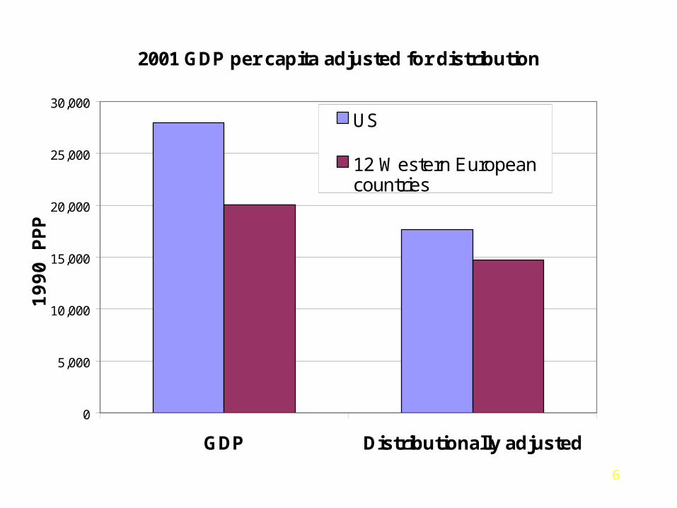
2001 GDP per capita adjusted for distribution

0

5,000

10,000

15,000

20,000

25,000

30,000

GDP Distributionally adjusted

19

90

PP

P $

US

12 Western Europeancountries

7

Figure 2 Gini coefficient and relative poverty around 2000 (60% median)

0

5

10

15

20

25

30

35

40

45

50

Slova

k R

Finla

nd

Nether

lands

Slove

nia

Belgiu

m

Norway

Sweden

Czech

R

Germ

any

Austria

Roman

ia

Poland

Hungary

Taiw

an

Canad

a

Irela

ndIta

ly UKIs

rael

Estonia

USA

Russia

Mex

ico

%

Gini

Below 60% median

8

• Substantial diversity across countries

• Makes a significant difference to how view economic performance

• Broadly similar pattern for Gini and relative poverty, but important differences

• Hard to separate history/policy stance

9

1. Introduction

2. Income inequality in OECD countries today

3.What happens to inequality as we grow richer?

4. At the bottom: absolute poverty and relative exclusion?

5. At the top: changing case for progressive taxation?

6. Conclusions

10

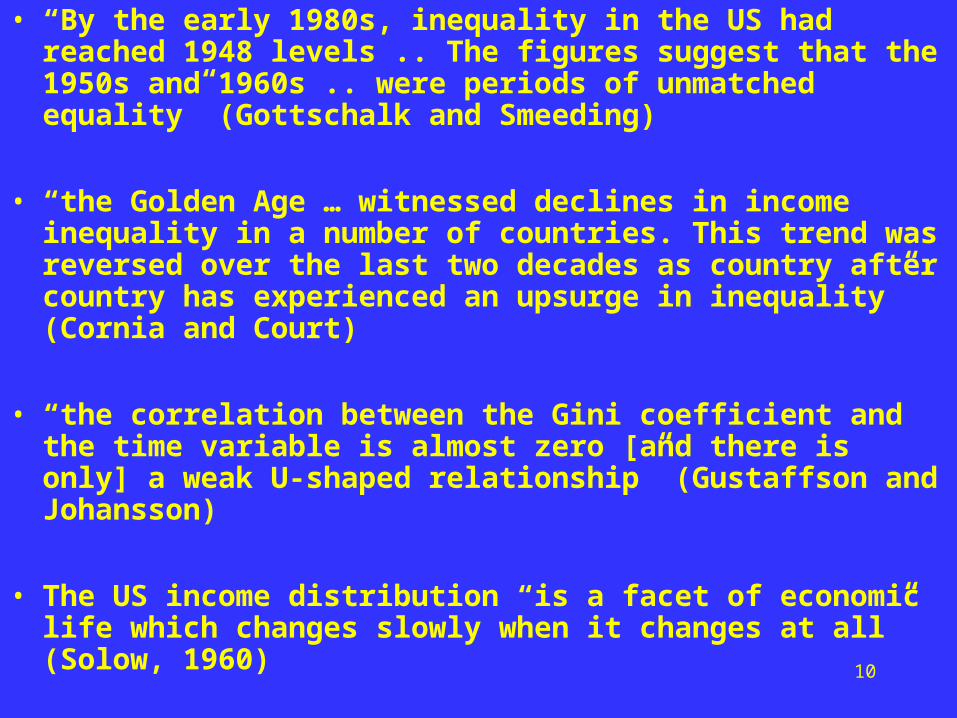
• “By the early 1980s, inequality in the US had reached 1948 levels .. The figures suggest that the 1950s and 1960s .. were periods of unmatched equality” (Gottschalk and Smeeding)

• “the Golden Age … witnessed declines in income inequality in a number of countries. This trend was reversed over the last two decades as country after country has experienced an upsurge in inequality” (Cornia and Court)

• “the correlation between the Gini coefficient and the time variable is almost zero [and there is only] a weak U-shaped relationship” (Gustaffson and Johansson)

• The US income distribution “is a facet of economic life which changes slowly when it changes at all” (Solow, 1960)

11

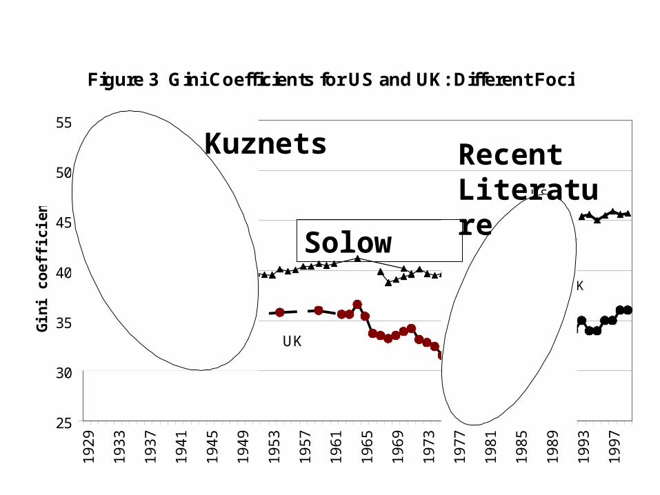
Figure 3 Gini Coefficients for US and UK: Different Foci

25

30

35

40

45

50

55

1929

1933

1937

1941

1945

1949

1953

1957

1961

1965

1969

1973

1977

1981

1985

1989

1993

1997

Gin

i co

effi

cien

t %

US

UK

UK

US

Solow

Kuznets Recent Literature

12

?

or

13

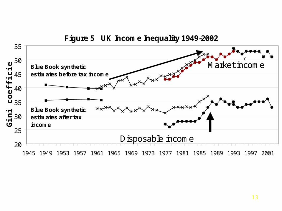
Figure 5 UK Income Inequality 1949-2002

20

25

30

35

40

45

50

55

1945 1949 1953 1957 1961 1965 1969 1973 1977 1981 1985 1989 1993 1997 2001

Gin

i c

oe

ffic

ien

t % Blue Book synthetic

estimates before tax income

Blue Book synthetic estimates after tax income

Market income

Disposable income

G

14

• Kuznets effect expired as he wrote in US; later in other countries

• Limited evidence of U-turn, more episodic

• Policy impact

15

1. Introduction

2. Income inequality in OECD countries today

3. What happens to inequality as we grow richer?

4.At the bottom: absolute poverty and relative exclusion?

5. At the top: changing case for progressive taxation?

6. Conclusions

16

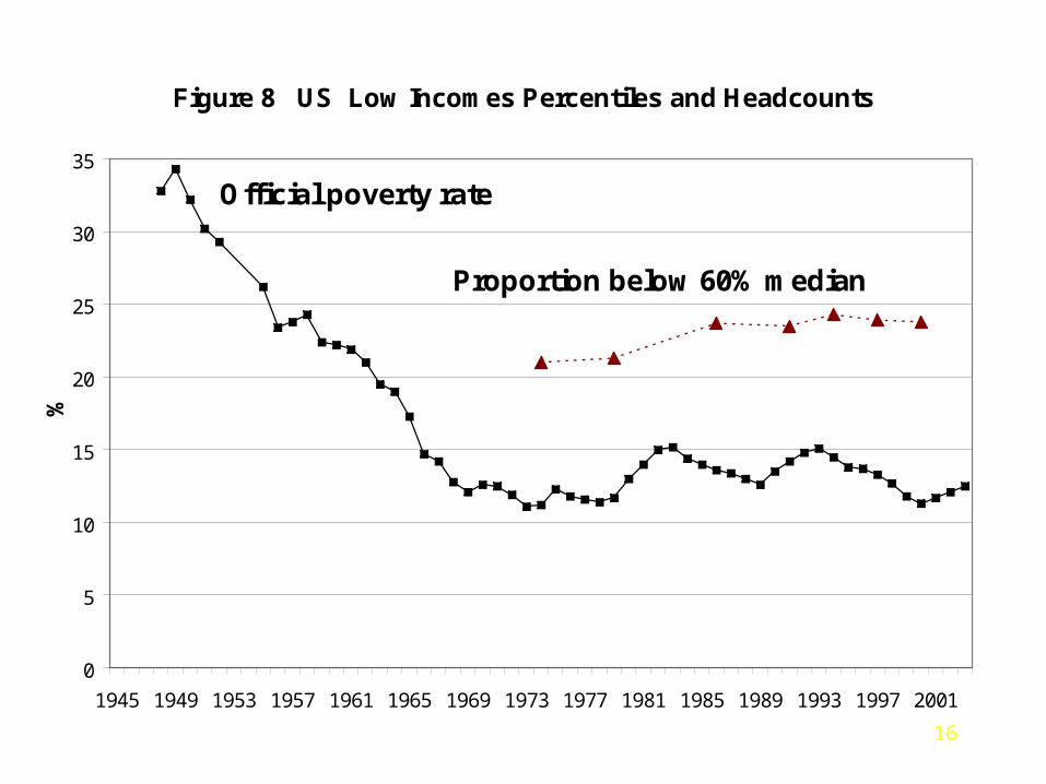
Figure 8 US Low Incomes Percentiles and Headcounts

0

5

10

15

20

25

30

35

1945 1949 1953 1957 1961 1965 1969 1973 1977 1981 1985 1989 1993 1997 2001

%

Official poverty rate

Proportion below 60% median

17

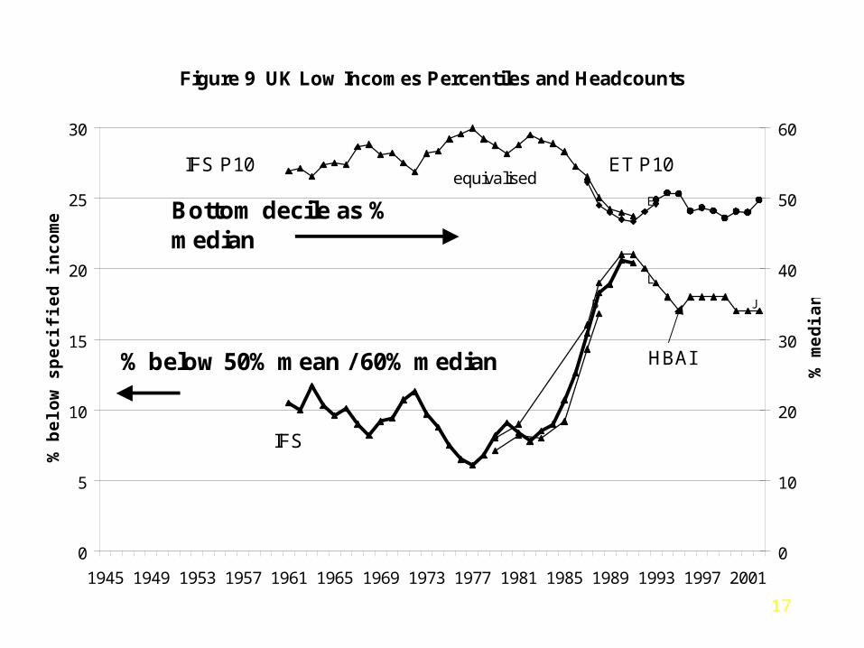
Figure 9 UK Low Incomes Percentiles and Headcounts

0

5

10

15

20

25

30

1945 1949 1953 1957 1961 1965 1969 1973 1977 1981 1985 1989 1993 1997 2001

% b

elo

w s

pe

cif

ied

in

co

me

le

ve

l

0

10

20

30

40

50

60

% m

ed

ian

IFS P10 ET P10

% below 50% mean / 60% median

IFS

HBAI

equivalised

L

E

B J

Bottom decile as % median

18

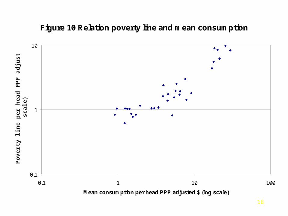
Figure 10 Relation poverty line and mean consumption

0.1

1

10

0.1 1 10 100

Mean consumption per head PPP adjusted $ (log scale)

Po

ve

rty

lin

e p

er

he

ad

PP

P a

dju

ste

d $

(lo

g

sc

ale

)

19

Figure 10(2) Relation poverty line and mean consumption

0.1

1

10

0.1 1 10 100

Mean consumption per head PPP adjusted $ (log scale)

Po

ve

rty

lin

e p

er

he

ad

PP

P a

dju

ste

d $

(lo

g

sc

ale

)

Max ($1 or 37% mean)

$2.70 a day

20

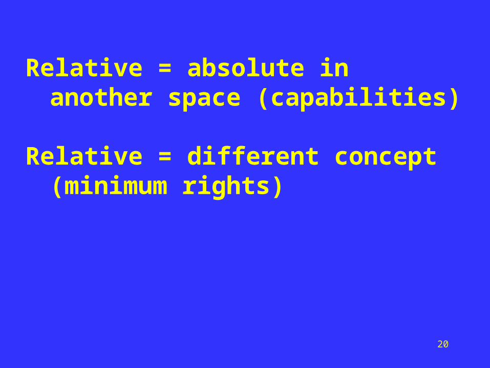
Relative = absolute in another space (capabilities)

Relative = different concept (minimum rights)

21

1. Introduction

2. Income inequality in OECD countries today

3. What happens to inequality as we grow richer?

4. At the bottom: absolute poverty and relative exclusion?

5.At the top: changing case for progressive taxation?

6. Conclusions

22

Figure 8 Shares of top income groups in total gross income in UK

02

46

810

1214

1618

20

1908 1918 1928 1938 1948 1958 1968 1978 1988 1998

% s

ha

re o

f to

tal g

ross

inco

me

02

46

810

1214

1618

20

Top 0.5%

Top 1%

Top 0.1%

23

Figure 8 Shares of top income groups in total gross income in UK 1913-2000

02468

101214161820

1908 1918 1928 1938 1948 1958 1968 1978 1988 1998

% s

hare

of

tota

l gro

ss in

com

e

02468101214161820

Top 0.5%

Top 1%

Top 0.1%

Break

24

Figure 4 Top tax rate on investment income in the UK

0

10

20

30

40

50

60

70

80

90

100

1900 1910 1920 1930 1940 1950 1960 1970 1980 1990 2000

Tax

ra

te %

X

25

Three elements relevant to choice of top tax rates:

• Elasticity of labour supply

• Distribution of earnings differences

• Social marginal valuation of income

More elastic at top?

Upper tail more extended

Changing values?

26

At low income:Priority to those in absolute poverty,

Uniformly low valuation of income above poverty line (zero in Rawlsian case)

Tax middle and top at same marginal rate

At high income:Concern with those in relative poverty,

Concerned with distribution of income among those above poverty line,

Tax middle and top at different marginal rates

27

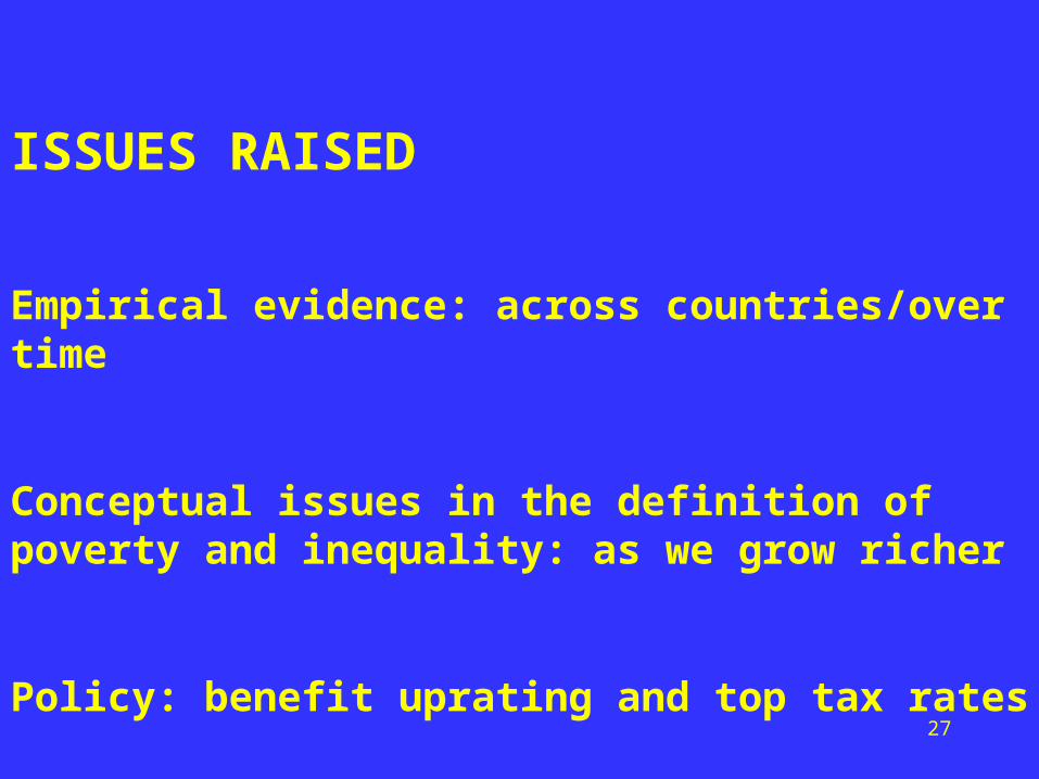
ISSUES RAISED

Empirical evidence: across countries/over time

Conceptual issues in the definition of poverty and inequality: as we grow richer

Policy: benefit uprating and top tax rates