DPRIETI Discussion Paper Series 17-E-067

Industrial Revolutions and Global Imbalances

Alexander MONGE-NARANJOFRB St. Louis / Washington University

UEDA KenichiRIETI

The Research Institute of Economy, Trade and Industryhttp://www.rieti.go.jp/en/

RIETI Discussion Paper Series17-E-067

May 2017

Industrial Revolutions and Global Imbalances*

Alexander MONGE-NARANJO (FRB St. Louis and Washington University)

UEDA Kenichi (The University of Tokyo, RIETI and TCER)

Abstract

Based on historical data since 1845, we identify a stylized fact, namely, alternating waves in global

imbalances generated by sequential industrial revolutions. We develop a new theory to explain this

stylized fact. Our theory proposes a development-stage view for the optimal global imbalances. It

explains the Lucas Paradox on capital flows as well as rises and falls in the external wealth of nations

over time.

Keywords: Global imbalance, External wealth, Industrial revolution

JEL classification: F34, F43, O19

*The views expressed in the paper are those of the authors and do not necessarily represent those of the FRB. This paper is conducted as a part of the “International Financial System and the World Economy: Medium and Long-term Issues” project undertaken at the Research Institute of Economy, Trade and Industry (RIETI). This works is also supported by JSPS Kakenhi Grant Numbers JP16K03735 and the CARF research fund at the University of Tokyo. We are grateful for helpful comments from Keiichiro Kobayashi, Makoto Yano, and participants of seminars at RIETI and the University of Tokyo. We would also like to thank for Akira Ishide, Natusmi Aizawa, and Fangyuan Yi for their excellent research assistance.

RIETI Discussion Papers Series aims at widely disseminating research results in the form of professional papers, thereby stimulating lively discussion. The views expressed in the papers are solely those of the author(s), and neither represent those of the organization to which the author(s) belong(s) nor the Research Institute of Economy, Trade and Industry.

2

I. INTRODUCTION

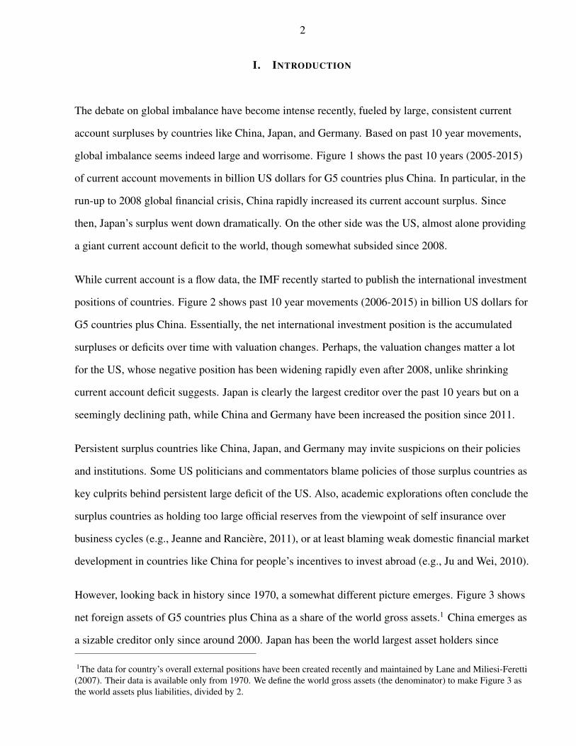
The debate on global imbalance have become intense recently, fueled by large, consistent current

account surpluses by countries like China, Japan, and Germany. Based on past 10 year movements,

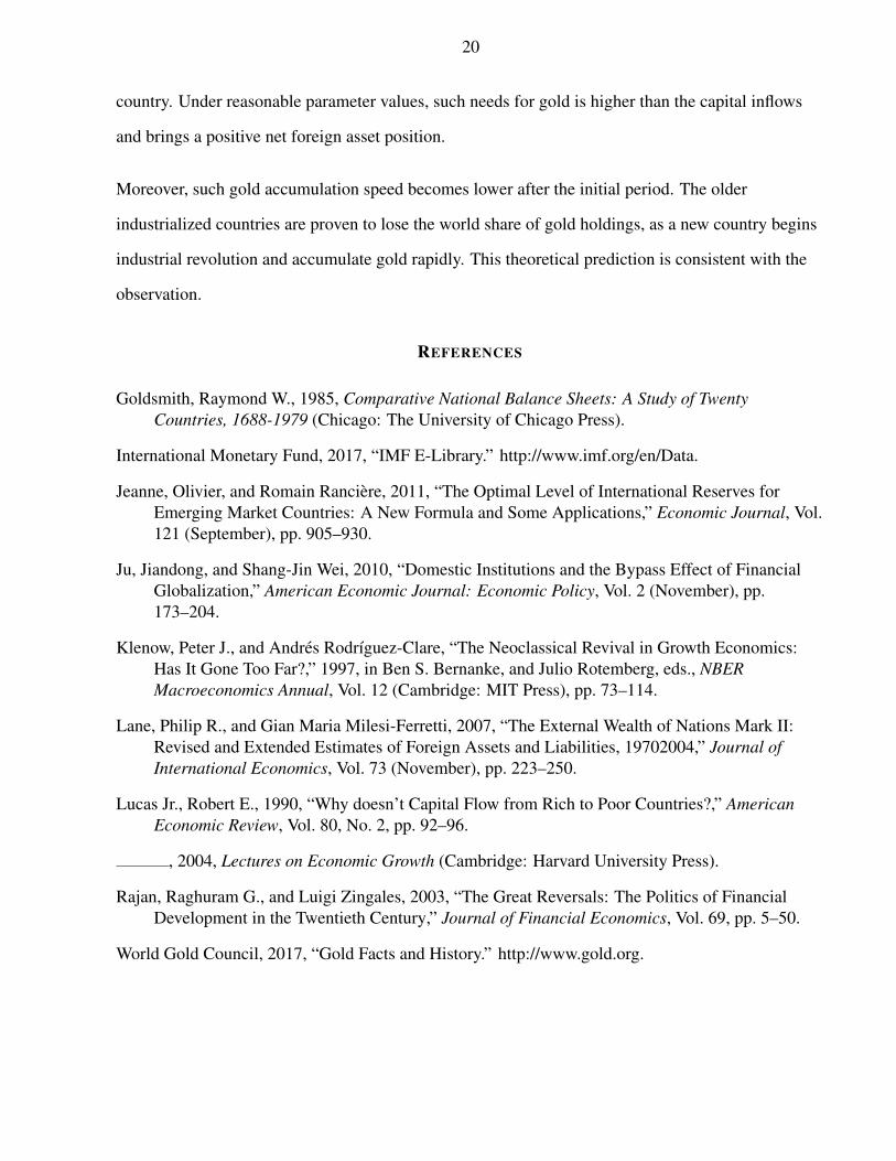
global imbalance seems indeed large and worrisome. Figure 1 shows the past 10 years (2005-2015)

of current account movements in billion US dollars for G5 countries plus China. In particular, in the

run-up to 2008 global financial crisis, China rapidly increased its current account surplus. Since

then, Japan’s surplus went down dramatically. On the other side was the US, almost alone providing

a giant current account deficit to the world, though somewhat subsided since 2008.

While current account is a flow data, the IMF recently started to publish the international investment

positions of countries. Figure 2 shows past 10 year movements (2006-2015) in billion US dollars for

G5 countries plus China. Essentially, the net international investment position is the accumulated

surpluses or deficits over time with valuation changes. Perhaps, the valuation changes matter a lot

for the US, whose negative position has been widening rapidly even after 2008, unlike shrinking

current account deficit suggests. Japan is clearly the largest creditor over the past 10 years but on a

seemingly declining path, while China and Germany have been increased the position since 2011.

Persistent surplus countries like China, Japan, and Germany may invite suspicions on their policies

and institutions. Some US politicians and commentators blame policies of those surplus countries as

key culprits behind persistent large deficit of the US. Also, academic explorations often conclude the

surplus countries as holding too large official reserves from the viewpoint of self insurance over

business cycles (e.g., Jeanne and Ranciere, 2011), or at least blaming weak domestic financial market

development in countries like China for people’s incentives to invest abroad (e.g., Ju and Wei, 2010).

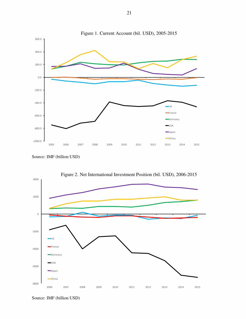
However, looking back in history since 1970, a somewhat different picture emerges. Figure 3 shows

net foreign assets of G5 countries plus China as a share of the world gross assets.1 China emerges as

a sizable creditor only since around 2000. Japan has been the world largest asset holders since

1The data for country’s overall external positions have been created recently and maintained by Lane and Miliesi-Feretti(2007). Their data is available only from 1970. We define the world gross assets (the denominator) to make Figure 3 asthe world assets plus liabilities, divided by 2.

3

mid-1980s though its relative significance lowered from 2000 along with China’s emergence. Before

1990, however, Germany and the U.K were more important creditors of the world. But, by far the

largest asset holder at least before 1980 was the US. Although its significance eroded since 1970, the

US is the main source of global imbalance as the dominant creditor for many years. Indeed, the

picture is omitted but the US played such a dominant role among the world creditors from the end of

the World War II to around 1970.

The US as the giant creditor of the world after 1945 until 1980 could be perhaps viewed as just a

unique non-economic event due to the World War II. And, if so, the global imbalance between 1845

and 1980 could be thought of as exogenous to a structural economic model. However, this view does

not seem warranted if we look back further into history before 1940. Figure 4 shows the official gold

holdings as the world share between 1845 to 1940. Note that before 1970, with the exception in

1930s, these G5 countries adopted the gold standard most of the time. Since the data for foreign

assets is scarce before 1970, we use the official gold holdings data as a proxy for the net foreign

assets. Actually, the gold is likely a good proxy for international financial assets between 1930 and

1970, because during these years the international capital markets were hardly active, worse than

1920, due to restrictive policy measures (Rajan and Zingales, 2003).

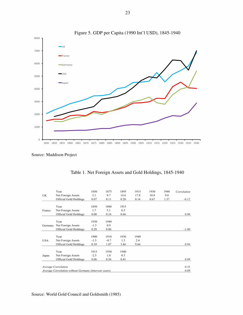
Some data before the World War II on net foreign assets is available by Goldsmith (1985). Table 1

shows that the correlation between the net foreign assets and the official gold holdings between 1850

and 1940 for G5 countries.2 Though only several years (UK) to only two years (Germany) coverage,

we compute the country specific correlations and then report the average correlation of G5 countries.

It is about 0.35. Two year coverage of Germany are 1930 and 1940, during the interwar period when

Germany’s international asset position should be regarded as exogenously determined due to World

War I reparations. So, if we take out them, the overall correlation is 0.69, implying the official gold

holdings is a good proxy for the net foreign asset position under the gold standard.

Figure 4 shows that the global imbalances, seemingly caused by newly industrialized countries, have

2We can trace figures of externally issued government bonds (i.e., liabilities) of major countries back to 19the centurybut unfortunately such data is scarce on wealth side, i.e., which countries owns those bonds. On the other hand, partlybecause of the gold standard, the official gold holdings data and price data is well available back to 19th century.

4

always existed in the world since the United Kingdom experienced the Industrial Revolution. The

UK accumulated tremendous external wealth by the mid-19th century. After the UK, France, and

Germany, though somewhat to a lesser extent, took over the UK’s position in the world after 1860.

By the beginning of the 20th century, the US then took over the status of the world largest asset

holders. Then, the US emerged in the inter-war period as the dominant external wealth holder.

A canonical pattern in these figures can be simply put as alternating large external wealth holdings

generated by sequential industrial revolutions. Each global imbalance episode is quite persistent,

nothing to do with business cycles, which however researchers often try to relate to the optimal

foreign reserve levels (e.g., Jeanne and Ranciere, 2011). Also, unlike a possible explanation for the

current Chinese economy by Ju and Wei (2010), under-development of the domestic financial market

relative to other countries cannot be a factor to explain the UK or the US as the biggest creditor of

the world for decades in the history.

Here, a new theory is needed. From the next section, we present a theoretical model that is consistent

with the identified stylized fact.

II. MODEL SETUP

There is a continuum of agents live in finitely many countries (total S countries). Countries with the

same population are distributed uniformly in [1, S], as if indexed by s with the cumulative

distribution denoted by Ω. The world total population mass is normalized to be 1, i.e., Ω(S) = 1 and

Ω(1) = 0. Production of a representative firm in country s in year t is given as

Ys,t = Kνs,t (γs,tLs,t)

1−ν , (1)

where Ks,t is capital, Ls,t is labor, and γs,t is productivity of a representative firm of country s in year

t.

Each country starts with very low level of productivity, as in pre-industrial age. However, at some

point of time, each country start to be industrialized. Here, t = 0, 1, 2, · · · indicate the calendar time

5

and s indicate the entry year of a country into industrial, modern growth. In other words, the country

indexed by s is the country that starts industrialization from year s. Country s = 1 is the “frontier”

country, which is industrialized at time 1. All countries s = 1, 2, 3, · · · have a chance of

industrialization with probability ρ in every year until they begin industrialization. In other words,

mass ρ of people, as citizens of a country, starts industrialization every year.

For a country that is not yet industrialized, productivity stays at the lowerbound, pre-industrial level,

i.e., for t < s,

γs,t = γ. (2)

The productivity of the frontier country is assumed to follow a simple Solow-type exogenous

growth, with growth rate α,

γ1,t = (1 + α)γ1,t−1 = (1 + α)tγ. (3)

Following Lucas (2004), the productivity of any follower country s ≥ 2 in t is assumed to catch up

to that of the frontier country in each year gradually, i.e., for t ≥ s3

γs,t = (1 + α)γθ1,tγ1−θs,t−1. (4)

Firms are set up and shut down each year. We assume that capital is freely mobile across countries

but that labor cannot move out of country borders. The capital and labor are owned by households,

who work for local firms but lend capital to firms anywhere in the world. The real rental price of

capital is given by rt, the same for all countries but varies over years, and the real wage is given by

ws,t for each country in each year.

A country s’s representative firm’s problem is, for each year,

maxKs,t,Ls,t

Kνs,t (γs,tLs,t)

1−ν − rtKs,t − ws,tLs,t. (5)

3The formula below is a bit simpler than Lucas (2004).

6

A representative household in each country maximizes their discounted sum of utilities over time.

For each country, the initial endowment of gold in ton is denoted as Ms,0 and capital in real term ks,0.

Also, one unit of time to work ls,t is endowed in each period for a representative household in each

country. There is no disutility from working. Income of a representative household consists of labor

income ws,tls,t and capital income rtks,t.

At the beginning of each period, households start working for and lend capital to firms. In the middle

of each period, firms produce outputs. At the end of each period, firms deliver their outputs as

consumption cs,t and investments is,t, and next-period gold Ms,t+1 (as investment), to households in

exchange for payments.

We assume that consumption goods cs,t are cash goods, required to be paid by gold Ms,t (i.e., the

gold-in-advance constraint). On the other hand, households are assumed to be able to use credits to

pay for investment goods is,t and next-period gold Ms,t+1 (i.e., credit goods). Firms use the credits

from sales to pay wages and capital rents to households and settle the credits and the debits with the

households by the end of each period.

Apparently, the financial system is incomplete. Consumption goods can be transacted only with

gold, while investments can be settled by within-period credits, presumably because creditors can

seize capital and gold easily. The capital stock can be lent or borrowed also with within-period rental

contracts, though leases, loans, or equity contracts are indistinguishable in this model. What is not

assumed available is the market for contingent claims, contingent on all countries’ starting years of

industrialization, which is the only source of risk in this model. Gold is then accumulated as a

vehicle for self insurance against industrialization status of the world.

In summary, a country s’s representative household’s problem after starting industrialization depends

on year s, when they start industrialization, and gold and capital stocks as state variables. It can be

written recursively for a representative household living in country s, for t ≥ s with u(·) denoting

the period utility,

Vs(Ms, ks) = maxM ′s,k

′s

u(cs) + βVs(M′s, k′s), (6)

7

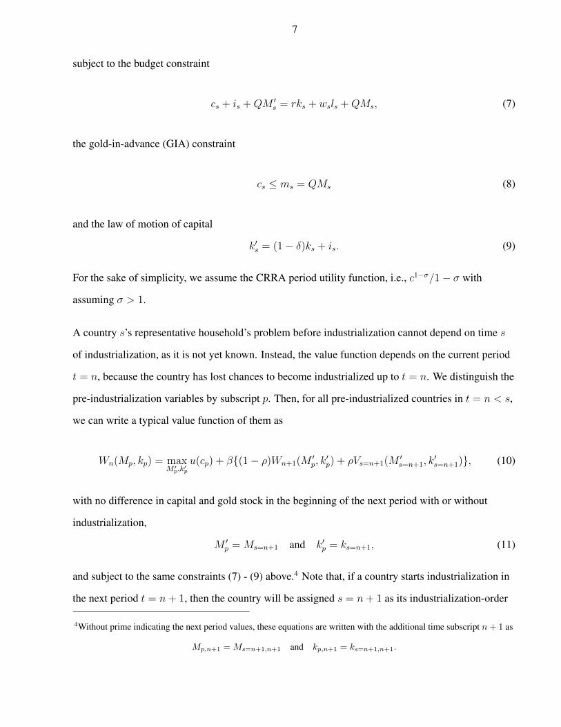
subject to the budget constraint

cs + is +QM ′s = rks + wsls +QMs, (7)

the gold-in-advance (GIA) constraint

cs ≤ ms = QMs (8)

and the law of motion of capital

k′s = (1− δ)ks + is. (9)

For the sake of simplicity, we assume the CRRA period utility function, i.e., c1−σ/1− σ with

assuming σ > 1.

A country s’s representative household’s problem before industrialization cannot depend on time s

of industrialization, as it is not yet known. Instead, the value function depends on the current period

t = n, because the country has lost chances to become industrialized up to t = n. We distinguish the

pre-industrialization variables by subscript p. Then, for all pre-industrialized countries in t = n < s,

we can write a typical value function of them as

Wn(Mp, kp) = maxM ′p,k

′p

u(cp) + β(1− ρ)Wn+1(M′p, k′p) + ρVs=n+1(M

′s=n+1, k

′s=n+1), (10)

with no difference in capital and gold stock in the beginning of the next period with or without

industrialization,

M ′p = Ms=n+1 and k′p = ks=n+1, (11)

and subject to the same constraints (7) - (9) above.4 Note that, if a country starts industrialization in

the next period t = n+ 1, then the country will be assigned s = n+ 1 as its industrialization-order

4Without prime indicating the next period values, these equations are written with the additional time subscript n+ 1 as

Mp,n+1 = Ms=n+1,n+1 and kp,n+1 = ks=n+1,n+1.

8

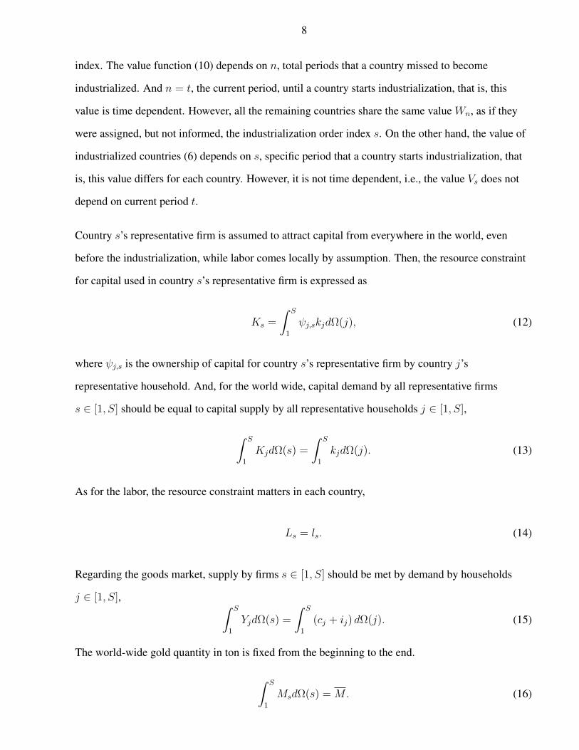
index. The value function (10) depends on n, total periods that a country missed to become

industrialized. And n = t, the current period, until a country starts industrialization, that is, this

value is time dependent. However, all the remaining countries share the same value Wn, as if they

were assigned, but not informed, the industrialization order index s. On the other hand, the value of

industrialized countries (6) depends on s, specific period that a country starts industrialization, that

is, this value differs for each country. However, it is not time dependent, i.e., the value Vs does not

depend on current period t.

Country s’s representative firm is assumed to attract capital from everywhere in the world, even

before the industrialization, while labor comes locally by assumption. Then, the resource constraint

for capital used in country s’s representative firm is expressed as

Ks =

∫ S

1

ψj,skjdΩ(j), (12)

where ψj,s is the ownership of capital for country s’s representative firm by country j’s

representative household. And, for the world wide, capital demand by all representative firms

s ∈ [1, S] should be equal to capital supply by all representative households j ∈ [1, S],

∫ S

1

KjdΩ(s) =

∫ S

1

kjdΩ(j). (13)

As for the labor, the resource constraint matters in each country,

Ls = ls. (14)

Regarding the goods market, supply by firms s ∈ [1, S] should be met by demand by households

j ∈ [1, S], ∫ S

1

YjdΩ(s) =

∫ S

1

(cj + ij) dΩ(j). (15)

The world-wide gold quantity in ton is fixed from the beginning to the end.

∫ S

1

MsdΩ(s) = M. (16)

9

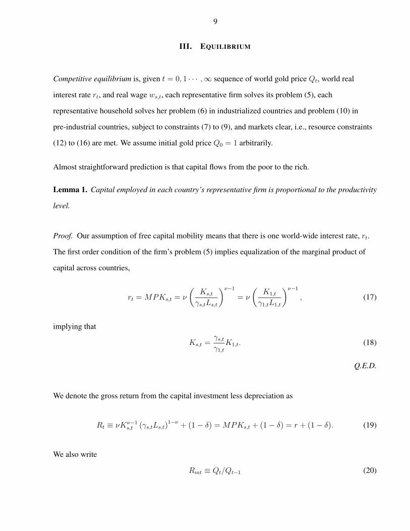
III. EQUILIBRIUM

Competitive equilibrium is, given t = 0, 1 · · · ,∞ sequence of world gold price Qt, world real

interest rate rt, and real wage ws,t, each representative firm solves its problem (5), each

representative household solves her problem (6) in industrialized countries and problem (10) in

pre-industrial countries, subject to constraints (7) to (9), and markets clear, i.e., resource constraints

(12) to (16) are met. We assume initial gold price Q0 = 1 arbitrarily.

Almost straightforward prediction is that capital flows from the poor to the rich.

Lemma 1. Capital employed in each country’s representative firm is proportional to the productivity

level.

Proof. Our assumption of free capital mobility means that there is one world-wide interest rate, rt.

The first order condition of the firm’s problem (5) implies equalization of the marginal product of

capital across countries,

rt = MPKs,t = ν

(Ks,t

γs,tLs,t

)ν−1= ν

(K1,t

γ1,tL1,t

)ν−1, (17)

implying that

Ks,t =γs,tγ1,t

K1,t. (18)

Q.E.D.

We denote the gross return from the capital investment less depreciation as

Rt ≡ νKν−1s,t (γs,tLs,t)

1−ν + (1− δ) = MPKs,t + (1− δ) = r + (1− δ). (19)

We also write

Rmt ≡ Qt/Qt−1 (20)

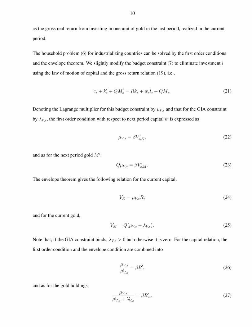
10

as the gross real return from investing in one unit of gold in the last period, realized in the current

period.

The household problem (6) for industrializing countries can be solved by the first order conditions

and the envelope theorem. We slightly modify the budget constraint (7) to eliminate investment i

using the law of motion of capital and the gross return relation (19), i.e.,

cs + k′s +QM ′s = Rks + wsls +QMs. (21)

Denoting the Lagrange multiplier for this budget constraint by µV,s and that for the GIA constraint

by λV,s, the first order condition with respect to next period capital k′ is expressed as

µV,s = βV ′s,K , (22)

and as for the next period gold M ′,

QµV,s = βV ′s,M . (23)

The envelope theorem gives the following relation for the current capital,

VK = µV,sR, (24)

and for the current gold,

VM = Q(µV,s + λV,s). (25)

Note that, if the GIA constraint binds, λV,s > 0 but otherwise it is zero. For the capital relation, the

first order condition and the envelope condition are combined into

µV,sµ′V,s

= βR′, (26)

and as for the gold holdings,µV,s

µ′V,s + λ′V,s= βR′m. (27)

11

This implies that, when deciding investment on next period gold, the next period GIA constraint

matters.

The first order condition with respect to consumption is, if constrained by the GIA,

u′(cs) = µV,s + λV,s. (28)

Hence, the Euler equation regarding capital becomes,

u′(cs)− λV,su′(c′s)− λ′V,s

= βR′. (29)

The Euler equation regarding gold can be also written as,

u′(cs)− λV,su′(c′s)

= βR′m < βR′. (30)

Next, we solve for the household problem of pre-modern economy (10). In period t = n, we assign

the Lagrange multiplier µW,n for the budget constraint and λW,n for the GIA constraint. But, as

usual, subscript n is omitted as much as possible below. Their envelope conditions and the first order

condition for consumption are essentially identical to those of the industrialized countries. However,

the first order conditions with respect to the next-period capital k′ becomes slightly different,

µW = β(1− ρ)W ′K + ρV ′s=n+1,K, (31)

and that for the next-period gold M ′, if constrained, becomes

QµW = β(1− ρ)W ′M + ρV ′s=n+1,M. (32)

Together with the envelop conditions,

µW(1− ρ)µ′W + ρµ′V,s=n+1

= βR′, (33)

12

and for the gold holdings

µW

(1− ρ) (µ′W + λ′W ) + ρ(µ′V,s=n+1 + λ′V,s=n+1

) = βR′m. (34)

Using the first order condition for consumption, similar to (28), we substitute µ and λ by the

marginal utilities. Note that, for a unconstrained country, µ′W denotes the next-period marginal utility

of consumption when this country stays in the pre-modern economy, while µ′V,s=n+1 denotes the

next-period marginal utility of consumption when this country starts industrialization in the next

period, n+ 1. Therefore, weighted average of them with ρ probability weights can be expressed as

the expected marginal utility, E[u(c′)]. However, in the next period, consumption of countries at the

pre-modern stage in the current period will be identical because it is constrained by the same value

of gold holdings Q′M ′. Thus, this is no need to use expectation operation for the next-period utility.

Then, the Euler equation can be expressed as

u′(cp)− λWu′(c′p)− E[λ′n]

= βR′, (35)

where E[λ′] = (1− ρ)λ′W + ρλ′V,s=n+1, and for the gold holdings,

u′(cp)− λWu′(c′p)

= βR′m < βR′. (36)

IV. PERIOD 0: PRE-MODERN WORLD

Assumption 1. At t = 0, when no country is industrialized yet, every country is assumed to be

identical and in the steady state expecting probability ρ of starting industrialization next period.

Assumption 1 simplifies the analysis of the pre-modern world focusing on the steady state. Because

every country knows they would be industrialized with small chances from the next period on, this

pre-modern steady state can be considered as a dawn of industrialization. As assumed, the initial

gold price is Q0 = 1, and moreover, we assume here that period zero is steady state, as if the world

13

would stay in period 0 for a long run. These assumptions automatically pin down the return on gold

in period 0 as Rm = 1 < R because the gold price is stable at 1. Hence, no country would like to

hold gold more than needed to purchase consumption goods. In other words, consumption is just

constrained by the gold holdings.5

V. PERIOD 1: INDUSTRIALIZATION BY THE FIRST COUNTRY

Lemma 2. In period 1, the shadow price of the current GIA constraint of the first country should be

greater than the other countries, λV,1 > λW,1.

The proof is obvious and omitted. The first country wants to consume more than other countries in

the first period, if it were not for the GIA constraint, to smooth consumption over time (i.e., the

permanent income hypothesis). This immediately implies that the shadow price of the GIA

constraint for the first country is higher than that for the other countries. However, the next period

shadow price λ′ can be chosen optimally.

Proposition 1. In period 1, with probability ρ of industrialization, the first industrializing country

attracts capital and buys gold from the rest of the world. Consumption of the first country is higher

than the other countries that remains at the pre-modern stage.

Proof. That the first country attracts capital is straightforward from Lemma 1. The question is why

the first country buys gold from the rest of the world in period 1.

Note that the consumption in period 1 is the same for all the countries, including the first country,

c1 = cp. (37)

5We could think of another pre-modern steady state, in which every country would not expect industrialization happensin future. If this were the case, however, there would be a jump in consumption and other endogenous variables, for evenyet-industrialized countries, when suddenly industrialization probability becomes positive. And, we do not consider thiscase.

14

This is because all the countries are constrained by the same gold holdings, which were already

determined in the previous period (i.e., period 0). However, the Euler equations regarding gold

holdings (30) and (36) means the equality of stochastic discount factors of all the countries,

u′(c1)− λV,1u′(c′1)

=u′(cp)− λW

u′(c′p)= βR′m. (38)

The same current consumption level with higher shadow price for the first country (Lemma 2)

implies lower next period marginal utility for the first country, u′(c′1) < u′(c′p), that is, higher

consumption for the first country

c′1 > c′p. (39)

Combining (37) and (39), the consumption growth of the first country is also higher the other

countries in period 1.

Because of the GIA constraint, the investment in next-period gold should match with the next-period

consumption,

M ′1 > M ′

p. (40)

In other words, the first country buys gold from others by the end of the first period to achieve higher

consumption in the next period. Q.E.D.

Corollary 1. The gold price goes up in period 1.

Proof. The supply of the gold is fixed at M and the demand for the gold is the world-wide

consumption. Thus the market clear condition for the gold (16) implies the equality between the

world consumption and the value of gold in each period,

C ≡∫ S

1

cjdΩ(j) = QM (41)

This immediately implies that the world consumption growth equals to the return on gold,

gc ≡C′

C=Q′

Q= R′m. (42)

15

Defining the gross growth rate of consumption as gc ≡ c′/c, we can rewrite the Euler equations (30)

and (36) as

gσc,1 −λV,1u′(c′1)

= gσc,p −λWu′(c′p)

= βR′m (43)

By substituting Rm in (43) by gc and summing up over the world, we obtain the relationship between

the world consumption growth rate as the average of each country’s consumption growth rate, which

possibly varies due to the GIA constraint,

gc =

∫ S

1

gc,jdΩ(j). =

∫ S

1

(βR′m +

λiu′(c′j)

) 1σ

dΩ(j). (44)

Overall, we have four unknowns, i.e., next period consumption c′1 and c′p and the current period

Lagrange multipliers for the GIA constraints, λV,1 and λW . But, we can identify them as we have

also four equations, i.e., two Euler equations in (43), definition of world consumption growth rate

(42), and the world consumption growth rate represented by an average of each country’s

consumption growth rate (44).

Importantly, the return on gold becomes higher Rm > 1 in period 1 because of the positive

consumption growth of the first country in (42). Given our initial price assumption Q0 = 1, this

means Q1 = Rm,1 > 1. That is, the gold price goes up in period 1. Q.E.D.

Corollary 2. The expected shadow price of the next period GIA constraint is smaller for the first

country than those for the other countries, i.e., λ′V,1 < E[λ′1].

Proof. The Euler equations regarding capital investments (29) and (35) means

u′(c1)− λV,1u′(c′1)− λ′V,1

=u′(cp)− λWu′(c′p)− E[λ′1]

= βR′. (45)

Comparing the above equation with (38), and using (39), it must be the case that

λ′V,1E[λ′1]

=u′(c′1)

u′(c′p)< 1. (46)

16

Q.E.D.

Claim. Not only accumulating gold, the first country has a positive net foreign asset position under

reasonable parameter values.

The capital flows into the first country (Lemma 1). Then, the net foreign asset position is equal to the

gold holdings minus capital inflow in our model. The capital inflow is roughly about the difference

between the capital of a pre-modern country and the capital of the first country, which in period 1 is,

using equation (18),

K1 −Kp =

(γ1γ− 1

)Kp. (47)

As for the gold accumulation in value by country 1,

Q1M′1 −Q1M1 =

c′1R′m− c1 =

(g′c1R′m− 1

)c1 =

(g′c1g′c− 1

)c1. (48)

where the last equation is implied by equation (42). Here, the question is whether the capital inflow

is less than the gold accumulation, i.e., in terms of per capita GDP,

(γ1γ− 1

)Kp,1

Y1,1<

(g′c1g′c− 1

)c1,1Y1,1

. (49)

Because the output growth of the first country is higher than the capital growth of a pre-modern

country, Kp,1/Y1,1 < Kp,0/Yp,0. In the modern US, presumably around the steady state, the capital to

output ratio is known to be about 2, but in the pre-modern world, it can be much smaller, even

smaller than one (see e.g., Klenow and Rodrıguez-Clare, 1997). On the other hand, consumption to

output ratio c1,1/Y1,1 can be also near one, especially for poor countries where many people live hand

to mouth. In the modern US, it is known to be around 0.95. Then, inequality (49) is likely to hold if

g′c1g′c

>γ1γ. (50)

This is probably satisfied. The left hand side is the consumption growth difference of the first

country relative to the world average growth from period 1 to 2, while the right hand side is the TFP

17

difference between the industrializing country and the pre-modern countries in period 1. Under the

closed economy assumption they should be about the same, but under our open economy

assumption, the consumption growth jumps in the period of starting industrialization.

Indeed, we can argue more clearly. In the left hand side of (50), the growth differential is equal to the

next-period consumption difference given the same current consumption due to the GIA constraint.

And, the TFP ratio in the right hand side is equal to the output ratio. Hence, inequality (50) can be

rewritten as the relation in the next period (i.e., period 2),

c1,2c2

>Y1,2

Y 2

. (51)

Noting that the average consumption and output are approximately the same as those of the

pre-modern countries, this becomesc1,2Y1,2

>cp,2Yp,2

. (52)

This relation in the next period should be satisfied because the permanent income hypothesis implies

a larger propensity to consume in a country with a higher income growth trend.6

VI. PERIOD 2: INDUSTRIALIZATION BY THE SECOND COUNTRY

The comparative analysis between the second country and s ≥ 3 countries in period 2 is almost

identical to what described in Proposition 1 for the first country and the other countries. Hence, we

focus the relation between the first country and the second country here.

Proposition 2. The growth of consumption, and gold holdings, by the second country are higher

than those of the first country from period 2 to 3.

Proof. In period 2, Corollary 2 suggests that λV,1 ≤ E[λ′1] is determined already in teh previous

period (i.e., period1). However, Lemma 2 should also apply to period 2 for the second country and

6We do not assume wealth effects of consumption as we use the CRRA period-utility function. Note that, in the firstperiod when a country starts industrialization, the first country limits consumption due to the severe GIA constraint, butfrom the next period on, the first country can choose the gold optimally to mitigate the severity of the GIA constraint(Corollary 2).

18

s ≥ 3 countries and thus λV,2 > λW . Because E[λ′1] is the weighted average of λV,2 and λW,2,

λV,1 < λV,2. (53)

In period 2, the first country and the second country share the same Euler equation (30) as

industrializing countries,

.u′(c1)− λV,1

u′(c′1)=u′(c2)− λV,2

u′(c′2), (54)

implying that

.u′(c′2)

u′(c′1)=u′(c2)− λV,2u′(c1)− λV,1

<u′(c2)

u′(c1), (55)

where the last inequality comes from (53). Divide the right hand side by the left hand side, and obtain

.1 >

u′(c′2)

u′(c′1)

u′(c2)u′(c1)

=gσc,1gσc,2

, (56)

that is,

gc,1 < gc,2. (57)

As their consumption both constrained by the value of gold holdings QMs, it must be also the case

that the growth rate of gold holdings by the second country must be higher than that of the first

country, i.e.,M ′

1

M1

<M ′

2

M2

(58)

Q.E.D.

Note that, although the growth of consumption (and gold holdings) is higher in country 2 than in

country 1, the level of consumption (and gold holding) is not necessarily higher in country 2 than

country 1. Rather, the consumption level country 2 catches up to that of country 1 from below. Still,

apparently, the world share of consumption (and gold holdings) of country 2 increases as the share of

country 1 declines.

19

Period 3 and later can be characterized as the similar way as for period 2: a new taking-off country

grows most rapidly and accumulates international assets most quickly.

VII. CONCLUSION

We have identified a stylized fact, that is, alternating waves in historical global imbalance generated

by sequential industrial revolutions. Newly industrialized countries often accumulate foreign assets

as they grow rapidly. This pattern occurs several times since at least mid-19th century.

We propose a new theoretical model to explain this stylized fact by applying the sequential industrial

revolution model of Lucas (2004) to an open economy setup, combined with the hard currency

(gold) constraint to buy consumption goods. In the period when a country takes off, the country

faces the severe gold constraint to limit consumption. As the country becomes sure about receiving a

higher income, it saves and invests more rapidly than the others including already industrialized

countries, and than the pre-industrialized days of itself.

Note that the catch-up process of the GDP and consumption in Lucas (2004) occurs solely due to the

assumed sequential TFP growth under the closed economy assumption. In this paper, we consider an

open economy, which seems more consistent with the real-world experience of industrial revolutions.

If we assumed the perfect markets, contingent claims can insure all the risks, including the timings

of industrial revolutions, at time zero. Such perfect insurance would mean that the consumption over

time would be the same for all ex ante identical countries. The capital still flows to the higher TFP

countries (i.e., the Poor to the Rich, the Lucas Paradox (Lucas, 1990)) to equate the marginal product

of capital among countries. Then, without additional international assets, the net foreign asset

positions are negative for earlier industrializing countries, inconsistent with the stylized facts.

On the contrary, in this paper, we assume an incomplete market to insure against timings of

industrial revolutions and the hard currency constraint for consumption goods purchase. These

international finance frictions create strong needs for the hard currency by a newly industrializing

20

country. Under reasonable parameter values, such needs for gold is higher than the capital inflows

and brings a positive net foreign asset position.

Moreover, such gold accumulation speed becomes lower after the initial period. The older

industrialized countries are proven to lose the world share of gold holdings, as a new country begins

industrial revolution and accumulate gold rapidly. This theoretical prediction is consistent with the

observation.

REFERENCES

Goldsmith, Raymond W., 1985, Comparative National Balance Sheets: A Study of TwentyCountries, 1688-1979 (Chicago: The University of Chicago Press).

International Monetary Fund, 2017, “IMF E-Library.” http://www.imf.org/en/Data.

Jeanne, Olivier, and Romain Ranciere, 2011, “The Optimal Level of International Reserves forEmerging Market Countries: A New Formula and Some Applications,” Economic Journal, Vol.121 (September), pp. 905–930.

Ju, Jiandong, and Shang-Jin Wei, 2010, “Domestic Institutions and the Bypass Effect of FinancialGlobalization,” American Economic Journal: Economic Policy, Vol. 2 (November), pp.173–204.

Klenow, Peter J., and Andres Rodrıguez-Clare, “The Neoclassical Revival in Growth Economics:Has It Gone Too Far?,” 1997, in Ben S. Bernanke, and Julio Rotemberg, eds., NBERMacroeconomics Annual, Vol. 12 (Cambridge: MIT Press), pp. 73–114.

Lane, Philip R., and Gian Maria Milesi-Ferretti, 2007, “The External Wealth of Nations Mark II:Revised and Extended Estimates of Foreign Assets and Liabilities, 19702004,” Journal ofInternational Economics, Vol. 73 (November), pp. 223–250.

Lucas Jr., Robert E., 1990, “Why doesn’t Capital Flow from Rich to Poor Countries?,” AmericanEconomic Review, Vol. 80, No. 2, pp. 92–96.

, 2004, Lectures on Economic Growth (Cambridge: Harvard University Press).

Rajan, Raghuram G., and Luigi Zingales, 2003, “The Great Reversals: The Politics of FinancialDevelopment in the Twentieth Century,” Journal of Financial Economics, Vol. 69, pp. 5–50.

World Gold Council, 2017, “Gold Facts and History.” http://www.gold.org.

21

Figure 1. Current Account (bil. USD), 2005-2015

-1000.0

-800.0

-600.0

-400.0

-200.0

0.0

200.0

400.0

600.0

2005 2006 2007 2008 2009 2010 2011 2012 2013 2014 2015

UK

France

Germany

USA

Japan

China

Source: IMF (billion USD)

Figure 2. Net International Investment Position (bil. USD), 2006-2015

-8000

-6000

-4000

-2000

0

2000

4000

2006 2007 2008 2009 2010 2011 2012 2013 2014 2015

UK

France

Germany

USA

Japan

China

Source: IMF (billion USD)

22

Figure 3. Net Foreign Assets, World Share (%), 1970-2010

-0.1

-0.05

0

0.05

0.1

0.15

0.2

1970

1971

1972

1973

1974

1975

1976

1977

1978

1979

1980

1981

1982

1983

1984

1985

1986

1987

1988

1989

1990

1991

1992

1993

1994

1995

1996

1997

1998

1999

2000

2001

2002

2003

2004

2005

2006

2007

2008

2009

2010

UK

France

Germany

USA

Japan

China

Source: Updated data of Lane and Milesi-Ferretti (2007) by authors (the denominator is world assets plusliabilities, divided by 2)

Figure 4. World Gold Holdings Share (%), 1845-1940

0.0

10.0

20.0

30.0

40.0

50.0

60.0

70.0

80.0

90.0

100.0

1845 1850 1855 1860 1865 1870 1875 1880 1885 1890 1895 1900 1905 1910 1915 1920 1925 1930 1935 1940

UK

France

Germany

USA

Japan

Source: World Gold Council

23

Figure 5. GDP per Capita (1990 Int’l USD), 1845-1940

0

1000

2000

3000

4000

5000

6000

7000

8000

1845 1850 1855 1860 1865 1870 1875 1880 1885 1890 1895 1900 1905 1910 1915 1920 1925 1930 1935 1940

UK

France

Germany

USA

Japan

Source: Maddison Project

Table 1. Net Foreign Assets and Gold Holdings, 1845-1940

Year 1850 1875 1895 1915 1930 1940 CorrelationUK Net Foreign Assets 3.1 9.7 14.6 17.8 10.8 9.0

Official Gold Holdings 0.07 0.11 0.20 0.16 0.67 1.57 -0.12

Year 1850 1880 1915France Net Foreign Assets 1.7 5.1 8.5

Official Gold Holdings 0.00 0.16 0.66 0.96

Year 1930 1940Germany Net Foreign Assets -1.3 0.9

Official Gold Holdings 0.28 0.06 -1.00

Year 1900 1910 1930 1940USA Net Foreign Assets -1.5 -0.7 1.3 2.4

Official Gold Holdings 0.39 1.07 3.86 9.66 0.94

Year 1915 1930 1940Japan Net Foreign Assets -2.5 1.0 0.3

Official Gold Holdings 0.06 0.56 0.41 0.99

Average Correlation 0.35Average Correlation without Germany (interwar years) 0.69

Source: World Gold Council and Goldsmith (1985)