Induction: a formal perspective

Uwe Saint-Mont, Nordhausen University of Applied Sciences∗

December 2, 2019

Abstract. The aim of this contribution is to provide a rather general answer to Hume’sproblem. To this end, induction is treated within a straightforward formal paradigm,i.e., several connected levels of abstraction.

Within this setting, many concrete models are discussed. On the one hand, modelsfrom mathematics, statistics and information science demonstrate how induction mightsucceed. On the other hand, standard examples from philosophy highlight fundamentaldifficulties.

Thus it transpires that the difference between unbounded and bounded inductive stepsis crucial: While unbounded leaps of faith are never justified, there may well be rea-sonable bounded inductive steps.

In this endeavour, the twin concepts of information and probability prove to be in-dispensable, pinning down the crucial arguments, and, at times, reducing them tocalculations.

Essentially, a precise study of boundedness settles Goodman’s challenge. Hume’s moreprofound claim of seemingly inevitable circularity is answered by obviously non-circularhierarchical structures.

Keywords

Hume’s Problem; Induction; Inference

∗Prof. U. Saint-Mont, Fachbereich Wirtschafts- und Sozialwissenschaften, Hochschule Nordhausen,Weinberghof 4, D-99734 Nordhausen; saint-mont@hs-nordhausen.de; ORCID: 0000-0001-6801-3658.

1

Contents

1 Introduction 3

2 Hume’s problem 3

2.1 Verbal exposition . . . . . . . . . . . . . . . . . . . . . . . . . . . . . . 3

2.2 Formal treatment . . . . . . . . . . . . . . . . . . . . . . . . . . . . . . 5

3 The many faces of induction 5

3.1 Philosophy . . . . . . . . . . . . . . . . . . . . . . . . . . . . . . . . . . 5

3.2 Computer Sciences . . . . . . . . . . . . . . . . . . . . . . . . . . . . . 7

3.3 Statistics . . . . . . . . . . . . . . . . . . . . . . . . . . . . . . . . . . . 10

4 Extensions 13

4.1 The multi-tier model . . . . . . . . . . . . . . . . . . . . . . . . . . . . 13

4.2 Convergence . . . . . . . . . . . . . . . . . . . . . . . . . . . . . . . . . 14

4.3 The general inductive principle . . . . . . . . . . . . . . . . . . . . . . 14

5 Successful inductions 16

5.1 A paradigmatic large gap: Connecting finite and infinite sequences . . . 16

5.2 Coping with circularity . . . . . . . . . . . . . . . . . . . . . . . . . . . 18

5.3 Invertibility . . . . . . . . . . . . . . . . . . . . . . . . . . . . . . . . . 21

6 Goodman’s challenge 23

6.1 Boundedness is crucial . . . . . . . . . . . . . . . . . . . . . . . . . . . 24

6.2 Levels of abstraction . . . . . . . . . . . . . . . . . . . . . . . . . . . . 25

7 Summary 27

References 30

2

1 Introduction

A problem is difficult if it takes a long time to solve it; it is important if a lot of crucialresults hinge on it. In the case of induction, philosophy does not seem to have mademuch progress since Hume’s time: Induction is still the glory of science and the scandalof philosophy (Broad (1952), p. 143), or as Whitehead (1926), p. 35, put it: “The theoryof induction is the despair of philosophy - and yet all our activities are based upon it.”Since a crucial feature of science is general theories based on specific data, i.e., somekind of induction, Hume’s problem seems to be both: difficult and important.

Let us first state the issue in more detail. Traditionally, many dictionaries define induc-tive reasoning as the derivation of general principles/laws from particular/individualinstances. For example, according to the Encylopedia Britannica (2018), induction isthe “method of reasoning from a part to a whole, from particulars to generals, or fromthe individual to the universal.” However, nowadays, philosophers rather couch thequestion in ‘degrees of support.’ Given valid premises, a deductive argument preservestruth, i.e., its conclusion is also valid. An inductive argument is weaker, since suchan argument transfers true premises into some degree of support for the argument’sconclusion. The truth of the premises provides (more or less) good reason to believethe conclusion to be true.

Although these lines of approach could seem rather different, they are indeed verysimilar if not identical: Strictly deductive arguments, preserving truth, can only befound in logic and mathematics. The core of these sciences is the method of proofwhich always proceeds (in a certain sense, later described more explicitly) from themore general to the less general. Given a number of assumptions, an axiom system,say, any valid theorem has to be derived from them. That is, given the axioms, afinite number of logically sound steps imply a theorem. In this sense, a theorem isalways more specific than the whole set of axioms; its content is more restricted thanthe complete realm defined by the axioms: Euklid’s axioms define a whole geometry,whereas Phythagoras’ theorem just deals with a particular kind of triangle.

Induction fits perfectly well into this picture: Since there are always several ways togeneralize a given set of data, “there is no way that leads with necessity from thespecific to the general” (Popper). In other words, one cannot prove the move from themore specific to the less specific. A theorem that holds for rectangles need not holdfor arbitrary four-sided figures. Deduction is possible if and only if we go from generalto specific. When moving from general to specific one may thus try to strengthen anon-conclusive argument until it becomes a proof. The reverse to this is, however,impossible. Strictly non-deductive arguments, those that cannot be ‘fixed’ in principle,are those which universalise some statement.

2 Hume’s problem

2.1 Verbal exposition

Gauch (2012), pp. 168 gives a concise modern exposition of the issue and its importance:

(i) Any verdict on the legitimacy of induction must result from deductiveor inductive arguments, because those are the only kinds of reasoning.

3

(ii) A verdict on induction cannot be reached deductively. No inferencefrom the observed to the unobserved is deductive, specifically becausenothing in deductive logic can ensure that the course of nature willnot change.

(iii) A verdict cannot be reached inductively. Any appeal to the past suc-cesses of inductive logic, such as that bread has continued to be nu-tritious and that the sun has continued to rise day after day, is butworthless circular reasoning when applied to induction’s future for-tunes

Therefore, because deduction and induction are the only options, and be-cause neither can reach a verdict on induction, the conclusion follows thatthere is no rational justification for induction.

Notice that this claim goes much further than some question of validity: Of course, aninductive step is never sure (may be invalid); Hume, however, disputes that inductiveconclusions, i.e., the very method of generalizing, can be justified at all. Reichenbach(1956) forcefully pointed out why this result is so devastating: Without a rationaljustification for induction, empiricist philosophy in general and science in particular,hang in the air. However, worse still, if Hume is right, such a justification quite simplydoes not exist. If empiricist philosophers and scientists only admit empirical experiencesand rational thinking, they have to contradict themselves since, at the very beginning oftheir endeavour, they need to subscribe to a transcendental reason (i.e., an argumentneither empirical nor rational). Thus, this way to proceed is, in a very deep sense,irrational.

Consistently, Hacking (2001), p. 190, writes: “Hume’s problem is not out of date [. . .]Analytic philosophers still drive themselves up the wall (to put it mildly) when theythink about it seriously.” For Godfrey-Smith (2003), p. 39, it is “The mother of allproblems.” Moreover, quite obviously, there are two major ways to respond to Hume:

(i) Acceptance of Hume’s conclusion. This seems to have been philosophy’s main-stream reaction, at least in recent decades, resulting in fundamental doubt. Con-sequently, there is now a strong tradition questioning induction, science, theEnlightenment, and perhaps even the modern era.

(ii) Challenging Hume’s conclusion and providing a more constructive answer. Thisseems to be the typical way scientists respond to the problem. Authors withinthis tradition often concede that many particular inductive steps are justified.However, since all direct attempts to solve the riddle seem to have failed, there ishardly any general justification. Tukey (1961) is quite an exception: “Statistics isa broad field, whether or not you define it as ‘The science, the art, the philosophy,and the techniques of making inferences from the particular to the general’.”

Since the basic viewpoints are so different, it should come as no surprise that, unfor-tunately, clashes are the rule and not the exception. For example, when philosophersPopper und Miller (1983) tried to do away with induction once and for all, physicistJaynes (2003), p. 699, responded: “Written for scientists, this is like trying to prove theimpossibility of heavier-than-air flight to an assembly of professional airline pilots.”

4

2.2 Formal treatment

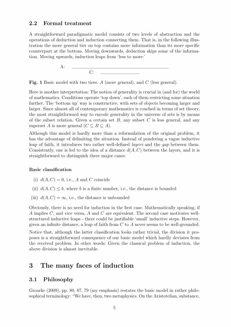
A straightforward paradigmatic model consists of two levels of abstraction and theoperations of deduction and induction connecting them. That is, in the following illus-tration the more general tier on top contains more information than its more specificcounterpart at the bottom. Moving downwards, deduction skips some of the informa-tion. Moving upwards, induction leaps from ‘less to more:’

A:C:

Fig. 1 Basic model with two tiers. A (more general), and C (less general).

Here is another interpretation: The notion of generality is crucial in (and for) the worldof mathematics. Conditions operate ‘top down’, each of them restricting some situationfurther. The ‘bottom up’ way is constructive, with sets of objects becoming larger andlarger. Since almost all of contemporary mathematics is couched in terms of set theory,the most straightforward way to encode generality in the universe of sets is by meansof the subset relation. Given a certain set B, any subset C is less general, and anysuperset A is more general (C ⊆ B ⊆ A).

Although this model is hardly more than a reformulation of the original problem, ithas the advantage of delimiting the situation. Instead of pondering a vague inductiveleap of faith, it introduces two rather well-defined layers and the gap between them.Consistently, one is led to the idea of a distance d(A,C) between the layers, and it isstraightforward to distinguish three major cases:

Basic classification

(i) d(A,C) = 0, i.e., A and C coincide

(ii) d(A,C) ≤ b, where b is a finite number, i.e., the distance is bounded

(iii) d(A,C) = ∞, i.e., the distance is unbounded

Obviously, there is no need for induction in the first case. Mathematically speaking, ifA implies C, and vice versa, A and C are equivalent. The second case motivates well-structured inductive leaps - there could be justifiable ‘small’ inductive steps. However,given an infinite distance, a leap of faith from C to A never seems to be well-grounded.

Notice that, although the latter classification looks rather trivial, the division it pro-poses is a straightforward consequence of our basic model which hardly deviates fromthe received problem. In other words: Given the classical problem of induction, theabove division is almost inevitable.

3 The many faces of induction

3.1 Philosophy

Groarke (2009), pp. 80, 87, 79 (my emphasis) restates the basic model in rather philo-sophical terminology: “We have, then, two metaphysics. On the Aristotelian, substance,

5

understood as the true nature of existence of things, is open to view. The world can beobserved. On the empiricist, it lies underneath perception; the true nature of realitylies within an invisible substratum forever closed to human penetration. . .To place sub-stance, ultimate existence, outside the limits of human cognition, is to leave us enoughmental room to doubt anything. . .It is the remoteness of this ultimate metaphysicalreality that undermines induction.”

Apart from this rather roundabout treatment, particular situations have been studiedin much detail:

Eliminative induction

A classical approach, preceding Hume, is eliminative induction. Given a number ofhypotheses on the (more) abstract layer A and a number of observations on the (more)concrete layer C, the observations help to eliminate hypotheses. In detective stories,with a finite number of suspects (hypotheses), this works fine. The same applies toan experimentum crucis that collects data in order to decide between just two rivalhypotheses.

However, the real problem seems to be unboundedness. For example, if one observationis able to delete k hypotheses, an infinite number of hypotheses will remain if there isan infinite collection of hypotheses but just a finite number of observations. That is oneof the main reasons why string theories in modern theoretical physics are notorious:On the one hand, due to their huge number of parameters, there is an abundance ofdifferent theories. On the other hand, there are hardly any (no?) observations thateffectively eliminate most of these theories (Woit 2006).

More generally speaking: If the information in the observations suffices to narrow downthe number of hypotheses to a single one, eliminative induction works. However, sincehypotheses have a surplus meaning, this could be the exception rather than the rule.

Enumerative induction

Perhaps the most prominent example of a non-convincing inductive argument is Ba-con’s enumerative induction. That is, do a finite number of observations x1, . . . , xn suf-fice to support a general law like “all swans are white”? A similar question is if/whenit is reasonable to proceed to the limit limxi = x.

Given as little as a finite sequence, the infinite limit is, of course, arbitrary. Therefore theconcept of mathematical convergence is defined the other way around: Given an infinitesequence, any finite number of elements is irrelevant (e.g., the first n). A sequence(xi)i∈IN converges towards x if ‘almost all’ xi (all except a finite set of elements) liewithin an arbitrary small neighborhood of x. That is, given some distance measured(x, y) and any ϵ > 0, then for almost all i, d(xi, x) < ϵ. This is equivalent to sayingthat for every ϵ > 0 there is an n(ϵ) such that all xi with i ≥ n do not differ more thanϵ from x, that is, for all i ≥ n we have d(xi, x) < ϵ.

Our interpretation of this situation amounts to saying that any finite sequence containsa very limited amount of information. If it is a binary sequence of length n, exactly nyes-no questions have to be answered in order to obtain a particular sequence x1, . . . , xn.In the case of an arbitrary infinite binary sequence x1, x2, x3, . . . one has to answeran infinite number of such questions. In other words, since the gap between the twosituations is not bounded, it cannot be bridged. In this situation, Hume is right when he

6

claims that “one instance is not better than none”, and that “a hundred or a thousandinstances are . . . no better than one” (cf. Stove (1986), pp. 39-40).

Further assumptions are needed, either restricting the class of infinite sequences orstrengthening the finite sequence considerably. Either way, the gap between A andC becomes smaller, and one may hope to get a reasonable result if the additionalassumptions render the distance finite. For a thorough discussion see section 5.1.

Frequentist probability

Trying to define probability in terms of a limit of empirical frequencies is a typicalexample of how not to treat the problem. Empirical observations - of course, always afinite number - may have a ‘practical limit,’ i.e., they may stabilise quickly. However,that is not a limit in the mathematical sense requiring an infinite number of (idealized)observations.1 Trying to use the empirical observation of ‘stabilisation’ as a definitionof probability (Reichenbach 1938, 1949), inevitably needs to evoke infinite sequences,a mathematical idealization.

Thus the frequentist approach easily confounds the theoretical notion of probability(a mathematical concept) with limits of observed frequencies (empirical data). In thesame vein highly precise measurements of the diameters and the perimeters of a millioncircles may give a good approximation of the number π; nevertheless, physics is notable to prove a single mathematical fact about π. Instead, mathematics must definea circle as a certain relation of ideas, and also needs to ‘toss a coin’ in a theoreticalframework. A contemporary and logically sound treatment is given in section 5.1.

3.2 Computer Sciences

Quite distinctive inductive problems can be found in this area. They range from thesmallest inductive step perceivable to malign situations:

An elementary model

The basic unit of information is the Bit. This logical unit may assume two distinctvalues (typically named 0 and 1). Either the state of the Bit B is known or set toa certain value, (e.g., B = 1), or the state of Bit B is not known or has not beendetermined, that is, B may be 0 or 1. The elegant notation used for the latter case isB =?, the question mark being called a “wildcard.”

In the first case, there is no degree of freedom: We have particular data. In the secondcase, there is exactly one (elementary) degree of freedom. Moving from the general casewith one degree of freedom to the special case with no degree of freedom is simple:Just answer the following yes-no question: “Is B equal to 1, yes or no?” Moreover,given a number of Bits, more or less general situations can be distinguished in anextraordinarily simple way: One just counts the number of yes-no questions that needto be answered (and that’s exactly what almost any introduction to information theorydoes), or, equivalently, the number of degrees of freedom lost. Thus, beside its eleganceand generality, the major advantage of this approach is the fact that everything isfinite, allowing interesting questions to be answered in a definite way.

1The essential point of the mathematical definition is the behaviour of almost all members of somesequence (i.e., all but a finite number). Therefore any number of empirical observations is not able tobridge the gap between strictly finite sequences and the realm of infinite sequences.

7

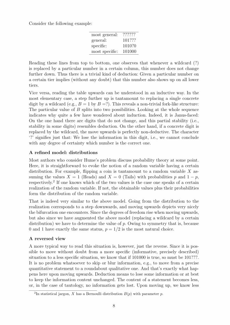
Consider the following example:

most general: ??????general: 101???specific: 1010?0most specific: 101000

Reading these lines from top to bottom, one observes that whenever a wildcard (?)is replaced by a particular number in a certain column, this number does not changefurther down. Thus there is a trivial kind of deduction: Given a particular number ona certain tier implies (without any doubt) that this number also shows up on all lowertiers.

Vice versa, reading the table upwards can be understood in an inductive way. In themost elementary case, a step further up is tantamount to replacing a single concretedigit by a wildcard (e.g., B = 1 by B =?). This reveals a non-trivial fork-like structure:The particular value of B splits into two possibilities. Looking at the whole sequenceindicates why quite a few have wondered about induction. Indeed, it is Janus-faced:On the one hand there are digits that do not change, and this partial stability (i.e.,stability in some digits) resembles deduction. On the other hand, if a concrete digit isreplaced by the wildcard, the move upwards is perfectly non-deductive. The character‘?’ signifies just that: We lose the information in this digit, i.e., we cannot concludewith any degree of certainty which number is the correct one.

A refined model: distributions

Most authors who consider Hume’s problem discuss probability theory at some point.Here, it is straightforward to evoke the notion of a random variable having a certaindistribution. For example, flipping a coin is tantamount to a random variable X as-suming the values X = 1 (Heads) and X = 0 (Tails) with probabilities p and 1 − p,respectively.2 If one knows which of the two values is the case one speaks of a certainrealization of the random variable. If not, the obtainable values plus their probabilitiesform the distribution of the random variable.

That is indeed very similar to the above model. Going from the distribution to therealization corresponds to a step downwards, and moving upwards depicts very nicelythe bifurcation one encounters. Since the degrees of freedom rise when moving upwards,but also since we have augmented the above model (replacing a wildcard by a certaindistribution) we have to determine the value of p. Owing to symmetry that is, because0 and 1 have exactly the same status, p = 1/2 is the most natural choice.

A reversed view

A more typical way to read this situation is, however, just the reverse. Since it is pos-sible to move without doubt from a more specific (informative, precisely described)situation to a less specific situation, we know that if 101000 is true, so must be 101???.It is no problem whatsoever to skip or blur information, e.g., to move from a precisequantitative statement to a roundabout qualitative one. And that’s exactly what hap-pens here upon moving upwards. Deduction means to lose some information or at bestto keep the information content unchanged. The content of a statement becomes less,or, in the case of tautology, no information gets lost. Upon moving up, we know less

2In statistical jargon, X has a Bernoulli distribution B(p) with parameter p.

8

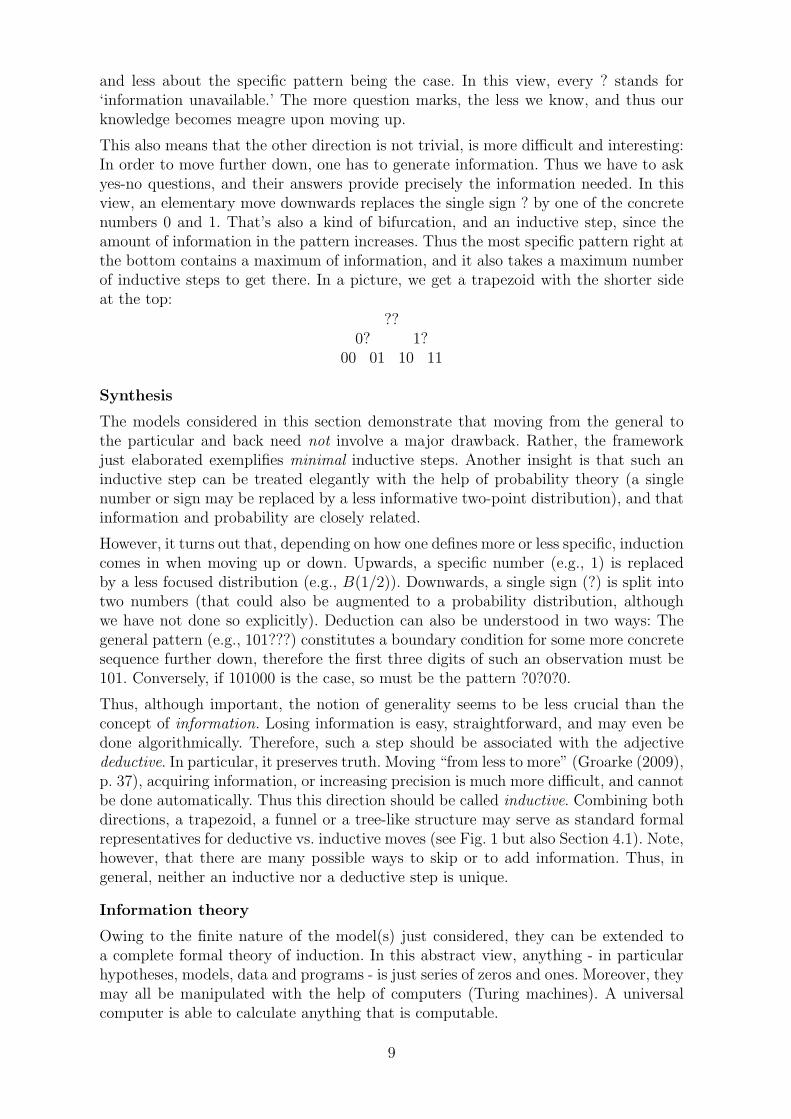
and less about the specific pattern being the case. In this view, every ? stands for‘information unavailable.’ The more question marks, the less we know, and thus ourknowledge becomes meagre upon moving up.

This also means that the other direction is not trivial, is more difficult and interesting:In order to move further down, one has to generate information. Thus we have to askyes-no questions, and their answers provide precisely the information needed. In thisview, an elementary move downwards replaces the single sign ? by one of the concretenumbers 0 and 1. That’s also a kind of bifurcation, and an inductive step, since theamount of information in the pattern increases. Thus the most specific pattern right atthe bottom contains a maximum of information, and it also takes a maximum numberof inductive steps to get there. In a picture, we get a trapezoid with the shorter sideat the top:

??0? 1?

00 01 10 11

Synthesis

The models considered in this section demonstrate that moving from the general tothe particular and back need not involve a major drawback. Rather, the frameworkjust elaborated exemplifies minimal inductive steps. Another insight is that such aninductive step can be treated elegantly with the help of probability theory (a singlenumber or sign may be replaced by a less informative two-point distribution), and thatinformation and probability are closely related.

However, it turns out that, depending on how one defines more or less specific, inductioncomes in when moving up or down. Upwards, a specific number (e.g., 1) is replacedby a less focused distribution (e.g., B(1/2)). Downwards, a single sign (?) is split intotwo numbers (that could also be augmented to a probability distribution, althoughwe have not done so explicitly). Deduction can also be understood in two ways: Thegeneral pattern (e.g., 101???) constitutes a boundary condition for some more concretesequence further down, therefore the first three digits of such an observation must be101. Conversely, if 101000 is the case, so must be the pattern ?0?0?0.

Thus, although important, the notion of generality seems to be less crucial than theconcept of information. Losing information is easy, straightforward, and may even bedone algorithmically. Therefore, such a step should be associated with the adjectivedeductive. In particular, it preserves truth. Moving “from less to more” (Groarke (2009),p. 37), acquiring information, or increasing precision is much more difficult, and cannotbe done automatically. Thus this direction should be called inductive. Combining bothdirections, a trapezoid, a funnel or a tree-like structure may serve as standard formalrepresentatives for deductive vs. inductive moves (see Fig. 1 but also Section 4.1). Note,however, that there are many possible ways to skip or to add information. Thus, ingeneral, neither an inductive nor a deductive step is unique.

Information theory

Owing to the finite nature of the model(s) just considered, they can be extended toa complete formal theory of induction. In this abstract view, anything - in particularhypotheses, models, data and programs - is just series of zeros and ones. Moreover, theymay all be manipulated with the help of computers (Turing machines). A universalcomputer is able to calculate anything that is computable.

9

Within this framework, deduction of data x means to feed a computer with a programp, automatically leading to the output x. Induction or data compression is the reverse:Given output x, find a program p that produces x. As is to be expected, there is afundamental asymmetry here: Proceeding from input p to output x is straightforward.However, given x there is no automatic or algorithmic way to find a non-trivial shorterprogram p, let alone p∗, the smallest such program. Although the content of p is thesame as that of x, there is more redundancy in x, blocking the way back to p effectively.

However, fundamental doubt has not succeeded here; au contraire, Solomonoff (1964)provided a general, sound answer to the problem of induction. His basic concept isKolmogorov (algorithmic) compexity K(x), i.e., the length of the shortest prefix-freeprogram p∗ delivering output x. In a sense, this theory is just a mathematically refined(and thus logically sound!) version of Occam’s razor: “Select the simplest hypothesiscompatible with the observed values” (Kemeny (1953), p. 397).3

It should be noted that the term prefix-free, i.e, “no program is a proper prefix ofanother programm” (Li and Vitanyi (2008), p. 199), is crucial, since one thus avoidscircularity. More precisely: If programs are allowed to be prefixes of other programs,programs can be nested into each other which leads to divergent (unbounded) series.Many instructive examples can be found in Li and Vitanyi (2008), pp. 197-199.

3.3 Statistics

The paradigm of (standard) statistics quite explicitly consists of two tiers: C - empiricalobservations or quite simply ‘data’ on the one hand, and A - some general ‘population’,for instance, a family of probability distributions (potential ‘laws’ or ‘hypotheses’) onthe other hand.

Williams’ example

Perhaps Williams (1947) was the first philosopher who employed statistics to give aconstructive answer to Hume’s problem. Here is his argument in brief (p. 97):

Given a fair sized sample, then, from any population, with no further ma-terial information, we know logically that it very probably is one of thosewhich match the population, and hence that very probably the populationhas a composition similar to that which we discern in the sample. This isthe logical justification of induction.

In modern terminology, one would say that most (large enough) samples are typicalfor the population from whence they come. That is, properties of the sample are closeto corresponding properties of the population. In a mathematically precise sense, thedistance between sample and population is small. Now, being similar is a symmetricconcept: A property of the population can be found (approximately) in the sampleand vice versa, i.e., given a sample (due to combinatorial reasons most likely a rep-resentative one), it is to be expected that the corresponding value in the populationdoes not differ too much from the sample’s estimate. In other words: If the distancebetween population and sample is small, so must be the distance between sample andpopulation, and this is true in a mathematically precise sense.

3For details see the original work and the contemporary and thorough treatments in Cover andThomas (2006), Li and Vitanyi (2008).

10

Asymptotic statistics

Many philosophers focused on details of Williams’ example and questioned the validityof his result (for a review see Stove (1986), Campbell (2001), Campbell and Franklin(2004)). Yet for mathematicians, Williams’ rather informal reasoning is sound andcan be extended considerably: The very core of asymptotic mathematical statisticsand information theory consists in the successful comparison of (large) samples andpopulations.

Informally speaking, the gap between sample and population isn’t merely bounded,rather, it is quite narrow from the beginning. Thus, if the size of the sample is increased,it can typically be reduced to nothing. For example, given a finite population andsampling without replacement, having drawn all members of the population, the sampleis exactly equal to the population. But infinite populations are also nothing to be afraidof. For example, if θ = θ(x1, . . . , xn) is a mathematically reasonable estimator of θ, wehave θ → θ in the sense that the probability p(|θ− θ| < ε) goes to zero for every ε > 0.

Much more generally, there are vast formal theories of hypothesis testing, parameterestimation and model identification. Williams’ very specific example works because ofthe law of large numbers (LLN) which guarantees that (most) sample estimators areconsistent, i.e., they converge toward their population parameters in the probabilisticsense just explained. In particular, the relative frequency of red balls in the samplesconsidered by Williams approaches the proportion of red balls in the urn. That’s trivialfor a finite population and selection without replacement (when you have drawn allballs from the urn you know the proportion), however convergence is guaranteed (much)more generally. One of the most important results of this kind is the main theorem ofstatistics, i.e., that the empirical distribution function F = F (x1, . . . , xn) approximatesthe ‘true’, i.e., the population’s distribution function F in a strong sense. Convergenceis also robust, i.e., it still holds if the seemingly crucial assumption of independence isviolated (there are strong convergence results for general stochastic processes, and incertain cases the assumption may even be dropped, see Fazekas and Klesov (2000)).Moreover, the rate of convergence is very fast (see the literature building on Baum etal. (1962)). Extending the orthodox sample-population model to a Bayesian framework(with prior, sample and posterior) also does not change much, since strong convergencetheorems exist there too (cf. Walker (2003, 2004)).

In a nutshell, it is difficult to imagine stronger rational foundations for an inductiveclaim: there is a bounded gap that can be leapt over by lifting the lower level. Withinthe paradigm of statistics, this is almost tantamount to collecting more observations.Statistics’ basic theorems then say that, given mild conditions, samples approximatetheir populations, the larger n the better (in particular there are the LLN, the main the-orem of statistics, and the central limit theorem). Fisher (1935/1966), p. 4, concludedoptimistically:

We may at once admit that any inference from the particular to the generalmust be attended with some degree of uncertainty, but this is not the sameas to admit that such inference cannot be absolutely rigorous, for the natureand degree of the uncertainty may itself be capable of rigorous expression.. . . The mere fact that inductive inferences are uncertain cannot, therefore,be accepted as precluding perfectly rigorous and unequivocal inference.

Could the gap be bridged by lowering the upper level? Just recently, Rissanen (2007)did so. In essence, his idea is that data contains a limited amount of information. With

11

respect to a family of hypotheses this means that, given a fixed data sample, only acertain number of hypotheses can be reasonably distinguished. Thus he introduces thenotion of optimal distinguishability which is the number of (equivalence classes of) hy-potheses that can be reasonable distinguished: too many such classes and the data donot allow for a decision between two adjoint (classes of) hypotheses with high enoughprobability; too few equivalence classes of hypotheses means wasting information avail-able in the data.

Widening the gap

When is it difficult to proceed from sample to population, or, more crudely put, fromn (large sample) to n+ 1 (the whole population)? Here is one of these cases: Supposethere is a large but finite population consisting of the numbers x1 . . . , xn+1. Let xn+1

be really large (10100, say), and all other xi tiny (e.g., |xi| < ϵ, with ϵ close to zero,1 ≤ i ≤ n). The population parameter of interest is θ =

∑n+1i=1 xi. Unfortunately, most

rather small samples of size k do not contain xn+1, and thus almost nothing can be saidabout θ. Even if k = 0, 9 · (n+1), about 10% of these samples still do not contain xn+1,and we know almost nothing about θ. In the most vicious case a nasty mechanism picksx1, . . . , xn, excluding xn+1 from the sample. Although all but one observation are inthe sample, still, hardly anything can be said about θ since

∑ni=1 xi may still be close

to zero.

Challenging theoretical examples have in common that they withhold relevant informa-tion about the population as long as possible. Thus even large samples contain littleinformation about the population. In the worst case, a sample of size n does not sayanything about a population of size n+1. In the example just discussed, x1, . . . , xn hasnothing to say about the parameter θ

′= max(x1, . . . , xn+1) of the whole population.

However, if the sample is selected at random, simple combinatoric arguments guaranteethat convergence is almost exponentially fast.

Rapid and robust convergence of sample estimators toward their population parame-ters makes it difficult to cheat or to sustain principled doubt. It needs an intrinsicallydifficult situation or an unfair ‘demonic’ selection procedure (Indurkhya 1990) to obtaina systematic bias, rather than to just slow down convergence. Therefore it is no coin-cidence that other classes of ‘unpleasant examples’ emphasize intricate dependenciesamong the observations (e.g., non-random, biased samples), single observations havinga large impact (e.g., the contribution of the richest household to the income of a vil-lage), or both (e.g., see Erdi (2008), chapter 9.3). That’s why, in practice, earthquakeprediction is much more difficult than foreseeing the colour of the next raven.

Despite these shortcomings, statistics and information theory both teach that - typ-ically - induction is rationally justified. Although their fundamental concepts of in-formation and probability can often be used interchangeably, it should be mentionedthat a major technical advantage of information over probability (and other relatedconcepts) is that information is non-negative and additive (Kullback 1959). Thus in-formation increases monotonically. In the classical ‘nice’ cases, it accrues steadily withevery observation. So, given a large enough sample k, much can be said about the pop-ulation (more precisely, the information I in or represented by the population), sincethe difference I − I(k) decreases gradually.

12

4 Extensions

4.1 The multi-tier model

Qualitatively speaking, a bounded distance between A and C is good-natured, and anunbounded distance is not. However, the smaller d(A,C), the better. In other words, asmall inductive step is more convincing than a giant leap of faith, and lacking a specificcontext, an inductive conclusion seems to be justified if d(A,C) is sufficiently small.That is, if the inductive leap is smaller than some threshold t, or when it can be madearbitrarily small in principle.

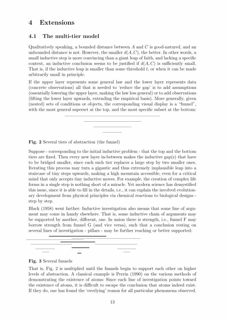
If the upper layer represents some general law and the lower layer represents data(concrete observations) all that is needed to ‘reduce the gap’ is to add assumptions(essentially lowering the upper layer, making the law less general) or to add observations(lifting the lower layer upwards, extending the empirical basis). More generally, given(nested) sets of conditions or objects, the corresponding visual display is a “funnel”,with the most general superset at the top, and the most specific subset at the bottom:

Fig. 2 Several tiers of abstraction (the funnel)

Suppose - corresponding to the initial inductive problem - that the top and the bottomtiers are fixed. Then every new layer in-between makes the inductive gap(s) that haveto be bridged smaller, since each such tier replaces a large step by two smaller ones.Iterating this process may turn a gigantic and thus extremely implausible leap into astaircase of tiny steps upwards, making a high mountain accessible, even for a criticalmind that only accepts tiny inductive moves. For example, the creation of complex lifeforms in a single step is nothing short of a miracle. Yet modern science has demystifiedthis issue, since it is able to fill in the details, i.e., it can explain the involved evolution-ary development from physical principles via chemical reactions to biological designs -step by step.

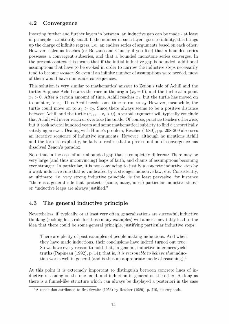
Black (1958) went farther: Inductive investigation also means that some line of argu-ment may come in handy elsewhere. That is, some inductive chain of arguments maybe supported by another, different, one. In union there is strength, i.e., funnel F mayborrow strength from funnel G (and vice versa), such that a conclusion resting onseveral lines of investigation - pillars - may be further reaching or better supported:

Fig. 3 Several funnels

That is, Fig. 2 is multiplied until the funnels begin to support each other on higherlevels of abstraction. A classical example is Perrin (1990) on the various methods ofdemonstrating the existence of atoms: Since each line of investigation points towardthe existence of atoms, it is difficult to escape the conclusion that atoms indeed exist.If they do, one has found the ‘overlying’ reason for all particular phenomena observed.

13

4.2 Convergence

Inserting further and further layers in between, an inductive gap can be made - at leastin principle - arbitrarily small. If the number of such layers goes to infinity, this bringsup the charge of infinite regress, i.e., an endless series of arguments based on each other.However, calculus teaches (or Bolzano and Cauchy if you like) that a bounded seriespossesses a convergent subseries, and that a bounded monotone series converges. Inthe present context this means that if the initial inductive gap is bounded, additionalassumptions that have to be evoked in order to narrow the inductive steps necessarilytend to become weaker. So even if an infinite number of assumptions were needed, mostof them would have minuscule consequences.

This solution is very similar to mathematics’ answer to Zenon’s tale of Achill and theturtle: Suppose Achill starts the race in the origin (x0 = 0), and the turtle at a pointx1 > 0. After a certain amount of time, Achill reaches x1, but the turtle has moved onto point x2 > x1. Thus Achill needs some time to run to x2. However, meanwhile, theturtle could move on to x3 > x2. Since there always seems to be a positive distancebetween Achill and the turtle (xi+1−xi > 0), a verbal argument will typically concludethat Achill will never reach or overtake the turtle. Of course, practice teaches otherwise,but it took several hundred years and some mathematical subtlety to find a theoreticallysatisfying answer. Dealing with Hume’s problem, Rescher (1980), pp. 208-209 also usesan iterative sequence of inductive arguments. However, although he mentions Achilland the tortoise explicitly, he fails to realize that a precise notion of convergence hasdissolved Zenon’s paradox.

Note that in the case of an unbounded gap that is completely different: There may bevery large (and thus unconvincing) leaps of faith, and chains of assumptions becomingever stronger. In particular, it is not convincing to justify a concrete inductive step bya weak inductive rule that is vindicated by a stronger inductive law, etc. Consistently,an ultimate, i.e. very strong inductive principle, is the least pervasive, for instance“there is a general rule that ‘protects’ (some, many, most) particular inductive steps”or “inductive leaps are always justified.”

4.3 The general inductive principle

Nevertheless, if, typically, or at least very often, generalizations are successful, inductivethinking (looking for a rule for those many examples) will almost inevitably lead to theidea that there could be some general principle, justifying particular inductive steps:

There are plenty of past examples of people making inductions. And whenthey have made inductions, their conclusions have indeed turned out true.So we have every reason to hold that, in general, inductive inferences yieldtruths (Papineau (1992), p. 14); that is, it is reasonable to believe that induc-tion works well in general (and is thus an appropriate mode of reasoning).4

At this point it is extremely important to distinguish between concrete lines of in-ductive reasoning on the one hand, and induction in general on the other. As long asthere is a funnel-like structure which can always be displayed a posteriori in the case

4A conclusion attributed to Braithwaite (1953) by Rescher (1980), p. 210, his emphasis.

14

of a successful inductive step, there is no fundamental problem. Generalizing a cer-tain statement with respect to some dimension, giving up a symmetry or subtractinga boundary condition is acceptable, as long as the more abstract situation remainswell-defined.5 The same holds with the improvement of a certain inductive methodwhich is elaborated in Rescher (1980): Guessing an unknown quantity with the help ofReichenbach’s straight rule may serve as a starting point for the development of moresophisticated estimation procedures, based on a more comprehensive understanding ofthe situation. Some of these ‘specific inductions’ will be successful, some will fail.

But the story is quite different for induction in general! Within a well-defined boundedsituation, it is possible to pin down, and thus justify, the move from the (more) specificto the (more) general. However, in total generality, without any assumptions, the end-points of an inductive step are missing. Beyond any concrete model, the upper and thelower tier, defining a concrete inductive leap, are missing, and one cannot expect someinductive step to succeed. For a rationally thinking person, there is no transcendentalreason that a priori protects abstraction (i.e., the very act of generalizing). The essenceof induction is to extend or to go beyond some information basis. This can be done innumerous ways and with objects of any kind (sets, statements, properties, etc.). Thevicious point about this kind of reasoning is that the straightforward, inductively gen-erated expectation that there should be a general inductive principle overarching allspecific generalizations is an inductive leap that fails. It fails since without boundaryconditions - any restriction at all - we find ourselves in the unbounded case, and thereis no such thing as a well-defined funnel there.6

Following this train of thought, Hume’s paradox arises since we confuse a well-defined,restricted situation (line 1 of the next table) with principal doubt, typically accompany-ing an unrestricted framework (or no framework at all, line 2). On the one hand Humeasks us to think of a simple situation of everyday life (the sun rising every morning), ascene embedded in a highly regular scenario. However, if we come up with a reasonable,concrete model for this situation (e.g., a stationary time series), this model will neverdo - since, on the other hand, Hume and many of his successors are not satisfied withany concrete framework. Given any such model, they say, in principle, things couldbe completely different tomorrow, beyond the scope of the model considered. So, nomodel will be appropriate - ever.

Table 1 Bounded vs. unbounded situations

1. concrete model specific prognosis2. no framework no sustained prognosis

Given this, i.e., without any boundary conditions, restricting the situation somehow,we are outside any framework. But without grounds, nothing at all can be claimed,and principal doubt indeed is justified. However, in a sense, this is not fair or rathertrivial: Within a reasonable framework, i.e., given some adequate assumptions, sound

5Also note the elegant symmetry: A set of ‘top down’ boundary conditions is equivalent to the set ofall objects that adhere to all these conditions. Therefore substracting one of the boundary conditionsis equivalent to extending the given set of objects to the superset of all those objects adhering to theremaining boundary conditions.

6An analogy can be found in the universe of sets which is also ordered hierarchically in a naturalway, i.e., with the help of the subset operation (A ⊆ B). Starting with an arbitrary set A, the moregeneral union set A ∪ B is always defined (i.e., for any set B), and so is the inductive gap B\A.However, the union of all sets U no longer is a set. Transcending the framework of sets, it also turnsthe gap U\A into an abyss.

15

conclusions are the rule and not the exception. Outside of any such model, however,reasonable conclusions are impossible. You cannot have it both ways, i.e., request asustained prognosis (first line in table 1), but not accept any framework (second line intable 1). Arguing ‘off limits’ (more precisely, beyond any limit restricting the situationsomehow) can only lead to a principled and completely negative answer.

It should be added that there is also a straightforward logical argument against ageneral inductive principle: A general law is strong, since it - deductively - entailsspecific consequences. Alas, since induction is the opposite of deduction, some generalinductive principle (being the limit of particular inductive rules) would have to beweaker than any specific inductive step. Thus, even if it existed, such a principle wouldbe exceedingly weak and would therefore hardly support anything.

5 Successful inductions

5.1 A paradigmatic large gap: Connecting finite and infinitesequences

Given a finite population of size n, forming the upper layer, and data on k individuals(those that have been observed), there is an inductive gap: The n−k persons that havenot been observed. Closing such a gap is trivial: just extend your data base, i.e., extendthe observations to the persons not yet investigated. Now, since we are dealing withthe problem in a formal way, statistics has no qualms dealing with infinite populations.The upshot of sampling theory is that, even in this case, a rather small, but carefully(i.e., randomly) chosen subset suffices to get ‘close’ to properties (i.e., parameters) ofthe population. It is the standard assumptions built into the statistical paradigm -though seldom mentioned explicitly - that guarantee the convergence of the sample(and its properties) toward the larger population.

Given this, one is back to studying the link between a finite sequence or sample xn =(x1, . . . , xn) on the one hand, and all possible infinite sequences x = x1, . . . , xn, xn+1, . . .,starting with xn on the other. Without loss of generality, we may focus on finite andinfinite binary strings, i.e., xi = 0 or 1 for all i. Thus we have two well defined layers,and we are in the mathematical world. However, there is a fairly large gap to be filled.

Deterministic approach

Kelly (1996) uses the theory of computability (recursive functions) to bridge this enor-mous gap, already encountered by enumerative induction. His approach is mainly topo-logical, and his basic concept is logical reliability. Since “logical reliability demandsconvergence to the truth on each data stream” (ibid., p. 317, my emphasis), his over-all conclusion is rather pessimistic: “. . . classical scepticism and the modern theory ofcomputability are reflections of the same sort of limitations and give rise to demonic ar-guments and hierarchies of underdetermination” (ibid., p. 160). In the worst case, i.e.,without further assumptions (restrictions), the situation is hopeless (see, in particular,his remarks on Reichenbach, ibid., pp. 57-59, 242f).

Not surprisingly, he needs a strong regularity assumption, called ‘completeness’, toget substantial results of a positive nature (ibid., pp. 127, 243): “The characteriza-tion theorems. . .may be thought of as proofs that the various notions of convergence

16

are complete for their respective Borel complexity classes. . .As usual, the proof maybe viewed as a completeness theorem for an inductive architecture suited to gradualidentification.”

Probabilistic approach

Much earlier, de Finetti (1937) had realized that any finite sample contained too lit-tle information to pass to some limit without hesitation. In particular he and otherschallenged the third major axiom of probability theory: If Ai∩Aj = ∅ for all i = j, no-body doubts finite additivity, i.e., p(∪n

i=1Ai) =∑n

i=1 p(Ai). However, mathematiciansneeded, and indeed just assumed, countable additivity: p(∪∞

i=1Ai) =∑∞

i=1 p(Ai).

Kelly (1996) finally gives a reason why the latter assumption has worked so well. Upongiving up logical reliability in favour of probabilistic reliability which “. . . requires onlyconvergence to the truth over some set of data streams that carries sufficiently highprobability” (ibid., p. 317), he realizes that induction becomes much easier to handle.In this (weaker) setting, countable additivity plays the role of a crucial regularity(continuity) condition, guaranteeing that most of the probability mass is concentratedon a finite set. In other words, because of this assumption, one may ignore the endpiece xm+1, xm+2, . . . of any sequence in a probabilistic sense (ibid., p. 324). A ‘nice’consequence is that Bayesian updating, being rather dubious in the sense of logicalreliability (ibid., pp. 313-316), works quite well in a probabilistic sense.

By now it should come as no surprise that “the existence of a relative frequency limitis a strong assumption” (Li and Vitanyi (2008), p. 52). Therefore it is amazing thatclassical random experiments (e.g., successive throws of a coin) straightforwardly leadto laws of large numbers. That is, if x = x1, x2, . . . satisfies certain mild conditions, therelative frequency rn of the ones in the sample xn converges (rapidly) towards r, theproportion of ones in the population. Our overall setup explains why:

First, there is a well-defined, constant population, i.e., an upper tier (e.g., an urnwith a certain proportion r of red balls; some well-defined population parameter, ingeneral). Second, the distance between sample and population is bounded (see section3.3). Third, random sampling connects the tiers in a consistent way. In particular,the probability that a ball drawn at random has the colour in question is r (which, ifthe number of balls in the urn is finite, is Laplace’s classic definition of probability).Because of these assumptions, transition from some random sample to the populationbecomes smooth:

The set S∞ of all binary sequences x, i.e., the infinite sample space, is (almost) equiv-alent to the population (the urn). That is, most of these samples contain r% red balls.(More precisely: The subset of those sequences containing about r% red balls is a setof measure one.) Finite samples xn of size n are less symmetric (Li and Vitanyi (2008),p. 168), in particular if n is small, but no inconsistency occurs upon moving to n = 1,since the probability of a red ball turning up is r.

Conversely, let Sn be the space of all samples of size n. Then, since each finite sequenceof length n can be interpreted as the beginning of some longer sequence, we haveSn ⊂ Sn+1 ⊂ . . . ⊂ S∞. Owing to the symmetry conditions just explained and the well-defined upper tier, increasing n as well as finally passing to the limit does not causeany pathology. Rather, one obtains a law of large numbers (convergence in probabilitytowards a population parameter) or other limit theorems (convergence in distribution),in particular if higher moments of the random variables involved exist.

17

Kolmogorov’s approach

It may be noted that contemporary information theory builds on Kolmogorov complex-ity K(·) rather than probability, not least since with this ingenious concept, the linkbetween the finite and the infinite becomes particularly elegant: First, some sequencex = x1, x2, . . . with initial segment xn = (x1, . . . , xn) is called algorithmically randomif its complexity grows fast enough, i.e., if the series

∑n 2

n/2K(xn) is bounded (Li andVitanyi (2008), p. 230). Second, x is algorithmically random if and only if “the com-plexity of each initial segment is at least its length.” (ibid., p. 221). In plain Englishthe theorem just stated says that one is able to move from random (very complex)finite vectors to random infinite series - and back - seamlessly: Both possess ‘almost’maximum Kolmogorov complexity.7

Finally, it should be mentioned that the theory is able to explain the remarkablephenomenon of a “practical limit” or “apparent convergence” without reference to a(real) limit: Most finite binary strings have high Kolmogorov complexity, i.e., they arevirtually incompressible. According to Fine’s theorem (cf. Li and Vitanyi (2008), pp.141), the fluctuations of the relative frequencies of these sequences are small. Bothfacts combined explain “why in a typical sequence [. . .] the relative frequencies appearto converge or stabilize. Apparent convergence occurs because of, and not in spite of,the high irregularity (randomness or complexity) of a data sequence” (ibid., p. 142).

In a nutshell: A “practical limit” is the rule, but real convergence is the exception, sincethe latter property is a strong assumption (i.e. there are only relatively few sequencesthat have this property). Thus Reichenbach’s ‘pragmatic justification’ of induction isa red herring, apparent convergence being thoroughly misleading.

5.2 Coping with circularity

All verbal arguments of the form “Induction has worked in the past. Is that goodreason to trust induction in the future?” or “What reason do we have to believe thatfuture instances will resemble past observations?” have more than an air of circularityto them. If I say that I believe in the sun rising tomorrow since it has always risen inthe past, I seem to be begging the question. More generally: Inductive arguments areplagued by the reproach that they are, essentially, circular.

Given a sequential interpretation, suppose we use all the information I(n) that hasoccurred until day n in order to proceed to day n+1. It seems to be viciously circularto use all the information I(n−1) that has occurred until day n−1 in order to proceedto day n, etc. However, partial recursive functions (loops), very popular in computerprogramming, demonstrate that this need not be so:

n!, called “n factorial”, is defined as the product of the first n natural numbers, thatis n! = 1 · 2 · · ·n, for instance 4! = 1 · 2 · 3 · 4 = 24. Now, consider the program

FACTORIAL[n]:

• IF n = 1 THEN n! = 1

7The complete theory is developed in Li and Vitanyi (2008), chapters 2.4, 2.5, 3.5, and 3.6. Theirchapter 1.9 gives a historical account, explicitly referring to von Mises, the ‘father’ of Frequentism.Since any regularity is a kind or redundancy that can be used to compress a given string of data, thebasic idea is to identify incompressibility with randomness: (almost) incompressible ≈ highly complex≈ algorithmically random.

18

• ELSE n! = n· FACTORIAL[n− 1]

At first sight, this looks viciously circular, since ‘factorial is explained by factorial.’That is, the factorial function appears in the definition of the factorial function, andit is used to calculate itself. One should think that, for a definition to be proper, atthe very least, some object (such as a specific function) must not be defined with theexplicit help of this very object. Yet, as a matter of fact, the second line of the programimplicitly defines a loop that is evoked just a finite number of times. For instance,

4! = 4 · 3! = 4 · 3 · 2! = 4 · 3 · 2 · 1! = 4 · 3 · 2 · 1 = 24.

The point is that, on closer inspection, the factorial function depends on n. Everytime the program FACTORIAL[·] is evoked, a different argument is inserted, and sincethe arguments are natural numbers descending monotonically, the whole procedureterminates after a finite number of steps. Shifting the problem from the calculation ofn! to the calculation of (n− 1)! not only defers the problem, but also makes it easier.Because of boundedness, this strategy leads to a well-defined algorithm, calculating thedesired result.

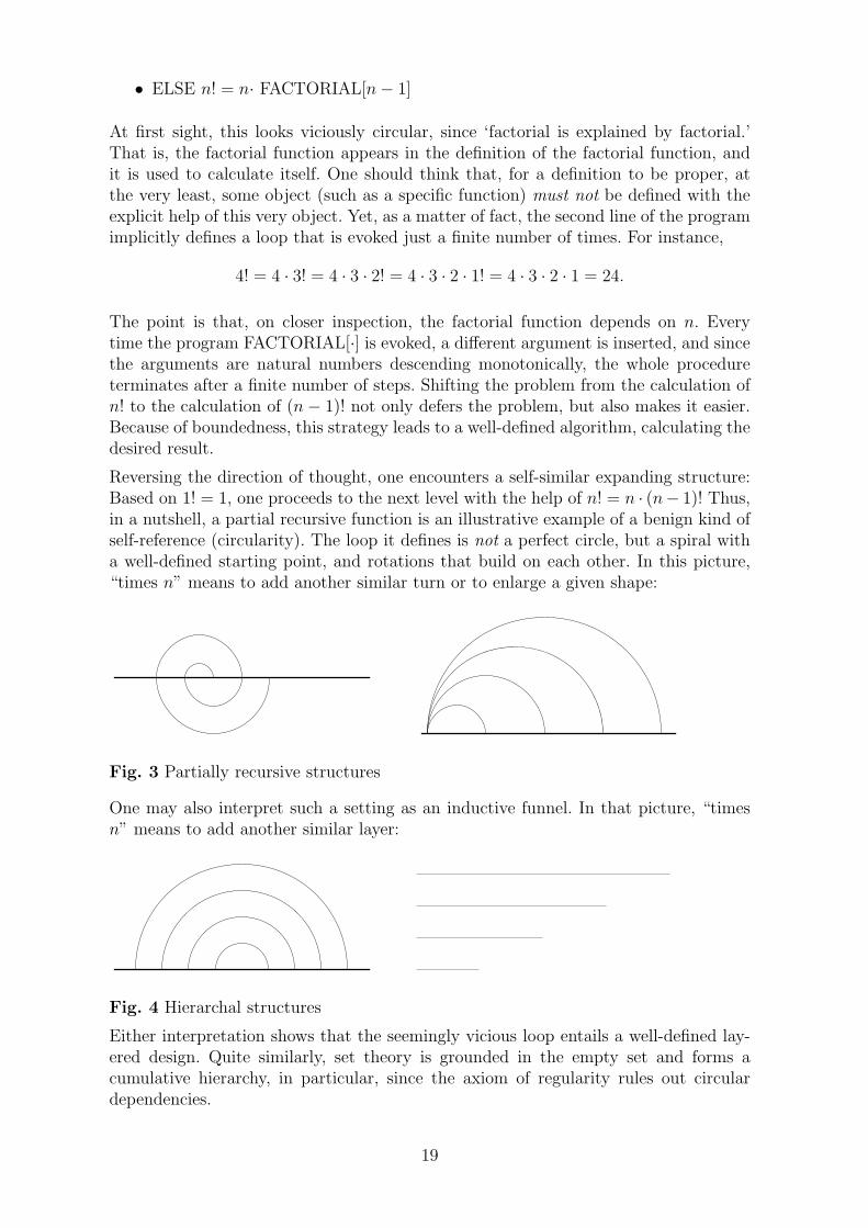
Reversing the direction of thought, one encounters a self-similar expanding structure:Based on 1! = 1, one proceeds to the next level with the help of n! = n · (n− 1)! Thus,in a nutshell, a partial recursive function is an illustrative example of a benign kind ofself-reference (circularity). The loop it defines is not a perfect circle, but a spiral witha well-defined starting point, and rotations that build on each other. In this picture,“times n” means to add another similar turn or to enlarge a given shape:

Fig. 3 Partially recursive structures

One may also interpret such a setting as an inductive funnel. In that picture, “timesn” means to add another similar layer:

Fig. 4 Hierarchal structures

Either interpretation shows that the seemingly vicious loop entails a well-defined lay-ered design. Quite similarly, set theory is grounded in the empty set and forms acumulative hierarchy, in particular, since the axiom of regularity rules out circulardependencies.

19

The latter perspective demonstrates that using the information I(n) in order to get toI(n + 1) need not be viciously circular. If I(n) < I(n + 1) for all natural numbers n,there is no ‘vicious’ circularity, but rather a many-layered hierarchy. Thus, it is not alogical fallacy to evoke “the sun has risen n times” in order to justify “the sun will risen+1 times.” Only if the assumptions were at least as strong as the conclusions, i.e., inthe case of a tautology or a deductive argument, would one be begging the question.

However, we are dealing with induction, i.e., the fact that the sun has risen untiltoday does not imply that it will rise tomorrow. In other words, there are inevitableinductive gaps, a sequence of assumptions that become weaker and weaker: I(n) beingbased on I(n−1), being based on I(n−2), etc. This either leads to a finite chain (e.g.,I(1) representing the first sunrise), or to a sound convergence argument (discussed insubsection 4.2), since information is non-negative.

Starting with day 1, instead, evidence accrues. That is, I(1) ≤ I(2) ≤ . . . ≤ I(n), andI(n) may be considerably larger than I(1). Of course, if the gaps I(k + 1) − I(k) arelarge, this way to proceed might not necessarily be convincing, but that is a differentquestion.

Quantitative considerations

An appropriate formal model for the latter example is the natural numbers (corre-sponding to days 1, 2, 3, etc.), having the property Si that the sun rises on this day.That is, Si = 1 if the sun rises on day i, and Si = 0 otherwise.

Given the past up to day n with Si = 1 for all i ≤ n, the inductive step consistsin moving to day n + 1. In a sense, i.e., without any further assumptions, we cannotsay anything about Sn+1, and of course Sn+1 = 0 is possible. However, if we usethe sequential structure and acknowledge that information accrues it seems to be areasonable idea to define the inductive gap, when moving from day n to day n+ 1, asthe fraction

n+ 1

n= 1 +

1

nIn other words, if each day contributes the same amount of information (1 bit), 1/n isthe incremental gain of information. Quite obviously, the relative gain of informationgoes to 0 if n → ∞.

The above may look as though the assumption of “uniformity of nature” (associatedwith circularity) had to be evoked in order to get from day n to day n + 1. However,this is not so. First, since the natural numbers are a purely formal model, some naturalphenomenon like the sun rising from day to day is merely used as an illustration.Second, although the model can be interpreted in a sequential manner one need notdo so. One could also say: Given a sample of size n, what is the relative gain of addinganother observation? The answer is that further observations provide less and lessinformation relative to what is already known. It is the number of objects alreadyobserved that is crucial, making the proportion larger or smaller: Adding 1 observationto 10 makes quite an impact, whereas adding 1 observation to a billion observationsdoes not seem to be much.

Laplace (1812), who gave a probabilistic model of the sunrises, argued along the samelines and came to a similar conclusion. Since every sunrise contributes some informa-tion, the conditional probability that the sun will rise on day n + 1, given that it hasalready risen n times should be an increasing function in n. Moreover, since the relativegain of information becomes smaller, the slope of this function would decrease mono-

20

tonically. Laplace’s calculations yielded p(Sn+1|S1 = . . . = Sn = 1) = (n + 1)/(n + 2)which, as desired, is an increasing and concave function in n. This model only usesthe information given by the data (i.e., the fact that the sun has risen n times in suc-cession). He noted that the probability becomes (much) larger, if further informationabout our solar system is taken into account.

Asymptotic information theory

One might object that the physical principle of “uniformity of nature” is replaced bythe (perhaps equally controversial) formal principle of “indifference”, i.e., that eachobservation is equally important or carries the same “weight” w ≥ 0. But that is nottrue either. For even if the observations carry different weights wi ≥ 0, the conclusionthat further data points become less and less important remains true in expectation:Given a total of n observations, their sum of weights w.l.o.g. being 1, the expectedweight of each of these observations has to be 1/n. Thus we expect to collect theinformation I(k) = k/n with the first k observations, and the expected relative gain ofinformation that goes with observation k + 1 still is ∆(k) = I(k + 1)/I(k) = k+1

n/ kn=

k+1k

= 1 + 1/k.

To make ∆(n) large, one would have to arrange the weights in ascending order. How-ever, ‘save the best till last’ is just the opposite to some typical scenario that can beexpected for reasons of combinatorics. Uniformity in the sense of an (approximate) uni-form distribution is a mere consequence of these considerations due to the asymptoticequipartition property (see, e.g., Cover and Thomas (2006)), chap. 3. Rissanen (2007),p. 25, explains:

As n grows, the probability of the set of typical sequences goes to one atthe near exponential rate . . . Moreover . . . all typical sequences have justabout equal probability.

It may be added that “non-uniformity” in the sense that the next observation could becompletely different from all the observations already known cannot occur in the abovemodel, since every observation only has a finite weight wi which is a consequence ofthe fact that the sum of all information is modelled as finite (w.l.o.g. equal to 1).

In general, i.e., without such a bound, the information I(A) of an event A is a mono-tonically decreasing and continuous function of its probability. Thus if the proba-bility is large, the surprise (amount of information) is little, and vice versa. In theextreme, p(A) = 1 ⇔ I(A) = 0 (some sure event is no surprise at all), but alsop(A) = 0 ⇔ I(A) = ∞. That is, if something deemed impossible happens, I = ∞indicates that the framework employed is wrong.

5.3 Invertibility

Throughout this contribution, and perfectly in line with the received framework, in-ductive problems involve (at least) two levels of abstraction being connected in anasymmetric way. If these levels are coupled together with the help of a certain opera-tion, the classical issue of inferring a general pattern from the observation of particularinstances translates into models consisting of two layers and an asymmetric relationbetween them. Consistently, the most primitive of such models is defined by two setsA,C, connected by the subset relation ⊆. The corresponding operation that simplifies

21

matters (wastes information) is a non-injective mapping f : A → C. In other words,there are elements a ∈ A having the same image c = f(a) in C, and the size of the setof all members of A that are mapped to an ‘non-exclusive’ c ∈ C is a natural measureof the mapping’s invertibility. In the extreme, all a ∈ A are mapped to a single c, sothat, given c it is impossible to say anything about this observation’s origin.

Neglecting the layers and focussing on the operation, it is always possible to proceedfrom the more abstract level (containing more information) to the more concrete situ-ation (containing less information). This step may be straightforward or even trivial.Typically, the corresponding operation simplifies matters and there are thus generalrules governing this step (e.g., adding random bits to a certain string, conducting arandom experiment, executing an algorithm, differentiating a function, making a state-ment less precise, etc.). Taken with a pinch of salt, this direction may thus be calleddeductive.

Yet the inverse inductive operation is not always possible or well-defined. It only existssometimes, given certain additional conditions, in specific situations. Even if it exists,it may be impossible to find it in a rigorous or mechanical way. For example, there isno general algorithm to compress an arbitrary string to its minimum length, objectscan exist but may not be constructible, and it can be very difficult to find a causalrelationship behind a cloud of correlations. Consistently, Bunge (2019) emphasizes that“inverse problems” are much more difficult than “forward problems.”

In general, there is a continuum of reversibility: One extreme is perfect reversibility,i.e., given some operation, its inverse is also always possible. For example, + and -are perfectly symmetric. If you can add two numbers, you may also subtract them.That is not quite the case with multiplication, however. On the one hand, any twonumbers can be multiplied, but on the other hand, all numbers except one (i.e., thenumber 0) can be used as a divisor. So, there is almost perfect symmetry with 0being the exception. Typically, an operation can be partially inverted. That is, f−1 canbe explained given some special conditions. These conditions can be non-existent (anydifferentiable function can be integrated), mild (division can almost always be applied),or quite restrictive (in general, ab is only defined for positive a).

Thus, step by step, we arrive at the other extreme: perfect non-reversibility, i.e., anoperation cannot be inverted at all. For example, given a sequence x = x1, x2, x3, . . .,it is trivial to proceed to xn = (x1, . . . , xn), since one simply has to skip xn+1, xn+2, . . .However, without further assumptions, it is impossible to infer anything about xn’ssuccession. Although the operation (link) between x and xn is just a well-defined pro-jection, it is also a so-called “trapdoor function.” That is, having traveled through thisdoor, it is impossible to get back, since the distance between the finite and the infinitesituations (the floor and the ceiling so to speak) is unbounded.

Cases near the latter pole lend credibility to Hume’s otherwise amazing claim that onlydeduction can be rationally justified, or that induction does not exist at all (Popper).Yet there is a large middle ground held by “partial invertibility.” For example, Knight(1921), p. 313, says:

The existence of a problem in knowledge depends on the future being differ-ent from the past, while the possibility of a solution of the problem dependson the future being like the past.

22

Probability theory and statistics

Upon trying to solve Hume’s problem, many philosophers - most notably Reichenbach,Carnap, Popper, and the Bayesian school (Howson und Urbach 2006) - have looked toprobability and statistics. A major reason could be that invertibility is quite straight-forward in that area:

Given some set Ω, the first axiom of probability states that p(Ω) = 1, i.e., that thetotal probability mass is bounded. Therefore, if you know the probability p(A) of someevent A, you may straightforwardly compute the probability of the opposite event A,since p(A) = 1− p(A).

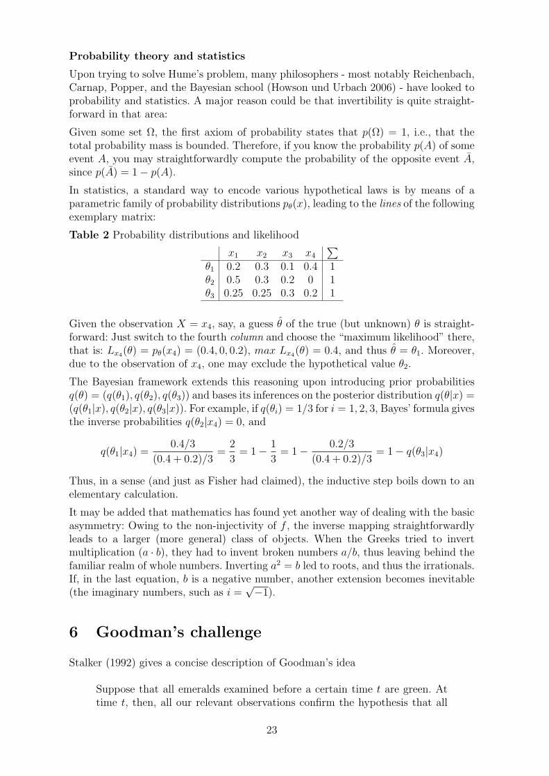
In statistics, a standard way to encode various hypothetical laws is by means of aparametric family of probability distributions pθ(x), leading to the lines of the followingexemplary matrix:

Table 2 Probability distributions and likelihood

x1 x2 x3 x4

∑θ1 0.2 0.3 0.1 0.4 1θ2 0.5 0.3 0.2 0 1θ3 0.25 0.25 0.3 0.2 1

Given the observation X = x4, say, a guess θ of the true (but unknown) θ is straight-forward: Just switch to the fourth column and choose the “maximum likelihood” there,that is: Lx4(θ) = pθ(x4) = (0.4, 0, 0.2), max Lx4(θ) = 0.4, and thus θ = θ1. Moreover,due to the observation of x4, one may exclude the hypothetical value θ2.

The Bayesian framework extends this reasoning upon introducing prior probabilitiesq(θ) = (q(θ1), q(θ2), q(θ3)) and bases its inferences on the posterior distribution q(θ|x) =(q(θ1|x), q(θ2|x), q(θ3|x)). For example, if q(θi) = 1/3 for i = 1, 2, 3, Bayes’ formula givesthe inverse probabilities q(θ2|x4) = 0, and

q(θ1|x4) =0.4/3

(0.4 + 0.2)/3=

2

3= 1− 1

3= 1− 0.2/3

(0.4 + 0.2)/3= 1− q(θ3|x4)

Thus, in a sense (and just as Fisher had claimed), the inductive step boils down to anelementary calculation.

It may be added that mathematics has found yet another way of dealing with the basicasymmetry: Owing to the non-injectivity of f , the inverse mapping straightforwardlyleads to a larger (more general) class of objects. When the Greeks tried to invertmultiplication (a · b), they had to invent broken numbers a/b, thus leaving behind thefamiliar realm of whole numbers. Inverting a2 = b led to roots, and thus the irrationals.If, in the last equation, b is a negative number, another extension becomes inevitable(the imaginary numbers, such as i =

√−1).

6 Goodman’s challenge

Stalker (1992) gives a concise description of Goodman’s idea

Suppose that all emeralds examined before a certain time t are green. Attime t, then, all our relevant observations confirm the hypothesis that all

23

emeralds are green. But consider the predicate ‘grue’ which applies to allthings examined before t just in case they are green and to other things justin case they are blue. Obviously at time t, for each statement of evidence as-serting that a given emerald is green, we have a parallel evidence-statementasserting that that emerald is grue. And each evidence-statement that agiven emerald is grue will confirm the general hypothesis that all emeraldsare grue [. . .] Two mutually conflicting hypotheses are supported by thesame evidence.

In view of the funnel-structure discussed throughout this contribution, this bifurcationis not surprising. However, there is more to it:

And by choosing an appropriate predicate instead of ‘grue’ we can clearlyobtain equal confirmation for any prediction whatever about other emer-alds, or indeed for any prediction whatever about any other kind of thing.

In other words, instead of criticizing induction like so many of Hume’s successors,Goodman’s innovative idea is to trust induction, and to investigate what happens next.Unfortunately, induction’s weakness thus shows up almost immediately: It is not at allobvious in which way to generalize a certain statement - which feature is ‘projectable’which is not (or to what extent)? For example, this line of argument may “lead to theabsurd conclusion that no experimenter is ever entitled to draw universal conclusionsabout the world outside his laboratory from what goes on inside it.” (ibid.)

In a nutshell, if we do not trust induction, we are paralysed, not getting anywhere.However, if we trust induction, this method could take us anywhere, which is almostequally disastrous. In our basic model, these cases correspond to d(A,C) = 0, andd(A,C) = ∞, respectively.

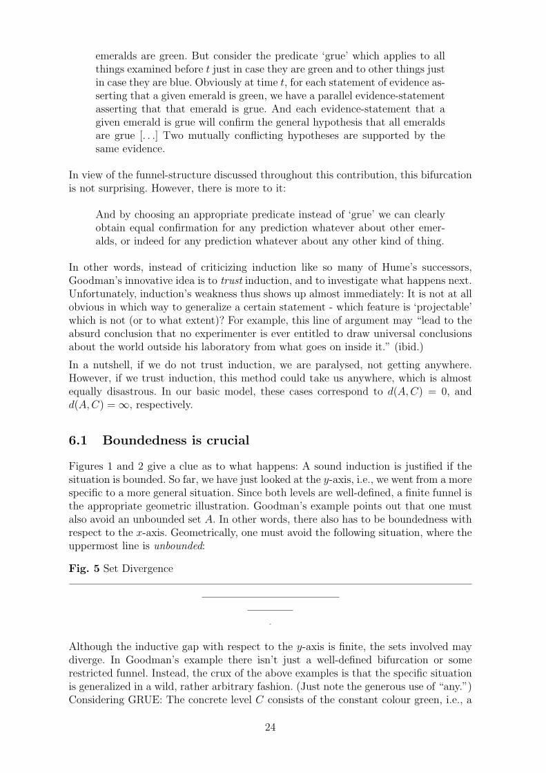
6.1 Boundedness is crucial

Figures 1 and 2 give a clue as to what happens: A sound induction is justified if thesituation is bounded. So far, we have just looked at the y-axis, i.e., we went from a morespecific to a more general situation. Since both levels are well-defined, a finite funnel isthe appropriate geometric illustration. Goodman’s example points out that one mustalso avoid an unbounded set A. In other words, there also has to be boundedness withrespect to the x-axis. Geometrically, one must avoid the following situation, where theuppermost line is unbounded:

Fig. 5 Set Divergence

Although the inductive gap with respect to the y-axis is finite, the sets involved maydiverge. In Goodman’s example there isn’t just a well-defined bifurcation or somerestricted funnel. Instead, the crux of the above examples is that the specific situationis generalized in a wild, rather arbitrary fashion. (Just note the generous use of “any.”)Considering GRUE: The concrete level C consists of the constant colour green, i.e., a

24

single point. The abstract level A is defined by the time t a change of colour occurs.This set has the cardinality of the continuum and is clearly unbounded. It would sufficeto choose the set of all days in the future (1 = tomorrow, 2 = the day after tomorrow,etc.) indicating when the change of colour happens, and to define t = ∞ if there isno change of colour. Clearly, the set IN ∪ ∞ is also unbounded. In both models wewould not know how to generalize or why to choose the point ∞.

Here is a practically relevant variation: Suppose we have a population and a large(and thus typical) sample. This may be interpreted in the sense that, with respect tosome single property, the estimate θ is close to the true value θ in the population.However, there is an infinite number of (potentially relevant) properties, and with highprobability, the population and the sample will differ considerably in at least one ofthem. Similarly, given a large enough number of nuisance factors, at least one of themwill thwart the desired inductive step from sample to population, the sample not beingrepresentative of the population in this respect.

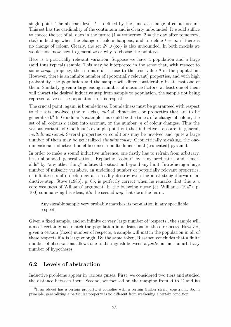
The crucial point, again, is boundedness. Boundedness must be guaranteed with respectto the sets involved (the x−axis), and all dimensions or properties that are to begeneralized.8 In Goodman’s example this could be the time t of a change of colour, theset of all colours c taken into account, or the number m of colour changes. Thus thevarious variants of Goodman’s example point out that inductive steps are, in general,multidimensional. Several properties or conditions may be involved and quite a largenumber of them may be generalized simultaneously. Geometrically speaking, the one-dimensional inductive funnel becomes a multi-dimensional (truncated) pyramid.

In order to make a sound inductive inference, one firstly has to refrain from arbitrary,i.e., unbounded, generalizations. Replacing “colour” by “any predicate”, and “emer-alds” by “any other thing” inflates the situation beyond any limit. Introducing a hugenumber of nuisance variables, an undefined number of potentially relevant properties,or infinite sets of objects may also readily destroy even the most straightforward in-ductive step. Stove (1986), p. 65, is perfectly correct when he remarks that this is acore weakness of Williams’ argument. In the following quote (cf. Williams (1947), p.100) summarizing his ideas, it’s the second any that does the harm:

Any sizeable sample very probably matches its population in any specifiablerespect.

Given a fixed sample, and an infinite or very large number of ‘respects’, the sample willalmost certainly not match the population in at least one of these respects. However,given a certain (fixed) number of respects, a sample will match the population in all ofthese respects if n is large enough. By the same token, Rissanen concludes that a finitenumber of observations allows one to distinguish between a finite but not an arbitrarynumber of hypotheses.

6.2 Levels of abstraction

Inductive problems appear in various guises. First, we considered two tiers and studiedthe distance between them. Second, we focused on the mapping from A to C and its

8If an object has a certain property, it complies with a certain (rather strict) constraint. So, inprinciple, generalizing a particular property is no different from weakening a certain condition.

25

inverse. While the symmetric concept of distance highlights the similarity of A and C;the inverse function, logical implication, and the subset-relation are all asymmetric,and thus point at the difference.9

Although such a clear separation is more transparent than some notion of “partialinvertibility” that easily confounds both perspectives, Goodman’s challenge hints atanother, a third class of problems: Given a concrete sample C - what could be areasonable generalization A (plus a natural mapping connecting these tiers)?

In other words: Starting with some piece of information, very often the most seriousproblem consists in finding a suitable level of abstraction. Having investigated someplatypuses in zoos, it seems to be a justified conclusion that they all lay eggs (since theyall belong to the same biological species), but not that they all live in zoos (since therecould be other habitats populated by platypuses). In Goodman’s terms, projectibilitydepends on the property under investigation. Depending on the specific situation, itmay be non-existent or (almost) endless. The stance taken so far is that as long as thereis a bounded funnel-like structure in every direction of abstraction, the inductive stepstaken are rational. The final result of a convincing inductive solution always consistsof the sets (objects), dimensions (properties) and boundary conditions involved, plus(at least) two levels of abstraction in each dimension.

Given just C, however, the difficulty is twofold: First, one always has to construct A,i.e., A is not given. Second, upon constructing A, there is the problem of determining areasonable distance d(A,C). On the one hand, a critical attitude (distrust) easily leadsto d(A,C) = 0. On the other hand, an optimistic point of view (trust in induction)straightforwardly results in d(A,C) = ∞. Moreover, in the worst case scenario, just asingle finite d(A,C) will do - we should claim neither more nor less. This is as subtle aproblem as sending a satellite into orbit: If the impetus is too weak, it will come downagain; if the impetus is too strong, it will disappear.

Thinking of “projectibility” and its opaqueness, there may be specific answers in certainscenarios. But be this as it may, is there a general answer without reference to asemantic context? In section 3.2, the discussion of Rissanen’s example already hintedat the general solution given by the information sciences. Informally,

Prior information + Information in some set of data = Posterior information

Formally, the information of some event is just the negative logarithm of its probability.Therefore adding information is tantamount to multiplying probabilities. If the eventsare a hypothesis H and data x we get

I(H,x) = I(H) + I(x|H) ⇔ − log p(H,x) = − log p(H)− log p(x|H)

⇔ p(H,x) = p(H) · p(x|H) (1)

In other words: The first tier C consists of the prior hypothesis H, the second tierA is the more detailed information available after having seen the data x, consistingof H and x. The difference is just the information in the data which is not alreadycontained in H. (Things that are known do not need to be learned twice.) The stepfrom prior to posterior is inductive in the sense that a vague picture becomes more

9Quite similarly, in information theory, mutual information I(A,C) is a fundamental symmetricconcept, and KL-divergence, being at least as important, is asymmetric (Cover and Thomas 2006).

26

detailed. Notice, that (1) does not generalize from the data to the hypothesis, butrather from the hypothesis to the hypothesis plus the data.

Qualitatively speaking, it is not obvious how much “distance” is bridged by the data.If the distance I(x|H) were too small, we would not use all the information available.Thus we would lose if we played against somebody using all the information at hand.If I(x|H) were too large, we would go too far, i.e., a part of the conclusion could not besubstantiated with the help of the data, amounting to a real inductive (non-deductive)step. Thus, somebody using just the amount of information truly available - but nomore - would also beat us if we gambled.

In other words, there is a unique logically sound solution: Prior information I(H) andthe information in the data conditional on the prior I(x|H) must add up to the totalinformation I(H,x) which is equation (1). Traditionally, the gambling schemes justintroduced are known as Dutch books. It is only possible to avoid them if the decisionsof a gambler are consistent, i.e., if he adheres to the axioms of probability theory(Ramsey 1926, de Finetti 1937, Greenland 1998) which is also reflected in (1). Finally,symmetrizing equation (1) immediately yields Bayes’ formula

p(B|A) · p(A) = p(A,B) = p(A|B) · p(B) ⇔ p(A|B) =p(B|A) · p(A)

p(B)

with general events A,B. Therefore it seems to be no coincidence that Bayesians areamong the most ardent defenders of induction.

Note that Rissanen’s notion of ‘optimal distinguishability’ implements the same idea:Given some set of data, i.e., a certain amount of information, there is a correspondingmaximum number of rationally distinguishable hypotheses. In a simplistic manner, onecould say that one needs more/less data in order to differentiate between more/fewerhypotheses.

7 Summary

In sum, at least formally, Hume’s problem can be dealt with in a constructive way.It turns out that the key concepts are boundedness and information. If the mutualinformation or distance between A and C is larger than zero, it is possible to saysomething about C given A - and vice versa! To this end, there has to be a linkbetween A and C. In theoretical settings the logical link necessary is provided bysome assumption. Hume (1748/2008) was right in noticing that a strong condition like‘resemblance’ may easily be violated. However, a weak kind of concatenation may alsosuffice for an educated guess.

In principle almost any kind of coupling will do, as long as the link transports someinformation. Here is a straightforward counterexample: If information flows from C toA but not from A to C (i.e., given a trapdoor function or an invisible observer in thesky), A is able to learn something about C, but not vice versa. Arguably, the moststraightforward way to model a linkage between two sets is the subset relation, i.e.,C ⊆ A, or, almost equivalently, to consider a sample C from some population A. In theeasiest case, it is just the cardinality of the sets that is relevant. More precisely, if |M |denotes the cardinality of some set M , and C ⊆ A, the larger the ratio |C|/|A|, themore one knows about A, given the sample C. In particular, if A = C ⇒ |C|/|A| = 1,

27

there is no inductive problem; if |C| = 0, i.e., if there is no sample from A, nothingcan be said about A. Enumerative induction is not convincing since in this case |C| isa finite number, but |A| = ∞. However, as long as the ratio |C|/|A| remains finite, itseems fair to say that there is some evidence in C about A, and the closer |C|/|A| isto one, the stronger this evidence is.

A more sophisticated model should distinguish between cardinality and information.The most straightforward formalization could be C ⊆ A and I(C) < I(A). Given thissituation, there are three ways to proceed:

(i) Deductively, i.e., from A to C.

(ii) Inductively, i.e., from C to A, leaping over a gap of size I(A)− I(C).

(iii) Additively, i.e., I(C) + d = I(A), with d > 0 bridging the gap, see equation (1).

More generally speaking, a model should formalize IA(C), the information in C aboutsome property or parameter of A. In statistics, C is represented by a sample and Ais some population. Bad samples and difficult estimation problems have in commonthat IA(C) is low, although the size of the sample might be considerable. In the worstcase, IA(C) is minute, despite the fact that |C| and |A| do not differ much.10 This iswhere random sampling comes in: For combinatorial reasons, typically IA(C) is large,although the size of the sample may still be rather small.

All in all, statistics provides the most comprehensive response to Hume’s problem:Given its basic sample-population model, standard assumptions guarantee convergence(LLN etc.) Given the link between probability and information, one may calculate howto proceed from C to A (information adds up, probabilities multiply, and Bayesianupdating is the standard way to include new information). Finally, the axioms of prob-ability provide a sound foundation for probability calculations, exclude Dutch books(inconsistency) and underpin rationality. On top of this, countable additivity essen-tially reduces infinite sequences to finite samples. Thus these considerations combinedpin down the crucial ingredients of the problem and provide constructive answers.

Alas, it is quite typical for verbal discussions that they easily miss their target. Thewhole philosophical discussion seems to revolve around the “rhetoric of independence”(cf. Stove (1986), Ch. VIII). That is, at the end of the day, all arguments in favour of in-duction tend to be unconvincing, since the observed and the unobserved are “loose andseparate”, “disjoint”, “lack connection”, etc. However, consider deterministic chaos: Al-though there exists a deterministically strong connection (i.e., if you know the presentstate x of the system, you also know its future state y = f(x)), the mapping f alsoscatters the points of any neighbourhood U(x) of x so effectively that prediction be-comes a futile endeavour. So, in a sense, the link between the present and the futureis strong and weak simultaneously, and one may easily bark up the wrong tree.

Instead, the crucial point - again - is unboundedness: The information at present, nomatter how detailed, decays exponentially, leaving no ground for a rational prediction.

10If every observation contributes (about) the same amount of information, all samples of size n areequivalent in the sense that they contain (about) the same amount of information. In other words, insuch ‘nice’ situations, quite typical for classical statistics, there are neither good nor bad samples. Allthat matters is the size n of the sample (the larger n the better). This is not so in difficult estimationproblems, when a few of the observations contain most of the information. Thus information does notaccrue steadily. Rather, there are a few sudden jumps. In the most extreme case, all depends on asingle and thus crucial observation.

28

Equivalently, one can say that uncertainty (errors) grows very fast, soon exceedingany bound. In this view, Hume’s stance amounts to the remarkable claim that the‘predictive horizon’ is precisely zero, no exception. In other words: Scepticism in itsmost extreme form (i.e., rational prediction is strictly impossible) is tantamount toevery bit of information always vanishing instantaneously.

However, Hume was right that there is no such thing as a free lunch (NFL). Withoutany assumptions, boundary conditions or restrictions - beyond any bounds - there areno grounds for induction. Indeed, it has been possible to prove various “NFL theorems”in the field of machine learning (Wolpert 2013), for instance “. . . just because ProfessorSmith produces search algorithms that outperform random search in the past, withoutmaking some assumption about the probability distribution over universes, we cannotconclude that they are likely to continue to do so in the future” (ibid., p. 7).

Induction only works within certain frameworks, e.g., those of statistics. Groarke(2009), p. 61, makes a similar point: “Yes, post-Cartesian scepticism undermines in-ductive reasoning, but it also undermines deduction and everything else. This kind ofabsolute doubt, consistently practiced, makes genuine knowledge impossible.” It maybe conceded, however, that crucial assumptions are often kept implicit, thus we hadto dig deep into technical details to expose them. Without these boundary conditions,the information sciences - at least their asymptotic theories - would not work.

For more on these matters see Saint-Mont (2017). Apart from being more compre-hensive, that work also discusses many historical attempts and the empirical side toinduction. In particular: why are we “dealing with an ‘inductively normal’ world - aworld in which induction is an actually efficient mode of inquiry” (Rescher (1980),pp. 160-161)? Why are inductive leaps, typically, ‘predictively reliable’ or why do theypossess, in Peirce’s words, a ‘truth-producing virtue’ (cf. Braithwaite (1953), p. 264)?

Following the above train of thought, the roundabout answer seems to be that persist-ing patterns are the rule. That is, in the world we inhabit and in most of our models,information decays rather slowly (Costa (2018), pp. 357-359); and if information is atleast conserved to some extent, predictions are feasible. Acknowledging that objects,forms and regularities are particular and particularly important expressions of infor-mation, it is structure - which may be understood as preserved information - ratherthan conformity that is crucial: One can have reasonable doubts in nature’s uniformity,however, hardly anybody will challenge the fact that we live in a structured universe.

In sum, inductive steps can often be justified, boundedness and information beingthe crucial ideas, essentially leading to ‘inductive funnels’ (see the illustrations). Inparticular, convergence and (partially) recursive functions demonstrate that inductionis far from worthless circular reasoning. Given any reasonable framework, inductivesteps can be vindicated, i.e., Hume’s remarkable claim that no inductive step is everjustified seems to be hardly more than an ‘old wives’ tale.’ Reality chooses to be withcautious hierarchal non-circular inductive steps, rather than with principled doubt.

29

References

Baum, L.E.; Katz, M.; and R.R. Read (1962). Exponential convergence rates for thelaw of large numbers. Trans. Amer. Math. Soc. 102, 187-199.

Black, M. (1958). Self-supporting inductive arguments. J. of Phil., 55(17), 718-725.

Braithwaite, R.B. (1953/68). Scientific explanation. Cambridge: At the university press.Partly reprinted as chap. 7 in Swinburne (1974), 102-126.

Broad, C.D. (1952). The philosophy of Francis Bacon. In: Ethics and the history ofphilosophy. London: Routledge and Kegan Paul.

Bunge, M. (2019). Inverse problems. Foundations of Science, 24, 483-525.

Campbell, S. (2001). Fixing a Hole in the Ground of Induction. Australasian Journalof Philosophy, 79(4), 553–563.

Campbell, S.; and J. Franklin (2004). Randomness and the Justification of Induction.Synthese, 138(1), 79–99.

Costa, C. (2018). Philosophcial Semantics. Reintegrating theoretical philosophy. New-castle upon Tyne: Cambridge Scholars Publishing.

Cover, T.M.; and Thomas, J.A. (2006). Elements of Information Theory. (2nd ed.) NewYork: Wiley.

Finetti, B. de (1937). La Prevision: ses Lois Logiques, ses Sources Sujectives. Ann. Inst.H. Poincare 7, 1-68.

Encylopedia Britannica (2018). Induction. www.britannica.com/topic/induction-reason

Erdi, P. (2008). Complexity explained. Berlin, Heidelberg: Springer.

Fazekas, I.; and O.I. Klesov (2000). A general approach to the strong laws of largenumbers. Teor. Veroyatnost. i Primenen. 45(3), 568–583; Theory Probab. Appl.,45(3) (2002), 436–449.

Fisher, R.A. (1966). The Design of Experiments. (8th ed.). New York: Hafner Publish-ing Company.

Gauch, H.G. Jr. (2012). Scientific method in brief. Cambridge: Cambridge Univ. Press.

Greenland, S. (1998). Probability Logic and Probabilistic Induction. Epidemiology9(3), 322-332.

Godfrey-Smith, P. (2003). Theory and Reality. Chicago and London: The Universityof Chicago Press.

Groarke, L. (2009). An Aristotelean account of induction. Montreal: McGill-Queen’sUniversity Press.

Hacking, I. (2001). An Introduction to Probabilty Theory and Inductive Logic. Cam-bridge: Cambridge University Press, Cambridge.

30

Howson, C.; and Urbach, P. (2006). Scientific Reasoning. The Bayesian Approach (3rded.). Open Court, Chicago and La Salle, IL.

Hume, D. (2008). 1st ed. 1748. An Enquiry Concerning Human Understanding. NewYork: Oxford University Press.

Indurkhya, Bb. (1990) Some Remarks on the Rationality of Induction. Synthese 85(1),95–114.

Jaynes, E.T. (2003). Probability Theory. The Logic of Science. Cambridge: CambridgeUniversity Press.

Kelly, K.T. (1996). The logic or reliable inquiry. New York, Oxford: Oxford Univ. Press.

Kemeny, J.G. (1953). The use of simplicity in induction. Phil. Review 62, 391-408.

Knight, F. (1921). Risk, Uncertainty, and Profit. New York: Houghton Mifflin, NewYork.

Kullback, S. (1959). Information Theory and Statistics. Wiley, New York.

Laplace, P.-S. (1812). Theorie Analytique des Probabilites. Paris: Courcier.

Li, M.; and P. Vitanyi (2008). An Introduction to Kolmogorov Complexity and itsApplications. (3rd ed.) New York: Springer.

Papineau, D. (1992). Reliabilism, induction and scepticism. Phil. Quart. 42(166), 1-20.

Perrin, J. (1990). Atoms. Woodbridge, CT.: Ox Bow Press.

Popper, K.R.; and Miller, D.W. (1983). A proof of the impossibility of inductive prob-ability. Nature 302, 687-688.

Ramsey, F.P. (1926). Truth and Probability. In: Ramsey (1931), The Foundations ofMathematics and other Logical Essays, ch. VII (pp. 156-198), edited by Braithwaithe,R.B. Kegan, Paul, Trench, Trubner & Co., London.

Reichenbach, H. (1938). Experience and prediction. Chicago: University of ChicagoPress.

Reichenbach, H. (1949). The theory of probability. Berkeley, CA: The University ofCalifornia Press.

Reichenbach, H. (1956). The rise of scientific philosophy. Berkeley, CA: The Universityof California Press.

Rescher, N. (1980). Induction. An essay on the justification of inductive reasoning.Oxford: Basil Blackwell Publisher.

Rissanen, J. (2007). Information and Complexity in Statistical Modelling. New York:Springer.

Saint-Mont, U. (2017). Induction: The glory of science and philosophy. http://philsci-archive.pitt.edu/13057/1/USM Induction2017.pdf

31

Solomonoff, R. (1964). A Formal Theory of Inductive Inference, Parts I and II. Infor-mation and Control 7, 1-22, 224-254.

Stalker, D. (1992). Grue! The New Riddle of Induction. Chicago: Open Court.

Stove, D.C. (1986). The Rationality of Induction. Oxford: Clarendon Press.

Swinburne, R. (ed., 1974). The justification of induction. Oxford: Oxford Univ. Press.

Tukey, J.W. (1961). Statistical and Quantitative Methodology. In: Trends in SocialScience. Ray, D.P. (ed.) New York: Philosophical Library, 84-136.

Walker, S. (2003). On sufficient conditions for Bayesian consistency. Biometrika 90(2),482-488.

Walker, S. (2004). New approaches to Bayesian consistency. Ann. of Stat. 32(5), 2028-2043.

Whitehead, A.N. (1926). Science and the modern world. New York.

Will, F.L. (1953). Will the Future Be Like the Past? In: Flew, A. (ed.), Logic andLanguage: Second Series. Oxford: Blackwell, 32-50.

Williams, D. (1947). The Ground of Induction. Cambridge, MA: Harvard UniversityPress.

Woit, P. (2006). Not Even Wrong. The Failure of String Theory and the ContinuingChallenge to Unify the Laws of Physics. Jonathan Cape.

Wolpert, D.H. (2013). What the no free lunch theorems really mean. Ubiquity, Vol.2013, December 2013, DOI: 10.1145/2555235.2555237

32