1

Supplementary Information for:

Indirect to direct bandgap transition in methylammonium lead halide

perovskite

Authors: Tianyi Wang1†, Benjamin Daiber1†, Jarvist M. Frost2, Sander A. Mann1, Erik C.

Garnett1, Aron Walsh2, and Bruno Ehrler1*

Affiliations:

1 Center for Nanophotonics, FOM Institute AMOLF, Science Park 104, 1098 XG Amsterdam,

The Netherlands.

2 Centre for Sustainable Chemical Technologies and Department of Chemistry, University of

Bath, Claverton Down, Bath BA2 7AY, United Kingdom.

*Correspondence to: ehrler@amolf.nl

†These authors contributed equally to the work.

Table of content

Methods

Figures S1-S23

References (S1-S31)

Electronic Supplementary Material (ESI) for Energy & Environmental Science.This journal is © The Royal Society of Chemistry 2016

2

Methods

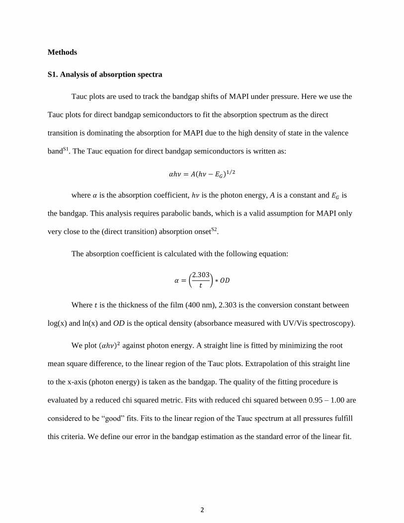
S1. Analysis of absorption spectra

Tauc plots are used to track the bandgap shifts of MAPI under pressure. Here we use the

Tauc plots for direct bandgap semiconductors to fit the absorption spectrum as the direct

transition is dominating the absorption for MAPI due to the high density of state in the valence

bandS1. The Tauc equation for direct bandgap semiconductors is written as:

𝛼ℎ𝜈 = 𝐴(ℎ𝜈 − 𝐸𝐺)1 2⁄

where 𝛼 is the absorption coefficient, ℎ𝜈 is the photon energy, A is a constant and 𝐸𝐺 is

the bandgap. This analysis requires parabolic bands, which is a valid assumption for MAPI only

very close to the (direct transition) absorption onsetS2.

The absorption coefficient is calculated with the following equation:

𝛼 = (2.303

𝑡) ∗ 𝑂𝐷

Where 𝑡 is the thickness of the film (400 nm), 2.303 is the conversion constant between

log(x) and ln(x) and OD is the optical density (absorbance measured with UV/Vis spectroscopy).

We plot (𝛼ℎ𝜈)2 against photon energy. A straight line is fitted by minimizing the root

mean square difference, to the linear region of the Tauc plots. Extrapolation of this straight line

to the x-axis (photon energy) is taken as the bandgap. The quality of the fitting procedure is

evaluated by a reduced chi squared metric. Fits with reduced chi squared between 0.95 – 1.00 are

considered to be “good” fits. Fits to the linear region of the Tauc spectrum at all pressures fulfill

this criteria. We define our error in the bandgap estimation as the standard error of the linear fit.

3

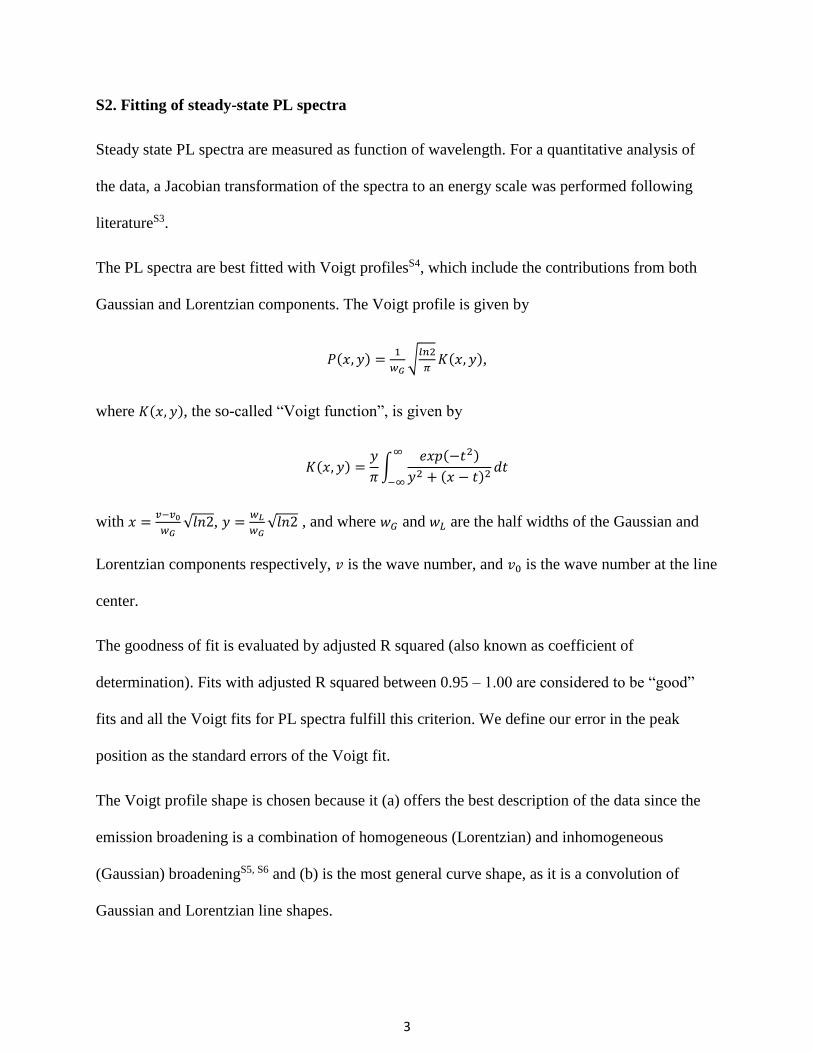
S2. Fitting of steady-state PL spectra

Steady state PL spectra are measured as function of wavelength. For a quantitative analysis of

the data, a Jacobian transformation of the spectra to an energy scale was performed following

literatureS3.

The PL spectra are best fitted with Voigt profilesS4, which include the contributions from both

Gaussian and Lorentzian components. The Voigt profile is given by

𝑃(𝑥, 𝑦) =1

𝑤𝐺√

𝑙𝑛2

𝜋𝐾(𝑥, 𝑦),

where 𝐾(𝑥, 𝑦), the so-called “Voigt function”, is given by

𝐾(𝑥, 𝑦) =𝑦

𝜋∫

𝑒𝑥𝑝(−𝑡2)

𝑦2 + (𝑥 − 𝑡)2𝑑𝑡

∞

−∞

with 𝑥 =𝑣−𝑣0

𝑤𝐺√𝑙𝑛2, 𝑦 =

𝑤𝐿

𝑤𝐺√𝑙𝑛2 , and where 𝑤𝐺 and 𝑤𝐿 are the half widths of the Gaussian and

Lorentzian components respectively, 𝑣 is the wave number, and 𝑣0 is the wave number at the line

center.

The goodness of fit is evaluated by adjusted R squared (also known as coefficient of

determination). Fits with adjusted R squared between 0.95 – 1.00 are considered to be “good”

fits and all the Voigt fits for PL spectra fulfill this criterion. We define our error in the peak

position as the standard errors of the Voigt fit.

The Voigt profile shape is chosen because it (a) offers the best description of the data since the

emission broadening is a combination of homogeneous (Lorentzian) and inhomogeneous

(Gaussian) broadeningS5, S6 and (b) is the most general curve shape, as it is a convolution of

Gaussian and Lorentzian line shapes.

4

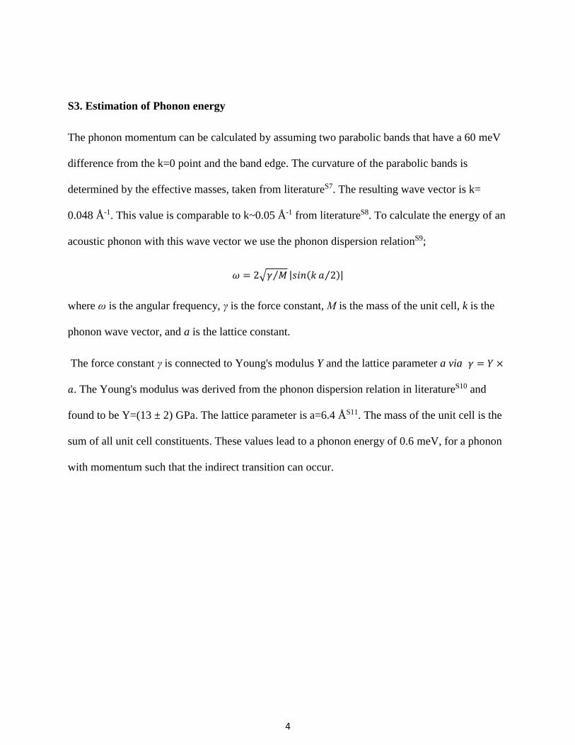
S3. Estimation of Phonon energy

The phonon momentum can be calculated by assuming two parabolic bands that have a 60 meV

difference from the k=0 point and the band edge. The curvature of the parabolic bands is

determined by the effective masses, taken from literatureS7. The resulting wave vector is k=

0.048 Å-1. This value is comparable to k~0.05 Å-1 from literatureS8. To calculate the energy of an

acoustic phonon with this wave vector we use the phonon dispersion relationS9;

𝜔 = 2√𝛾 𝑀⁄ |𝑠𝑖𝑛(𝑘 𝑎 2⁄ )|

where ω is the angular frequency, γ is the force constant, Μ is the mass of the unit cell, k is the

phonon wave vector, and a is the lattice constant.

The force constant γ is connected to Young's modulus Y and the lattice parameter a via 𝛾 = 𝑌 ×

𝑎. The Young's modulus was derived from the phonon dispersion relation in literatureS10 and

found to be Y=(13 ± 2) GPa. The lattice parameter is a=6.4 ÅS11. The mass of the unit cell is the

sum of all unit cell constituents. These values lead to a phonon energy of 0.6 meV, for a phonon

with momentum such that the indirect transition can occur.

5

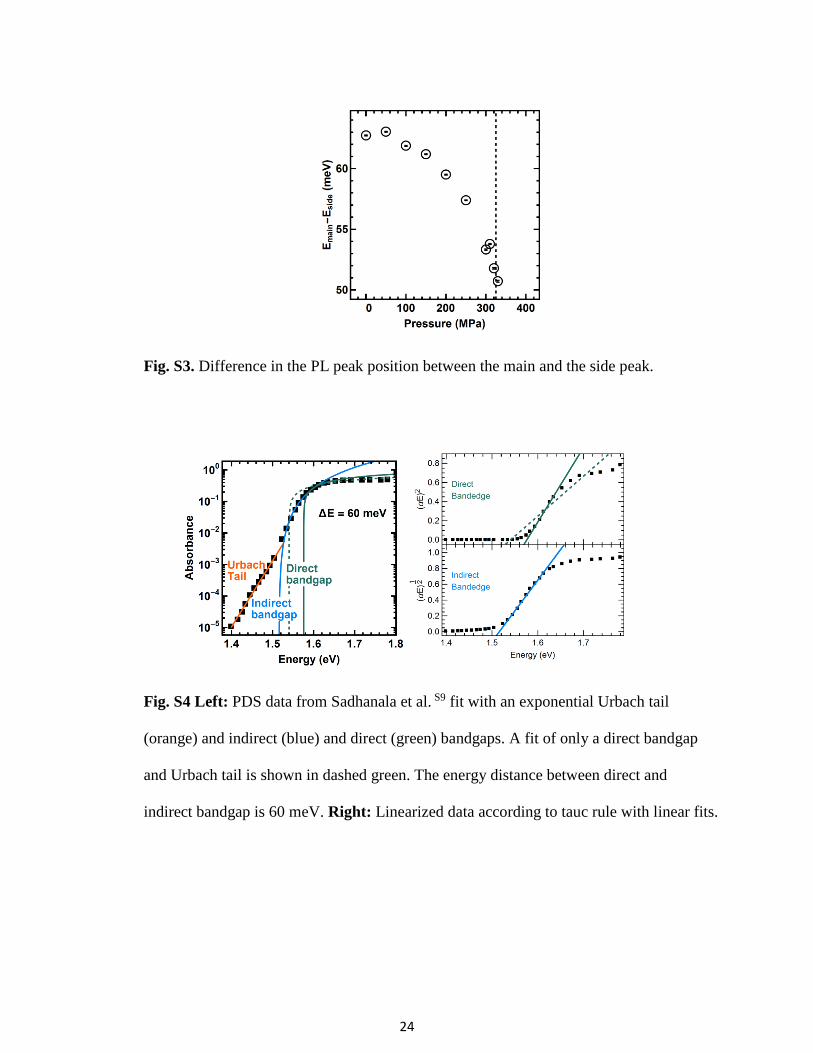
S4. Fit of photothermal deflection spectroscopy (PDS) data

To fit the photothermal deflection spectroscopy data, we use equations for the direct

bandgap, the indirect bandgap, and the Urbach tail. We extracted the absorption data for MAPI

from ref. S12 (Sadhanala et al.) using the website (http://arohatgi.info/WebPlotDigitizer/) (Fig.

S4). As above, the data was then linearized according to the Tauc rule for both direct and indirect

bandgaps:

𝛼ℎ𝜈 = 𝐴(ℎ𝜈 − 𝐸𝐺)𝑟

with the absorption coefficient α, photon energy ℎ𝜈, the scaling constant A, the bandgap

energy EG and the coefficient r (r = 2 for indirect allowed transition, r = ½ for direct allowed

transition)S13, S14. Then the linear region of the plot is identified and a straight line is fitted (with

Mathematica 10.3.1 using LinearModelFit) (Fig. S4). The beginning of the absorbance can be

fitted separately with an exponential, the Urbach tail, usually assigned to shallow traps and

Gaussian disorderS15. The Urbach energy we extract is 21 meV, comparable to the 15 meV

measured beforeS11, S16.

The dashed lines depict an attempt of fitting the whole bandedge with only a direct bandedge and

an Urbach tail.

The fit with only a direct bandgap does not describe the data well, with non-Gaussian distributed

residuals, which led us to the conclusion that an indirect bandgap is also supported from PDS

absorption data.

Additional PDS data is also reported by Zhang et al.S17(Fig. S5) and de Wolf et al.S16(Fig. S6).

Both datasets are also consistent with an indirect bandgap, with a more dominant Urbach tail in

the de Wolf et al. data (Fig. S6).

6

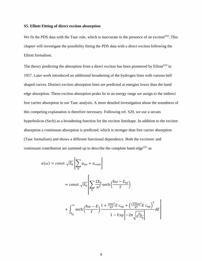
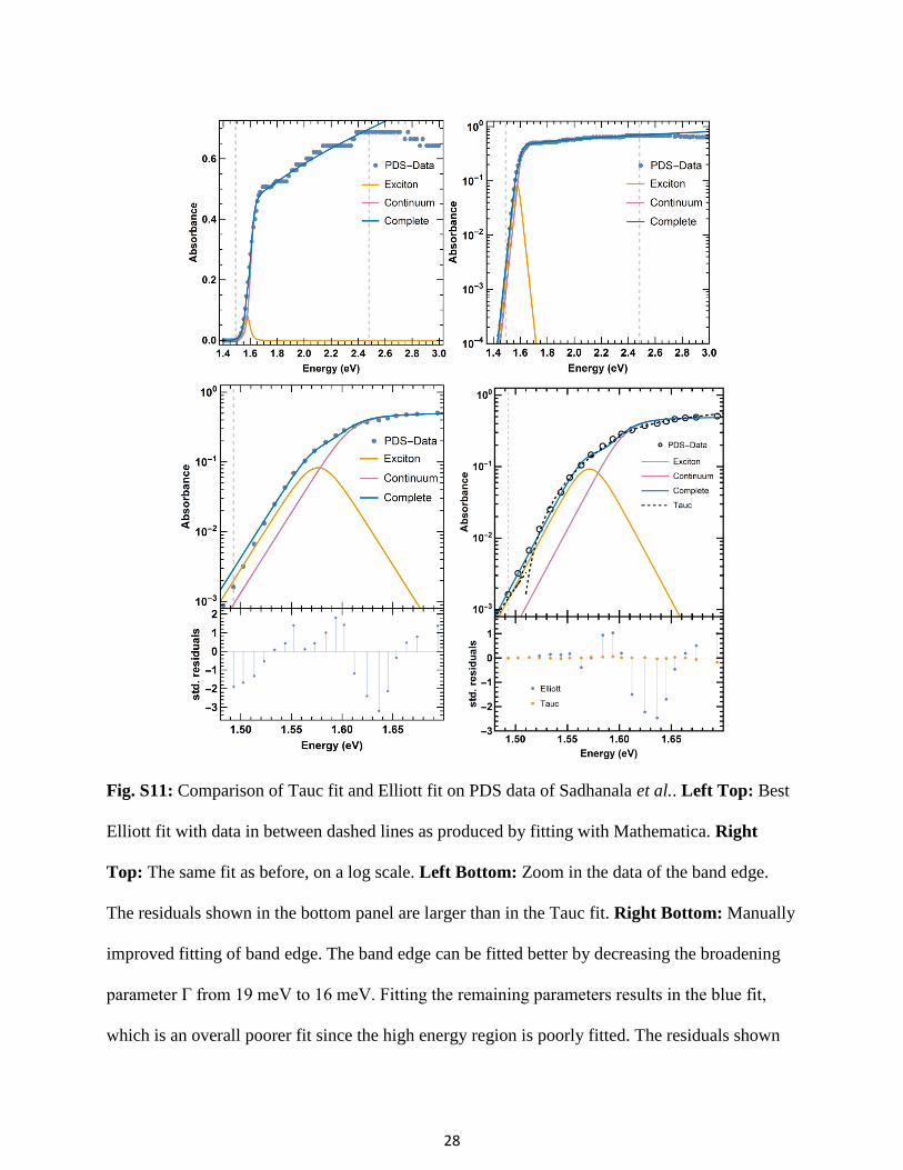
S5. Elliott Fitting of direct exciton absorption

We fit the PDS data with the Tauc rule, which is inaccurate in the presence of an excitonS18. This

chapter will investigate the possibility fitting the PDS data with a direct exciton following the

Elliott formalism.

The theory predicting the absorption from a direct exciton has been pioneered by ElliottS19 in

1957. Later work introduced an additional broadening of the hydrogen lines with various bell

shaped curves. Distinct exciton absorption lines are predicted at energies lower than the band

edge absorption. These exciton absorption peaks lie in an energy range we assign to the indirect

free carrier absorption in our Tauc analysis. A more detailed investigation about the soundness of

this competing explanation is therefore necessary. Following ref. S20, we use a secans

hyperbolicus (Sech) as a broadening function for the exciton lineshape. In addition to the exciton

absorption a continuum absorption is predicted, which is stronger than free carrier absorption

(Tauc formalism) and shows a different functional dependence. Both the excitonic and

continuum contribution are summed up to describe the complete band edgeS21 as

𝛼(𝜔) = 𝑐𝑜𝑛𝑠𝑡. √𝐸𝑏 [∑𝛼𝑛𝑥

𝑛

+ 𝑎𝑐𝑜𝑛𝑡]

= 𝑐𝑜𝑛𝑠𝑡. √𝐸𝑏

[

∑2𝐸𝑏

𝑛3sech (

ℏ𝜔 − 𝐸𝑛𝑥

Γ)

𝑛

+ ∫ sech (ℏ𝜔 − 𝐸

Γ)1 + 10𝑚2

ℏ4 𝐸 𝑐𝑛𝑝 + (√126𝑚2

ℏ4 𝐸 𝑐𝑛𝑝)2

1 − Exp [−2𝜋√𝐸𝑏

𝐸−𝐸𝑔]

d𝐸∞

𝐸𝑔

]

7

where 𝛼 is the absorbance, ω the angular frequency of the absorbed light, const. is a constant

containing the transition dipole moment, 𝐸𝑏 the exciton binding energy, 𝑛 the order of exciton

state, αnx is the absorption from the n-th exction state, αcont is the absorption from the exciton

continuum states, ℏ reduced planc constant, 𝐸𝑛𝑥 = 𝐸𝑔 − (𝐸𝑏/𝑛2) with Eg the bandgap energy,

Γ the line width of the sech function, m the electron mass and E, the energy integral variable. The

integral represents the convolution of the Sech lineshape with the continuum term. The

parameter 𝑐𝑛𝑝 is a correction factor that accounts for a possible deviation from parabolic bands.

The parameter should be small, otherwise the Taylor expansion used in the derivationS22 is no

longer valid. Sestu et al.S20 reports a value of 0.1 eV-1 for 𝑚2

ℏ4 𝑐𝑛𝑝.

We perform a fit on the PDS data reported by Sadhanala et al.S12. In order to fit the absorption

edge the weights are chosen as 1/α. We describe the exponential onset of the absorption data

with the exponential Urbach tail (See Fig. S11) instead of the Elliott fit. In the high energy range

above 2.5 eV the absorption deviates from the continuum shape, we therefor only fit until 2.5 eV.

The data range used in the fit is indicated by the dashed lines in Fig. S11. The fit is global in the

sense that exciton and continuum absorption function share the values for the binding energies

and the peak broadening. Only the first exciton line is considered, higher order excitons are

already overlapping with the continuum absorption and are also of negligible contribution (𝛼 ∝

𝑛−3). Fig. S11 shows the fit and the constituents of the fit. The fit is describing the data

reasonably well. The values the fit produced for the binding energy are reasonable (26 meV)

especially considering the vast discrepancy of binding energies in literatureS23. The exciton peak

is very broad, with a FWHM of 50meV. The non-parabolic correction parameter 𝑚2

ℏ4 𝑐𝑛𝑝 is

−0.015𝑒𝑉−1 which is one order of magnitude smaller than in reference S20, indicating no

significant deviation from parabolic bands. At the band edge we find a systematic deviation

8

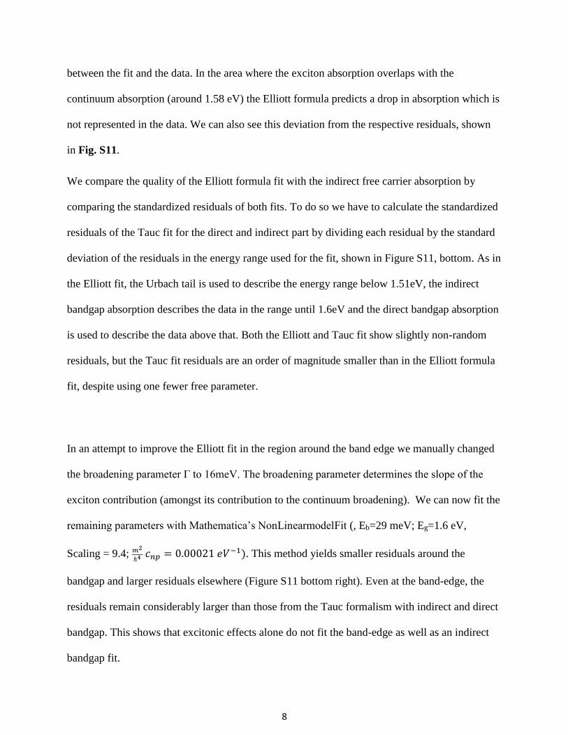
between the fit and the data. In the area where the exciton absorption overlaps with the

continuum absorption (around 1.58 eV) the Elliott formula predicts a drop in absorption which is

not represented in the data. We can also see this deviation from the respective residuals, shown

in Fig. S11.

We compare the quality of the Elliott formula fit with the indirect free carrier absorption by

comparing the standardized residuals of both fits. To do so we have to calculate the standardized

residuals of the Tauc fit for the direct and indirect part by dividing each residual by the standard

deviation of the residuals in the energy range used for the fit, shown in Figure S11, bottom. As in

the Elliott fit, the Urbach tail is used to describe the energy range below 1.51eV, the indirect

bandgap absorption describes the data in the range until 1.6eV and the direct bandgap absorption

is used to describe the data above that. Both the Elliott and Tauc fit show slightly non-random

residuals, but the Tauc fit residuals are an order of magnitude smaller than in the Elliott formula

fit, despite using one fewer free parameter.

In an attempt to improve the Elliott fit in the region around the band edge we manually changed

the broadening parameter Γ to 16meV. The broadening parameter determines the slope of the

exciton contribution (amongst its contribution to the continuum broadening). We can now fit the

remaining parameters with Mathematica’s NonLinearmodelFit (, Eb=29 meV; Eg=1.6 eV,

Scaling = 9.4; 𝑚2

ℏ4 𝑐𝑛𝑝 = 0.00021 𝑒𝑉−1). This method yields smaller residuals around the

bandgap and larger residuals elsewhere (Figure S11 bottom right). Even at the band-edge, the

residuals remain considerably larger than those from the Tauc formalism with indirect and direct

bandgap. This shows that excitonic effects alone do not fit the band-edge as well as an indirect

bandgap fit.

9

We further show that excitonic processes, while present, are insufficient to describe our pressure-

dependent data. We estimate below that the exciton binding energy does not change significantly

over pressure, while the optoelectronic properties of MAPI change dramatically.

We extract the change in exciton binding energy from our UV-Vis absorption measurements.

The data is compatible with no change (see S9 below and Fig. S8, upper bound 26% relative

change), and also shows no change in behavior across the phase transition at 325 MPa. Since

MAPI shows drastic changes in optoelectronic behavior (PLQY, lifetime, bandgap position) over

pressure and across the phase transition, we believe an explanation including excitons alone is

unlikely, contrasted with a straightforward explanation employing the indirect bandgap induced

by Rashba splitting.

S6. Analysis of TCSPC data

First the differential equation relating the decay of charge carrier density and the

bimolecular (assumed radiative) and monomolecular (assumed non-radiative) decay is solved

(see Equation 1 of the main text). This model does not include Auger recombination, since this

contribution is negligible, as shown below. This model assumes that an equal amount of

electrons and holes are generated upon photoexcitation, and that the excitation leads to a much

higher charge carrier density than the intrinsically available charge carrier density. Both

electrons and holes are treated as equivalent charge carriers since in MAPI perovskites mobility

of holes and electrons is comparableS24. We normalize the data at t = 0 and set the boundary

condition for the charge carrier density in the fit accordingly to

𝑛(𝑡 = 0) = 𝑛0 = 1 𝑐⁄ 𝑚3.

10

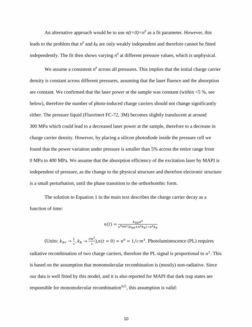
An alternative approach would be to use n(t=0)=n0 as a fit parameter. However, this

leads to the problem that n0 and kR are only weakly independent and therefore cannot be fitted

independently. The fit then shows varying n0 at different pressure values, which is unphysical.

We assume a consistent n0 across all pressures. This implies that the initial charge carrier

density is constant across different pressures, assuming that the laser fluence and the absorption

are constant. We confirmed that the laser power at the sample was constant (within <5 %, see

below), therefore the number of photo-induced charge carriers should not change significantly

either. The pressure liquid (Fluorinert FC-72, 3M) becomes slightly translucent at around

300 MPa which could lead to a decreased laser power at the sample, therefore to a decrease in

charge carrier density. However, by placing a silicon photodiode inside the pressure cell we

found that the power variation under pressure is smaller than 5% across the entire range from

0 MPa to 400 MPa. We assume that the absorption efficiency of the excitation laser by MAPI is

independent of pressure, as the change to the physical structure and therefore electronic structure

is a small perturbation, until the phase transition to the orthorhombic form.

The solution to Equation 1 in the main text describes the charge carrier decay as a

function of time:

𝑛(𝑡) =𝑘𝑁𝑅𝑛0

𝑒𝑘𝑁𝑅𝑡(𝑘𝑁𝑅+𝑛0𝑘𝑅)−𝑛0𝑘𝑅

(Units: 𝑘𝑁𝑟 →1

𝑠, 𝑘𝑅 →

𝑐𝑚3

𝑠),𝑛(𝑡 = 0) = 𝑛0 = 1 𝑐⁄ 𝑚3. Photoluminescence (PL) requires

radiative recombination of two charge carriers, therefore the PL signal is proportional to 𝑛2. This

is based on the assumption that monomolecular recombination is (mostly) non-radiative. Since

our data is well fitted by this model, and it is also reported for MAPI that dark trap states are

responsible for monomolecular recombinationS25, this assumption is valid:

11

𝑃𝑙(𝑡) = 𝐴𝑛(𝑡)2 + 𝑏𝑎𝑐𝑘𝑔𝑟𝑜𝑢𝑛𝑑

The proportionality factor A includes the number of generated photons (dependent on the

charge carrier density n0) and the outcoupling efficiency. The sum of A and the background is

described by the height of the PL decay curve at t = 0 in our model with normalized n0. The

background is determined independently by fitting the average of the datapoints before the

excitation pulse. The Instrument Response Function (IRF) at 640 nm has a FWHM of 1 ns, so to

exclude any effects of the IRF on our analysis we start fitting from 1 ns onwards. Fitting uses the

NonLinearFit function in Mathematica 10.3. This algorithm minimizes the Chi-squared value to

find the best fit while using 1/cts as weighing factor since √𝑐𝑡𝑠 is the error on (Poisson-

distributed) counting data. The Chi-squared method assumes that the datapoints are scattered

around the “real” curve following a normal distribution. As we are counting photons in

photoluminescence measurements, the real scatter histogram follows a Poisson distribution. If

the mean of a Poisson distribution is sufficiently high (conventionally µ > 10) it can be

approximated by a normal distribution. We implement this by fitting the data only until the

intensity has reached background + 15 counts. In this range the residuals should follow the

normal distribution in good approximation. This null hypothesis is then tested with a Cramér-von

Mises test, resulting in a reliable goodness of fit measure for our highly nonlinear model (Chi-

Squared reduced close to 1 should not be used with nonlinear models as shown in literatureS26.

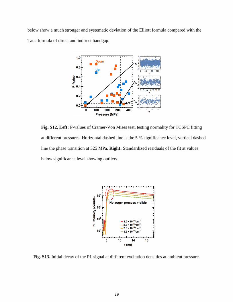
The p-values of the Cramer-Von Mises test are shown in Fig. S12, all but three have a

significance level P > 0.05. Residuals of the three fits with P < 0.05 are included in Fig. S12 and

show no structure but a few outliers producing the low P-Values, hence the fit can also be

accepted in those cases. The results of the fitted parameters can be found in the main text.

We define the radiative efficiency as follows:

12

𝛩𝑅𝑎𝑑 =𝑐ℎ𝑎𝑟𝑔𝑒𝑐𝑎𝑟𝑟𝑖𝑒𝑟𝑠𝑑𝑒𝑐𝑎𝑦𝑒𝑑𝑏𝑖𝑚𝑜𝑙𝑒𝑐𝑢𝑙𝑎𝑟𝑙𝑦

𝑎𝑙𝑙𝑑𝑒𝑐𝑎𝑦𝑒𝑑𝑐ℎ𝑎𝑟𝑔𝑒𝑐𝑎𝑟𝑟𝑖𝑒𝑟𝑠=

∫ 𝑘𝑏𝑖𝑛(𝑡)2𝑑𝑡∞

𝑡=0

∫ [𝑘𝑏𝑖𝑛(𝑡)2 + 𝑘𝑚𝑜𝑛𝑜𝑛(𝑡)]𝑑𝑡∞

𝑡=0

Similarly, the fraction of charge carriers decayed non-radiatively is defined as

𝛩𝑁𝑜𝑛𝑅𝑎𝑑 =∫ 𝑘𝑚𝑜𝑛𝑜𝑛(𝑡)𝑑𝑡

∞

𝑡=0

∫ [𝑘𝑏𝑖𝑛(𝑡)2 + 𝑘𝑏𝑖𝑛(𝑡)]𝑑𝑡∞

𝑡=0

while 𝛩𝑁𝑜𝑛𝑅𝑎𝑑 + 𝛩𝑅𝑎𝑑 = 1. Both values are plotted in Fig. 2C of the main text.

On Auger recombination: To determine the influence of Auger recombination (∝ 𝑛3)

and to show that the two-process model used here is sufficient, we carried out TCSPC

measurements at different excitation densities. At 0 MPa, we varied the laser power by one order

of magnitude compared to the other measurements. Since Auger recombination is a fast process

it would be visible in the onset of the decay, rising with the cube of the excitation density. As

seen in Fig. S13, no evidence is shown for Auger recombination in our TCSPC measurements.

Influence of charge carrier density: The increased radiative efficiency we observe could

also arise through higher charge carrier densities, as discussed in literatureS27, S28 and from the

dependence of ΘRad which increases with charge carrier density. The laser power was held

constant (variation <5%, photodiode measurement, see above) during the measurement and the

sample was fixed in a sample holder, restricting movement and therefore fixing the incoming

laser power density. To show that even large variations in charge carrier densities do not lead to

our observed simultaneous increase in kmono and kbi we fitted the TCSPC data where we changed

the laser intensity with the model assuming constant laser power. This shows an increase in kbi

(Fig. S14) but a stable kmono (Fig. S15) with increasing laser power, different from the trend in

the pressure TCSPC experiment. The apparent increase in kbi extracted from the fit is due to the

fast radiative component becoming more important with higher charge carrier density and the

13

model can only increase the value of kbi to optimize the fit when the amplitude is fixed. A

decrease in charge carrier density over pressure would lead to a decrease in radiative efficiency,

opposite to the trend of increasing radiative efficiency in the pressure measurement. If we take

the model with varying initial charge carrier density and fit the data with n0 as the only fitting

parameter, (holding kmono and kbi constant), we are able to fit the data taken at different excitation

densities (Fig. S16).

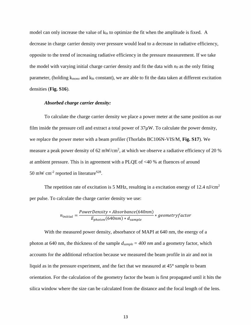
Absorbed charge carrier density:

To calculate the charge carrier density we place a power meter at the same position as our

film inside the pressure cell and extract a total power of 37µW. To calculate the power density,

we replace the power meter with a beam profiler (Thorlabs BC106N-VIS/M, Fig. S17). We

measure a peak power density of 62 mW/cm2, at which we observe a radiative efficiency of 20 %

at ambient pressure. This is in agreement with a PLQE of <40 % at fluences of around

50 mW cm-2 reported in literatureS28.

The repetition rate of excitation is 5 MHz, resulting in a excitation energy of 12.4 nJ/cm2

per pulse. To calculate the charge carrier density we use:

𝑛𝑖𝑛𝑖𝑡𝑖𝑎𝑙 =𝑃𝑜𝑤𝑒𝑟𝐷𝑒𝑛𝑠𝑖𝑡𝑦 ∗ 𝐴𝑏𝑠𝑜𝑟𝑏𝑎𝑛𝑐𝑒(640𝑛𝑚)

𝐸𝑝ℎ𝑜𝑡𝑜𝑛(640𝑛𝑚) ∗ 𝑑𝑠𝑎𝑚𝑝𝑙𝑒∗ 𝑔𝑒𝑜𝑚𝑒𝑡𝑟𝑦𝑓𝑎𝑐𝑡𝑜𝑟

With the measured power density, absorbance of MAPI at 640 nm, the energy of a

photon at 640 nm, the thickness of the sample dsample = 400 nm and a geometry factor, which

accounts for the additional refraction because we measured the beam profile in air and not in

liquid as in the pressure experiment, and the fact that we measured at 45° sample to beam

orientation. For the calculation of the geometry factor the beam is first propagated until it hits the

silica window where the size can be calculated from the distance and the focal length of the lens.

14

The beam is then refracted twice, once at the air-silica and then at the silica-liquid interface. The

beam is then propagated to the sample, where the beam radius is calculated again. This results in

a ratio of the squares of these radii of 2.14. In addition, the sample is tilted by 45° from the

incoming beam during the pressure measurement, so we add a factor of cos(45°) resulting in a

total geometry factor of 1.51.

This leads to an initial charge carrier density of 6.05×1014 cm-3.

Comparison with literature values for the rate constants: Wehrenfennig et al. carried

out a measurement of the rate constants at ambient pressure on films of the same material using

THz techniquesS28. We compare this with our measurement at 0 MPa. Wehrenfennig et al.

measured at charge carrier densities of 1017-1019 cm-3, considerably higher than our density of

1014 cm-3. They report a non-radiative recombination rate of 14 µs-1, whereas we measure

(20.0 ± 0.2) µs-1, with the error derived from the fit. They report a radiative recombination rate of

kbilit. = 9.2 × 10-10 cm3 s-1. Our calculation is using an initial charge carrier density of unity (1 cm-

3). Therefore 𝑘𝑏𝑖𝑅𝑒𝑎𝑙 =

𝑘𝑏𝑖𝑓𝑖𝑡

𝑛(𝑡=0), here (1.85 ± 0.05) × 10-8 cm3 s-1, around 20 times higher than

reported by Wehrenfennig et al. The vastly different excitation densitiesS8 as well as the different

techniques (TCSPC vs. THz photoconductivity measurements) and batch-to-batch variations

might explain the difference.

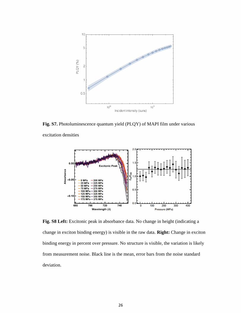
S7. Determination of PLQY

We used an integrating sphere setup to estimate the photoluminescence quantum yield of the

identical MAPI film used in the main text. We determine the absorbed power and the

luminescence directly, by using a photodetector combined with a long-pass filter (for

15

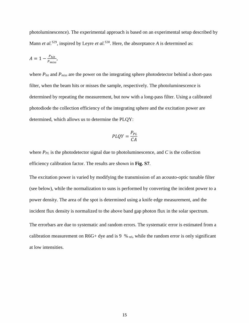
photoluminescence). The experimental approach is based on an experimental setup described by

Mann et al.S29, inspired by Leyre et al.S30. Here, the absorptance A is determined as:

𝐴 = 1 −𝑃ℎ𝑖𝑡

𝑃𝑚𝑖𝑠𝑠,

where Phit and Pmiss are the power on the integrating sphere photodetector behind a short-pass

filter, when the beam hits or misses the sample, respectively. The photoluminescence is

determined by repeating the measurement, but now with a long-pass filter. Using a calibrated

photodiode the collection efficiency of the integrating sphere and the excitation power are

determined, which allows us to determine the PLQY:

𝑃𝐿𝑄𝑌 =𝑃𝑃𝐿

𝐶𝐴

where PPL is the photodetector signal due to photoluminescence, and C is the collection

efficiency calibration factor. The results are shown in Fig. S7.

The excitation power is varied by modifying the transmission of an acousto-optic tunable filter

(see below), while the normalization to suns is performed by converting the incident power to a

power density. The area of the spot is determined using a knife edge measurement, and the

incident flux density is normalized to the above band gap photon flux in the solar spectrum.

The errorbars are due to systematic and random errors. The systematic error is estimated from a

calibration measurement on R6G+ dye and is 9 % rel, while the random error is only significant

at low intensities.

16

S8. Different methods for MAPI thin film preparation and their corresponding PL spectra

To investigate the influence of trap states, impurities, and morphological changes induced by

different sample preparation methods, we prepared MAPbI3 thin films with various methods,

namely spincoating with and without antisolvent precipitation, solution casting, and two-step

dipping (lead iodide (PbI2) used as lead precursor for all methods mentioned above) and

spincoating using lead acetate (PbAc2) as lead precursor. All operations were performed in a

nitrogen-filled glovebox unless specified. All PL measurements were performed under the same

experimental condition as described in the main text unless mentioned specifically.

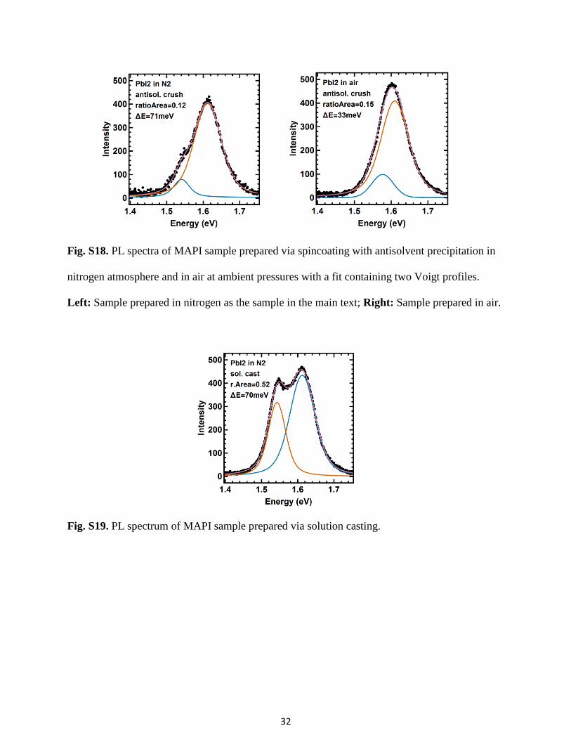
For spincoating with antisolvent precipitation, the procedure was described in the Methods

section of the main text. We repeat the preparation method described in the main text to estimate

the sample-to-sample variation. Additionally, we prepare the same sample in air without

changing other parameters. The sample prepared in nitrogen atmosphere shows a PL spectrum

with a clear side peak (see Fig. S18), which is comparable to the PL spectrum shown in the main

text. The sample prepared in air also shows the sidepeak PL spectrum, yet with lower intensity

(see Fig. S18).

For solution casting, 100 µL of hot (100 ºC) MAPI solution (37 %, wt.) in DMF with a molar

ratio of 1:1 between PbI2 and MAI was deposited on top of fused silica substrate that was placed

on a hotplate at 100 ºC under nitrogen atmosphere for 30 min. The PL spectrum of solution-cast

sample is shown in Fig. S19, where a clear side peak is also visible.

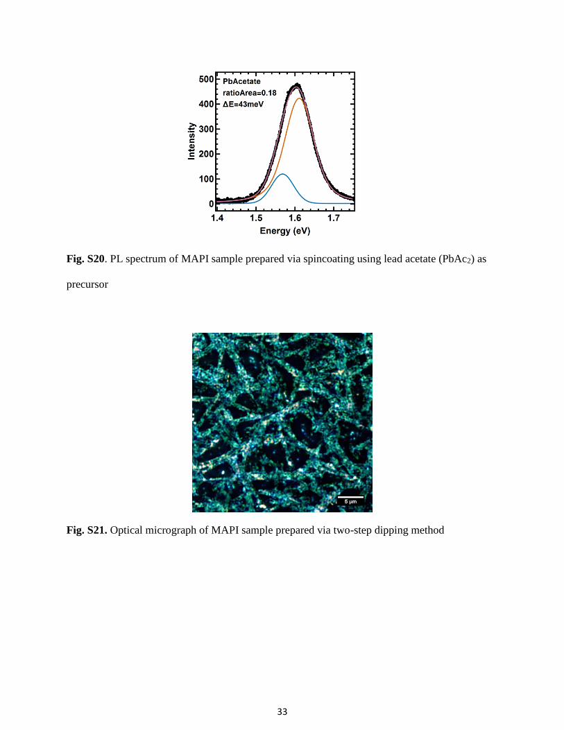
For using PbAc2 as lead precursor, PbAc2 and methylammonium iodide (MAI) were dissolved in

DMF with a molar ratio of 1:3 at 100 °C to obtain a 1M solution of MAPI. The solution was then

spincoated onto fused silica substrates at 2000 rpm for 45 seconds. Then the sample is left to dry

at room temperature for 10 min. The dried sample was transferred to a hotplate and annealed at

17

100 °C for 10 min. The sample prepared with PbAc2 also shows an asymmetric PL spectrum (see

Fig. S20) and two peaks are needed for a good fit of the spectrum.

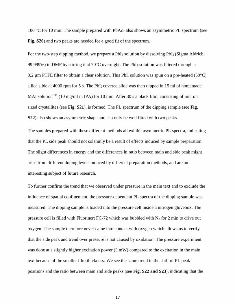
For the two-step dipping method, we prepare a PbI2 solution by dissolving PbI2 (Sigma Aldrich,

99.999%) in DMF by stirring it at 70°C overnight. The PbI2 solution was filtered through a

0.2 µm PTFE filter to obtain a clear solution. This PbI2 solution was spun on a pre-heated (50°C)

silica slide at 4000 rpm for 5 s. The PbI2 covered slide was then dipped in 15 ml of homemade

MAI solutionS31 (10 mg/ml in IPA) for 10 min. After 30 s a black film, consisting of micron

sized crystallites (see Fig. S21), is formed. The PL spectrum of the dipping sample (see Fig.

S22) also shows an asymmetric shape and can only be well fitted with two peaks.

The samples prepared with these different methods all exhibit asymmetric PL spectra, indicating

that the PL side peak should not solemnly be a result of effects induced by sample preparation.

The slight differences in energy and the differences in ratio between main and side peak might

arise from different doping levels induced by different preparation methods, and are an

interesting subject of future research.

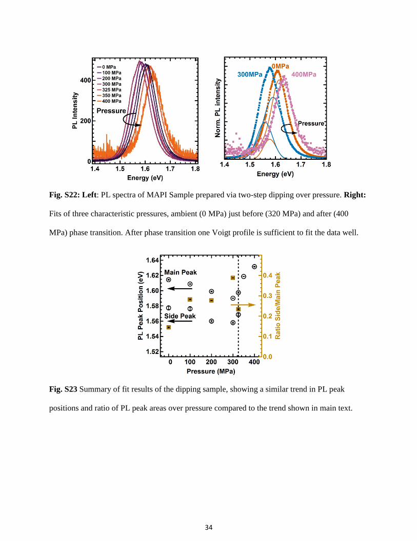
To further confirm the trend that we observed under pressure in the main text and to exclude the

influence of spatial confinement, the pressure-dependent PL spectra of the dipping sample was

measured. The dipping sample is loaded into the pressure cell inside a nitrogen glovebox. The

pressure cell is filled with Fluorinert FC-72 which was bubbled with N2 for 2 min to drive out

oxygen. The sample therefore never came into contact with oxygen which allows us to verify

that the side peak and trend over pressure is not caused by oxidation. The pressure experiment

was done at a slightly higher excitation power (3 mW) compared to the excitation in the main

text because of the smaller film thickness. We see the same trend in the shift of PL peak

positions and the ratio between main and side peaks (see Fig. S22 and S23), indicating that the

18

effect that we observe is not sensitive to spatial confinement, oxygen, and is reproducible for a

sample prepared by a different method.

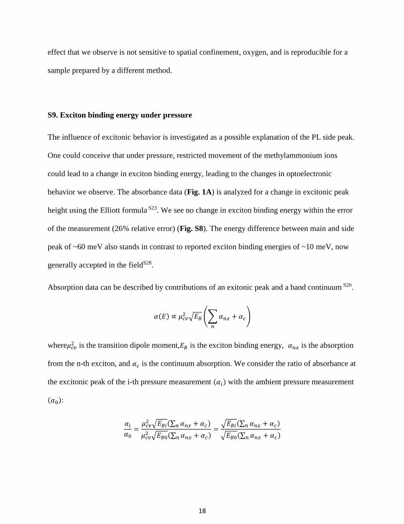
S9. Exciton binding energy under pressure

The influence of excitonic behavior is investigated as a possible explanation of the PL side peak.

One could conceive that under pressure, restricted movement of the methylammonium ions

could lead to a change in exciton binding energy, leading to the changes in optoelectronic

behavior we observe. The absorbance data (Fig. 1A) is analyzed for a change in excitonic peak

height using the Elliott formula S23. We see no change in exciton binding energy within the error

of the measurement (26% relative error) (Fig. S8). The energy difference between main and side

peak of ~60 meV also stands in contrast to reported exciton binding energies of ~10 meV, now

generally accepted in the fieldS28.

Absorption data can be described by contributions of an exitonic peak and a band continuum S20.

𝛼(𝐸) ∝ 𝜇𝑐𝑣2 √𝐸𝐵 (∑𝛼𝑛𝑥 + 𝛼𝑐

𝑛

)

where𝜇𝑐𝑣2 is the transition dipole moment,𝐸𝐵 is the exciton binding energy, 𝛼𝑛𝑥 is the absorption

from the n-th exciton, and 𝛼𝑐 is the continuum absorption. We consider the ratio of absorbance at

the excitonic peak of the i-th pressure measurement (𝛼𝑖) with the ambient pressure measurement

(𝛼0):

𝛼𝑖

𝛼0=

𝜇𝑐𝑣2 √𝐸𝐵𝑖(∑ 𝛼𝑛𝑥 + 𝛼𝑐𝑛 )

𝜇𝑐𝑣2 √𝐸𝐵0(∑ 𝛼𝑛𝑥 + 𝛼𝑐𝑛 )

=√𝐸𝐵𝑖(∑ 𝛼𝑛𝑥 + 𝛼𝑐𝑛 )

√𝐸𝐵0(∑ 𝛼𝑛𝑥 + 𝛼𝑐𝑛 )

19

To calculate an upper bound of change in exciton binding energy we assume a strong continuum

contribution, and consider the limit of 𝛼𝑐 → ∞. This limit leads to:

𝛼𝑖

𝛼0=

√𝐸𝐵𝑖

√𝐸𝐵0

⇒𝐸𝐵𝑖

𝐸𝐵0= (

𝛼𝑖

𝛼0)2

To get the value of 𝛼𝑖

𝛼0, we determine the maxima of the excitonic peak. To show the excitonic

peak more clearly than in Fig. 1A we treat the data. We fit a linear equation to the low

wavelength realm in the data of Fig. 1A for every curve and subtract the respective line from the

data (Fig. S8)

We use the function Lowpass in Mathematica 10.3 to filter the noise and extract the maximum

peak value for each pressure point seen in Fig. S8. We then calculate the change in exciton

binding energy from the peak absorbance data points (Fig. S8). The upper bound for the increase

in exciton binding energy is 26% with a large standard deviation of 11% also represented in the

large error bars. Error bars are taken from the standard deviation of the noise, propagated via a

Gaussian error propagation according to the formula above.

20

References

S1. J. Tauc, Materials Research Bulletin, 1968, 3, 37-46.

S2. F. Brivio, K. T. Butler, A. Walsh and M. van Schilfgaarde, Physical Review B, 2014, 89.

S3. J. Mooney and P. Kambhampati, The Journal of Physical Chemistry Letters, 2013, 4,

3316-3318.

S4. B. H. Armstrong, Journal of Quantitative Spectroscopy and Radiative Transfer, 1967, 7,

61-88.

S5. A. D. Wright, C. Verdi, R. L. Milot, G. E. Eperon, M. A. Pérez-Osorio, H. J. Snaith, F.

Giustino, M. B. Johnston and L. M. Herz, Nature Communications, 2016, 7, 0.

S6. C. Wehrenfennig, M. Liu, H. J. Snaith, M. B. Johnston and L. M. Herz, The Journal of

Physical Chemistry Letters, 2014, 5, 1300-1306.

S7. J. M. Frost, K. T. Butler, F. Brivio, C. H. Hendon, M. van Schilfgaarde and A. Walsh,

Nano Letters, 2014, 14, 2584-2590.

S8. P. Azarhoosh, S. McKechnie, J. M. Frost, A. Walsh and M. van Schilfgaarde, APL

Materials, 2016, 4, 091501.

S9. C. Kittel, Introduction to Solid State Physics. John Wiley and Sons, Inc., New York, 8th

edition, 2005.

S10. Beecher, A. N. et al. The cubic phase of methylammonium lead iodide perovskite is not

locally cubic. 1–10 (2016).

S11. Oku, T. Sol. Cells - New Approaches Rev. 2015, 77–101. doi:10.5772/58490

21

S12. A. Sadhanala, F. Deschler, T. H. Thomas, S. E. Dutton, K. C. Goedel, F. C. Hanusch, M.

L. Lai, U. Steiner, T. Bein, P. Docampo, D. Cahen and R. H. Friend, Journal of Physical

Chemistry Letters, 2014, 5, 2501-2505.

S13. J. Tauc, R. Grigorovici and A. Vancu, physica status solidi (b), 1966, 15, 627-637.

S14. E. A. Davis and N. F. Mott, Philosophical Magazine, 1970, 22, 0903-0922.

S15. S. John, C. Soukoulis, M. H. Cohen and E. N. Economou, Physical Review Letters, 1986,

57, 1777-1780.

S16. S. De Wolf, J. Holovsky, S. J. Moon, P. Loper, B. Niesen, M. Ledinsky, F. J. Haug, J. H.

Yum and C. Ballif, The Journal of Physical Chemistry Letters, 2014, 5, 1035-1039.

S17. W. Zhang, M. Saliba, D. T. Moore, S. K. Pathak, M. T. Horantner, T. Stergiopoulos, S.

D. Stranks, G. E. Eperon, J. A. Alexander-Webber, A. Abate, A. Sadhanala, S. Yao, Y. Chen, R.

H. Friend, L. A. Estroff, U. Wiesner and H. J. Snaith, Nature Communications, 2015, 6, 6142.

S18. M. A. Green, Y. J. Jiang, A. M. Soufiani and A. Ho-Baillie, Journal of Physical

Chemistry Letters, 2015, 6, 4774-4785

S19. R. J. Elliott, Physical Review, 1957, 108, 1384-1389

S20. N. Sestu, M. Cadelano, V. Sarritzu, F. Chen, D. Marongiu, R. Piras, M. Mainas, F.

Quochi, M. Saba, A. Mura and G. Bongiovanni, The Journal of Physical Chemistry Letters,

2015, 6, 4566-4572.

S21. R. G. Glinskt, K. S. Song and J. C. Woolley, Physica Status Solidi (b), 1971, 48, 815-822.

S22. M. Cadelano, PhD thesis, UNIVERSITÀ DEGLI STUDI DI CAGLIARI, 2016.

S23. L. M. Herz, Annual Reviews of Physical Chemistry, 2016, 67, 65-89.

22

S24. C. Motta, F. El-Mellouhi and S. Sanvito, Scientific Reports, 2015, 5, 12746.

S25. G.-J. A. H. Wetzelaer, M. Scheepers, A. M. Sempere, C. Momblona, J. Ávila and H. J.

Bolink, Advanced Materials, 2015, 27, 1837-1841.

S26. R. Andrae, T. Schulze-Hartung, P. Melchior, Dos and don'ts of reduced chi-squared,

2010, arXiv:1012.3754v1

S27. F. Deschler, M. Price, S. Pathak, L. E. Klintberg, D. D. Jarausch, R. Higler, S. Huttner, T.

Leijtens, S. D. Stranks, H. J. Snaith, M. Atature, R. T. Phillips and R. H. Friend, The Journal of

Physical Chemistry Letters, 2014, 5, 1421-1426.

S28. C. Wehrenfennig, G. E. Eperon, M. B. Johnston, H. J. Snaith and L. M. Herz, Advanced

Materials, 2014, 26, 1584-1589.

S29. S. A. Mann, S. Z. Oener, A. Cavalli, J. E. M. Haverkort, E. P. A. M. Bakkers and E. C.

Garnett, Nature Nanotechnology, 2016, advance online publication.

S30. S. Leyre, E. Coutino-Gonzalez, J. J. Joos, J. Ryckaert, Y. Meuret, D. Poelman, P. F. Smet,

G. Durinck, J. Hofkens, G. Deconinck and P. Hanselaer, Review of Scientific Instruments, 2014,

85, 123115.

S31. G. W. P. Adhyaksa, L. W. Veldhuizen, Y. Kuang, S. Brittman, R. E. I. Schropp and E. C.

Garnett, Chemistry of Materials, 2016, 28, 5259-5263.

23

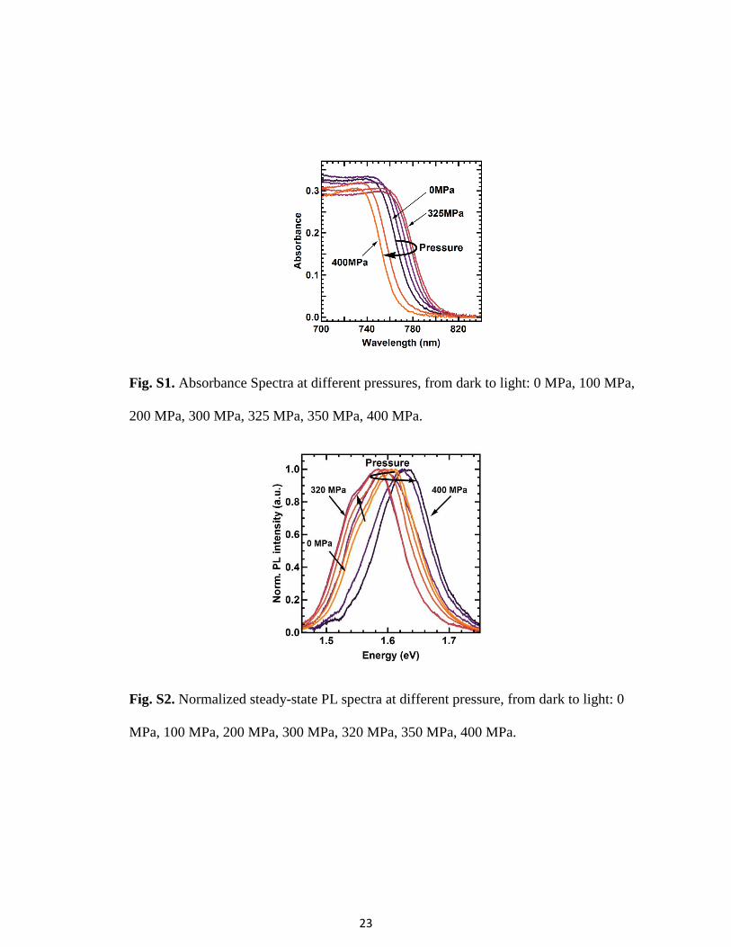
Fig. S1. Absorbance Spectra at different pressures, from dark to light: 0 MPa, 100 MPa,

200 MPa, 300 MPa, 325 MPa, 350 MPa, 400 MPa.

Fig. S2. Normalized steady-state PL spectra at different pressure, from dark to light: 0

MPa, 100 MPa, 200 MPa, 300 MPa, 320 MPa, 350 MPa, 400 MPa.

24

Fig. S3. Difference in the PL peak position between the main and the side peak.

Fig. S4 Left: PDS data from Sadhanala et al. S9 fit with an exponential Urbach tail

(orange) and indirect (blue) and direct (green) bandgaps. A fit of only a direct bandgap

and Urbach tail is shown in dashed green. The energy distance between direct and

indirect bandgap is 60 meV. Right: Linearized data according to tauc rule with linear fits.

25

Fig. S5 Left: PDS data from de Wolf et al. S13 fit with an exponential Urbach tail

(orange) and indirect (blue) and direct (green) bandgaps. A fit of only a direct bandgap

and Urbach tail is shown in dashed green. The energy distance between direct and

indirect bandgap is 46 meV. A large Urbach tail overlaps with the indirect bandgap.

Right: Linearized data according to tauc rule with linear fits.

Fig. S6 Left: PDS data from Zhang et al. S14 fit with an exponential Urbach tail (orange)

and indirect (blue) and direct (green) bandgaps. A fit of only a direct bandgap and Urbach

tail is shown in dashed green. The energy distance between direct and indirect bandgap is

53 meV. Right: Linearized data according to tauc rule with linear fits.

26

Fig. S7. Photoluminescence quantum yield (PLQY) of MAPI film under various

excitation densities

Fig. S8 Left: Excitonic peak in absorbance data. No change in height (indicating a

change in exciton binding energy) is visible in the raw data. Right: Change in exciton

binding energy in percent over pressure. No structure is visible, the variation is likely

from measurement noise. Black line is the mean, error bars from the noise standard

deviation.

27

Fig. S9. Scanning electron micrograph of MAPI thin film on quartz substrate.

Fig. S10. Absorption spectra with transparent and translucent pressure liquid. The inset

shows the normalized absorption spectra of the pressure liquid without sample at elevated

pressure. The spectral response is flat around the band-edge.

28

Fig. S11: Comparison of Tauc fit and Elliott fit on PDS data of Sadhanala et al.. Left Top: Best

Elliott fit with data in between dashed lines as produced by fitting with Mathematica. Right

Top: The same fit as before, on a log scale. Left Bottom: Zoom in the data of the band edge.

The residuals shown in the bottom panel are larger than in the Tauc fit. Right Bottom: Manually

improved fitting of band edge. The band edge can be fitted better by decreasing the broadening

parameter Γ from 19 meV to 16 meV. Fitting the remaining parameters results in the blue fit,

which is an overall poorer fit since the high energy region is poorly fitted. The residuals shown

29

below show a much stronger and systematic deviation of the Elliott formula compared with the

Tauc formula of direct and indirect bandgap.

Fig. S12. Left: P-values of Cramer-Von Mises test, testing normality for TCSPC fitting

at different pressures. Horizontal dashed line is the 5 % significance level, vertical dashed

line the phase transition at 325 MPa. Right: Standardized residuals of the fit at values

below significance level showing outliers.

Fig. S13. Initial decay of the PL signal at different excitation densities at ambient pressure.

30

Fig. S14. Data seen in Fig. S13 fitted to our model forcing constant charge carrier

density. Because the actual charge carrier density varies, the model has to increase the

bimolecular rate to account for a faster onset of decay.

Fig. S15. Data seen in Fig. S13 fitted to our model forcing constant charge carrier

density. The monomolecular rate stays largely unaffected by the change in charge carrier

density.

31

Fig. S16. Data shown in Fig. S4 fitted globally while allowing for varying charge carrier

density. Both monomolecular and bimolecular rates are fixed to the rates retrieved under

ambient pressure. The faster decay onset is reproduced correctly by an increase in charge

carrier density.

Fig. S17. Beam profile measured in air with the same lens and the same lens to sample

distance as in the pressure experiment.

32

Fig. S18. PL spectra of MAPI sample prepared via spincoating with antisolvent precipitation in

nitrogen atmosphere and in air at ambient pressures with a fit containing two Voigt profiles.

Left: Sample prepared in nitrogen as the sample in the main text; Right: Sample prepared in air.

Fig. S19. PL spectrum of MAPI sample prepared via solution casting.

33

Fig. S20. PL spectrum of MAPI sample prepared via spincoating using lead acetate (PbAc2) as

precursor

Fig. S21. Optical micrograph of MAPI sample prepared via two-step dipping method

34

Fig. S22: Left: PL spectra of MAPI Sample prepared via two-step dipping over pressure. Right:

Fits of three characteristic pressures, ambient (0 MPa) just before (320 MPa) and after (400

MPa) phase transition. After phase transition one Voigt profile is sufficient to fit the data well.

Fig. S23 Summary of fit results of the dipping sample, showing a similar trend in PL peak

positions and ratio of PL peak areas over pressure compared to the trend shown in main text.