Embed Size (px)
Citation preview

Independent dose CalCulatIons ConCepts and Models

2010-First edition ISBN 90-804532-9©2010 by ESTRO
All rights reservedNo part of this publication may be reproduced,
stored in a retrieval system, or transmitted in any form or by any means, electronic, mechanical, photocopying, recording or otherwise
without the prior permission of the copyright owners.
ESTROMounierlaan 83/12 – 1200 Brussels (Belgium)

III
authors:
Mikael Karlsson, Department of Radiation Sciences, University Hospital of Northern Swe-den, Umeå, Sweden.
Anders Ahnesjö, Department of Oncology, Radiology and Clinical Immunology, Uppsala University, Akademiska Sjukhuset, Uppsala, Sweden and Nucletron AB, Uppsala, Sweden.
Dietmar Georg, Division Medical Radiation Physics, Department of Radiotherapy, Medical University Vienna/AKH, Wien, Austria.
Tufve Nyholm, Department of Radiation Sciences, University Hospital of Northern Sweden, Umeå, Sweden.
Jörgen Olofsson, Department of Radiation Sciences, University Hospital of Northern Swe-den, Umeå, Sweden.
Conflict of Interest Notification,
A side effect of this booklet project was the development of a CE/FDA marked software owned by Nucletron. Author; A Ahnesjö is part time employed by Nucletron AB. Authors; A Ahnesjö, M Karlsson, T Nyholm and J Olofsson declare a agreement with Nucletron. Author; D Georg declares no conflict of interest.
Independent reviewers:Geoffrey S Ibbott, Radiological Physics Center (RPC), Department of Radiation Physics, Di-vision of Radiation Oncology, The University of Texas MD Anderson Cancer Center, Hous-ton, TX, USA.Ben Mijnheer, The Netherlands Cancer Institute, Antoni van Leeuwenhoek Hospital, Am-sterdam, The Netherlands.


V
Foreword
This booklet is part of a series of ESTRO physics booklets, • Booklet 1 - Methods for in vivo Dosimetry in External Radiotherapy (Van Dam
and Marinello, 1994/2006), • Booklet 2 - Recommendations for a Quality Assurance Programme in External
Radiotherapy (Aletti P and Bey P), • Booklet 3 - Monitor Unit Calculation for High Energy Photon Beams (Dutreix et
al., 1997), • Booklet 4 - Practical Guidelines for the Implementation of a Quality System in
Radiotherapy (Leer et al. 1998), • Booklet 5 - Practical Guidelines for the Implementation of in vivo Dosimetry
with Diodes in External Radiotherapy with Photon Beams (Entrance Dose) (Huyskens et al., 2001),
• Booklet 6 - Monitor Unit Calculation for High Energy Photon Beams - Practical Examples (Mijnheer et al., 2001),
• Booklet 7 - Quality Assurance of Treatment Planning Systems - Practical Examples for Non-IMRT Photon Beams (Mijnheer et al., 2004),
• Booklet 8 - A Practical Guide to Quality Control of Brachytherapy Equipment (Venselaar and Pérez-Calatayud, 2004),
• Booklet 9 - Guidelines for the Verification of IMRT (Mijnheer and Georg 2008).
Booklet no 3 in this series, “Monitor Unit calculation for high energy photon beams” (Dutreix et al., 1997) described a widely-used factor-based method of independent dose calculation. That method was developed for simple beam arrangements and is not appropriate for ap-plication in modern advanced intensity- and dynamically-modulated radiation therapy. The present booklet has been written by an ESTRO task group to develop and present modern dose calculation methods to replace the factor based independent dose calculations descried in booklet no 3. The most important requirements of the dose calculation models are accu-racy, independence and simplicity in commissioning and handling.The current booklet presents in detail beam fluence modelling of clinical radiation therapy accelerators and dose distributions in homogenous slab geometry, as well as the uncertainty to be expected in this type of modelling and commissioning. The booklet further describes methods to analyse the observed deviations found by the independent dose calculation. The action limit concept is suggested for detecting larger dose deviations with respect to the in-dividual patient, and a global statistical database method is suggested for analysing smaller systematic deviations which degrade the overall quality of the therapy in the clinic. A thorough evaluation of beam fluence models and dose calculation models was performed as part of the booklet project. This resulted in a research software where the most promising beam and dose models were implemented for extensive clinical testing. This software was later commercially developed into a CE/FDA-certified software and is briefly presented in an appendix of this booklet.


VII
CONTENTS:
ESTRO BOOKLET NO. 910INDEPENDENT DOSE CALCULATIONS
CONCEPTS AND MODELS
1. INTRODUCTION 1
2. THE CONCEPT OF INDEPENDENT DOSE CALCULATION 5 2.1 Quality assurance procedures and workflow 6 2.2 Practical aspects of independent dose calculations 9
3. DOSIMETRIC TOLERANCE LIMITS AND ACTION LIMITS 13 3.1 Determination of dosimetric tolerance limits 15 3.2 The Action Limit concept 17 3.2 Application of the action limit concept in the clinic 21
4. STATISTICAL ANALySIS 25 4.1 Database application for commissioning data 26 4.2 Database application for treatments 29 4.3 Quality of the database 34 4.4 Handling dose deviations 35 4.5 Confidentiality and integrity of the database 36
5. BEAM MODELLING AND DOSE CALCULATIONS 39 5.1 Energy fluence modelling 41 5.1.1 Direct (focal) source 42 5.1.2 Extra-focal sources; flattening filter and primary collimator 45 5.1.3 Physical wedge scatter 46 5.1.4 Collimator scatter 47 5.1.5 The monitor signal 48 5.1.6 Collimation and ray tracing of radiation sources 50 5.1.7 Physical wedge modulation 53 5.2 Dose modelling 54 5.2.1 Photon dose modelling 55 5.2.2 Charged particle contamination modelling 63 5.3 Patient representation 64 5.4 Calculation uncertainties 65


IX
6. MEASURED DATA FOR VERIFICATION AND DOSE CALCULATIONS 67 6.1 Independence of measured data for dose verification 68 6.2 Treatment head geometry issues and field specifications 69 6.3 Depth dose, TPR and beam quality indices 69 6.4 Relative output measurements 71 6.4.1 Head scatter factor measurements 71 6.4.2 Total output factors 72 6.4.3 Phantom scatter factors 73 6.4.4 Wedge factors for physical wedges 73 6.5 Collimator transmission 74 6.6 Lateral dose profiles 74 6.6.1 Dose profiles in wedge fields 75 6.7 Penumbra and source size determination 75
APPENDIX 1, Algorithm implementation and the Global Database 77
TERMINOLOGy AND SyMBOLS, ADOPTED FROM ISO-STANDARDS 79
REFERENCES 81

1
1. IntroduCtIon
Modern radiotherapy utilizes computer optimized dose distributions with beam data that are transferred through a computer network from the treatment planning system to the accelera-tor for automatic delivery of radiation. In this process there are very few intrinsic possibilities for manual inspection and verification of the delivered dose albeit there are many steps where both systematic and random errors can be introduced. Hence, there is a great need for well designed and efficient quality systems and procedures to compensate for diminished human control. In several European countries there are legal aspects based on EURATOM directive 97/43 (EURATOM, 1997) for independent quality assurance (QA) procedures and their implemen-tation into national radiation protection and patient safety legislation. In particular, Article 8 states: “Member States shall ensure that… appropriate quality assurance programmes includ-ing quality control measures and patient dose assessments are implemented by the holder of the radiological installation….”. This is also emphasized in Article 9 with respect to Special Practices: “…special attention shall be given to the quality assurance programmes, including quality control measures and patient dose or administered activity assessment, as mentioned in Article 8.” In a broad sense this directive directs the holder to assure that the delivered dose to the patient corresponds to the prescribed dose. During the last decade a number of ESTRO physics booklets have been published giving recommendations for quality procedures in radiotherapy. These include “Practical guidelines for implementation of quality systems in therapy” (Leer et al. 1998)describing the principles of a quality system. Dose verification by in-vivo dosimetry was described in the booklet “Practical guidelines for the implementation of in vivo dosimetry with diodes in external radiotherapy with photon beams (entrance dose)” (Huyskens et al., 2001). Manual calcula-tion methods and verification of dose monitor units for conventional radiotherapy techniques were presented in two ESTRO booklets, “Monitor Unit calculation for high energy photon beams” (Dutreix et al., 1997), “Monitor Unit Calculation For High Energy Photon Beams - Practical Examples” (Mijnheer et al., 2001) and by the Netherlands Commission on Ra-diation Dosimetry, NCS, (van Gasteren et al., 1998). A practical guide to quality control of brachy therapy equipment (Venselaar and Pérez-Calatayud, 2004) and various techniques for IMRT verification have been summarized in a recent ESTRO booklet on “Guidelines for the verification of IMRT” (Mijnheer and Georg 2008).The current booklet is focused on dose verification by applying independent dose calculati-ons using beam models and dose kernel superposition methods that are simple to implement but general enough to apply for the beam configurations used in modern advanced radiothe-rapy. We give an overview of how these independent dose calculations fit into an efficient quality program fulfilling the demands outlined in the EURATOM directive 97/43(EURA-TOM, 1997). We also discus how the action limits concept should be applied for individual patients and propose to retrospective analyse multi-institutional data of scored deviations
2
stored in a common global database. Such a database will be of vital importance to ensure a general high quality of radiation therapy to a large population. This database should ideally be organised multi-nationally and support different local software solutions.
The actual dose monitor calibration of the accelerator should be performed by methods des-cribed in other protocols and routinely verified by in-house QA procedures. Errors in this calibration will affect many patients why also an independent review of the absolute dose calibration is highly recommended. Independent dose measurements by e.g. mailed dosi-metry at some regular interval can be easily defended by the high risk to many patients if any internal routine would go wrong. The suggested external audit should also include some clinically relevant cases in order to verify, not only correct dose calibration, but also that the calibration geometry is correctly implemented in the treatment planning system. The dose monitor calibration in reference geometry and correct implementation of the reference geometry in the treatment planning system must be experimentally verified by on-site mea-surements and can thus not be replaced by any of the independent dose verification methods discussed in this booklet.
The different dosimetric tolerance limits within which the dose is allowed to vary for the target and for the normal tissues should in principle be based on a clinical optimisation balan-cing the probabilities of tumour control and normal tissue complications. In practice, howe-ver, stringent translation of such conditions may not always be available or feasible. Hence, a more pragmatic approach must be applied where the dosimetric tolerance limits are based on realistic uncertainties in the dose verification procedure applying established dose modelling methods. Tight action limits in combination with large uncertainties in the QA procedure will result in a large frequency of false warnings which must be dealt with. Compensating this by widening the action limits will then permit clinically unacceptable errors to slip through. The uncertainty of the QA procedure will thus be of vital importance in keeping tight dosimetric tolerance limits in the clinics.
Quality assurance includes both large, mainly random deviations as evaluated by the action limit concept, and frequent smaller deviations which also may significantly deteriorate the quality of treatments delivered in a clinic. Smaller systematic deviations and trends over time which will not be caught by use of action limits can instead be found by statistical analyses of QA data stored in local and large global databases. Such an analysis may reveal errors after upgrades of software, errors in beam commissioning, errors introduced when clinical procedures are modified and staff related deviations, among other errors.
In many verification procedures the patient geometry is replaced by a homogeneous water slab geometry. This is a simplification that will introduce calculation errors for treatments in certain parts of the body. A common method to approximately overcome this is to introduce a radiological depth correction. Using the individual patient anatomy, e.g. by importing CT data, is for this purpose in principle always the best solution. However, this procedure will put a large demand on software integration and at the same time increase the complexity of

3Introduction
the QA procedure. This booklet will therefore focus on the simpler solution of applying the slab-geometry approximation with radiological depth correction for simulation of the patient anatomy. This compromise is based on current technological/practical limitations and should not be taken as an excuse not to develop such systems.
Different experimental methods to verify the dose to the patient by so called in vivo dosi-metry has been used over a long time period as discussed in booklet no.5 ((Huyskens et al., 2001)) and more recently by electronic portal imaging dosimetry (van Elmpt et al., 2008). These methods are so called condensed methods and include several error sources. Such me-thods may be of significant value when the details of a new procedure are not satisfactorily analysed. However, a significant drawback of these procedures is that the observed deviati-ons are a combination of many error sources. Narrow action limits and more-detailed analy-ses of deviations may be impossible or result in a large fraction of false warnings. Further, a full dose evaluation should in principle be performed in the whole patent volume by 3D methods. As discussed in ESTRO physics booklet no 9 (Mijnheer and Georg 2008) these methods are still under development. The choice of quality control (QC) technique depends on several clinical aspects. This booklet will not argue whether calculations, measurements or a combination of both is the best choice for the individual clinic.
The basic criteria for development of calculation models as parts of an efficient quality sys-tem in advanced radiation therapy are; accuracy, reliability, simplicity in commissioning, simple to apply in clinical routines and independence from other systems and data used in the clinic. A trained physicist with standard dosimetric equipment should be able to perform the beam measurements and commissioning in less than one day. The treatment planning data to be verified should be imported using the DICOM-RT standard. Dose deviations exceeding the local action limit should immediately result in an alarm. All data should be stored in a database for further statistical analyses.
During the work of this task group it was concluded that most clinics would prefer to acquire this verification model as a certified software rather than programming the models into an in-house application. The task group decided to supply both solutions. Detailed description of the physics modelling and model validation can be found in this booklet and a certified software package based on these physical models will independently be supplied. For more details see appendix 1.
In summary, this booklet describes analytical models for independent point dose calculation of virtually any beam configuration with very small calculation uncertainty together with detailed description of the error propagation. The booklet also describes methods of applying independent dose calculations in an efficient QA routine.

5
2. the ConCept oF Independent dose CalCulatIon
Dose calculation with a treatment planning system (TPS) represents one of the most essential links in the radiotherapy treatment process, since it is the only realistic technique to estimate dose delivery in situ. Although limitations of the dose calculation algorithms exist in all com-mercial treatment planning systems, reports of systematic evaluations of these limitations are limited. Practical guidelines for QA of TPS have become available only recently (IAEA, 2005; Mijnheer et al., 2004; NCS, 2006; Venselaar and Welleweerd, 2001). From previous (ESTRO) projects on quality assurance (QA) aspects in radiotherapy that include the treat-ment planning system (e.g. QUASIMODO) it can be concluded that there are uncertainties related to the dose calculation models (Ferreira et al., 2000; Gillis et al., 2005). At the same time there is a need to safely implement new treatment techniques in a radiotherapy depart-ment which increases the workload and implies a potential danger for serious errors in the planning and delivery of radiotherapy. Therefore an effective net of QA procedures is highly recommended.The overall intention is to ensure that the dose delivered to the patient is as close as pos-sible to the prescribed dose, while reducing the dose burden to healthy tissues as much as possible. Independent dose calculations (IDC) are recommended and have been used for a long time as a routine QA tool in conventional radiotherapy using empirical algorithms in a manual calculation procedure, or utilizing software based on fairly simple dose calculation algorithms (Dutreix et al., 1997; Knöös et al., 2001; van Gasteren et al., 1998). During the last decade recommendations for monitor unit (MU) verification have been published by ESTRO (Dutreix et al., 1997; Mijnheer et al., 2001) and by the Netherlands Commission on Radiation Dosimetry, NCS (van Gasteren et al., 1998). In these reports it is common practice to verify the dose at a point by translating the treatment beam geometry onto a flat homoge-neous semi-infinite water phantom or “slab geometry”.Technical developments in radiotherapy have enabled complex treatment techniques and provided the opportunity to escalate target doses without increasing the dose burden to sur-rounding healthy tissues. However, the traditional empirical dose calculation models used in conventional therapy are of very limited applicability for advanced treatment techniques using multi-leaf collimators, asymmetric jaws and dynamic or virtual wedges, and may also be of limited accuracy if applicable at all (Georg et al., 2004). In the implementation of new treatment techniques or new technologies for treatment deli-very in routine clinical practice the importance of specific QA procedures and the resulting increased workload are generally accepted. A major difficulty with designing QA procedures for treatment delivery units, treatment planning systems and for patient-specific QA is that likely failures are not known a priori. On the other hand, methods and equipment designed for dose verification in traditional radiotherapy techniques might become obsolete for more advanced techniques. For example, for IMRT verification point dose measurements with
6
ionisation chambers were replaced or supplemented with two-dimensional measurements based on films or detector arrays (Ezzell et al., 2003; van Esch et al., 2004; Warkentin et al., 2003; Wiezorek et al., 2005; Winkler et al., 2007). Moreover, to compensate for the lack of efficient tools for patient specific QA, experimental methods are commonly used to verify IMRT treatment plans. A vast variety of dosimetric approaches have been applied for verification of both single and composite beam IMRT treatment plans, in both two and three dimensions. The various techniques for IMRT verification have been summarized in a recent ESTRO booklet on “Guidelines for the verification of IMRT” (Mijnheer and Georg 2008). Experimental methods for patient-specific QA in advanced radiotherapy are, however, time consuming in both manpower and accelerator time. As treatment planning becomes more efficient and the number of patients treated with advanced radiotherapy techniques steadily increases, experimental verification may result in a significantly increased workload. Conse-quently, more efficient methods may be preferred. Independent dose verification by calcula-tion is an efficient alternative and may thus become a major tool in the QA program. There is a growing interest in using calculation techniques for IMRT verification and during the last years commercial products providing IDC tools that can handle various treatment techniques including IMRT have become available. However, reports and scientific publica-tions that describe their accuracy or other aspects of their clinical application are scarce and the experience in using IDC tools for the verification of advanced techniques including IMRT has been described only in general terms (Georg et al., 2007a; Georg et al., 2007b; Linthout et al., 2004). To achieve high accuracy with an IDC tool for the most complex treatment techniques, more general models than the traditionally used factor based models must be used. As a general requirement, an ideal verification dose calculation model should be independent of the TPS and should be based on physical effects which are accurately described and based on an in-dependent set of algorithm input data (Olofsson et al., 2006b). In addition, an estimation of the overall uncertainty in the dose calculation is desirable.
2.1 QualIty assuranCe proCedures and workFlow
The ideal way of verifying all dosimetric steps would be to directly compare the delivered dose distribution in the patient to the calculated dose. Such dose verification procedures where the “end-product” of several steps is checked will be referred to as condensed checks. Besides condensed checks, which include as many treatment steps as possible, there is an al-ternative QA approach that focuses on the individual steps in the treatment chain and build up a QA system of several diversified checks, each checking separate links of the radiotherapy dosimetry chain. In the following and throughout this booklet, these definitions of condensed check and diversified check will be used to classify different QA approaches.For conformal radiotherapy, in-vivo dosimetry with a single point detector on the patient skin has been widely applied as a condensed QA procedure, see e.g. Huyskens et al. (Huyskens

7The concept of independent dose calculation
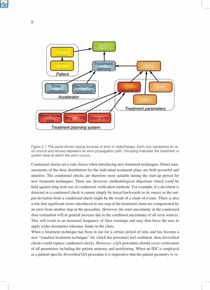
et al., 2001). For advanced radiotherapy applications with time-variable fluence patterns and steep dose gradients, the usefulness of traditional in-vivo applications can be questioned. A more advanced approach is to perform in-vivo dosimetry with an electronic portal imaging device (EPID), which means that the patient exit dose is measured and compared with a corresponding dose calculation where the patient has been accounted for. In this way the position and anatomy of the patient is integrated together with the delivered dose into the verification procedure, but also into the total uncertainty of the method. 2D and 3D in-vivo approaches based on portal dosimetry are currently explored in research institutions (McDer-mott et al., 2006, 2007; Steciw et al., 2005; van Elmpt et al., 2008; Wendling et al., 2006). Other typical condensed checks, besides in-vivo dosimetry, are verification measurements of dose distributions in 2D for a patient-specific treatment plan prior to the first treatment, e.g. experimental IMRT verification of a hybrid plan with films. Successful tests of this kind are a strong indication that the dose calculation was performed correctly, that the data transfer from the TPS to the accelerator was correct, that no changes were made in the record and ve-rify system, that the accelerator set the collimator positions correctly and that the accelerator was correctly calibrated. If any error is detected, other procedures are required to identify its origin. Condensed and diversified check procedures are in principal totally different and have speci-fic advantages and disadvantages. Figure 2.1 illustrates typical sources of error in radiothe-rapy, indicated by boxes. The arrows represent possible error propagation paths. A condensed check is typically implemented at the treatment level while a diversified QA program focuses on all different factors of influence with dedicated but independent procedures. For example, the plan transfer is verified for each patient, mechanical and dosimetric parameters of the ac-celerator are checked with various periodic quality control actions, and the dose calculation of the TPS is verified with an IDC for each patient plan. But IDC can be the method of choice to verify the performance of the TPS and check whether systematic errors have been intro-duced during commissioning or if there are uncertainties in the dose calculation algorithm of the TPS for specific treatment geometries.
8
Figure 2.1 The panel shows typical sources of error in radiotherapy. Each box represents an er-ror source and arrows represent an error propagation path. Grouping indicates the treatment or system level at which the error occurs.
Condensed checks are a safe choice when introducing new treatment techniques. Direct mea-surements of the dose distribution for the individual treatment plans are both powerful and intuitive. The condensed checks are therefore most suitable during the start-up period for new treatment techniques. There are, however, methodological objections which could be held against long term use of condensed verification methods. For example, if a deviation is detected in a condensed check it cannot simply be traced backwards to its source as the out-put deviation from a condensed check might be the result of a chain of events. There is also a risk that significant errors introduced in one step of the treatment chain are compensated by an error from another step in the procedure. However, the total uncertainty in the condensed dose estimation will in general increase due to the combined uncertainty of all error sources. This will result in an increased frequency of false warnings and may thus force the user to apply wider dosimetric tolerance limits in the clinic.When a treatment technique has been in use for a certain period of time and has become a new “standard treatment technique” for which the personnel feel confident, then diversified checks could replace condensed checks. However, a QA procedure should cover verification of all parameters including the patient anatomy and positioning. When an IDC is employed as a patient-specific diversified QA procedure it is imperative that the patient geometry is ve-
TreatmentPatient Set-up
Treatment delivery
Treatment Database
Dose calculation
Dose calibration
Mechanicalcalibration
Manual editing
Informationtransfer
Accelerator
Treatment parameters
Basic beamdata Bug in TPS User error
Treatment planning system
Patient anatomyPatient
TreatmentPatient Set-up
Treatment delivery
Treatment Database
Dose calculation
Dose calibration
Mechanicalcalibration
Manual editing
Informationtransfer
Accelerator
Treatment parameters
Basic beamdata Bug in TPS User error
Treatment planning system
Patient anatomyPatient
9The concept of independent dose calculation
rified separately on an everyday basis. Advantages of diversified checks are that the workload is not directly proportional to the number of patients and that each check can be individu-ally optimized with respect to accuracy and workload. The main disadvantage of diversified checks is that they put a large demand on the hazard analysis in order to guarantee the overall procedure. Until the workflow is under full control the condensed checks serve well as a final safety net in the QA chain.
2.2 praCtICal aspeCts oF Independent dose CalCulatIons
The goal of a routine pre-treatment verification procedure is to catch errors before the actual treatment begins. Efficient IDC can also reduce workload dramatically for advanced treat-ment techniques and it offers an alternative to experimental methods for patient-specific QA in IMRT. In order to verify multiple beams in an efficient way, one should be able to import treatment plan data (e.g. MLC settings) directly from the TPS, the oncology information system or the record and verify system. Such an automated data transfer can be realized utilizing the DICOM- RT data exchange protocol. For any calculation that is based predominately on an automated computerized approach single beam and multiple beam verification procedures do not differ significantly from a workload perspective. It is important to consider dose or monitor unit deviations in absolute as well as relative units. For IMRT deviations that are large in relative terms, but acceptable in absolute terms, predominantly in areas outside the high dose region have been reported (Baker et al., 2006; Chen et al., 2002; Linthout et al., 2004). In this region any dose calculation is largely affected by collimator transmission and penumbra modelling. It can be argued that the algorithm of the verification software needs to be at least as accurate as the TPS, in order to actually gain relevant information related to the dose calculation accuracy of the TPS. More details related to tolerance and action limits and the associated workload are discussed in chapter 3.An important current limitation with respect to IDC methods is that verification calculations are typically performed in a flat homogeneous phantom (water) for each individual beam or in a homogeneous verification phantom for composite treatment plans. This represents also the current practice for QA related to IMRT, i.e. anatomic information and inhomogeneities are in most cases not considered. As an exception the independent dose calculation approach that was presented by Chen et al (2002) for serial tomotherapy included at least the external patient contour. However, a full 3D verification calculation based on the patient CT data set is largely dependent on the availability of appropriate calculation tools in the IDC software. At present, most commercial and in-house developed solutions for IDC are not capable of recalculation on patient CT data sets. As long as patient anatomy is not included in verification calculations the accuracy of IDC is influenced by treatment site specific factors which must be considered in the analyses. For some treatment areas, such as thorax and head and neck, accurate results cannot be achieved
10
in simple calculation conditions, i.e. a semi-infinite homogeneous phantom. With radiolo-gical depth corrections for head-and-neck treatments results that are almost as good as for pelvic treatment can be achieved (Georg et al., 2007a).Traditionally the formalisms used for IDC have been designed for calculation to a single veri-fication point in the target. This can be considered as a minimum requirement. For advanced treatment techniques, such as IMRT, the dose to organs at risk is very often the main concern and of no less importance than the dose to the target. Therefore, individual dose points in the organs at risk should be verified as well (Georg et al., 2007b). A volumetric verification is generally desirable for IMRT but it might be overkill for simpler treatments. Another concern related to the verification of multiple points is the compromise between calculation accuracy and calculation speed. Furthermore, the accuracy of verification calculations in 2D or 3D is influenced by electron transport in the build-up region and in the penumbra. For IMRT leaf and collimator transmission, and tongue and groove effects need to be considered carefully. Finally, the “dimensional” aspect of verification calculations has an impact on the definition of tolerance and acceptance criteria (Mijnheer and Georg 2008). While simple dose deviati-ons suffice for point dose verification, more advanced methods that include spatial considera-tions, e.g. the gamma-index method, are required for evaluation of 2D and 3D distributions. However, accuracy demands may differ throughout the treated volume; consequently, me-thods for variable action limits must be implemented in the evaluation.The IDC software requires commissioning, including basic beam data acquisition and pos-sibly “tuning” of the algorithm. It is important to note that measurement errors in acquired beam data will propagate as systematic uncertainties in the QA procedure. As with any other dose calculation software, IDC requires QA action itself and the performance should be va-lidated against measurements to detect such systematic errors. Any use of the calculation system outside its “specifications” might lead to severe errors, incidents or accidents. To enable adequate procedures for the detection of dose calculation errors there is a need for an analysis of the error characteristics. There are several publications, reports and online databases describing incidents and accidents in radiotherapy, e.g. IAEA Safety Reports Se-ries No. 17 “Lessons learned from accidental exposures in radiotherapy” (IAEA, 2000b) and “Investigation of an accidental exposure of radiotherapy patients in Panama” (IAEA, 2001). These sources provide an insight regarding the frequent sources for errors, their cause, se-verity and follow up actions. The reported incidents put into the public domain are mostly a selection of the discrepancies which tend to reflect mistakes with severe or potentially severe consequences for the individual patient. When discussing quality assurance and taking the entire patient population into account, minor errors affecting a large fraction of the patients also become important. A fully developed QA system for dose calculations should therefore be designed to find large occasional errors as well as enable detection of small systematic errors. In summary, an IDC is a useful diversified QA procedure for advanced photon beam tech-niques. If advanced algorithms, such as the ones described in chapter 5, are utilized, IDC

11The concept of independent dose calculation
is a powerful, versatile and flexible tool that can cover almost all photon beam delivery techniques (MLC, hard wedges, soft wedges, IMRT). Moreover, dose calculations can be performed with enhanced accuracy on-axis and off-axis. A selection of the models described in chapter 5 have been implemented and evaluated as part of the “EQUAL-Dose” software (Appendix 1) and require very little commissioning. A common place for IDC as part of a QA program consisting of various diversified checks is during the first week of treatment, pre-ferable before the first treatment and when a treatment plan has been modified. The resulting data is recommended to be stored in databases for further statistical analyses.

13
3. dosIMetrIC toleranCe lIMIts and aCtIon lIMIts
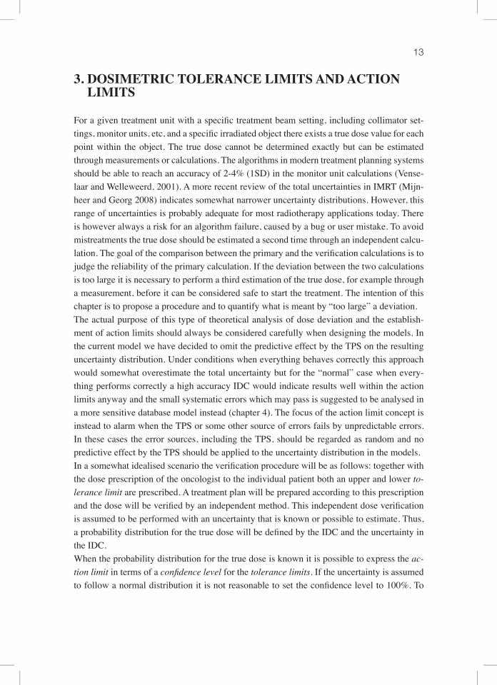
For a given treatment unit with a specific treatment beam setting, including collimator set-tings, monitor units, etc, and a specific irradiated object there exists a true dose value for each point within the object. The true dose cannot be determined exactly but can be estimated through measurements or calculations. The algorithms in modern treatment planning systems should be able to reach an accuracy of 2-4% (1SD) in the monitor unit calculations (Vense-laar and Welleweerd, 2001). A more recent review of the total uncertainties in IMRT (Mijn-heer and Georg 2008) indicates somewhat narrower uncertainty distributions. However, this range of uncertainties is probably adequate for most radiotherapy applications today. There is however always a risk for an algorithm failure, caused by a bug or user mistake. To avoid mistreatments the true dose should be estimated a second time through an independent calcu-lation. The goal of the comparison between the primary and the verification calculations is to judge the reliability of the primary calculation. If the deviation between the two calculations is too large it is necessary to perform a third estimation of the true dose, for example through a measurement, before it can be considered safe to start the treatment. The intention of this chapter is to propose a procedure and to quantify what is meant by “too large” a deviation. The actual purpose of this type of theoretical analysis of dose deviation and the establish-ment of action limits should always be considered carefully when designing the models. In the current model we have decided to omit the predictive effect by the TPS on the resulting uncertainty distribution. Under conditions when everything behaves correctly this approach would somewhat overestimate the total uncertainty but for the “normal” case when every-thing performs correctly a high accuracy IDC would indicate results well within the action limits anyway and the small systematic errors which may pass is suggested to be analysed in a more sensitive database model instead (chapter 4). The focus of the action limit concept is instead to alarm when the TPS or some other source of errors fails by unpredictable errors. In these cases the error sources, including the TPS, should be regarded as random and no predictive effect by the TPS should be applied to the uncertainty distribution in the models.In a somewhat idealised scenario the verification procedure will be as follows: together with the dose prescription of the oncologist to the individual patient both an upper and lower to-lerance limit are prescribed. A treatment plan will be prepared according to this prescription and the dose will be verified by an independent method. This independent dose verification is assumed to be performed with an uncertainty that is known or possible to estimate. Thus, a probability distribution for the true dose will be defined by the IDC and the uncertainty in the IDC. When the probability distribution for the true dose is known it is possible to express the ac-tion limit in terms of a confidence level for the tolerance limits. If the uncertainty is assumed to follow a normal distribution it is not reasonable to set the confidence level to 100%. To
14
keep the right balance between risk and workload, the procedures must include an accepted risk level for doses delivered outside the specified tolerance limits.
Figure 3.1 Illustration of parameters related to an IDC procedure. It is important to realise that an IDC is associated with an uncertainty distribution and a confidence interval Cα. The Gaussian curve represents the assumed probability density function of the true dose to the target.
The prescribed dose DP is identical to the dose specification in the TPS and is the prescribed dose to be delivered to the patient. The true dose DT is the true value of the delivered dose. The IDC dose DIDC is the dose value obtained by the independent dose calculation. The beam parameters and monitor unit settings as calculated by the treatment planning system are used as input parameters in the independent dose calculation.The true dose deviation ∆D is defined as the difference DP - DT. The normalised true dose deviation ∆ is defined as ∆D normalized to a reference dose, e.g. DP for verification points in the tumour volume. The observed dose deviation δD is defined as the difference between the prescribed dose DP and the dose obtained by the independent dose calculation system DIDC. The normalised observed dose deviation δ is the normalised difference DP – DIDC δ= –––––––––– (3.1) DIDC
The dose calculation uncertainty σ is here defined as the estimated one standard deviation of the DIDC estimation of the true dose DT.The dosimetric confidence interval Cα is the confidence interval for the 1 – α confidence level CL in an estimation of the true dose DT, where α describes the fraction of deviations outside
Risk for“injury”
Risk for“no cure”
Prescribeddose
α/2
IDC-calculation
αC
Dp TLΔ+TLΔ-
δD
DIDCDose
Pro
bab
ility
den
sity
Risk for“injury”
Risk for“no cure”
Prescribeddose
αCCCα α/2
IDC-calculation
α
Dp TLΔ+TLΔ-
δD
DIDCDose
Pro
bab
ility
den
sity
C
15Dosimetric Tolerance Limits and Action Limits
the confidence interval in a normal distributed dataset. The one-sided deviation (α/2) is de-fined for applications where only one tail of the statistical distribution is of interest. Typical values are CL=95% giving α=5% and α/2=2.5%. The dosimetric tolerance limits TL∆– and TL∆+ are defined as the lower and upper maximum true dose deviations from the prescribed dose which could be accepted based on the treat-ment objectives, treatment design and other patient-specific parameters. When the dosimetric tolerance limits are applied as offset from the prescribed dose and TL∆+ = - TL∆- the symbol TL∆ may be used for both. The use of lower and upper action limits, ALδ- and ALδ+ , is recommended to specify the li-mits at which a dose deviation from the independent dose calculation should lead to further investigations. Action limits could be based on different objectives. In a strict formalistic ap-proach a proper action limit should be determined from dosimetric tolerance limits TL∆± and the confidence interval Cα for the true dose. When the action limits are applied as offset from the prescribed dose and ALδ+ = - ALδ– the symbol ALδ– may be used for both.The parameters defined above can be applied on different dose scales depending on the cur-rent application.When presenting tolerance limits and action limits in general terms, the absolute dose scale may be impractical to use. However, when setting these parameters for an individual patient the absolute dose scale may be more relevant as the prescription dose to the tumour always is given in absolute dose. For the surrounding normal tissues and critical organs the prescribed dose is not relevant and the only parameter which is actually used is the upper tolerance limit, TL∆+. The upper action limit can then be calculated based on TL∆+ and Cα.These dose-related parameters can be given either in absolute terms, Gy, or in relative terms. In general presentations of deviations, tolerance limits and action limits the normalized re-lative dose concept is often preferred. Patient specific data as applied in the clinic may be of either type or a combination. However, special care is required when transferring parameters from relative to absolute or when transforming parameters from one relative reference sys-tem to another.
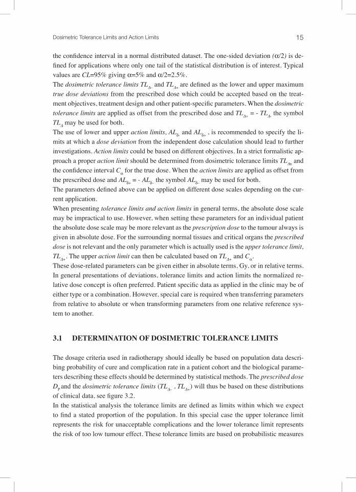
3.1 deterMInatIon oF dosIMetrIC toleranCe lIMIts
The dosage criteria used in radiotherapy should ideally be based on population data descri-bing probability of cure and complication rate in a patient cohort and the biological parame-ters describing these effects should be determined by statistical methods. The prescribed dose DP and the dosimetric tolerance limits (TL∆– , TL∆+) will thus be based on these distributions of clinical data, see figure 3.2. In the statistical analysis the tolerance limits are defined as limits within which we expect to find a stated proportion of the population. In this special case the upper tolerance limit represents the risk for unacceptable complications and the lower tolerance limit represents the risk of too low tumour effect. These tolerance limits are based on probabilistic measures
16
and should thus be treated as stochastic variables. This will in principal have an impact on the determination and interpretation of the action limits for the observed dose deviation. This is however out of the scope in this work and will not be discussed further.
Figure 3.2 Illustration of the procedure to obtain dosimetric tolerance limits from TCP and NTCP data. TL∆– is set to a minimum acceptable cure rate and TL∆+ to a maximum acceptable compli-cation rate.
The data used to determine the prescription dose and the dosimetric tolerance limits should ideally be obtained from clinical treatment outcome studies. The data could preferably be fitted to biological models as illustrated in figure 3.2. Tumour control probability (TCP) and normal tissue complication probability (NTCP) models with different endpoints are suitable for this purpose. Clinical data for these models are currently sparse but an increasing amount of clinical trials outcomes data and data based on clinical experience are being collected and analysed with respect to these biological models. There are however considerable uncer-tainties in the currently available tumour and normal tissue response data and this is why dosimetric tolerance limits in the everyday clinical practice often are set on an ad hoc basis rather than based on clinical outcome studies.General tolerance limits for dose deviations suggested in the literature are based on either rather simple biological considerations (Brahme et al., 1988) or practical experience from analyses of the accuracy of treatment planning systems (Fraass et al., 1998), (Venselaar and Welleweerd, 2001). These tolerances have in general been used in evaluation of treatment planning systems. They are also differently normalized e.g. reference dose on beam axes or
0
1
30 50 70 90
Dose / Gy
Pro
bab
ilit
y
NTCP
TCP
TL∆+TL∆-
0
1
30 50 70 90
Dose / Gy
Pro
bab
ilit
y
NTCP
TCP
TL∆+TL∆-

17Dosimetric Tolerance Limits and Action Limits
local dose. When applying these kinds of tolerance limits from the literature it is important to verify how they were determined and normalized. Typical suggested tolerance limits range from 2% at the reference point for simple beams and up to 50% outside the beam edge in more complex cases if normalized to the local dose. If the deviation is normalized to a point in the high dose region such as the prescribed dose the suggested range of tolerance limits would vary between approximately 2 and 5 %.
3.2 the aCtIon lIMIt ConCept
According to the EURATOM directive 97/43 (EURATOM, 1997) there must be an inde-pendent dose verification procedure involved in all clinical radiation therapy routines. This procedure can be performed by different methods and typically results in an observed dose deviation. The choice of action limit is in many clinics based on ad hoc values dictated by practical limitations rather than systematic analyses of statistical uncertainties and error propagation. With estimated uncertainties provided by the QA tools and the possibility to analyse QA data in databases the statistical behaviour of the different components should be better understood.

18
Figure 3.3 Illustration of a method of calculating action limits (indicated by the vertical bars) from given dosimetric tolerance limits, TL∆ = 8% and a= 5%. In panel a) the uncertainty of the IDC is set to σ = 1% , in panel b) σ= 2% and in panel c) no significant uncertainty in the IDC was as-sumed. The curves in the panels show the assumed probability distribution of the true dose. For the central curve the IDC indicates no dose deviation from the prescribed dose, while the curves to the left and the right show the assumed distribution of the true dose when the IDC doses are such that α/2 of the normal distributed true dose is outside the dosimetric tolerance limit. The centre of the latter distributions thus represents the action limit.
The method used to set proper action limits must include the statistical uncertainty of the IDC which gives the confidence interval (Cα) for the true dose. The action limits should be calculated as CαALδ= TL∆ +––– (3.2) 2
where Cαdescribe the uncertainty of the IDC. Figure 3.3 illustrates the relation between the IDC uncertainty and the proper action limits. The dosimetric tolerance limits are in all cases set to TL∆± = 8% and the confidence level is set to 95% (α/2=2.5%). Figure 3.3a) illustrates a case where the standard deviation of the IDC is 1% (σ = 1%). The 95% confidence interval for the true dose around the IDC calculation will in this case be ± 2% (Cα=±2%). According to equation 3.2 the resulting action limits will in this case be ±6% (ALδ± =±6%) as illustrated in the figure. Figure 3.3 b illustrates a more realistic case with an IDC uncertainty σ = 2% resulting in action limits ALδ± =±4%. A rather unrealistic case with no assumed uncertainty
σ=1%
σ=2%
σ=0%
Pro
bab
ility
den
sity
+∆TL-∆TL
α/2
α/2
α/2
-∆AL +∆AL
+∆AL
+∆AL-∆AL
-∆AL
a)
b)
c)
σ=1%
σ=2%
σ=0%
Pro
bab
ility
den
sity
+∆TL-∆TL
α/2
α/2
α/2
-∆AL +∆AL
+∆AL
+∆AL-∆AL
-∆AL
σ=1%
σ=2%
σ=0%
Pro
bab
ility
den
sity
+∆TL-∆TL
α/2
α/2
α/2
-∆AL +∆AL
+∆AL
+∆AL-∆AL
-∆AL
a)
b)
c)
19Dosimetric Tolerance Limits and Action Limits
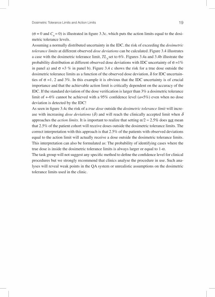
(σ = 0 and Cα=0) is illustrated in figure 3.3c, which puts the action limits equal to the dosi-metric tolerance levels. Assuming a normally distributed uncertainty in the IDC, the risk of exceeding the dosimetric tolerance limits at different observed dose deviations can be calculated. Figure 3.4 illustrates a case with the dosimetric tolerance limit, TL∆ set to 6%. Figures 3.4a and 3.4b illustrate the probability distribution at different observed dose deviations with IDC uncertainty of σ =1% in panel a) and σ =3 % in panel b). Figure 3.4 c shows the risk for a true dose outside the dosimetric tolerance limits as a function of the observed dose deviation, δ for IDC uncertain-ties of σ =1, 2 and 3%. In this example it is obvious that the IDC uncertainty is of crucial importance and that the achievable action limit is critically dependent on the accuracy of the IDC. If the standard deviation of the dose verification is larger than 3% a dosimetric tolerance limit of +-6% cannot be achieved with a 95% confidence level (a=5%) even when no dose deviation is detected by the IDC!As seen in figure 3.4c the risk of a true dose outside the dosimetric tolerance limit will incre-ase with increasing dose deviations (δ ) and will reach the clinically accepted limit when δapproaches the action limits. It is important to realize that setting α/2=2.5% does not mean that 2.5% of the patient cohort will receive doses outside the dosimetric tolerance limits. The correct interpretation with this approach is that 2.5% of the patients with observed deviations equal to the action limit will actually receive a dose outside the dosimetric tolerance limits. This interpretation can also be formulated as: The probability of identifying cases where the true dose is inside the dosimetric tolerance limits is always larger or equal to 1-α. The task group will not suggest any specific method to define the confidence level for clinical procedures but we strongly recommend that clinics analyse the procedure in use. Such ana-lyses will reveal weak points in the QA system or unrealistic assumptions on the dosimetric tolerance limits used in the clinic.
20
Figure 3.4 Illustration of the probability of patients exceeding the assumed tolerance limits of 6% as a function of observed dose deviation, δ. Panels a) and b) illustrate the IDC uncertainty when the observed dose deviation is 0 and +-6%. The IDC uncertainty is set to σ =1% in panel a and in panel b to σ =3%. Panel c) illustrates the probability of exceeding the tolerance limits as a function of the observed dose deviation, δ for IDC uncertainties σ =1, 2 and 3%.
The prescribed dose to the tumour and the tolerance limits are in general applied in the high dose region but in a more detailed analysis of the treatment plan there is a need for methods that can be applied also in the low dose regions as well as in gradient regions. For the sur-rounding normal tissue separate dose criteria may be used, often represented by only the upper tolerance limit applied to some equivalent uniform dose quantity dependent on the characteristics of the tissue. Historically the low dose regions have been regarded as less significant and have in general not been simulated to the same level of accuracy in the treatment modelling. This may be clinically relevant for the target dose but in modelling of side effects correct dose estimations in the low dose regions may also be crucial. In the current report we suggest that action limits related to target tissue should be applied to the absolute dose deviation or relative dose nor-malized to the prescribed dose. By this method the importance of deviations in the low dose
σ = 1%P
rob
. dev
iati
on
> T
L
δ/%
+∆TL-∆TL
Pro
bab
ility
den
sity
σ = 3%
σ = 3%σ = 2%σ = 1%
α=5%
a)
b)
c)
σ = 1%P
rob
. dev
iati
on
> T
L
δ/%
+∆TL-∆TL
Pro
bab
ility
den
sity
σ = 3%
σ = 3%σ = 2%σ = 1%
α=5%
a)
b)
c)
21Dosimetric Tolerance Limits and Action Limits
regions will automatically decrease. It is further suggested that the action limits related to normal tissues should be specified as absolute dose limits. However, care must be taken to ap-ply correct dose deviation uncertainties for the IDC in the application of these action limits.For IMRT-methods the combined uncertainty will be more complex to analyse. The total uncertainty of the IDC will thus be a result of the combined uncertainties of the individual dosimetry points in the contributing beams. In IMRT and other more complex applications these beam combinations will include the increased uncertainties at off-axis positions, the uncertainty in high dose gradient regions and even the dose uncertainty outside the beam. This combined uncertainty effect may be described by a pure statistical approach where ef-fects in gradient regions due to a number of clinical error sources may be included (Jin et al., 2005) or by more detailed analysis of the underlying physics (Olofsson et al., 2006a; Olofs-son et al., 2006b). The latter method will inevitably give more details regarding the actual IDC calculation. However, in the full prediction of the overall uncertainty other error sources such as set-up uncertainties will also affect the gradient regions and should thus be included. For this purpose a combination of methods may produce more realistic over-all uncertainty estimations when performing dose verification in dose gradient regions.
3.3 applICatIon oF the aCtIon lIMIt ConCept In the ClInIC
When utilizing the action limit concept in clinical practice as illustrated in figures 3.2 and 3.3 the relationship between the action limit, ALδ, the chosen tolerance limits, TL∆, the correspon-ding α-value, and the estimated one standard deviation uncertainty, σ, of the independently calculated dose by the IDC not trivial. For illustration the relations between these parameters have been plotted in figure 3.4 for different assumed σ-values and observed dose deviations. When the parameters TL∆ and α have been selected and the σ of the independent dose verifi-cation procedure is known the action limits, ALδ, can be determined from this figure.

22
Figure 3.5 The vertical axis shows the action limit normalized to the estimated standard deviation σtotal for the independent dose calculation, IDC. The horizontal axis represents α. The six curves represent varying relations between the dosimetric tolerance limit TL∆ and σtotal.
The use of figure 3.5 may be illustrated by some numerical examples. If TL∆ = 3.6%, a= 5%, the standard deviation σtot for IDC calculation is estimated to 1.2% (i.e. TL∆ /σ =3), then ALδ / σ≈ 1.4 which gives the proper action limit ALδ ≈ 1.7% (this example is indicated as a dot in figure 3.5). If σ would have been twice as large (i.e. 2.4%) the ratio TL∆ /σtot would be 1.5, thus yielding an action limit of zero (provided that the chosen levels for TL∆ and α remain unchanged). Consequently, the estimated risk for the true dose being outside prescribed to-lerance interval TL∆ will always be larger than the established probability, a=5%, even when no deviation is found by the independent dose calculation, e.g. δ = 0. The conclusion of this exercise is that the accuracy of the independent dose calculation is of crucial importance when applying a strict action limit concept. When the data for TL∆, α,and σtot are known the action limits, AL∆ , can be directly calculated by equation 3.2 or interpolated from figure 3.5. Selecting the commonly used 95% confi-dence level, α/2 = 0.025, implies a confidence interval of 1.96 σtot. For evaluation of treat-ment planning systems Venselaar et al (Venselaar and Welleweerd, 2001) suggested to use a confidence interval of 1.5 σtot , which corresponds to a one-sided α, α/2 = 0.065. This more relaxed choice of confidence interval may be practical for many clinical applications. For a fixed value of α/2 = 6.5% the action limits can be directly determined from equation 3.4.
1.5·σtotAL∆= TL∆ – ––––––– (3.3) 2
23Dosimetric Tolerance Limits and Action Limits
If the IDC calculation utilizes a simple phantom geometry that is very different from the anatomy of the patent the total uncertainty of the IDC will increase. However, there may be a significant systematic component in these deviations that should be recognized as such. Georg et al (Georg et al., 2007a) illustrate deviations when radiological depths were applied and when they were not. Application of radiological depth corrections significantly redu-ced the observed dose deviations. The resulting IDC uncertainty must however include the uncertainty in the radiological depth correction but the resulting total uncertainty is now ap-proximately of a random nature and if known could be used to determine proper action limits.In general, complicated treatments should not have larger action limits than conventional treatments. A strict application of the action limit concept is a reasonable way of handling de-viations from a patient perspective. However from a more practical clinical perspective this may in some special cases not be realistic. The final decision to clinically apply a treatment plan, in spite of the fact that an action limit has been exceeded, must be thoroughly discussed and documented for every treatment. Under special circumstances, when the source of a de-viation cannot be found with available resources, the overall patient need must be weighed against the risk of a true dose deviation larger than the tolerance limits. In these cases the action limit can no longer be considered as restrictive. Since the clinical relevance of a pa-rameter can differ considerably from one treatment to another, it is impossible to implement action limits as a mandatory requirement. When these treatments are correctly documented the size and frequency of dose deviations larger than the action limit should be stored in a database and used as a quality parameter in the clinic to be considered in the planning of QA resources at the clinic.The concept of uncertainty applied in this booklet is based on the ISO “Guide to the expres-sion of uncertainty in measurement” GUM 1995, revised version (ISO/GUM, 2008) . For further reading and application of GUM, see e.g. www.bipm.org or www.nist.gov.

25
4. statIstICal analysIs
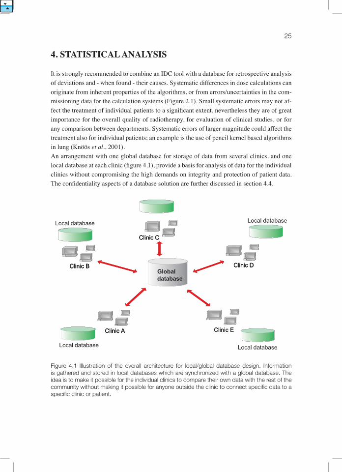
It is strongly recommended to combine an IDC tool with a database for retrospective analysis of deviations and - when found - their causes. Systematic differences in dose calculations can originate from inherent properties of the algorithms, or from errors/uncertainties in the com-missioning data for the calculation systems (Figure 2.1). Small systematic errors may not af-fect the treatment of individual patients to a significant extent, nevertheless they are of great importance for the overall quality of radiotherapy, for evaluation of clinical studies, or for any comparison between departments. Systematic errors of larger magnitude could affect the treatment also for individual patients; an example is the use of pencil kernel based algorithms in lung (Knöös et al., 2001). An arrangement with one global database for storage of data from several clinics, and one local database at each clinic (figure 4.1), provide a basis for analysis of data for the individual clinics without compromising the high demands on integrity and protection of patient data. The confidentiality aspects of a database solution are further discussed in section 4.4.
Figure 4.1 Illustration of the overall architecture for local/global database design. Information is gathered and stored in local databases which are synchronized with a global database. The idea is to make it possible for the individual clinics to compare their own data with the rest of the community without making it possible for anyone outside the clinic to connect specific data to a specific clinic or patient.
Clinic A
Clinic B
Clinic C
Clinic D
Clinic E
Global database
Local database
Clinic AClinic A
Clinic BClinic B
Clinic CClinic C
Clinic DClinic D
Clinic E
Local database
Local database
Local database
26
The basic concept behind the database solution proposed here is that all relevant information related to the commissioning of the system and generated during the verification process should be transferred to both a local statistical database and a global database. The local database will only contain data generated locally in a department while the global database contains data from users of all applications interfacing with the global database server. The users can thus compare results obtained locally with the results of the community through such a solution.The clinical value of a global database is strongly related to the amount of stored information and the quality of the information (see section 4.4). A global database should be equipped with a standardized interface towards the outside to enable different vendors and applications to take advantage of such a solution. This is a natural step in the globalization and standardi-zation of healthcare data storage without compromising the integrity of patients or hospitals. During the current ESTRO task project a global database for IDC data has been made avai-lable, see appendix 1 for further details.
4.1 database applICatIon For CoMMIssIonIng data
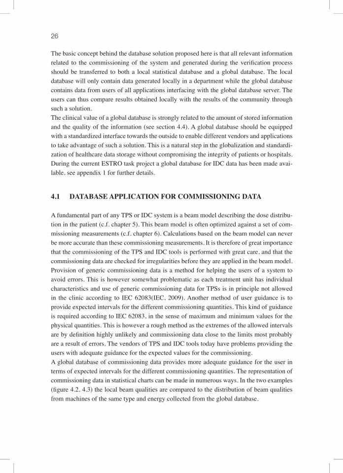
A fundamental part of any TPS or IDC system is a beam model describing the dose distribu-tion in the patient (c.f. chapter 5). This beam model is often optimized against a set of com-missioning measurements (c.f. chapter 6). Calculations based on the beam model can never be more accurate than these commissioning measurements. It is therefore of great importance that the commissioning of the TPS and IDC tools is performed with great care, and that the commissioning data are checked for irregularities before they are applied in the beam model. Provision of generic commissioning data is a method for helping the users of a system to avoid errors. This is however somewhat problematic as each treatment unit has individual characteristics and use of generic commissioning data for TPSs is in principle not allowed in the clinic according to IEC 62083(IEC, 2009). Another method of user guidance is to provide expected intervals for the different commissioning quantities. This kind of guidance is required according to IEC 62083, in the sense of maximum and minimum values for the physical quantities. This is however a rough method as the extremes of the allowed intervals are by definition highly unlikely and commissioning data close to the limits most probably are a result of errors. The vendors of TPS and IDC tools today have problems providing the users with adequate guidance for the expected values for the commissioning.A global database of commissioning data provides more adequate guidance for the user in terms of expected intervals for the different commissioning quantities. The representation of commissioning data in statistical charts can be made in numerous ways. In the two examples (figure 4.2, 4.3) the local beam qualities are compared to the distribution of beam qualities from machines of the same type and energy collected from the global database.
27Statistical analysis
Figure 4.2 Profiles measured for Siemens 6MV beams are collected from a global database and compared to a locally measured profile. The 10% and 90% percentiles are provided to indicate a normal interval for the measured profiles.
Figure 4.3 Histogram showing the distribution of TPR20/10 for Elekta 6MV beams. The local observation is indicated with the thin bar.
-20 -10 0 10 20
96
98
100
102
104
Position (cm)
Rel
ativ
e do
se (%
)
Local measurementGlobal MedianGlobal 10 resp. 90% percentile
0.66 0.67 0.68 0.69 0.7
Fre
qu
ency
TPR 20/10
0.66 0.67 0.68 0.69 0.70.66 0.67 0.68 0.69 0.7
Fre
qu
ency
TPR 20/10
28
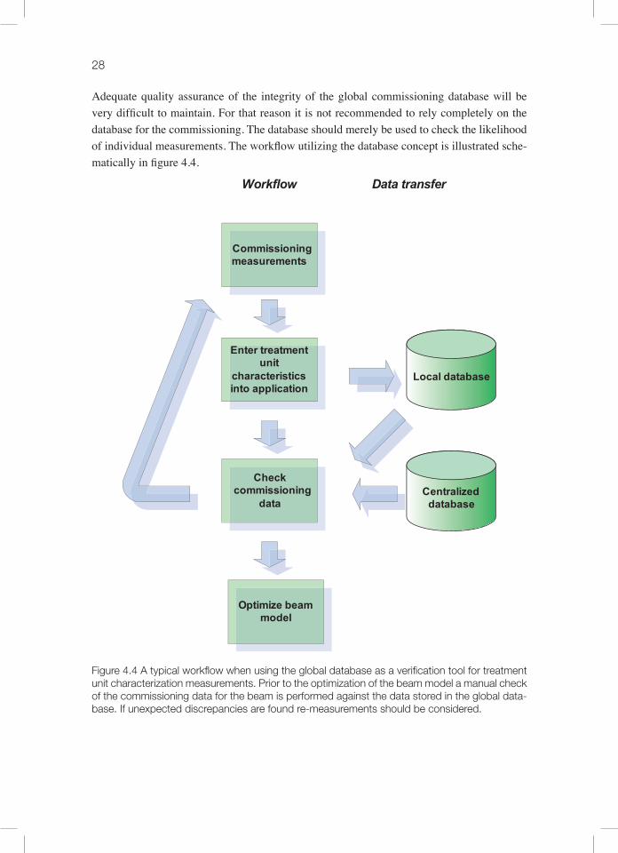
Adequate quality assurance of the integrity of the global commissioning database will be very difficult to maintain. For that reason it is not recommended to rely completely on the database for the commissioning. The database should merely be used to check the likelihood of individual measurements. The workflow utilizing the database concept is illustrated sche-matically in figure 4.4.
Figure 4.4 A typical workflow when using the global database as a verification tool for treatment unit characterization measurements. Prior to the optimization of the beam model a manual check of the commissioning data for the beam is performed against the data stored in the global data-base. If unexpected discrepancies are found re-measurements should be considered.
Commissioning measurements
Enter treatment unit
characteristics into application
Local database
Centralized database
Check commissioning
data
Optimize beam model
Data transferWorkflow
29Statistical analysis
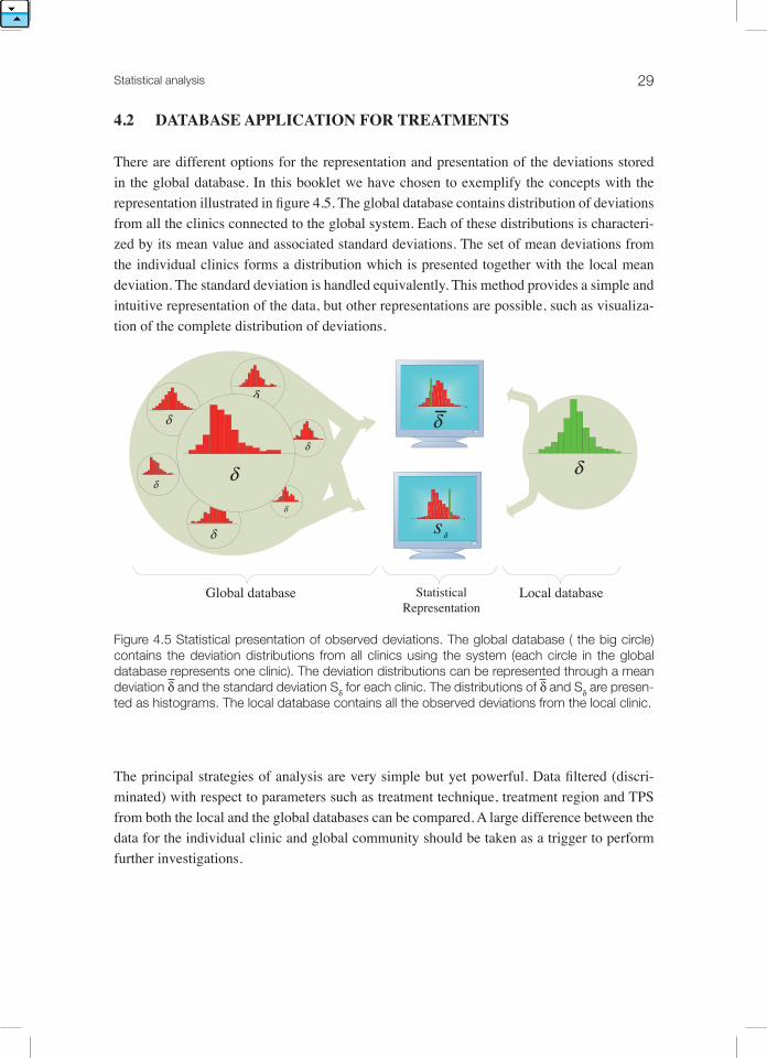
4.2 Databaseapplicationfortreatments
There are different options for the representation and presentation of the deviations stored in the global database. In this booklet we have chosen to exemplify the concepts with the representation illustrated in figure 4.5. The global database contains distribution of deviations from all the clinics connected to the global system. Each of these distributions is characteri-zed by its mean value and associated standard deviations. The set of mean deviations from the individual clinics forms a distribution which is presented together with the local mean deviation. The standard deviation is handled equivalently. This method provides a simple and intuitive representation of the data, but other representations are possible, such as visualiza-tion of the complete distribution of deviations.
Figure 4.5 Statistical presentation of observed deviations. The global database ( the big circle) contains the deviation distributions from all clinics using the system (each circle in the global database represents one clinic). The deviation distributions can be represented through a mean deviation δ and the standard deviation Sδ for each clinic. The distributions of δ and Sδ are presen-ted as histograms. The local database contains all the observed deviations from the local clinic.
The principal strategies of analysis are very simple but yet powerful. Data filtered (discri-minated) with respect to parameters such as treatment technique, treatment region and TPS from both the local and the global databases can be compared. A large difference between the data for the individual clinic and global community should be taken as a trigger to perform further investigations.
ss
δ
δ
δ
δ
δ
δ
δ
δ
δ
Global database StatisticalRepresentation
Local database
δ
30
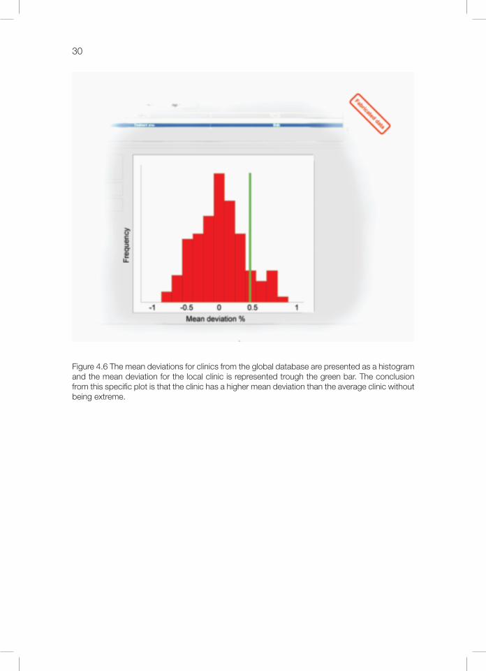
Figure 4.6 The mean deviations for clinics from the global database are presented as a histogram and the mean deviation for the local clinic is represented trough the green bar. The conclusion from this specific plot is that the clinic has a higher mean deviation than the average clinic without being extreme.

31Statistical analysis
Figure 4.7 The standard deviation for the observed discrepancies for all individual clinics can be collected from the global database and presented in the histogram. The standard deviation for the deviations at the individual clinic is given by the green bar. The conclusion in this case is that the intra-patient variation at the clinic is on the lower side of the global distribution.
The data selection/discrimination is an essential part of the analysis. The overall distribution includes samples from sub-distributions as illustrated in figure 4.8. A discrepancy between the results at an individual clinic and the rest of the community does not automatically mean that something is wrong at the individual clinic. It could be caused by differences in verifica-tion routines or differences in treatment technique and equipment. For instance, a clinic with a focus on stereotactic treatments of metastasis in the brain should expect to get different de-viation patterns than clinics that mainly perform whole brain treatments. The analysis of the deviation pattern does therefore need to be performed by qualified personnel able to interpret the results and refine the comparison until relevant conclusions can be made. An exemple of such a procedure is provided in figure 4.9.
Fabricated data

32
Figure 4.8 The overall distribution of deviations in the top row of the figure represent the pooled data of the sub-distributions presented at the bottom. The information that is visible in the sub-distributions in the bottom is concealed in the overall distribution at the top. It is important to use evaluation filters and visualize sub-sets of the total database information in order to adequately use the database concept.
Fabricated data

33Statistical analysis
Figure 4.9 This example of a possible analysis pathway starts with a comparison on the treat-ment level for treatments towards the pelvis region (A). A tendency of lower doses than average is noticed. In order to identify the reason for this tendency a comparison for individual beams towards the pelvis region is performed (B,C). In this comparison an additional classification with respect to the gantry angle is added. (B) shows the deviation for beams entering from the anterior or posterior of the patient. The tendency of lower doses than average cannot be seen here. (C) shows the deviations for the lateral beams. Based on this investigation a possible reason for the initially observed low doses for the pelvis treatments could be that the clinic does not adjust for the radiological depth in the verification calculation. In the pelvic region this could typically cause an error of a few percent in the lateral beams.
Fabricated data
34
Information regarding the local “stability”, for instance investigations of the effect of TPS upgrades and changed routines can be performed using a local database solely. The informa-tion in a local database could be seen as a time series of deviations, and should be visualized and analyzed as such. Time series analysis has been used in process industries since the early 30s for production surveillance. These methods are often referred to as statistic process con-trol or statistic quality control.
4.3 QualIty oF the database
The purpose of a database solution for IDC is to enable detection of systematic dose calcula-tion errors in individual departments. As it is assumed that systematic errors exist, they will also be represented in the database of stored deviations between calculations performed with the TPS and the IDC tool. The basic assumption is that the majority (mean) of the radiothe-rapy community follows the current state-of-the-art, and that the comparison between the individual department and the global database therefore is a comparison versus the state-of-the-art. The usefulness of a database solution for the detection of systematic errors in dose calcula-tions is highly dependent on the quality of the submitted data. There are at least three iden-tified cases of corrupt or irrelevant data in the database for which the application needs to be protected: (1) users getting experience with the application with non-clinical data but the data are accidentally pushed to the database, (2) outdated and therefore irrelevant data and (3) selected data including an ad hoc bias. A full control and maintenance of the database would be very costly and is unnecessary if the system is prepared for the cases mentioned above. For example, the risk of non-clinical data being pushed to the local and global database could be reduced by setting up both a clinical and non-clinical mode of the software, and to force the user to sign the data prior to the database submission. Alternative or combined methods can reduce the risk of outdated data being used inadventently. One possibility is to use time-discrimination where only data collected within a specified time interval is presen-ted. Another option is to include only data for treatment units that are currently in use at the departments. This could be achieved through regular updating and synchronization of the global database against the local databases and the configurations at the individual clinics. The most difficult quality aspect to control is the risk for selected (or biased) data coming from the different users, i.e. departments excluding specific patient groups or treatment tech-niques for particular reasons. No general solution is suggested to avoid this. It is basically a matter of policy at the clinics and a challenge for the developer of the systems that use data-base solutions to make the evaluation tools more selective.

35Statistical analysis
4.4 normalizationofDoseDeviations
The quality of the collection of deviations between calculations performed with the TPS and the IDC in a common global database is highly dependent on the properties of the IDC tool. In order to describe the actual information contained in such a database an in-depth analysis of the factors behind the deviations is required. In the following the patient anatomy is taken into account as a starting point. The discussion is then transferred into a more traditional case where the patient anatomy is not considered for independent dose calculations. The dose at a point calculated by the TPS can be written as a product of factors taking dif-ferent effects into account
B.M. AlgoDTPS = F (A)F (A;P) (4.1) TPS TPS
where DTPS is the dose calculated by the treatment planning system, B.M.F TPS (A) is a factor describing the specific Beam Model used including the beam commissioning applied with the treatment settings A, including collimator settings, gantry, collimator and table angles, wedges etc. AlgoF TPS (A;P) describes the algorithms in use which depends both on the treatment settings A and the representation of the patient stored in P. The dose calculated by the IDC tool (DIDC ) is expressed in the same format as used in equa-tion 4.1 according to
B.M. AlgoDICT = F (A)·F (A;P) (4.2) IDC IDC
The relative deviation between the TPS and the IDC is defined according to
DTPS – DIDC DTPSδ = ––––––––––––– = –––––– – 1 (4.3) DIDC DIDC
which can be rewritten through the factors as
B.M.F TPS (A)· AlgoF TPS (A;P)δ = ––––––––––––––––––––– – 1 (4.4) B.M.F IDC (A)· AlgoF IDC (A;P)
The first term of equation (4.4) can be considered as normalization of the TPS dose calcula-tion, using the IDC calculation and corresponds to removal of the individual characteristics of the TPS dose calculation in terms of the treatment design (A) and patient (P). This enables comparison of dose calculation results between individual patients, clinics and treatment planning systems. After such normalization, the results of equation 4.4 reflect the difference in the way the IDC and the TPS use the treatment settings and patient information to calculate the absorbed dose. If the IDC and the TPS are not completely independent the factors may cancel out, leading to a risk for undetectable errors. One example could be use of common commissioning data, which in principal leads to a cancellation of B.M.F TPS (A) and B.M.F IDC (A),
36
and thus disable detection of errors in the beam commissioning. This illustrates the impor-tance of complete independence of the IDC from the TPC.The value of the scored deviation is highly dependent on the accuracy of the IDC. A poor normalization makes any comparison between different treatments difficult. If the IDC has known limitations in specific situations, these can be dealt with using selective data compari-sons (data discrimination). An example represented in equation 4.5 is if the IDC does not take the patient geometry into consideration and instead employs calculations in a water phantom:
B.M.F TPS (A)· AlgoF TPS (A;P)δ= ––––––––––––––––––––– – 1 (4.5) B.M.F IDC (A)· AlgoF IDC (A;W)
where W indicates water. In these situations it is obvious that the deviation will be highly de-pendent on the treatment area of the patient. Treatments in the thorax region and the pelvis re-gion should not be compared. Treatments in the same treatment region however can in many cases be assumed to give similar deviations. This is one situation when a tool for data dis-crimination is of importance, e.g to enable comparisons that include only pelvis treatments. Another reason for including data discrimination is the usefulness as a tool for investigations of observed discrepancies as has been discussed in previous chapters.
4.5 ConFIdentIalIty and IntegrIty oF the database
Confidentiality is an important issue in terms of the possibility to identify individual patients, clinics, staff members and equipment. Regulations and traditions differ among countries and the over-all purpose of using an independent dose verification tool may also differ conside-rably.Patient confidentiality within the European Union is regulated in EU Directive 95/46/EC. Storage of patient data in a global database in the context of dose calculation QA is in princi-pal prohibited by the 95/46/EC directive through Article 7, unless legislation in the individual country forces the storage. The only obvious reason for storage of personal information is the scenario of third party supervision of clinics on an individual patient basis. The analysis scenarios do not depend on access to personal data. The general design of both the local and the global database can provide complete patient confidentiality, i.e. no personal data need to be stored (or sent over the internet).The identity of the treatment planning system is important information in the global database as it makes it possible for the individual clinic to compare selectively with users of their own treatment planning system. This is a natural first step in the investigation around suspect de-viations. The suggestion is that the treatment planning system as well as the software version used for primary calculation of a treatment plan should be mandatory information in both the local and the global database.
37Statistical analysis
Identification of individual clinics within a global statistical database is another type of issue that needs to be handled in an adequate manner. One would wish to keep the identities of in-dividual clinics within the database, as nobody within this application should have anything to hide. However, such an open policy may prove to be counterproductive from a QA point of view, while clinics may hesitate to use a tool where individual clinics could be identified. The recommendation is therefore to follow an intermediate path which allows the individual clinic to configure the system to reveal or hide the clinic’s name in the global database. Even if the clinic chooses anonymity it is possible to compare their own data from the local data-base with the global database. Related to the possibility to identify individual clinics is the possibility to identify individual countries or regions. As there are areas where the number of clinics is small, country or re-gion identification would in principle be equivalent to clinic identification. It is therefore also suggested that geographical information be treated as optional data in the global database. The type of treatment unit, vendor and version is suggested to be mandatory information in both the global and local statistical database for the same reason as for the treatment planning system. In general, the global database should be designed to support all collaborating clinics with reference data which are specific with respect to treatment method and equipment. All data related to individuals should be optional and protected by coding procedures. Any access to such data should be allowed only by special authorisation and would further require access to the de-coding keys.

39
5. beaM ModellIng and dose CalCulatIons
Dose calculations can be performed through various methods utilizing fairly different appro-aches. A tool for independent dose calculations, or any other kind of dose calculation device, is a compromise between the benefits and drawbacks associated with different calculation methods in relation to the demands on accuracy, speed, ease of use. The complexity of mo-dern external beam therapy techniques paired with clinical demands on efficiency require dose calculation methods that offer a high degree of generality, but still are robust and simple to use. This implies that the employed IDC calculation methods must develop into more explicit models of the physical processes that significantly influence the delivered dose. As a result the major workload for clinical implementation of an IDC tool is shifted from beam commissioning, performed by individual users, to an earlier stage of research and software development.Traditionally the most common way of calculating the dose is through a series of multiplica-tive correction factors that describe one-by-one the change in dose associated with a change of an individual treatment parameter, such as field size and depth, starting from the dose under reference conditions. This approach is commonly referred to as factor-based calcula-tion and has been the subject of detailed descriptions (Venselaar et al., 1999; Dutreix et al., 1997). The individual factors are normally structured in tables derived from measurements or described through parameterizations. Some factors can be calculated through simple model-ling, for example the inverse square law accounting for varying treatment distances. From an implementation point of view a factor-based method may be an attractive approach due to its computational simplicity, once all the required data are available. The obvious problem as-sociated with this approach is the required amount of commissioned beam data as this type of method can not calculate doses when the beam setup is not covered by the commissioned set of data. For treatment techniques that can make use of many degrees of freedom, such as the shape of an irregular field, it becomes practically impossible to tabulate or parameterize all factors needed to cover all possible cases. Hence, the factor-based approach is best suited for point dose calculations along the central beam axis in beams of simple (rectangular) shapes.The most general dose calculation method currently available is the Monte Carlo simulation, which explicitly simulates the particle transport and energy deposition through probability distributions, combining detailed geometric descriptions and fundamental radiation inter-action cross-section data. The drawbacks are related to the advanced implementation and the need for non-trivial beam commissioning as there is a requirement for fundamental pro-perties such as energy spectra and details of the treatment head design. The extensive and time-consuming calculations also limit the use of Monte Carlo methods in clinical routine, although the access to more powerful computers is causing this aspect to gradually lose re-levance.An effective method for model-based dose calculations is offered by combining multi-source modelling of the energy fluence exiting the treatment head with use of energy deposition

40
kernels describing the energy deposition in the patient through convolution/superposition with the energy fluence incident on the irradiated object. This approach utilizes the natural divider between the radiation sources inside the treatment head, consisting of air and high-density materials, and the patient or the phantom, consisting of water-like media (cf. figure 5.1). Consequently, the dose calculations can be separated into two factors, both determined through modelling:
D (x,d;A) Ψ(x;A) D(x,d;A)–––––––– = ––––––– . –––––––, (5.1) M(A) M(A) Ψ(x;A)
where D is the dose, x is an arbitrary calculation point, d is the treatment depth, A represents the treatment head setting, M is the monitor signal, and Ψ is the energy fluence. This type of model also has the advantage that it can be sufficiently characterized by a limited amount of commissioned beam data. In the following sections a more detailed description of the com-ponents involved in this dose calculation approach is given.
Figure 5.1. Schematic illustration of the separation (red dotted line) in equation (5.1) between energy fluence modelling, associated with the treatment head, and the subsequent formation of dose inside the irradiated patient/phantom.
d
Patient/ phantom
x
A
/Μ
D/Ψ
M
Treatment head
/ΜΜ
d
Patient/ phantom
x
A
Ψ /Μ
D/Ψ
M
Treatment head

Beam modelling and dose calculations 41
5.1 energy FluenCe ModellIng
In many cases the radiation source of a linear accelerator is regarded as a single point source located at the nominal focal point, normally 100 cm “upstream” from the accelerator’s iso-center. However, in reality the focal source contributes 90-97% of the energy fluence rea-ching the isocenter point, depending on the design and actual settings of the treatment head. In order to accurately model the energy fluence exiting the treatment machine the remaining significant sources must be identified and properly accounted for. Figure 5.2 shows an over-view of the principal treatment head components that form a clinical megavoltage photon beam.Following the elements of treatment head design a general expression for the resulting pho-ton energy fluence per monitor signal can be formulated as (Ahnesjö et al., 1992a; Olofsson et al., 2006b)
Ψ (x;A) Ψd(x;A) + Ψe(x;A) + Ψpw (x;A) + Ψc(x;A)–––––– = ––––––––––––––––––––––––––––––––––, (5.2) M(A) Md + Me + Mpw + Mc (A)
where the indices d, e, pw, and c in equation (5.2) denote direct (focal), extra-focal, physical wedge, and collimator contributions, respectively. These four sources also generate the dose monitor signal M, but it is only the component associated with the collimators downstream from the monitor chamber (Mc) that varies with the treatment head setting A. In sections 5.1.1 to 5.1.7 the different components of equation (5.2) will be discussed in some detail. It should, however, be noted that equation (5.2) does not include the charged particle contamination of high-energy photon beams that will be further discussed in section 5.2.2.
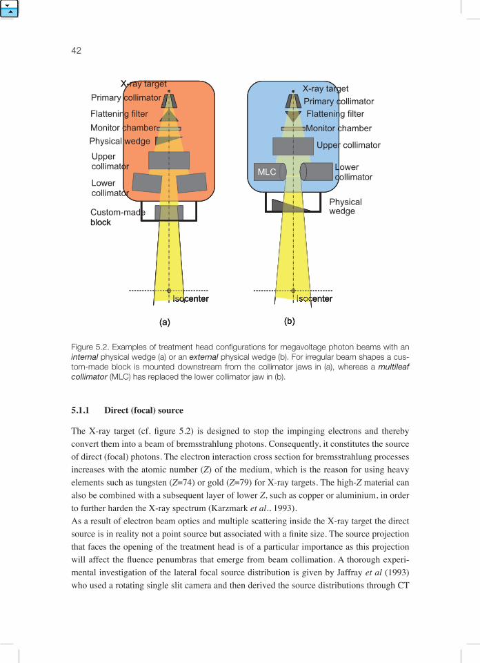
42
Figure 5.2. Examples of treatment head configurations for megavoltage photon beams with an internal physical wedge (a) or an external physical wedge (b). For irregular beam shapes a cus-tom-made block is mounted downstream from the collimator jaws in (a), whereas a multileaf collimator (MLC) has replaced the lower collimator jaw in (b).
5.1.1 direct (focal) source
The X-ray target (cf. figure 5.2) is designed to stop the impinging electrons and thereby convert them into a beam of bremsstrahlung photons. Consequently, it constitutes the source of direct (focal) photons. The electron interaction cross section for bremsstrahlung processes increases with the atomic number (Z) of the medium, which is the reason for using heavy elements such as tungsten (Z=74) or gold (Z=79) for X-ray targets. The high-Z material can also be combined with a subsequent layer of lower Z, such as copper or aluminium, in order to further harden the X-ray spectrum (Karzmark et al., 1993).As a result of electron beam optics and multiple scattering inside the X-ray target the direct source is in reality not a point source but associated with a finite size. The source projection that faces the opening of the treatment head is of a particular importance as this projection will affect the fluence penumbras that emerge from beam collimation. A thorough experi-mental investigation of the lateral focal source distribution is given by Jaffray et al (1993) who used a rotating single slit camera and then derived the source distributions through CT
X-ray target
Isocenter
Custom-made block
(a)
X-
Physical wedge
MLC
enter
(b)
Isocenter
(a)
IIssooIsocenter
(a)
X-
MLC
enter
(b)
ray target
Flattening filterMonitor chamber
Upper collimator
Primary collimatorX-
MLC
Isocenter
(b)
Lower collimator
X-ray target
block
Flattening filterMonitor chamber
Upper collimator
Lower collimator
Primary collimator
Physical wedge
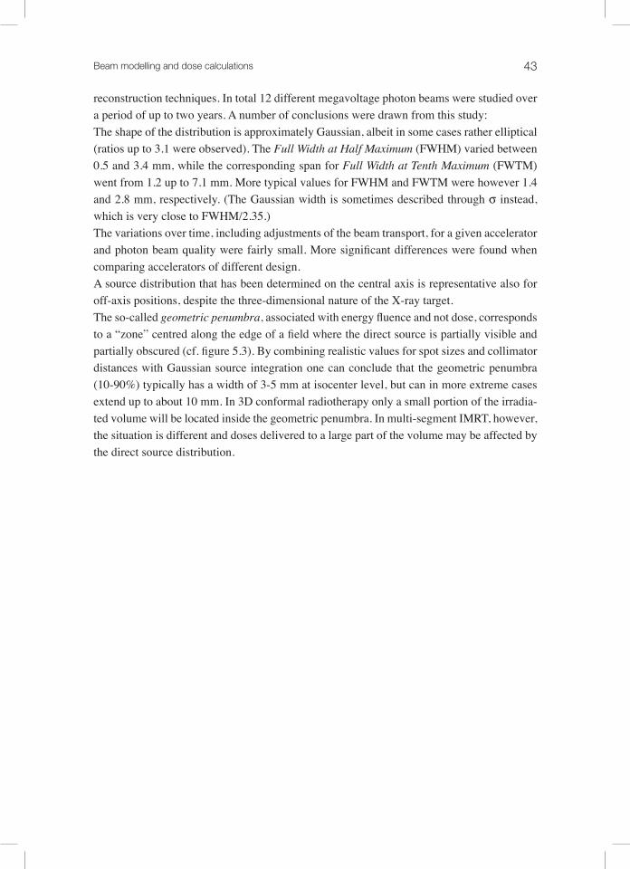
Beam modelling and dose calculations 43
reconstruction techniques. In total 12 different megavoltage photon beams were studied over a period of up to two years. A number of conclusions were drawn from this study:The shape of the distribution is approximately Gaussian, albeit in some cases rather elliptical (ratios up to 3.1 were observed). The Full Width at Half Maximum (FWHM) varied between 0.5 and 3.4 mm, while the corresponding span for Full Width at Tenth Maximum (FWTM) went from 1.2 up to 7.1 mm. More typical values for FWHM and FWTM were however 1.4 and 2.8 mm, respectively. (The Gaussian width is sometimes described through σ instead, which is very close to FWHM/2.35.)The variations over time, including adjustments of the beam transport, for a given accelerator and photon beam quality were fairly small. More significant differences were found when comparing accelerators of different design.A source distribution that has been determined on the central axis is representative also for off-axis positions, despite the three-dimensional nature of the X-ray target.The so-called geometric penumbra, associated with energy fluence and not dose, corresponds to a “zone” centred along the edge of a field where the direct source is partially visible and partially obscured (cf. figure 5.3). By combining realistic values for spot sizes and collimator distances with Gaussian source integration one can conclude that the geometric penumbra (10-90%) typically has a width of 3-5 mm at isocenter level, but can in more extreme cases extend up to about 10 mm. In 3D conformal radiotherapy only a small portion of the irradia-ted volume will be located inside the geometric penumbra. In multi-segment IMRT, however, the situation is different and doses delivered to a large part of the volume may be affected by the direct source distribution.

44
Figure 5.3. Close to the field edge the direct (focal) source is partially visible and partially obscu-red, resulting in a lateral energy fluence gradient (green curve) known as the geometric penum-bra.
The direct source distribution has, consequently, been approximated as being Gaussian in published attempts to model the geometrical penumbra explicitly through ray tracing through the treatment head (Fippel et al., 2003; Sikora et al., 2007). An alternative way of accoun-ting for the finite direct source distribution is to laterally blur the complete energy fluence distribution in the exit plane by convolution with a Gaussian kernel that corresponds to the projected source distribution in the same plane (red curve in figure 5.3). A similar approach was proposed by Ahnesjö et al (1992b) where the Gaussian blurring instead was included in the photon pencil kernel used to model the primary dose deposition. Although, in order to fully describe variations in the geometric penumbra that are associated with different colli-mators edges the process must also handle lateral variations in the size of the blurring kernel.Also well inside the beam, where the direct source is entirely visible, the lateral distribu-tion of Ψd varies somewhat. The “raw” X-ray lobe produced in the bremsstrahlung target is forward-peaked, which means that for broad beam applications it needs to be modulated in a cone-shaped flattening filter (see figure 5.2). Normally, the goal is to create a beam with a more or less uniform lateral dose distribution (Larsen et al., 1978; Olofsson et al., 2007).
dcoll
diso(SAD)
IsocenterIsoceeennnttteeeeerrrr
d
dcoll
diso(SAD)
Isocenter
Ψ
Beam modelling and dose calculations 45
The flattening filter subsequently becomes a secondary source of scattered radiation inside the treatment head (see section 5.1.2). The lateral variations in Ψd for the open portion of the beam can be derived through reconstruction of lateral dose distributions in air (Fippel et al., 2003) or in water (Ahnesjö et al., 2005; Olofsson et al., 2006a). Due to the rotational sym-metry of the flattening filter these lateral variations in Ψd are commonly described through a radial dependence, i.e. Ψd (r), in calculations.
5.1.2 extra-focal sources; flattening filter and primary collimator
Several published investigations (Jaffray et al., 1993; Sheikh-Bagheri and Rogers, 2002a; Zhu and Bjärngard, 2003) have shown that the extra-focal radiation is closely linked to the flattening filter and the fixed primary collimator (see figure 5.2). Moreover, a variety of extra-focal source distributions have previously been suggested and evaluated; conical (Ahnesjö, 1994), exponential (Hounsell and Wilkinson, 1997), polynomial (Jursinic, 1997), Gaussian (Jiang et al., 2001; Olofsson et al., 2006b), and pyramidal (Olofsson et al., 2003). Through mathematical reconstruction of measured output factors in air Zhu and Gillin (2005) deter-mined extra-focal source distributions without assuming any empirical trial function. Ah-nesjö (1994) compared calculated values of Ψe using cone-shaped, Gaussian, and flat source distributions. Although the cone-shaped source was presented as the best analytical repre-sentation of the scatter emitted by the flattening filter, the conclusion was that the shape of the source distribution is not a critical parameter due to the smoothing that is a result of the source integration procedure.The amplitude of the extra-focal source is commonly derived from output factors in air that have been measured at the isocenter point. The angular dependence in the scatter cross sec-tion and the energy loss of Compton scattered photons cause the amplitude of a fully visible extra-focal source to vary somewhat in the lateral direction. One way of modelling this, without commissioning characteristics for the extra-focal source at several positions, is to introduce multiplicative correction factors based on the beam quality and the scattering angle from the source to the calculation point (Ahnesjö, 1994). This concept was further developed by Olofsson et al (2006b), who applied a correction factor matrix on the entire extra-focal source distribution. However, a later experimental evaluation of this angular Compton cor-rection (Olofsson et al., 2006a) indicates that the effects are small enough to be ignored as it usually is balanced in fluence calculations by a lateral reduction of the direct contribution Ψd.Recently there have been publications discussing the consequences of completely removing the flattening filter from photon treatment heads (Titt et al., 2006a; Vassiliev et al., 2006). The rationale for this seemingly drastic measure is that the application of IMRT techniques ade-quately compensates for non-uniform beams. The dedicated helical tomotherapy unit (Jeraj et al., 2004) is the first commercial implementation of this idea. The associated benefits are higher dose rate, less out of field scatter, and less lateral variation in beam quality (cf. section 5.2). However, to avoid increased skin dose a thin slab filter must be used to remove low-energy particles.
46
5.1.3 physical wedge scatter
Wedges have a long tradition as beam modulators in external beam therapy. A physical wedge will, however, not only attenuate the photon beam, but also act as a source of additional pho-ton scatter (represented by Ψpw in equation (5.2)). This is one of the main reasons why the output, i.e. the fluence or dose per monitor unit, has a more pronounced field size variation for beams including a physical wedge than for open beams. Over the range of field sizes covered by the physical wedge this increase in output variation can amount to 5 or even 10% (Heukelom et al., 1994a; Zhu et al., 1995), depending on the size, thickness, and material of the wedge.An approximate source distribution for the wedge generated scatter Ψpw can be derived by setting the source intensity proportional to η⋅ln (η), where η is the beam modulation (cf. figu-re 5.4). This relation has been reported as a result of analytical (Ahnesjö et al., 1995) as well as experimental (Castellanos and Rosenwald, 1998) investigations. Consequently, the maxi-mum amount of wedge scatter will be produced when the thickness corresponds to one mean free path, i.e. η= 0.368, for a given photon beam. Furthermore, this simple concept can be combined with a range of correction factors accounting for spectral and angular effects that influence the properties of the wedge generated scatter (Ahnesjö et al., 1995). Concerning the calculation accuracy, the most problematic situations are typically associated with heavy modulation, large field sizes and/or short distances between wedge and calculation point.
a) Physical wedge modulation (6 MV photons)
0
0.2
0.4
0.6
0.8
1
-15 -10 -5 0 5 10 15Position (cm)
Mo
du
lati
on
15 deg wedge60 deg wedge

Beam modelling and dose calculations 47
Figure 5.4. As a first order approximation the scatter generated in a physical wedge (b) can be described as being proportional to η⋅ln (η), where η is the beam modulation (a). This relation is here illustrated for a 15 and a 60 degree wedge in a 6 MV photon beam (µ = 0.0507 cm-1).
In principal, a physical wedge can be mounted anywhere in the photon beam path between the focal point and the patient. In reality, however, two different designs have evolved (cf. figure 5.2); either the wedge is placed between the dose monitor chamber and the uppermost secondary collimator, known as an internal wedge, or it is placed below all the secondary col-limators, i.e. an external wedge. Internal wedges are often motorized since they can be quite hard to access manually. For an internal wedge the production of wedge scatter is indepen-dent of collimator settings, but the fraction of the scatter that reaches the patient is limited by the collimators and for a given point of interest determined by the visible parts of the wedge. For an external wedge the situation is the opposite; the wedge scatter source is always fully visible from any calculation point below the treatment head. But the source distribution itself will depend on the collimator settings above, which will limit the scattering volume of the wedge. The lack of collimation downstream from an external wedge also results in an incre-ase in scatter dose outside the beam edges (Zhu et al., 2000).
5.1.4 Collimator scatter
Among the energy fluence contributions that are included in equation (5.2) the one associated with the secondary collimators (Ψc) is generally considered to be the least significant one (Ahnesjö, 1995; Sheikh-Bagheri and Rogers, 2002a; Zhu and Bjärngard, 2003). For a typical collimator design of a linear accelerator Ψc rarely exceeds 1% of the total energy fluence.
0
15 deg wedge60 deg wedge
0
b) Physical wedge scatter (6 MV photons)
0
0.2
0.4
0.6
0.8
1
-15 -10 -5 0 5 10 15Position (cm)G
ener
ated
wed
ge
scat
ter
(rel
ativ
e u
nit
s)
15 deg wedge60 deg wedge

48
Therefore Ψc is often not modelled as an explicit part of the emitted energy fluence. Instead it is included in the extra-focal contribution Ψe (Hounsell and Wilkinson, 1996; Jiang et al., 2001; Naqvi et al., 2001), which generally works well. The collimator scatter is also more complicated to model than other secondary sources due to the simple fact that they do not have a fixed position. Furthermore, the collimating system is made up of several parts that are mounted on top of each other (see figure 5.2), which forms a scatter source that has a considerable extension along the beam direction.A straightforward approach for modelling of collimator scatter is proposed by Olofsson et al (2003), where the edges of the beam are treated as a fully visible isotropic line source. This gives Ψc proportional to the perimeter of the beam aperture and, in addition, fairly constant laterally. Inside convex beam shapes this is a valid approximation as the defining collima-tor edges are completely visible and there is, therefore, no inter-element blocking. Ahnesjö (1995) showed, however, that for focused leaves the irradiated collimator edges that face the direct source are the main contributors to Ψc. Inside a highly irregular MLC beam (like the “striped” beam in figure 5.6) or outside the beam edges considerable parts of these upper col-limator edges will be blocked by lower parts of the collimator, which consequently may lead to overestimated values of Ψc if not accounted for. An alternative way of modelling Ψc was suggested by Zhu and Bjärngard (2003) who approximated the variable collimator scatter source by a dedicated large, but static, Gaussian source that was ray traced through the col-limators located below. The calculated results were compared with measurements in air both inside and outside various rectangular beams and showed better agreement than calculations that included Ψc in the extra-focal contribution Ψe.
5.1.5 the monitor signal
The dose monitor signal M can be considered as a sum of different contributions, as indica-ted in the denominator of equation (5.2), where the direct contribution Md is the dominating part. These contributions are, with one exception, practically independent of the collimator settings. The exception is the backscattered component Mc associated with the variable se-condary collimators themselves. This component has previously been investigated through various experimental techniques and/or Monte Carlo simulations (Ding, 2004; Lam et al., 1998; Liu et al., 1997a; Verhaegen et al., 2000; Sanz et al., 2007). The reported variations in total monitor signal M over the entire range of collimator settings go from zero up to several percent. Many of the published investigations have been focused on Varian Clinac accelera-tors, and this is possibly also the major accelerator brand that is most intimately associated with considerable variations in the backscattered monitor signal (except for the GE-CGR Saturne that is no longer on the market). It has been shown that the major part of Mc is pro-duced by low-energy energy electrons (Titt et al., 2006b; Verhaegen et al., 2000). Hence, one can significantly reduce the backscatter influence by introducing a thin aluminium sheet/plate between the secondary collimators and the monitor chamber (Hounsell, 1998; Liu et al., 1997a).
Beam modelling and dose calculations 49
In a similar manner as the forward directed collimator scatter Ψc the variations in Mc have in some cases not been modelled explicitly (Hounsell and Wilkinson, 1997; Naqvi et al., 2001), which essentially means that the effect instead is treated as part of the extra-focal contribu-tion Ψe. This may constitute a source of uncertainty as a varying dose monitor signal M works as a general output correction factor, while Ψe is an additional energy fluence contribution associated with a spatial variation.yet another approach is to set the variations in Mc proportional to the irradiated collimator area facing the dose monitor chamber, but projected down to the isocenter plane (cf. figure 5.5) (Jiang et al., 2001; Lam et al., 1998). The relative importance between the different collimators can be established either empirically or by using generic relations, based on the distances between the backscattering collimator surfaces and the monitor chamber (see figure 5.2). Ahnesjö et al (1992a) proposed an inverse square relationship, while Olofsson et al (2003) set the collimator weights proportional to the inverted distances. Neither of these two relations was evaluated through explicit measurements of M or Mc, although in both cases good agreement was found between calculated and measured output factors in air.
Figure 5.5. Irradiation of collimator surfaces for a rectangular beam setting (X1, X2, Y1, Y2), as seen from the monitor chamber located upstream from the collimators. The fixed primary collimator defines a circular beam (yellow), although for simplicity the maximum square field size (green) is commonly used when calculating the backscattering areas.
x
y
X1 X2Y1
Y2
x
y
X1 X2Y1
Y2
x
y
X1 X2Y1
Y2

50
5.1.6 Collimation and ray tracing of radiation sources
In order to determine the resulting distribution of energy fluence exiting the treatment head the beam shaping process in the variable secondary collimators must be properly described. Hence, the energy fluence emitted by sources in the upper parts of the treatment head must somehow be ray traced through the structures located below (see figure 5.2). To be able to model this in a correct way the actual positions of all collimators should be known and included in the calculations. This is motivated by the fact that the view of the source plane, as seen from a point below the treatment head, actually may be defined by collimators that are retracted from the beam edges (Hounsell and Wilkinson, 1996; yu and Sloboda, 1995).A common ray tracing approximation is to employ thin collimators, i.e. collimators with no spatial extension along the beam direction. Inside fairly convex beam shapes this is a good approximation, although outside beam edges and in complex beam shapes the situation is more problematic and can lead to overestimated energy fluence contributions. An illustrative (although not clinically realistic) example of this effect is presented in figure 5.6. The pro-blem of 3D ray tracing through thick collimators can be solved analytically by calculating the traversed photon path lengths in the collimators (Chen et al., 2000; Siebers et al., 2002), which enables detailed modelling. Figure 5.6 also shows the result of extending the thin col-limator approximation to a geometry with three thin collimators, or layers, that are spread out geometrically over the full thickness of the real collimator. This simplified ray tracing through multiple discrete layers has shown good results in experimental evaluations (Naqvi et al., 2001; Olofsson et al., 2006b).
Beam modelling and dose calculations 51
Figure 5.6. The view through a “stripe field” MLC setting towards the extra-focal source, as seen from the isocenter point. A digitally enhanced photograph shows the view for a Siemens Primus accelerator, using the field light as “radiation source” (a). Applying the thin collimator ap-proximation means that the MLC is modelled through one single layer (b), but if the number of layers instead is increased to three (c) the resulting leaf projections become more similar to the real situation.
With the possible exception of so-called micro-MLCs (that can offer only a limited range of field sizes) the collimators align to the diverging beam in two different ways; either being focused, with flat front ends, or non-focused with rounded front ends. Rounded front ends typically yield beam penumbras that are broader than those associated with focused front ends, although the penumbra width depends also on the distance between the source and the collimator. The relation between the nominal and actual position of a focused collimator is trivial, provided that it is properly calibrated. For rounded collimators the situation is, ho-wever, more complex. A rounded collimator end can be positioned in relation to a diverging beam in basically three different ways (cf. figure 5.7). For a Varian type MLC, the lateral shift between projected tip and tangent alignment (A-B) increases from zero at the central
(a)
(b) (c)
(a)
(b) (c)

52
axis to roughly 3 mm at 20 cm off-axis (at isocenter distance) (Boyer and Li, 1997). The cor-responding shift between half value transmission (HVT) and tangent alignment (C-B) is on the other hand nearly constant, typically 0.3 mm. To enable accurate ray tracing it is, as previ-ously pointed out, essential to know the exact position of all collimators. The three concepts illustrated in figure 5.7 clearly indicate the need for consistency between actual collimator position during treatment delivery and modelling in TPS and IDC.
Figure 5.7. In a diverging beam the position of a rounded collimator end can be specified using three different concepts, calling for consistency between mechanical calibration, TPS, and IDC. The relations between these three positions will vary depending on the lateral position in the beam.
In order to minimize leakage between adjacent MLC leaves the leaf sides are typically sha-ped with matching tongues and grooves (Huq et al., 2002). This design will to some extent influence the beam penumbras created by the leaf sides. The most significant consequence of this design arises when a tongue or groove is matched with its counterpart in another MLC aperture. The result is a narrow stripe of reduced fluence and dose that can be attributed to the fact that the photon attenuation is not proportional to the attenuator (collimator) thickness.
A,B C CB A
A: Projected tip
B: Tangent (light field)
C: Half Value Transmission
Focal point
A,B C CB A
A: Projected tip
B: Tangent (light field)
C: Half Value Transmission
Focal point
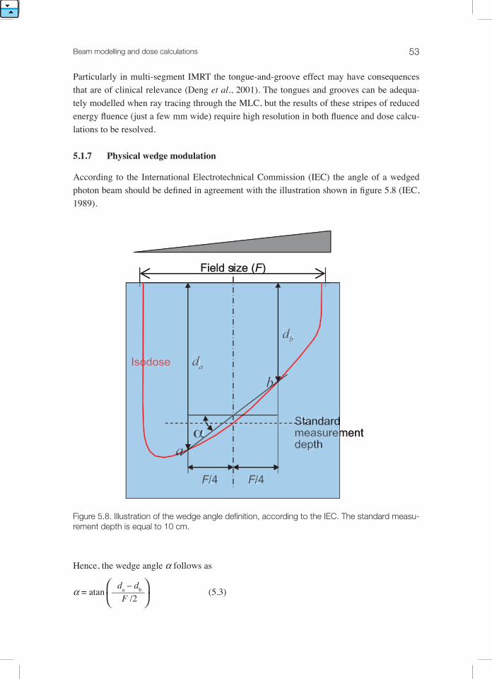
Beam modelling and dose calculations 53
Particularly in multi-segment IMRT the tongue-and-groove effect may have consequences that are of clinical relevance (Deng et al., 2001). The tongues and grooves can be adequa-tely modelled when ray tracing through the MLC, but the results of these stripes of reduced energy fluence (just a few mm wide) require high resolution in both fluence and dose calcu-lations to be resolved.
5.1.7 physicalwedgemodulation
According to the International Electrotechnical Commission (IEC) the angle of a wedged photon beam should be defined in agreement with the illustration shown in figure 5.8 (IEC, 1989).
Figure 5.8. Illustration of the wedge angle definition, according to the IEC. The standard measu-rement depth is equal to 10 cm.
Hence, the wedge angle α follows as
da – dbα = atan ––––––– (5.3) F /2
Field size (F)
F/4 F/4
Standard measurement depth
α
Isodose
a
b
da
db
F/FF 4 F/FF 4
SSStttaaandarddmeasuremmdepth
αα
Isoodose
aaa
bbb
dad
dbdd
Field size (F)
F/4 F/4
Standard measurement depth
α
Isodose
a
b
da
db

54
where da, db, and F are defined in figure 5.8. Assuming that the doses in points a and b are related to each other only through the attenuation of primary photons (i.e. neglecting any dif-ference in scatter contribution) and that the attenuation coefficient (µ) and the un-modulated energy fluence is identical in a and b, then the required ratio of beam modulation (η) between points a and b follows from
ηb -µ(da – db)
-µ·(F/2) tan·α––– = e = e (5.4)ηa
This simple relation has also been utilized to create the modulation curves for a 6 MV beam in figure 5.4(a), albeit generalizing ±F/4 from figure 5.8 to arbitrary lateral positions.Even though this simplification may be sufficient in many applications, the situation in wed-ged photon beams is in reality more complex than what is reflected in equation (5.4). The dose component originating from scattered radiation varies noticeably in the lateral direction due to the asymmetric beam profile. Furthermore, a physical wedge acts as a beam filter it-self, yielding changes in beam quality that are linked to the laterally varying wedge thickness (Tailor et al., 1998a). The modified beam quality results in altered depth doses in comparison with the corresponding open beams (Heukelom et al., 1994b, a). Another consequence of the wedge filtration is that dose profiles along the non-gradient direction are affected by the presence of a physical wedge.
5.2 dose ModellIng
The four main physical phenomena driving the formation of depth dose distributions in water are i) the inverse square law, ii) attenuation of the primary beam iii) the build-up of photon generated electron fluence (within a few cm depth) and build-up of phantom scatter dose (within 9 to 18 cm depth), and iv) electron contamination from sources in the treatment head and in the air between the treatment head and the patient. In figure 5.9 a depth dose curve is shown with the dose separated into these components. The part of the dose that is due to photons scattered in the treatment head, i.e. the indirect part of total beam fluence, is shown separately as head scatter dose. This part can also be subdivided into a primary part and a phantom scatter part, depending on how the dose calculation model treats these parts.
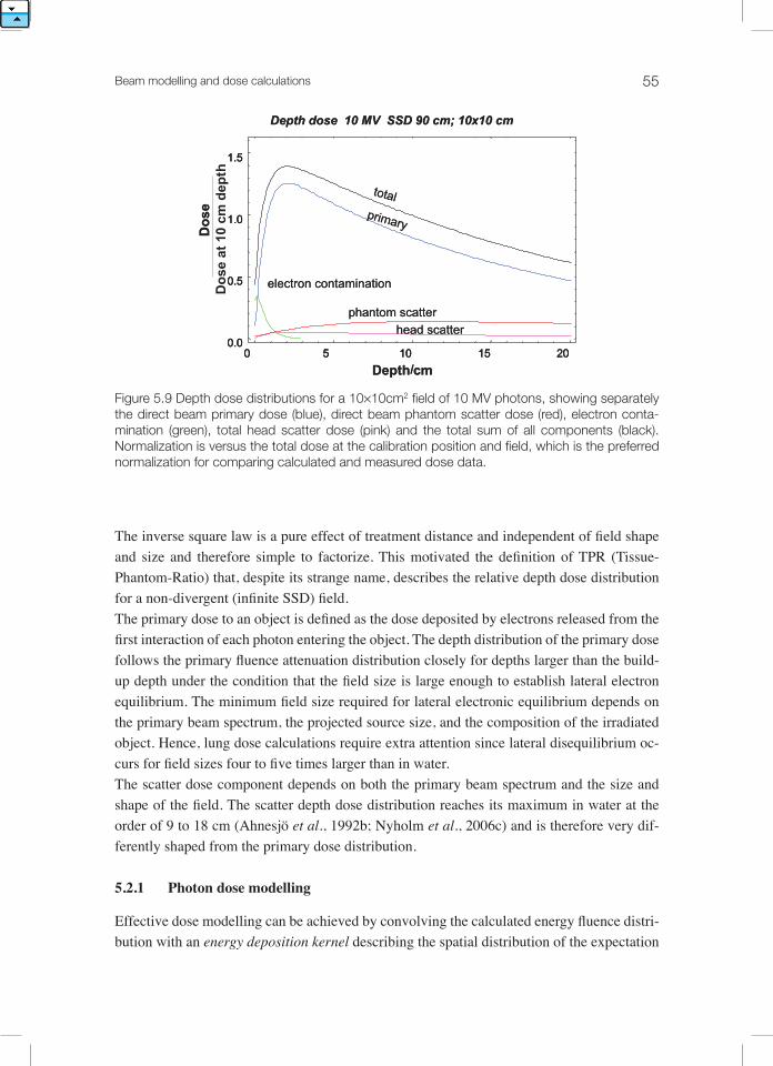
Beam modelling and dose calculations 55
Figure 5.9 Depth dose distributions for a 10×10cm2 field of 10 MV photons, showing separately the direct beam primary dose (blue), direct beam phantom scatter dose (red), electron conta-mination (green), total head scatter dose (pink) and the total sum of all components (black). Normalization is versus the total dose at the calibration position and field, which is the preferred normalization for comparing calculated and measured dose data.
The inverse square law is a pure effect of treatment distance and independent of field shape and size and therefore simple to factorize. This motivated the definition of TPR (Tissue-Phantom-Ratio) that, despite its strange name, describes the relative depth dose distribution for a non-divergent (infinite SSD) field. The primary dose to an object is defined as the dose deposited by electrons released from the first interaction of each photon entering the object. The depth distribution of the primary dose follows the primary fluence attenuation distribution closely for depths larger than the build-up depth under the condition that the field size is large enough to establish lateral electron equilibrium. The minimum field size required for lateral electronic equilibrium depends on the primary beam spectrum, the projected source size, and the composition of the irradiated object. Hence, lung dose calculations require extra attention since lateral disequilibrium oc-curs for field sizes four to five times larger than in water. The scatter dose component depends on both the primary beam spectrum and the size and shape of the field. The scatter depth dose distribution reaches its maximum in water at the order of 9 to 18 cm (Ahnesjö et al., 1992b; Nyholm et al., 2006c) and is therefore very dif-ferently shaped from the primary dose distribution.
5.2.1 photon dose modelling
Effective dose modelling can be achieved by convolving the calculated energy fluence distri-bution with an energy deposition kernel describing the spatial distribution of the expectation
Depth dose 10 MV SSD 90 cm; 10x10 cm
0 5 10 15 200.0
0.5
1.0
1.5
Depth/cm
Do
se a
t 10
cm
dep
th
total
phantom scatter
primary
head scatter
electron contamination
Do
se
Depth dose 10 MV SSD 90 cm; 10x10 cm
0 5 10 15 200.0
0.5
1.0
1.5
0 5 10 15 200.0
0.5
1.0
1.5
Depth/cm
total
phantom scatter
primary
head scatter
electron contamination
Do
se
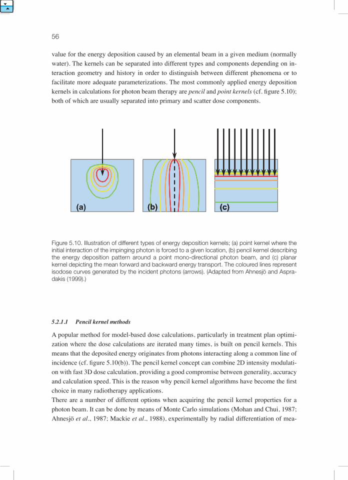
56
value for the energy deposition caused by an elemental beam in a given medium (normally water). The kernels can be separated into different types and components depending on in-teraction geometry and history in order to distinguish between different phenomena or to facilitate more adequate parameterizations. The most commonly applied energy deposition kernels in calculations for photon beam therapy are pencil and point kernels (cf. figure 5.10); both of which are usually separated into primary and scatter dose components.
Figure 5.10. Illustration of different types of energy deposition kernels; (a) point kernel where the initial interaction of the impinging photon is forced to a given location, (b) pencil kernel describing the energy deposition pattern around a point mono-directional photon beam, and (c) planar kernel depicting the mean forward and backward energy transport. The coloured lines represent isodose curves generated by the incident photons (arrows). (Adapted from Ahnesjö and Aspra-dakis (1999).)
5.2.1.1 Pencilkernelmethods
A popular method for model-based dose calculations, particularly in treatment plan optimi-zation where the dose calculations are iterated many times, is built on pencil kernels. This means that the deposited energy originates from photons interacting along a common line of incidence (cf. figure 5.10(b)). The pencil kernel concept can combine 2D intensity modulati-on with fast 3D dose calculation, providing a good compromise between generality, accuracy and calculation speed. This is the reason why pencil kernel algorithms have become the first choice in many radiotherapy applications. There are a number of different options when acquiring the pencil kernel properties for a photon beam. It can be done by means of Monte Carlo simulations (Mohan and Chui, 1987; Ahnesjö et al., 1987; Mackie et al., 1988), experimentally by radial differentiation of mea-
(a) (b) (c)(a)((aa))(( ))(a) (bb)(b)(b) (c)(c)

Beam modelling and dose calculations 57
sured scatter contributions (Ceberg et al., 1996; Storchi and Woudstra, 1996), or through deconvolution of measured dose profiles (Bergman et al., 2004; Chui and Mohan, 1988). Nyholm et al (2006c) propose a condensed characterization scheme where the beam quality index TPR20,10 is used as a single “fingerprint” to yield the complete photon pencil kernel.The pencil kernel “anatomy” must somehow be quantified in order to facilitate general dose calculations. Several proposals on how to resolve this issue can be found in the literature. Ah-nesjö et al (1992b) proposed a radial parameterization consisting of a double exponential that separates the primary and the secondary scatter contributions. Nyholm et al (2006c) utilized the same radial parameterization, although introducing a parameterization over the depth that replaced the original tabulated depth description. Alternatively, a photon pencil kernel can be described as a sum of three Gaussians (Dong et al., 1998) or by analytically differentiating parameterized scatter-primary ratios (SPRs) (Ceberg et al., 1996). yet another option is to utilize a discrete numerical description (Bergman et al., 2004), which means that the kernel has a finite spatial resolution and extension.Another issue of concern is the choice of the numerical method for lateral superposition of the pencil kernels, which is a process that must be linked to the specific pencil kernel descrip-tion. The double exponential parameterization of Ahnesjö et al (1992b) enables analytical integration over circular beams. Alternatively, arbitrary beam shapes can be decomposed into triangular beam elements that are possible to handle by so-called Sievert integrals. Both these solutions require, however, that the energy fluence be constant over each integrated area. However, non-uniform fluence distributions can be managed by fluence sampling and subsequent weighting of each surface integral before adding them together. For 2D and 3D dose calculations different fast transform convolution techniques can be utilized in order to simultaneously yield results for an entire calculation plane or volume, thereby offering considerable speedups. A commonly employed algorithm in this category is the fast Fourier transform (FFT) that enables discrete convolution of the energy fluence distribution and the pencil kernel (Mohan and Chui, 1987; Murray et al., 1989).Pencil kernel dose calculation is a compromise that in some geometries applies approxima-tions that favour simplicity and calculation speed over accuracy. One such approximation is the assumption of lateral invariance of the pencil kernel, which neglects the lateral shift in photon beam quality from off-axis softening (Tailor et al., 1998b). If this approximation is not compensated for, this may introduce dose calculations errors up to about 5% at large off-axis distances (Olofsson et al., 2006a; Piermattei et al., 1990). Furthermore, integration with laterally invariant pencil kernel parameters also implies that the depth must have a con-stant value which, in practice corresponds to a slab phantom geometry. In a situation where the depth varies considerably over the lateral plane (cf. figure 5.11) the calculated scatter contributions may, consequently, be over- or underestimated depending on the surrounding geometry (Hurkmans et al., 1995).

58
Figure 5.11. During pencil kernel integration a laterally constant depth, i.e. a slab phantom ge-ometry, is generally assumed (a). Laterally varying depths, illustrated in (b), (c), and (d), may therefore yield over- or underestimated scatter contributions, depending on the exact geometry.
Various methods to handle and correct for density variations (heterogeneities) in pencil kernel algorithms have been presented in the literature (Ahnesjö and Aspradakis, 1999). Most often these heterogeneity corrections rely on one-dimensional depth scaling along ray lines from the direct source, employing equivalent/effective/radiological depths that replace the geometrical depths in the dose calculations (cf. figure 5.12). In general, the basic concept of the pencil kernel approach, i.e. to divide the energy deposition process into separate depth and lateral components, means that the full 3D nature of the process can not be properly
Calculation point
Primary deposition volume
d
Scatter overestimated
(b)
Calculation point
Primary deposition volume
d
Scatter underestimated
(c)
Errors cancel (roughly)
Calculation point
Primary deposition volume
d(d)
Calculation point
Primary deposition volume
d(a)
Homogeneousslab phantom
Calculation point
Primary deposition volume
d
Scatter overestimated
(b)
Calculation point
Primary deposition volume
d
Scatter overestimated
(b)
Calculation point
Primary deposition volume
d
Scatter underestimated
(c)
Calculation point
Primary deposition volume
d
Scatter underestimated
(c)
Errors cancel (roughly)
Calculation point
Primary deposition volume
d(d)
Errors cancel (roughly)
Calculation point
Primary deposition volume
d(d)
Calculation point
Primary deposition volume
d(a)
Homogeneousslab phantom
Calculation point
Primary deposition volume
d(a)
Homogeneousslab phantom

Beam modelling and dose calculations 59
modelled. The result is that all deviations from the ideal slab phantom geometry, either by external shape or internal composition of the irradiated object, will cause different errors in the calculated doses.
Figure 5.12. If the density variations (heterogeneities) fit the slab phantom geometry (a) pencil kernel models can yield fairly correct dose calculations through the use of an equivalent depth, here denoted deq. However, scatter effects associated with heterogeneities that are smaller than the lateral beam dimensions, illustrated by a low-density volume ρ1 in (b), (c), and (d), can not be adequately modelled. In addition, the primary dose deposition is generally not scaled laterally, which means that it will be incorrectly modelled in cases of lateral charged particle disequilibrium (d).
Calculation point
Primary deposition volume(c)
deqρ0
ρ1
Scatter underestimated
Heterogeneousslab phantom
Calculation point
Primary deposition volume(a)
deqρ0
ρ1
Calculation point
Primary deposition volume(b)
dρ0 ρ1
Scatter overestimated
Calculation point
Primary depositionvolume(d)
dρ0 ρ1
Scatter and primary overestimated
Calculation point
Primary deposition volume(c)
deqρ0
ρ1
Scatter underestimated
Calculation point
Primary deposition volume(c)
deqρ0
ρ1
Scatter underestimated
Heterogeneousslab phantom
Calculation point
Primary deposition volume(a)
deqρ0
ρ1
Heterogeneousslab phantom
Calculation point
Primary deposition volume(a)
deqρ0
ρ1
Calculation point
Primary deposition volume(b)
dρ0 ρ1
Scatter overestimated
Calculation point
Primary deposition volume(b)
dρ0 ρ1
Scatter overestimated
Calculation point
Primary depositionvolume(d)
dρ0 ρ1
Scatter and primary overestimated
Calculation point
Primary depositionvolume(d)
dρ0 ρ1
Scatter and primary overestimated
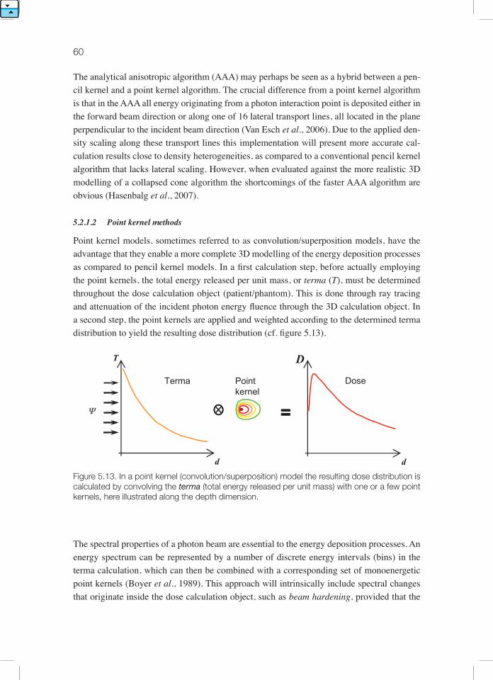
60
The analytical anisotropic algorithm (AAA) may perhaps be seen as a hybrid between a pen-cil kernel and a point kernel algorithm. The crucial difference from a point kernel algorithm is that in the AAA all energy originating from a photon interaction point is deposited either in the forward beam direction or along one of 16 lateral transport lines, all located in the plane perpendicular to the incident beam direction (Van Esch et al., 2006). Due to the applied den-sity scaling along these transport lines this implementation will present more accurate cal-culation results close to density heterogeneities, as compared to a conventional pencil kernel algorithm that lacks lateral scaling. However, when evaluated against the more realistic 3D modelling of a collapsed cone algorithm the shortcomings of the faster AAA algorithm are obvious (Hasenbalg et al., 2007).
5.2.1.2 Pointkernelmethods
Point kernel models, sometimes referred to as convolution/superposition models, have the advantage that they enable a more complete 3D modelling of the energy deposition processes as compared to pencil kernel models. In a first calculation step, before actually employing the point kernels, the total energy released per unit mass, or terma (T), must be determined throughout the dose calculation object (patient/phantom). This is done through ray tracing and attenuation of the incident photon energy fluence through the 3D calculation object. In a second step, the point kernels are applied and weighted according to the determined terma distribution to yield the resulting dose distribution (cf. figure 5.13).
Figure 5.13. In a point kernel (convolution/superposition) model the resulting dose distribution is calculated by convolving the terma (total energy released per unit mass) with one or a few point kernels, here illustrated along the depth dimension.
The spectral properties of a photon beam are essential to the energy deposition processes. An energy spectrum can be represented by a number of discrete energy intervals (bins) in the terma calculation, which can then be combined with a corresponding set of monoenergetic point kernels (Boyer et al., 1989). This approach will intrinsically include spectral changes that originate inside the dose calculation object, such as beam hardening, provided that the
=
Point kernel
d
D
Dose
d
T
Terma
Ψ ==

Beam modelling and dose calculations 61
number of bins is adequate. The drawback is that the terma calculation and the point kernel superposition must be repeated for each energy bin employed, resulting in long calculation times. The use of a single poly-energetic point kernel will speed up the superposition consi-derably, although the requirement to model the spectral variations over the dose calculation volume remains. One solution to this problem is to combine two different polyenergetic point kernels; one associated with the primary dose deposition and one with the scatter dose depo-sitions (Hoban, 1995; Ahnesjö, 1991). The terma should at the same time be divided into two corresponding components; the collision kerma (Kc) and the scatter kerma, or scerma, (S)
μenKc (s) = ∫ TE(s) ––– (E) dE (5.5) μ
μenS (s) = ∫ TE(s) 1 – ––– (E) dE (5.6) μ
Hence, Kc and S are determined by weighting the ratios of µen and µ in agreement with the energy spectrum at the photon interaction site s, including effects that originate both inside and outside the calculation object (such as the off-axis softening). Through Kc and S a two-fold point kernel superposition procedure is enabled that provides accurate dose modelling throughout the calculation volume.Energy deposition modelled by means of point kernels generally includes scaling along dis-crete and straight lines joining the primary photon interaction site and the energy deposition points. Consequently, the applied density scaling is only affected by the media encountered along these straight lines. While exact for the first scatter component, the scaling of the mul-tiple scatter is approximate (Ahnesjö and Aspradakis, 1999). Inside a large homogeneous phantom, similar to where the point kernel originally was created, this is not a problem as long as the resolution of the kernel superposition is properly set. However, in a heterogene-ous calculation object the multiple scattered particles may encounter other media, possibly not present at all along the straight transport line. The situation is similar close to outer boundaries where the use of a kernel derived inside an infinite phantom will result in overes-timated doses due to missing multiple scatter. In fact, for a given point in an irradiated object there is one unique kernel “anatomy” that perfectly describes the energy deposition stem-ming from that point (Woo and Cunningham, 1990). Various methods have been proposed to reduce the effects of the linear energy deposition approximation (Keall and Hoban, 1996; Yu et al., 1995), all associated with increasing calculation times. However, the total dose at a point is the sum of contributions from all surrounding interaction points, implying that errors related to inadequate modelling of multiple scatter from a few directions will be less critical when added together with all the other contributions. To maximize the calculation accuracy, tilting the point kernels due to the geometric beam divergence should also be included in the algorithm (Liu et al., 1997b). In essence, despite the restriction to only transport energy in straight lines between the photon interaction and dose deposition sites, point kernel based
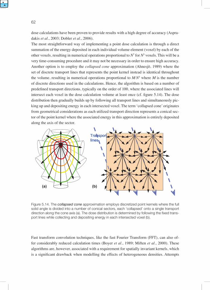
62
dose calculations have been proven to provide results with a high degree of accuracy (Aspra-dakis et al., 2003; Dobler et al., 2006).The most straightforward way of implementing a point dose calculation is through a direct summation of the energy deposited in each individual volume element (voxel) by each of the other voxels, resulting in numerical operations proportional to N7 for N3 voxels. This will be a very time-consuming procedure and it may not be necessary in order to ensure high accuracy. Another option is to employ the collapsed cone approximation (Ahnesjö, 1989) where the set of discrete transport lines that represents the point kernel instead is identical throughout the volume, resulting in numerical operations proportional to M⋅N3 where M is the number of discrete directions used in the calculations. Hence, the algorithm is based on a number of predefined transport directions, typically on the order of 100, where the associated lines will intersect each voxel in the dose calculation volume at least once (cf. figure 5.14). The dose distribution then gradually builds up by following all transport lines and simultaneously pic-king up and depositing energy in each intersected voxel. The term ‘collapsed cone’ originates from geometrical considerations as each utilized transport direction represents a conical sec-tor of the point kernel where the associated energy in this approximation is entirely deposited along the axis of the sector.
Figure 5.14. The collapsed cone approximation employs discretized point kernels where the full solid angle is divided into a number of conical sectors, each ‘collapsed’ onto a single transport direction along the cone axis (a). The dose distribution is determined by following the fixed trans-port lines while collecting and depositing energy in each intersected voxel (b).
Fast transform convolution techniques, like the fast Fourier Transform (FFT), can also of-fer considerably reduced calculation times (Boyer et al., 1989; Miften et al., 2000). These algorithms are, however, associated with a requirement for spatially invariant kernels, which is a significant drawback when modelling the effects of heterogeneous densities. Attempts
(a) (b)
Transport lines
tnTransport lines
Beam modelling and dose calculations 63
have been made to compensate for this limitation by scaling the calculated dose distribution, or at least the scattered component, by the density at the scattering and/or the deposition site (Boyer and Mok, 1986; Wong et al., 1996; Wong and Purdy, 1990). The resolution of the dose calculation grid is yet another parameter that can be explored in order to reduce calculation times. Miften et al (2000) implemented a collapsed cone algorithm where the gradients of energy fluence and density in the beam and in the dose calculation object, respectively, were used to vary the resolution of the calculation grid over the volume. During the collapsed cone calculation every other point was omitted in low gradient areas and the missing doses were then determined later on through interpolation. On average this reduced the calculation time by a factor of 3.5 without leading to any noticeable reductions in calculation accuracy. Ano-ther approach that offers considerable speedups is to perform a point kernel calculation on a very coarse calculation grid that is only to be used as a 3D correction factor for a simpler and faster dose calculation algorithm performed on a fine grid (Aspradakis and Redpath, 1997).
5.2.2 Charged particle contamination modelling
High-energy photon beams delivered by medical linear accelerators should not be regarded as pure photon beams as they are in fact contaminated by charged particles, essentially elec-trons and to some extent positrons that contribute significantly to the dose in the build-up region (fig 5.9). The origin of these electrons can be found inside the treatment head, most often in the flattening filter or the dose monitor chamber (see figure 5.2), and in the irradiated air column (Petti et al., 1983). At higher beam energies the treatment head is typically the dominating source of contaminant electrons, while the electrons generated in air gain impor-tance with decreasing beam energy (Biggs and Russell, 1983). Monte Carlo simulations have shown that the energy spectrum of contaminant electrons in a megavoltage photon beam has a similar shape as the spectrum of primary photons (Sheikh-Bagheri and Rogers, 2002a). The continuous distribution of electron energies yields depth dose characteristics that can be adequately described by an exponential curve (Beauvais et al., 1993; Sjögren and Karlsson, 1996), which is noticeably different from depth dose curves associated with clinical elec-tron beams. The lateral distribution of dose from contaminant electrons has been reported as being rounded, i.e. more intense in the central parts of the beam (Nilsson, 1985; yang et al., 2004). Also the collimator opening and the treatment distance (SSD) have been shown to be important parameters to consider when trying to quantify the dosimetric significance of charged particle contamination in different treatment situations (Sjögren and Karlsson, 1996; Zhu and Palta, 1998).To model the charged particle contamination in dose calculations Ahnesjö et al (1992b) se-parated the dependence into a lateral Gaussian pencil kernel and an exponentially decrea-sing depth dose. The Gaussian kernel is characterized by its width parameters, which can be derived through comparison of calculated depth dose curves associated with a (theoretical) pure photon beam and corresponding measurements in the (real) contaminated beam. Fip-pel et al (2003) and yang et al (2004) have both presented multi-source models intended for

64
Monte Carlo purposes that include a separate circular electron contamination source located in the upper parts of the treatment head. The pencil kernel correction derived empirically by Nyholm et al (2006a) will largely compensate at shallow depths for charged particle con-tamination, which was not included in the original kernel parameterization (Nyholm et al., 2006b, c).
5.3 patIent representatIon
The actual geometry of the dose modelling object, i.e. the patient, is often not included when independently verifying the dose calculations for a treatment plan. One explanation for this may be that no appropriate modelling of the full patient geometry is facilitated by the factor based methods traditionally employed for IDC. Furthermore, applying some sort of standar-dized dose modelling object simplifies the verification process as it eliminates the require-ment to import a CT-study, define patient contours, etc. for each individual treatment plan. The minimum information to perform calculations for arbitrary beams on a standardized dose modelling object can be restricted to its position and rotation (for a finite 3D phantom) or just the SSD (for an infinite slab phantom with its surface perpendicular to the beam central axis).The fact that the conditions applied in the IDC-verified plan are usually not identical to the dose calculations in the treatment plan can be somewhat problematic to handle. One option is to repeat the dose calculations in the TPS after replacing the patient by the standardized dose modelling object from the IDC. This method should, consequently, yield identical cal-culation results and enable a detailed comparison. This approach is frequently employed for experimental verification where a detector, e.g. an ionization chamber, is positioned inside an irradiated QA phantom and the measured dose is then compared with a corresponding calculation from the TPS. Even if the actual patient geometry in this case is absent in the IDC tool, all characteristics of the energy fluence that exits the treatment head are still included. A drawback is, however, that the extra dose calculation that must be carried out in the TPS imposes an additional workload.Another alternative, perhaps more frequently applied, is to accept that the dose modelling object in the IDC is different from the TPS calculation. This also means that one must be pre-pared to find and accept deviations that are caused by these differences. Obviously this adds significant uncertainty to the QA procedure as it requires the ability to distinguish between deviations associated with the dose modelling object and deviations that are related to actual flaws/bugs in the calculations. Typical sources of deviations due to the non-identical dose modelling objects are heterogeneities and irregular outer boundaries of the patient (Mijn-heer and Georg 2008). The irregular shape can affect both the calculation depths and the lateral size of the scattering volume inside the beam (so-called ‘missing tissue’). In order to compensate for the major sources of uncertainty in the IDC an equivalent/effective/radiolo-gical depth is regularly applied, yielding dose deviations that in most cases are within a few percent. These modified depths are generally provided by the TPS, which is a practice that
Beam modelling and dose calculations 65
should be questioned as it also compromises the independence of the two dose calculations. But from a practical point of view it may be difficult to derive them in some other way by simple means.
5.4 CalCulatIon unCertaIntIes
Over the years a number of publications have addressed the clinical requirements for dosime-tric accuracy in radiotherapy (Brahme et al., 1988; ICRU, 1976; Mijnheer et al., 1989, 1987) and the general conclusion seems to point to the interval between 3 and 5% expressed as 1 SD in the dose specification point. Ahnesjö and Aspradakis (1999) tried to identify the accuracy goals that should be associated with dose calculations in radiotherapy by combining estima-ted uncertainties in absolute dose calibration (Andreo, 1990) with a corresponding estimate for the clinical dose delivery (Brahme et al., 1988). Using these input data the conclusion was that if the dose calculation uncertainty, corresponding to one standard deviation, is larger than 2-3% it will seriously affect the overall dosimetric accuracy. Since then the estimated uncertainty for absolute dose calibration in high-energy photon beams has improved from 2.0 to 1.5% (IAEA, 2000a), implying that the scope for “imperceptible” dose calculation uncertainties also has decreased somewhat. Furthermore, by reducing the other uncertainties to account for future developments, it was concluded that as an ultimate design goal the uncertainties that are associated with dose calculation methods in radiotherapy should be limited to 1% (1 std. dev.). Note that in order to avoid ambiguity all uncertainties should be clearly specified.Uncertainties that are associated with dose calculation models employed in radiotherapy are in general not systematically accounted for in clinical procedures, as discussed in chapter 3. The main reason for this is simply that they are not clearly presented and are, therefore, not readily available to clinical users. Most scientific publications dealing with dose calculation algorithms contain some kind of basic analysis of discovered deviations and uncertainties. But the implications of these findings are rarely brought forward, discussing how the infor-mation can be transferred and made useful in the clinical situation. To better incorporate esti-mated uncertainties in dose calculations into clinical use the uncertainties should be presen-ted together with the calculation results, preferably individualized with respect to the specific setup. Such an approach requires that a separate model be created that can adequately predict the calculation uncertainty for any given treatment situation.There are published attempts to find models capable of estimating the dose calculation uncertainty in individual treatment setups. Olofsson et al (2003; 2006b) analyzed deviations between calculations and measurements of output factors in air, which resulted in a simple empirical model based on square summation of discrete uncertainty components. Thus, the validity of this model relies on the assumption that these components, associated with tre-atment parameters such as beam shape, treatment distance etc., are independent from each other. By utilizing a database consisting of measured beam data from 593 clinical mega-

66
voltage photon beams Nyholm et al (2006a) managed to extract both an empirical pencil kernel correction and a model for estimation of the residual errors linked to the pencil kernel properties. By combining the models of Olofsson et al and Nyholm et al the calculation uncertainties associated with the total dose output, i.e. dose per MU, have also been estimated (Olofsson et al., 2006a; Olofsson et al., 2006b). Even though the results indicate that this is a feasible concept, it is rather difficult to judge the validity of such uncertainty predictions. The statistical nature of the problem requires the use of extensive data sets during evaluation in order to achieve acceptable significance. Another issue that must be considered is the accuracy of the reference values themselves, i.e. the dose measurements, if the uncertainty estimations are evaluated by empirical means. All measurements are associated with some kind of experimental uncertainty that will become part of the evaluation procedure as well, if not somehow explicitly accounted for. Another option for evaluating such models of uncer-tainty estimation would be to replace the measured references by equivalent Monte Carlo simulations that are able to present a similar degree of accuracy. The possibilities offered by a Monte Carlo simulation package in terms of beam parameter configuration etc. would also enable a more detailed investigation of the reasons behind the encountered dose calculation uncertainties.As a general remark, it is important to evaluate and understand the uncertainties introduced in the individual steps of the treatment process and how they combine to the total uncertainty in the actual treatment. For instance, how will simplifications in the patient geometry or use of a more approximate dose model affect the total uncertainty in different types of treatments? There is no general answer to this question but if the analysis is performed and the more ad-vanced methods are applied only where needed, a lot of extra work may be saved while still keeping tight dosimetric tolerance limits. In this analysis one must also keep in mind that use of more advanced methods may also increase the uncertainty due to user errors which under some circumstances may contribute significantly to the total uncertainty.
67
6. Measured data For verIFICatIon and dose CalCulatIons
All dose calculation methods use experimental data to characterize the radiation source(s) into sufficient detail. These data must be expressed in quantities suitable to the algorithm, or processed into such quantities. Early dose calculation models were designed to use measured dose distribution data directly through simple factorisation. Then data could then be applied to different clinical beam geo-metries for simpler treatment techniques. Several detailed formalisms have been worked out to consistently define factors to cover possible clinical cases as completely as possible (Das et al., 2008a; Dutreix et al., 1997). Beam data used in these older dose calculation models was primarily directed towards determination of the absorbed dose distributions in a phantom, rather than to find methods for determination of emission characteristics such as the source distribution, source intensity and energy spectra that cause the observed dose distribution. Even though these older models are sufficient for treatments using simple fields this approach becomes very impractical for the more general radiation conditions encountered in advanced technologies such as IMRT that more fully exploit the degrees of freedom offered by modern radiotherapy hardware. The most fundamental approach to model a treatment field would be to describe the electron source of a treatment unit in differential terms of position, energy and angle, and use trans-port calculations based on a complete geometrical description of the treatment head. This approach has been extensively utilized for researching beam properties by means of Monte Carlo transport calculations (Rogers et al., 1995), but for most practical cases in clinical dose calculations one must use more efficient methods, e.g. parameterized multi-source models. In the latter approache the beam is modelled by combining source emission distributions with a geometrical description of the source. Further, shielding and scatter of the emitted fluence from the source is simulated. Modelling of several radiation sources is needed to describe the effects from both the primary beam source and major scattering elements like the flattening filter. The sources need to be parameterized as extended sources rather than point sources to model effects like geometrical penumbra and head scatter variations. Hence, use of a multi-source approach as implemented in a TPS or an IDC code requires determination of the parameters needed to model the sour-ces. Given a very detailed description of the treatment head design, a fundamental approach with full transport calculations through the treatment head can be used to yield phase space sets of particles exiting the machine. These sets can then be back-projected to the source planes, and tallied for parameterization with respect to at least energy and position (Fix et al., 2001). In applying this approach measured data are needed mainly for verification purposes. Even though the concept in principle is simple, applying this approach in practice requires fa-miliarity with Monte Carlo or similar calculation techniques that might not be available in the clinic. Also, detailed information about the geometrical details of the treatment head might

68
be cumbersome to access and verify. However, in future it is likely that new machines will be delivered with complete source parameterization derived through this kind of procedure. A practical approach is to derive the source parameters through minimization of deviations between measured and calculated dose data while varying the source parameters (Ahnesjö et al., 2005; Bedford et al., 2003; Fippel et al., 2003; Olofsson et al., 2003). Commonly the TPS and IDC systems employing this kind of models provide support or software tailored for this purpose. The optimization procedure has also the benefit of biasing the parameters towards the intended end result, and will also give an estimate of the expected performance of the calculations. The input data to this type of software consists of measured dose data and geometrical descriptions of the machine into some detail depending how explicit the dose calculation system will model collimating effects such as “tongue and groove” effect, leakage through rounded leaf tips, etc. The required level of detail is generally less than for a full transport calculation. Independent of the applied method, any error in the measured input data will result in para-meter errors that will degrade the overall calculation accuracy. The intention of this chapter is to briefly discuss possible measurement issues in relation to the final accuracy of the dose calculations. For more in depth details of measurement and beam commissioning procedures the reader is referred to report from the AAPM taskgroup 106 (Das et al., 2008a).
6.1 IndependenCe oF Measured data For dose verIFICatIon
With similar types of dose calculation algorithms in a clinic’s TPS and IDC, both systems could in theory be commissioned with identical data sets. However, due to the lack of standards for specifying and formatting dosimetric data for such systems the TPS and the IDC will probably require different, system-specific data sets. Although reformatting and interpolation methods might enable transformation of data sets from one system to another, this is not recommended for IDC verification as an error in the TPS data thus may cause cor-related errors in the transformed IDC data set. The risk for correlated errors can be further reduced if the IDC and the TPS use completely different type of beam data.The absolute dose calibration is performed in the reference geometry, and to establish the dose per monitor unit any IDC-TPS combination will use the same calibration geometry which thus will be an identical data entity in both systems. However, the validity of this absolute dose calibration should be checked through other QA procedures like independent reviewing and periodic verification measurements.

69Measured data for verification and dose calculations
6.2 treatMent head geoMetry Issues and FIeld speCIFICatIons
In addition to measurable dosimetry data, multi-source models need a geometrical descrip-tion of the treatment head with enough details to correctly describe the variation of source effects. This type of data consists of both field independent data like the locations of filters and collimators, as well as field dependent data like collimator settings. The latter data are normally accessible in DICOM format through treatment plan databases. It is of immense importance that the DICOM format field specifications from the TPS are correctly execu-ted on the treatment machine. If not, inconsistencies in auxiliary beam set up may lead to unexpected deviations between the calculated and delivered dose. This must be verified by an independent QA procedure, at least when hardware or software modifications have been made to the accelerator or the TPS.Use of rounded leaves is another issue that may cause inconsistencies in field size specifica-tions since the positions of the leaf tip projection and the radiation field edge differs syste-matically, see figure 5.7 (Boyer and Li, 1997; Boyer et al., 2001). Especially for small field dosimetry of narrow slit IMRT the leaves must be positioned with high accuracy since small errors in leaf positioning amplify into large errors in delivered dose (Kung and Chen, 2000; Cadman et al., 2002; Das et al., 2008b).
6.3 depth dose, tpr and beaM QualIty IndICes
In most dose calculation systems the dose component related to contaminating electrons on the surface is often less accurately modelled than other dose components. This electron con-tamination may also introduce errors in output measurements. It has a complex dependence on radiation field geometry and direct beam energy since any irradiated accelerator part will release electrons and positrons that may travel far in air and can be scattered considerably. The maximum penetration depth of these particles is determined by the most energetic elec-trons and may thus well exceed the dmax-depth. This must be considered when selecting build-up caps for head scatter measurements. By using a well specified field size it is possible to obtain attenuation measurements that cor-relate well with various spectrum-dependent quantities. This is the basis for the construction of beam quality indices like TPR20/10 and %dd10 (Andreo, 2000; Rogers and yang, 1999). These indices were originally designed as surrogates for the full spectrum to facilitate tabu-lation of pre-calculated values of water-to-air stopping power ratios for absolute dosimetry, but have also been applied for parameterization of energy deposition kernels (Nyholm et al., 2006c) and scatter factors (Bjärngard and Petti, 1988; Bjärngard and Vadash, 1998). Energy deposition kernels such as pencil kernels or point kernels are used by many dose calculation systems. The kernels are based on spectrally dependent data for which the qua-lity of measured depth dose data can be of crucial importance. The most direct approach for
70
derivation of pencil kernel data is to differentiate TPR tables with respect to field radii for circular fields (Ceberg et al., 1996). In such applications, it is practical to use the relation R = 0.5611 S to calculate the radius R of the circular field that gives the same dose on the cen-tral axis as a square field of side S (Tatcher and Bjärngard, 1993). A more explicit procedure is to determine the spectrum from depth dose data for one or several field sizes by automated optimization (Ahnesjö et al., 2005; Ahnesjö and Andreo, 1989), or manual trial (Starkschall et al., 2000), and use the spectrum for superposition of pre-calculated Monte Carlo mono-energetic kernels. This approach needs constraints to achieve a physically realistic shape of the spectrum since separation of depth data into spectral components is highly uncertain due to the weak energy dependence of the beam attenuation (Ahnesjö and Andreo, 1989; Sauer and Neumann, 1990). A robust method to obtain pencil kernel data has been demonstrated by a number of investi-gators (Nyholm et al., 2006a; Nyholm et al., 2006b, c) who used a database of parameterized kernels for a large set of treatment machines and correlated those to beam quality index, resulting in a direct mapping of beam index to pencil kernels for the accelerator designs in common use (60Co beams and treatment machines without flattening filters were not included in the study). Since the only data needed were the beam quality index, no depth dose data or output factors needed to be fitted, making the method very effective for routine use. Once the quality index is known for a particular machine, the method can also be used for consistency checks of measured depth doses by comparing with calculated depth doses. Whatever depth dose data are needed by the dose calculation algorithm, the outcome depends on the data acquisition integrity. The measurement technique for depth dose is often simpler and more reliable than for TPR if a suitable scanning water phantom is available. If TPR data are required they can be recalculated from the depth dose data and vice versa, (Purdy, 1977; Das et al., 2008a). Erroneous measured data may seriously corrupt the dose calculations. The nature of these er-rors may range from direct replication of measured dose errors to offset of model parameters with serious effects that may appear uncorrelated to its cause. As an example, if depth dose is used to unfold the beam spectrum, a depth offset can be interpreted as increased beam pe-netration, yielding a spectrum with higher mean energy, which then reduces both attenuation and scatter. A simple check may be performed however, as depth dose curves normalized per monitor unit and plotted together for different field geometries, can never cross each other since the scatter dose increases with field area for all depths.In the build-up region, care should be taken since the normally used effective point of measu-rement for cylindrical ionization chambers is derived for the conditions valid only at depths larger than the depth of dose maximum. The build-up is a high gradient region where the size of the detector is critical and small detectors such as diodes or pinpoint chambers are prefer-red. A further concern is the high presence of electron contamination in the build-up region which will vary significantly with field settings. This contribution is included in the dose
71Measured data for verification and dose calculations
calculation by various models (chap. 5.2) which should be considered in the measurement situation as these models may require different datasets. The spectral properties of primary and scattered photons are different, which can cause pro-blems with detectors such as diodes which typically over respond to low-energy photons. This is a particular problem in large photon fields where a large fraction of the photons are scattered, thus yielding a high abundance of low energy photons. yet another set of problems arises for small fields where the penumbras from opposing field edges overlap in the centre of the field. Scanning of depth dose and transversal profiles in such fields requires particular concern when aligning the scan path with the beam centre. The size of the detector is also critical and must be small enough to adequately resolve the dose variations in the beam.
6.4 relatIve output MeasureMents
The absolute dose calibration is normally performed to give a standard dose per monitor unit in a well defined standard geometry, in the normal case 1 Gy per 100 MU. The relative output (Scp) is then defined as the ratio of the dose per monitor unit at a reference point in a field of interest to the dose per monitor unit for the same point in the reference field. If the relative output data should be used in a fluence model for the treatment head connected to a dose model for the resulting dose distribution in an object, the output measurements must be acquired following specific procedures. These procedures must differentiate between scat-ter originating from the treatment head (Sc), that influences the photon fluence per monitor unit, and scatter originating in the irradiated object (Sp) that influences the resulting dose per incident energy fluence.
6.4.1 head scatter factor measurements
Through the use of a phantom small enough to be entirely covered by all intended fields, measured output factors then map the field size dependence of the energy fluence output and its in energy absorption characteristics of the phantom medium. The factor relating this to the reference conditions has been given different names such as output in-air, head scatter factor, or collimator scatter factor. These respective names reflect the process of measuring with small phantoms in air, that the source of variation is mainly the scattering processes in the treatment head, and that changing collimator settings is the clinical action causing the varia-tions. Measurements of this factor for field A are done versus a reference setup Aref, normally a 10x10 cm2 field, with the detector at the isocenter:
Signalsmall phantom (A)/MSc (A) = ––––––––––––––––––––––––––– . (6.1) Signalsmall phantom (Aref)/M @isocenter
72
When using diodes for small field measurements the use of a smaller reference field (5x5 cm2) is recommended to reduce influence from low energy scatter (Haryanto et al., 2002). However, data should for presentation be renormalized to the customary 10x10 cm2 field perhaps by using ionization chamber data to avoid confusion. The most critical issue is to ensure that the contaminant electrons and positrons do not give rise to any perturbing signal. The penetration distance indicates how thick a build-up cap must be to stop enough of these particles from reaching the detector volume while measuring head scatter factors. The proto-col recommended by ESTRO in 1997 (Dutreix et al., 1997) applied a plastic mini-phantom. The dimensions of that phantom however were too large to permit field sizes smaller than 5x5 cm2. Li et al (1995) determined the radial thickness required to establish lateral electron equilibrium to r = (5.973 TPR20,10 - 2.688). For a typical 6 MV beam with TPR20,10 = 0.68, this translates into a water equivalent thickness of 14 mm. They also claimed that brass caps can be used without serious energy response alterations. Weber et al (1997) recommended use of brass caps with a rule of thumb thickness MV/3 expressed as g cm-2. For a 6 MV beam this implies 20 mm water equivalent thickness which with brass of density 8.4 g cm-3 translates to 2.5 mm bulk thickness thus enabling measurements in small fields. For large fields a small energy dependence with brass caps was also noted due to the lower energy of the head scat-tered photons. This effect was shown to increase with higher beam energies. Furthermore, the filtration of metal wedges affects the energy spectrum of the beam. The wedge factors should therefore not be measured with brass caps as the energy change due to filtration may alter the response dosimetry system. For practical use, brass caps of thicknesses following the rules of thumb given above could be used for small fields. For high-accuracy measurements in larger fields the brass caps should be replaced by build up caps of lower atomic number, where the lower density and hence larger size is not a problem.
6.4.2 total output factors
Contrary to the situation for head scatter factors, the use of a phantom larger than all inten-ded fields causes the measured output to quantify the combined effects of energy fluence per monitor unit variations and field-size specific scatter buildup in the phantom. This quantity is defined as the total output factor, Scp. For standard fields, large enough to provide lateral char-ged particle equilibrium over an area large enough to cover the detector, the measurements can be done by common techniques according to the definition;
Dwater phantom (A)/MScp (A) = ––––––––––––––––––––––– . (6.2) Dwater phantom (Aref)/M @isocenter
Extending the scope of measurements to the small field domain and IMRT verification in-volving high gradients requires the use of small detectors carefully selected with respect to their characteristics (Zhu et al 2009). Since small field output factors may be requested by the
73Measured data for verification and dose calculations
dose calculation model to establish the effective source size for calculations in high gradient regions, all such data should be checked with respect to calculation consistency.
6.4.3 phantom scatter factors
Phantom scatter factors, Sp, can be obtained by several different methods. By cutting phant-oms to conform to the beam shapes and irradiating these with fully open beams, with all collimators withdrawn, one creates radiation conditions for which the variation of scatter dose with field size can be determined. Since this procedure is experimentally impractical it is instead customary to estimate the phantom scatter through
ScpSp = –––– . (6.3) Sc @isocenter
It is important to keep in mind that Eq. (6.3) is an approximation and not the definition of phantom scatter factor since the distribution of head scatter photons is not limited by the no-minal field size but has a more Gaussian shape within the field. The fraction of the phantom scatter generated by photons scattered in the treatment head will thus be slightly different from the contribution from primary photons which are properly collimated. Instead of being measured, the phantom scatter variation with field size can be calculated from parameterizations of standard data based on the beam quality index as outlined by se-veral groups (Storchi and van Gasteren, 1996; Venselaar et al., 1997; Bjärngard and Vadash, 1998; Nyholm et al., 2006c). This provides a route for consistency checks of measured fac-tors by comparing calculated values with experimental results according to Eq. (6.3).
6.4.4 wedge factors for physical wedges
Metal wedges are used to modulate the lateral dose profile but the varying filtration in the wedges also introduces spectral changes in the photon spectrum. Since spectral changes may cause response variations in some dosimetric systems, it should be considered whether wed-ged beams need to be treated as separate beam qualities when determining the dose per mo-nitor unit under reference conditions. The total modulation of the wedge versus the open field is usually measured by taking the dose ratio to the corresponding open field at equal positions along the depth axis. Spectral and scattering variations will cause a variation in profile ratios with depth making it important to specify measurement conditions fully. It is also important to avoid influence from charged particle contamination by selecting a large enough depth. A factor similar to the wegde factor can be established by in air measurements but such a factor should be used only with great care since it can be biased by spectral changes, see e.g. Zhu et al (2009).Wedged fields generated by dynamically varying the collimator position are basically a com-bination of non-wedged beams and wedge factors in most cases will be calculated by the dose modelling system from open beam data.
74
6.5 CollIMator transMIssIon
The leakage through collimators becomes more important the more modulated the treat-ment is, simply because more monitor units expose the patient to more collimator leakage. Leakage can result from radiation passing between the leaves, inter-leaf leakage, or being transmitted through the leaves, intra-leaf leakage. Measurements aiming at determining the overall results of intra- and inter-leaf leakages are best done with a large ionization chamber or radiochromic film. The measurement geometry must avoid influence from phantom scatter by minimizing the open parts of the beam. During measurements, accessory backup collimators must be retracted to avoid blocking leakage that otherwise may appear for irregularly shaped beam segments. This is a general recom-mendation but alternative geometries may be recommended depending on how these data are implemented in the dose calculation model. The radiation quality is different outside the direct beam compared to the beam quality in the actual beam. It is therefore important to use detectors with small energy dependence, such as ionization chambers. It is also important to check current leakage offsets, since small perturbations have a larger relative influence in the low dose region outside the beam than in the actual beam.
6.6 lateral dose proFIles
Lateral dose profiles, i.e. data measured along lines across the beam, have several appli-cations for beam commissioning and characterization. The high dose part inside the beam reflects the flattening of the beam and to some extent its lateral energy variation. Lateral profiles are more sensitive to energy variations than are depth doses (Sheikh-Bagheri and Rogers, 2002b). The collimating system of a modern linear accelerator normally has a stationary, circular primary collimator close to the target followed by adjustable multi-leaf collimators and pro-visional backup jaws. To characterize and validate beam flattening and off-axis performance, lateral profiles taken with a fully open beam are customary. While taken diagonally (without any collimator rotation), such profiles reflect the influence from the primary collimator and the full beam profile. Hence, such profiles are useful to model the off-axis, “non-collimated” beam fluence, provided rotational symmetry exists elsewhere. The only experimental dif-ficulty in acquiring such profiles is that some water phantoms are not large enough to ac-commodate the entire profile. In these cases the phantom may be positioned to measure half-profiles. In these situations it is critical that full scatter equilibrium is obtained at the central axis. This must be obtained by adding scattering material outside the phantom but as full scatter contribution is a critical requirement this should always be verified when any part of the beam is positioned near the edge or outside the phantom.

75Measured data for verification and dose calculations
Another possible solution is to measure the profile in air and thus directly acquire the fluence distribution. As with all in-air measurements, great care must be taken to exclude influence from electron contamination, see e.g. Zhu et al (2009). For off-axis measurements in air, low atomic number buildup caps should be used unless compensation for off-axis spectral response can be made (Tonkopi et al., 2005). To check modelling of off-axis softening in calculations, profiles could be measured at several depths and compared to calculations.
6.6.1 dose profiles in wedge fields
Wedge shaped modulations have several applications in radiotherapy. The wedge profile can be shaped by essentially two methods, a metal wedge or by computer controlled movement of the collimators to create a lateral wedge gradient. Measurements are simpler with metal wedges since the entire profile is delivered with each monitor unit. With moving collimators the final profile is not finished until the last monitor unit is delivered. When such wedge pro-files are measured with a scanning detector one full delivery cycle is needed for each detector position. Therefore, profiles in the latter case are commonly measured with film or multiple detector systems in order to reduce the acquisition time. Multi-detector arrays require careful cross-calibration for uniform response corrections.The energy and angular distribution of the photons in wedged beams vary over the beam pro-file due to the variation of the scatter component. With metal wedges the added filtering will vary over the beam. Detectors with large energy dependence, e.g. silver based film, should therefore in general be avoided in measurements of wedge beam profiles.As with measurements in all gradient regions, careful positioning and orientation of detectors is crucial. While using cylindrical chambers with physical wedges, the detector should be oriented to expose its narrowest sensitivity profile across the highest gradient. The main flu-ence direction of secondary electrons is still along the depth direction, not across any wedge gradient, making concepts for effective point of measurement originally derived for depth dose measurements irrelevant.
6.7 penuMbra and sourCe sIze deterMInatIon
The accelerator beam target is in reality not a point source but has a finite size that comprises an effective source size and that yields fluence penumbra effects in beam collimation. In multi-segmented IMRT a substantial part of the dose stems from penumbra regions making the source size characterization an important part of beam commissioning. The beam penum-bra is used as input data in most currently available beam calculation models. Two main groups of methods exist to determine the source characteristics. One group aims at determining the source distribution in some detail utilizing dedicated camera techniques. Such a method can be based on a single slit camera that can be rotated (Jaffray et al., 1993; Munro et al., 1988) or laterally shifted (Loewenthal et al., 1992). Other examples of sugge-sted techniques include a multi-slit camera (Lutz et al., 1988) or a tungsten roll bar (Schach
76
von Wittenau et al., 2002). Treuer et. al (2003) used a µMLC equipped with 1 mm wide non-divergent leaves for grid field measurements, which then were used to derive a source distribution. Although these authors provide a lot of details, this group of methods is rather experimental and needs refinement to be practical in a clinical setting.Another group of methods is based on standard dosimetric measurements, frequently by pa-rameterizing the source by one or several Gaussian distributions whose parameters are found by fitting calculated dose profiles to profiles measured either in water (Ahnesjö et al., 1992b) or in air (Fippel et al., 2003). Sikora (2007) used measured output factors in water for small beams (down to 0.8×0.8 cm2) to fit the direct source size. Measured penumbras and output factors are, however, dependent on many parameters that are not directly linked to the direct source distribution, such as collimator design, lateral transport of secondary particles and volume averaging effects in the detector. Direct beam sources that have been characterized through these types of methods are therefore associated with considerable uncertainty, which on the other hand may be quite acceptable if the main goal is to tune the dose calculation model to reproduce experimental penumbras and/or output factors. The most critical aspect from the users point of view is to choose detectors that are small enough not to introduce pe-numbra widening through averaging. Proper orientation of the detector such that its smallest width is exposed to the gradient is important to minimize the effects. If in doubt, the profile measurements should be reproduced with a smaller detector.
77
appendIx 1, algorIthM IMpleMentatIon and the global database
Within the process of this project published algorithms were carefully analysed and evalua-ted. In this evaluation process a set of algorithms was selected for implementation in research software used for clinical testing in a number of test sites in Europe. Nucletron has imple-mented these algorithms in a CE/FDA certified product, EQUAL-Dose®. For further details see www.equaldose.org.The database suggested by the task group should ideally be used to store data from all inde-pendent verifications performed in all clinics and data integrity assured by an independent international organisation. Currently only the current implementation is interfaced to this database.

78
terMInology and syMbols, adopted FroM Iso-standards
• accuracy (of measurement): closeness of the agreement between the result of a measurement and a true value of the measurand.
• measurand: particular quantity subject to measurement. • precision: closeness of agreement between independent results of measurement
obtained under stipulated conditions. Precision is a qualitative concept. • quality assurance: all those planned and systematic actions necessary to provide
adequate confidence that a process will satisfy given requirements for quality. • quality control: operational techniques and activities that are used to fulfill given
requirements for quality. • random error: result of a measurement minus the mean that would result from
an infinite number of measurements of the same measurand carried out under repeatability conditions. Random error is equal to error of measurement minus systematic error. In prac-tice, random error may be estimated from twenty or more repeated measurements of a measurand under specified conditions.
• relative error: error of measurement divided by a true value of the measurand. • standard uncertainty (of a measurement): uncertainty of the result of a measure-
ment expressed as a standard deviation. • systematic error: mean that would result from an infinite number of measure-
ments of the same measurand carried out under repeatability conditions minus a true value of the measurand.
• tolerance interval: variate values between and including tolerance limits. • tolerance limits: specified variate values giving upper and lower limits to permis-
sible values. • true value (of a quantity): value consistent with the definition of a given parti-
cular quantity. This is a value that would be obtained by a perfect measurement. True values are by nature indeterminate.
• uncertainty of measurement: parameter, associated with the result of a measu-rement, that characterizes the dispersion of the values that could reasonably be attributed to the measurand. The parameter may be, for example, a standard de-viation (or a given multiple of it), or the half-width of an interval having a stated level of confidence.
• condensed check: see chapter 2 • diversified check: see chapter 2 • global database: see chapter 3 • local database: see chapter 3
• FWHM: Full Width at Half Maximum • FWTM: Full Width at Tenth Maximum • IDC: Independent dose calculation • TPS: Treatment planning system • QA: quality assurance • TCP: Tumour control probability

79
• NTCP: Normal tissue complication probability • EPID: electronic portal imaging device
• Cα: confidence interval at confidence level (1−α).• α:statistical probability of data outside the confidence interval in a normal dis-
tributed dataset. The one-sided deviation (α/2) is defined for applications where only one tail of the statistical distribution is of interest.
• CL: confidence level, CL=(1−α).• σ : one standard deviation uncertainty. • AL∆+,+ AL∆–: the action limit, lower/upper, specify the limits at which a dose
deviation from the independent dose calculation should lead to further investiga-tions. The action limits may be represented by AL∆ if symmetric.
• TL∆+,+ TL∆– : dosimetric tolerance limit, lower/upper, are defined as the maxi-mum true dose deviations from the prescribed dose which could be accepted. When the dosimetric tolerance limits are applied as offset from the prescribed dose and TL∆+ = - TL∆– the symbol TL∆ may be used for both.
• DP : prescribed dose is the dose to be delivered to the patient and is identical to the dose specification in the TPS, DTPS
• DT : true dose is the true value of the delivered dose • DIDC : dose determined by independent system. • ∆D : true dose deviation is defined as the difference DP - DT.• ∆ : normalised true dose deviation is defined as ∆D normalized to a reference
dose, e.g. DP.• δD : observed dose deviation is defined as the difference between the prescribed
dose DP and the dose obtained by the independent dose calculation system DIDC.• δ : normalised observed dose deviation is δD divided by DIDC • TPR20/10 : tissue phantom ration 20/10 • dd%10: relative depth dose at 10 cm depth • Scp : total output factor • Sc : head scatter factor • Sp
: phantom scatter factor
80
reFerenCes
Ahnesjö A 1989 Collapsed cone convolution of radiant energy for photon dose calculation in heterogeneous media Med Phys 16 577-92
Ahnesjö A 1991 Dose calculation methods in photon beam therapy using energy deposition kernels. In: Department of Radiation Physics, (Stockholm, Sweden: Stockholm University)
Ahnesjö A 1994 Analytic modeling of photon scatter from flattening filters in photon therapy beams Med Phys 21 1227-35
Ahnesjö A 1995 Collimator scatter in photon therapy beams Med Phys 22 267-78
Ahnesjö A and Andreo P 1989 Determination of effective bremsstrahlung spectra and elec-tron contamination for photon dose calculations Phys Med Biol 34 1451-64
Ahnesjö A, Andreo P and Brahme A 1987 Calculation and application of point spread functi-ons for treatment planning with high energy photon beams Acta Oncol 26 49-56
Ahnesjö A and Aspradakis M M 1999 Dose calculations for external photon beams in radio-therapy Phys Med Biol 44 R99-155
Ahnesjö A, Knöös T and Montelius A 1992a Application of the convolution method for cal-culation of output factors for therapy photon beams Med Phys 19 295-301
Ahnesjö A, Saxner M and Trepp A 1992b A pencil beam model for photon dose calculation Med Phys 19 263-73
Ahnesjö A, Weber L, Murman A, Saxner M, Thorslund I and Traneus E 2005 Beam modeling and verification of a photon beam multisource model Med Phys 32 1722-37
Ahnesjö A, Weber L and Nilsson P 1995 Modeling transmission and scatter for photon beam attenuators Med Phys 22 1711-20
Aletti P and Bey P 1995 Recommendations for a Quality Assurance Programme in External Radiotherapy. In: Physics for clinical radiotherapy - ESTRO Booklet no 2,
Andreo P 1990 Uncertainties in dosimetric data and beam calibration Int J Radiat Oncol Biol Phys 19 1233-47
Andreo P 2000 On the beam quality specification of high-energy photons for radiotherapy dosimetry Med Phys 27 434-40
81
Aspradakis M M, Morrison R H, Richmond N D and Steele A 2003 Experimental verification of convolution/superposition photon dose calculations for radiotherapy treatment planning Phys Med Biol 48 2873-93
Aspradakis M M and Redpath A T 1997 A technique for the fast calculation of three-dimen-sional photon dose distributions using the superposition model Phys Med Biol 42 1475-89
Baker C R, Clements R, Gately A and Budgell G J 2006 A separated primary and scatter model for independent dose calculation of intensity modulated radiotherapy Radiother Oncol 80 385-90
Beauvais H, Bridier A and Dutreix A 1993 Characteristics of contamination electrons in high energy photon beams Radiother Oncol 29 308-16
Bedford J L, Childs P J, Nordmark Hansen V, Mosleh-Shirazi M A, Verhaegen F and War-rington A P 2003 Commissioning and quality assurance of the Pinnacle(3) radiotherapy tre-atment planning system for external beam photons Br J Radiol 76 163-76
Bergman A M, Otto K and Duzenli C 2004 The use of modified single pencil beam dose kernels to improve IMRT dose calculation accuracy Med Phys 31 3279-87
Biggs P J and Russell M D 1983 An investigation into the presence of secondary electrons in megavoltage photon beams Phys Med Biol 28 1033-43
Bjärngard B E and Petti P L 1988 Description of the scatter component in photon-beam data Phys Med Biol 33 21-32
Bjärngard B E and Vadash P 1998 Relations between scatter factor, quality index and attenu-ation for x-ray beams Phys Med Biol 43 1325-30
Boyer A, Biggs P, Galvin J, Klein E, LoSasso T, Low D, Mah K and yu C 2001 AAPM report no. 72 Basic applications of multileaf collimators.
Boyer A L and Li S 1997 Geometric analysis of light-field position of a multileaf collimator with curved ends Med Phys 24 757-62
Boyer A L and Mok E C 1986 Calculation of photon dose distributions in an inhomogeneous medium using convolutions Med Phys 13 503-9
Boyer A L, Zhu y P, Wang L and Francois P 1989 Fast Fourier transform convolution calcu-lations of x-ray isodose distributions in homogeneous media Med Phys 16 248-53

82
Brahme A, Chavaudra J, Landberg T, McCullough E C, Nusslin F, Rawlinson J A, Svens-son G and Svensson H 1988 Accuracy requirements and quality assurance of external beam therapy with photons and electrons Acta Oncol (Suppl. 1)
Cadman P, Bassalow R, Sidhu N P, Ibbott G and Nelson A 2002 Dosimetric considerations for validation of a sequential IMRT process with a commercial treatment planning system. Phys Med Biol 47 3001-10
Castellanos M E and Rosenwald J C 1998 Evaluation of the scatter field for high-energy photon beam attenuators Phys Med Biol 43 277-90
Ceberg C P, Bjärngard B E and Zhu T C 1996 Experimental determination of the dose kernel in high-energy x-ray beams Med Phys 23 505-11
Chen y, Boyer A L and Ma C M 2000 Calculation of x-ray transmission through a multileaf collimator Med Phys 27 1717-26
Chen Z, Xing L and Nath R 2002 Independent monitor unit calculation for intensity modula-ted radiotherapy using the MIMiC multileaf collimator Med Phys 29 2041-51
Chui C S and Mohan R 1988 Extraction of pencil beam kernels by the deconvolution method Med Phys 15 138-44
Das I J, Cheng C W, Watts R J, Ahnesjö A, Gibbons J, Li X A, Lowenstein J, Mitra R K, Simon W E and Zhu T C 2008a Accelerator beam data commissioning equipment and proce-dures: report of the TG-106 of the Therapy Physics Committee of the AAPM. Med Phys 35 4186-215
Das I J, Ding G X and Ahnesjö A 2008b Small fields: nonequilibrium radiation dosimetry. Med Phys 35 206-15
Deng J, Pawlicki T, Chen y, Li J, Jiang S B and Ma C M 2001 The MLC tongue-and-groove effect on IMRT dose distributions Phys Med Biol 46 1039-60
Ding G X 2004 An investigation of accelerator head scatter and output factor in air Med Phys 31 2527-33
Dobler B, Walter C, Knopf A, Fabri D, Loeschel R, Polednik M, Schneider F, Wenz F and Lohr F 2006 Optimization of extracranial stereotactic radiation therapy of small lung lesions using accurate dose calculation algorithms Radiat Oncol 1 45

83
Dong L, Shiu A, Tung S and Hogstrom K 1998 A pencil-beam photon dose algorithm for stereotactic radiosurgery using a miniature multileaf collimator Med Phys 25 841-50
Dutreix A, Bjärngard B E, Bridier A, Mijnheer B, Shaw J E and Svensson H 1997 Monitor unit calculation for high energy photon beams. In: Physics for clinical radiotherapy - ESTRO Booklet no 3, (Brussels: European Society for Therapeutic Radiology and Oncology)
EURATOM 1997 Council Directive 97/43/EURATOM. ed EU
Ezzell G A, Galvin J M, Low D, Palta J R, Rosen I, Sharpe M B, Xia P, Xiao y, Xing L and yu C X 2003 Guidance document on delivery, treatment planning, and clinical implementation of IMRT: report of the IMRT Subcommittee of the AAPM Radiation Therapy Committee Med Phys 30 2089-115
Ferreira I H, Dutreix A, Bridier A, Chavaudra J and Svensson H 2000 The ESTRO-QUALity assurance network (EQUAL) Radiother Oncol 55 273-84
Fippel M, Haryanto F, Dohm O, Nusslin F and Kriesen S 2003 A virtual photon energy flu-ence model for Monte Carlo dose calculation Med Phys 30 301-11
Fix M K, Stampanoni M, Manser P, Born E J, Mini R and Ruegsegger P 2001 A multiple source model for 6 MV photon beam dose calculations using Monte Carlo Phys Med Biol 46 1407-27
Fraass B, Doppke K, Hunt M, Kutcher G, Starkschall G, Stern R and Van Dyke J 1998 Ame-rican Association of Physicists in Medicine Radiation Therapy Committee Task Group 53: quality assurance for clinical radiotherapy treatment planning Med Phys 25 1773-829
Georg D, Nyholm T, Olofsson J, Kjaer-Kristoffersen F, Schnekenburger B, Winkler P, Nys-trom H, Ahnesjo A and Karlsson M 2007a Clinical evaluation of monitor unit software and the application of action levels Radiother Oncol 85 306-15
Georg D, Olofsson J, Kunzler T and Karlsson M 2004 On empirical methods to determine scatter factors for irregular MLC shaped beams Med Phys 31 2222-9
Georg D, Stock M, Kroupa B, Olofsson J, Nyholm T, Ahnesjo A and Karlsson M 2007b Patient-specific IMRT verification using independent fluence-based dose calculation soft-ware: experimental benchmarking and initial clinical experience Phys Med Biol 52 4981-92
Gillis S, De Wagter C, Bohsung J, Perrin B, Williams P and Mijnheer B J 2005 An inter-cen-tre quality assurance network for IMRT verification: results of the ESTRO QUASIMODO project Radiother Oncol 76 340-53

84
Haryanto F, Fippel M, Laub W, Dohm O and Nusslin F 2002 Investigation of photon beam output factors for conformal radiation therapy--Monte Carlo simulations and measurements Phys Med Biol 47 N133-43
Hasenbalg F, Neuenschwander H, Mini R and Born E J 2007 Collapsed cone convolution and analytical anisotropic algorithm dose calculations compared to VMC++ Monte Carlo simulations in clinical cases Phys Med Biol 52 3679-91
Heukelom S, Lanson J H and Mijnheer B J 1994a Wedge factor constituents of high-energy photon beams: head and phantom scatter dose components Radiother Oncol 32 73-83
Heukelom S, Lanson J H and Mijnheer B J 1994b Wedge factor constituents of high energy photon beams: field size and depth dependence Radiother Oncol 30 66-73
Hoban P W 1995 Accounting for the variation in collision kerma-to-terma ratio in polyener-getic photon beam convolution Med Phys 22 2035-44
Hounsell A R 1998 Monitor chamber backscatter for intensity modulated radiation therapy using multileaf collimators Phys Med Biol 43 445-54
Hounsell A R and Wilkinson J M 1996 The variation in output of symmetric, asymmetric and irregularly shaped wedged radiotherapy fields Phys Med Biol 41 2155-72
Hounsell A R and Wilkinson J M 1997 Head scatter modelling for irregular field shaping and beam intensity modulation Phys Med Biol 42 1737-49
Huq M S, Das I J, Steinberg T and Galvin J M 2002 A dosimetric comparison of various multileaf collimators Phys Med Biol 47 N159-70
Hurkmans C, Knöös T, Nilsson P, Svahn-Tapper G and Danielsson H 1995 Limitations of a pencil beam approach to photon dose calculations in the head and neck region Radiother Oncol 37 74-80
Huyskens D P, Bogaerts R, Verstraete J, Lööf M, Nyström H, Fiorino C, Broggi S, Jornet N, Ribas M and Thwaites T 2001 Practical guidelines for the implementation of in vivo dosi-metry with diodes in external radiotherapy with photon beams (entrance dose). In: Physics for clinical radiotherapy - ESTRO Booklet no 5, (Brussels: European Society for Therapeutic Radiology and Oncology)
IAEA 2000a Absorbed dose determination in external beam radiotherapy: An international code of practice for dosimetry based on standards of absorbed dose to water. In: IAEA Tech-nical Report Series, (Vienna: International Atomic Energy Agency)

85
IAEA 2000b Lessons Learned from Accidental Exposures in Radiotherapy. In: IAEA Safety Report Series, (Vienna: International Atomic Energy Agency)
IAEA 2001 Investigation of an accidental exposure of radiotherapy patients in Panama. In: Report of a Team of Experts, (Vienna: International Atomic Energy Agency)
IAEA 2005 Commissioning And Quality Assurance Of Computerized Planning Systems For Radiation Treatment Of Cancer. In: IAEA Technical Report Series, (Vienna: International Atomic Energy Agency)
ICRU 1976 Determination of absorbed dose in a patient irradiated by beams of X or gamma rays in radiotherapy procedures. In: ICRU, (Bethesda, MD: International Commission on Radiation Units and Measurements)
IEC 1989 International standard: Medical electrical equipment. International Electrotechni-cal Commission) pp 41-7
IEC 2009 Medical electrical equipment - Requirements for the safety of radiotherapy treat-ment planning systems. In: IEC 62083,
ISO/GUM 2008 Re-issue, Guide to the Expression of Uncertainty in Measurement (GUM),I. In: SO/IEC Guide 98-3:2008,
Jaffray D A, Battista J J, Fenster A and Munro P 1993 X-ray sources of medical linear ac-celerators: focal and extra-focal radiation Med Phys 20 1417-27
Jeraj R, Mackie T R, Balog J, Olivera G, Pearson D, Kapatoes J, Ruchala K and Reckwerdt P 2004 Radiation characteristics of helical tomotherapy Med Phys 31 396-404
Jiang S B, Boyer A L and Ma C M 2001 Modeling the extrafocal radiation and monitor cham-ber backscatter for photon beam dose calculation Med Phys 28 55-66
Jin H, Chung H, Liu C, Palta J, Suh T S and Kim S 2005 A novel dose uncertainty model and its application for dose verification Med Phys 32 1747-56
Jursinic P A 1997 Clinical implementation of a two-component x-ray source model for calcu-lation of head-scatter factors Med Phys 24 2001-7
Karzmark C J, Nunan C S and Tanabe E 1993 Medical electron accelerators (New york: McGraw-Hill)

86
Keall P J and Hoban P W 1996 Superposition dose calculation incorporating Monte Carlo generated electron track kernels Med Phys 23 479-85
Knöös T, Johnsson S A, Ceberg C P, Tomaszewicz A and Nilsson P 2001 Independent chec-king of the delivered dose for high-energy X-rays using a hand-held PC Radiother Oncol 58 201-8
Kung J H and Chen G T 2000 Intensity modulated radiotherapy dose delivery error from radiation field offset inaccuracy Med Phys 27 1617-22
Lam K L, Muthuswamy M S and Ten Haken R K 1998 Measurement of backscatter to the monitor chamber of medical accelerators using target charge Med Phys 25 334-8
Larsen R D, Brown L H and Bjarngard B E 1978 Calculations for beam-flattening filters for high-energy x-ray machines Med Phys 5 215-20
Leer J, McKenzie A, Scalliet P and Thwaites D 1998 Practical guidelines for the implemen-tation of a quality system in radiotherapy. In: Physics for clinical radiotherapy - ESTRO Booklet no 4,
Li X A, Soubra M, Szanto J and Gerig L H 1995 Lateral electron equilibrium and electron contamination in measurements of head-scatter factors using miniphantoms and brass caps Med Phys 22 1167-70
Linthout N, Verellen D, Van Acker S and Storme G 2004 A simple theoretical verification of monitor unit calculation for intensity modulated beams using dynamic mini-multileaf col-limation Radiother Oncol 71 235-41
Liu H H, Mackie T R and McCullough E C 1997a Calculating output factors for photon beam radiotherapy using a convolution/superposition method based on a dual source photon beam model Med Phys 24 1975-85
Liu H H, Mackie T R and McCullough E C 1997b Correcting kernel tilting and hardening in convolution/superposition dose calculations for clinical divergent and polychromatic photon beams Med Phys 24 1729-41
Loewenthal E, Loewinger E, Bar-Avraham E and Barnea G 1992 Measurement of the source size of a 6- and 18-MV radiotherapy linac Med Phys 19 687-90
Lutz W R, Maleki N and Bjarngard B E 1988 Evaluation of a beam-spot camera for mega-voltage x rays Med Phys 15 614-7

87
Mackie T R, Bielajew A F, Rogers D W and Battista J J 1988 Generation of photon energy deposition kernels using the EGS Monte Carlo code Phys Med Biol 33 1-20
McDermott L N, Wendling M, Sonke J J, van Herk M and Mijnheer B J 2006 Anatomy chan-ges in radiotherapy detected using portal imaging Radiother Oncol 79 211-7
McDermott L N, Wendling M, Sonke J J, van Herk M and Mijnheer B J 2007 Replacing pretreatment verification with in vivo EPID dosimetry for prostate IMRT Int J Radiat Oncol Biol Phys 67 1568-77
Miften M, Wiesmeyer M, Monthofer S and Krippner K 2000 Implementation of FFT con-volution and multigrid superposition models in the FOCUS RTP system Phys Med Biol 45 817-33
Mijnheer B and Georg D (Editors) 2008 Guidelines for the verification of IMRT. In: Physics for clinical radiotherapy - ESTRO Booklet no 9, (Brussels: European Society for Therapeutic Radiology and Oncology)
Mijnheer B, Bridier A, Garibaldi C, Torzsok K and Venselaar J 2001 Monitor Unit calculati-on for high energy photon beams - practical examples. In: Physics for clinical radiotherapy - ESTRO Booklet no 6, (Brussels: European Society for Therapeutic Radiology and Oncology)
Mijnheer B, Olszewska A, Fiorino C, Hartmann G and Knöös T 2004 Quality assurance of treatment planning systems practical examples for non-IMRT photon beams. In: Physics for clinical radiotherapy - ESTRO Booklet no 7, (Brussels: European Society for Therapeutic Radiology and Oncology)
Mijnheer B J, Battermann J J and Wambersie A 1987 What degree of accuracy is required and can be achieved in photon and neutron therapy? Radiother Oncol 8 237-52
Mijnheer B J, Battermann J J and Wambersie A 1989 Reply to: Precision and accuracy in radiotherapy Radiother Oncol 14 163-7
Mohan R and Chui C S 1987 Use of fast Fourier transforms in calculating dose distributions for irregularly shaped fields for three-dimensional treatment planning Med Phys 14 70-7
Munro P, Rawlinson J A and Fenster A 1988 Therapy imaging: source sizes of radiotherapy beams Med Phys 15 517-24
Murray D C, Hoban P W, Metcalfe P E and Round W H 1989 3-D superposition for radiothe-rapy treatment planning using fast Fourier transforms Australas Phys Eng Sci Med 12 128-37
88
Naqvi S A, Sarfaraz M, Holmes T, yu C X and Li X A 2001 Analysing collimator structure effects in head-scatter calculations for IMRT class fields using scatter raytracing Phys Med Biol 46 2009-28
NCS 2006 Quality assurance of 3-D treatment planning systems for external photon and elec-tron beams: Practical guidelines for acceptance testing, commissioning and periodic quality control of radiation therapy treatment planning systems. In: NCS Reports: Netherlands Com-mission on Radiation Dosimetry)
Nilsson B 1985 Electron contamination from different materials in high energy photon beams Phys Med Biol 30 139-51
Nyholm T, Olofsson J, Ahnesjö A, Georg D and Karlsson M 2006a Pencil kernel correction and residual error estimation for quality-index-based dose calculations Phys Med Biol 51 6245-62
Nyholm T, Olofsson J, Ahnesjö A and Karlsson M 2006b Modelling lateral beam quality variations in pencil kernel based photon dose calculations Phys Med Biol 51 4111-8
Nyholm T, Olofsson J, Ahnesjö A and Karlsson M 2006c Photon pencil kernel parameterisa-tion based on beam quality index Radiother Oncol 78 347-51
Olofsson J, Georg D and Karlsson M 2003 A widely tested model for head scatter influence on photon beam output Radiother Oncol 67 225-38
Olofsson J, Nyholm T, Ahnesjo A and Karlsson M 2007 Optimization of photon beam flat-ness for radiation therapy Phys Med Biol 52 1735-46
Olofsson J, Nyholm T, Ahnesjö A and Karlsson M 2006a Dose uncertainties in photon pencil kernel calculations at off-axis positions Med Phys 33 3418-25
Olofsson J, Nyholm T, Georg D, Ahnesjö A and Karlsson M 2006b Evaluation of uncer-tainty predictions and dose output for model-based dose calculations for megavoltage photon beams Med Phys 33 2548-56
Petti P L, Goodman M S, Sisterson J M, Biggs P J, Gabriel T A and Mohan R 1983 Sources of electron contamination for the Clinac-35 25-MV photon beam Med Phys 10 856-61
Piermattei A, Arcovito G, Azario L, Bacci C, Bianciardi L, De Sapio E and Giacco C 1990 A study of quality of bremsstrahlung spectra reconstructed from transmission measurements Med Phys 17 227-33

89
Purdy J A 1977 Relationship between tissue-phantom ratio and percentage depth dose Med Phys 4 66-7
Rogers D W, Faddegon B A, Ding G X, Ma C M, We J and Mackie T R 1995 BEAM: a Monte Carlo code to simulate radiotherapy treatment units Med Phys 22 503-24
Rogers D W and yang C L 1999 Corrected relationship between %dd(10)x and stopping-power ratios Med Phys 26 538-40
Sanz D E, Alvarez G D and Nelli F E 2007 Ecliptic method for the determination of backscat-ter into the beam monitor chambers in photon beams of medical accelerators Phys Med Biol 52 1647-58
Sauer O and Neumann M 1990 Reconstruction of high-energy bremsstrahlung spectra by numerical analysis of depth-dose data Radiother Oncol 18 39-47
Schach von Wittenau A E, Logan C M and Rikard R D 2002 Using a tungsten rollbar to characterize the source spot of a megavoltage bremsstrahlung linac Med Phys 29 1797-806
Sheikh-Bagheri D and Rogers D W 2002a Monte Carlo calculation of nine megavoltage photon beam spectra using the BEAM code Med Phys 29 391-402
Sheikh-Bagheri D and Rogers D W 2002b Sensitivity of megavoltage photon beam Monte Carlo simulations to electron beam and other parameters Med Phys 29 379-90
Siebers J V, Keall P J, Kim J O and Mohan R 2002 A method for photon beam Monte Carlo multileaf collimator particle transport Phys Med Biol 47 3225-49
Sikora M, Dohm O and Alber M 2007 A virtual photon source model of an Elekta linear ac-celerator with integrated mini MLC for Monte Carlo based IMRT dose calculation Phys Med Biol 52 4449-63
Sjögren R and Karlsson M 1996 Electron contamination in clinical high energy photon beams Med Phys 23 1873-81
Starkschall G, Steadham R E, Jr., Popple R A, Ahmad S and Rosen, II 2000 Beam-commis-sioning methodology for a three-dimensional convolution/superposition photon dose algori-thm J Appl Clin Med Phys 1 8-27
Steciw S, Warkentin B, Rathee S and Fallone B G 2005 Three-dimensional IMRT verifica-tion with a flat-panel EPID Med Phys 32 600-12

90
Storchi P and van Gasteren J J 1996 A table of phantom scatter factors of photon beams as a function of the quality index and field size Phys Med Biol 41 563-71
Storchi P and Woudstra E 1996 Calculation of the absorbed dose distribution due to irregu-larly shaped photon beams using pencil beam kernels derived form basic beam data Phys Med Biol 41 637-56
Tailor R C, Followill D S and Hanson W F 1998a A first order approximation of field-size and depth dependence of wedge transmission Med Phys 25 241-4
Tailor R C, Tello V M, Schroy C B, Vossler M and Hanson W F 1998b A generic off-axis energy correction for linac photon beam dosimetry Med Phys 25 662-7
Tatcher M and Bjärngard B E 1993 Equivalent squares of irregular photon fields Med Phys 20 1229-32
Titt U, Vassiliev O N, Ponisch F, Dong L, Liu H and Mohan R 2006a A flattening filter free photon treatment concept evaluation with Monte Carlo Med Phys 33 1595-602
Titt U, Vassiliev O N, Ponisch F, Kry S F and Mohan R 2006b Monte Carlo study of backs-catter in a flattening filter free clinical accelerator Med Phys 33 3270-3
Tonkopi E, McEwen M R, Walters B R and Kawrakow I 2005 Influence of ion chamber response on in-air profile measurements in megavoltage photon beams Med Phys 32 2918-27
Treuer H, Hoevels M, Luyken K, Hunsche S, Kocher M, Muller R P and Sturm V 2003 Geometrical and dosimetrical characterization of the photon source using a micro-multileaf collimator for stereotactic radiosurgery Phys Med Biol 48 2307-19
Van Dam J and Marinello G 1994/2006 Methods for in vivo dosimetry in external radiothe-rapy, Second ed. In: Physics for clinical radiotherapy - ESTRO Booklet no 1(revised),
van Elmpt W, McDermott L, Nijsten S, Wendling M, Lambin P and Mijnheer B 2008 A li-terature review of electronic portal imaging for radiotherapy dosimetry Radiother Oncol 88 289-309
van Esch A, Depuydt T and Huyskens D P 2004 The use of an aSi-based EPID for routine absolute dosimetric pre-treatment verification of dynamic IMRT fields Radiother Oncol 71 223-34

91
Van Esch A, Tillikainen L, Pyykkonen J, Tenhunen M, Helminen H, Siljamaki S, Alakuijala J, Paiusco M, Lori M and Huyskens D P 2006 Testing of the analytical anisotropic algorithm for photon dose calculation Med Phys 33 4130-48
van Gasteren J J M, Heukelom S, Jager H N, Mijnheer B J, van der Laarse R, van Kleffens H J, Venselaar J L M and Westermann C F 1998 Determination and use of scatter correction factors of megavoltage photon beams. In: NCS Reports: Netherlands Commission on Radi-ation Dosimetry)
Warkentin B, Steciw S, Rathee S and Fallone B G 2003 Dosimetric IMRT verification with a flat-panel EPID Med Phys 30 3143-55
Vassiliev O N, Titt U, Kry S F, Ponisch F, Gillin M T and Mohan R 2006 Monte Carlo study of photon fields from a flattening filter-free clinical accelerator Med Phys 33 820-7
Weber L, Nilsson P and Ahnesjö A 1997 Build-up cap materials for measurement of photon head-scatter factors Phys Med Biol 42 1875-86
Wendling M, Louwe R J, McDermott L N, Sonke J J, van Herk M and Mijnheer B J 2006 Ac-curate two-dimensional IMRT verification using a back-projection EPID dosimetry method Med Phys 33 259-73
Venselaar J and Pérez-Calatayud J 2004 A practical guide to quality control of brachy the-rapy. In: Physics for clinical radiotherapy - ESTRO Booklet no 8,
Venselaar J and Welleweerd H 2001 Application of a test package in an intercomparison of the photon dose calculation performance of treatment planning systems used in a clinical set-ting Radiother Oncol 60 203-13
Venselaar J L, Heukelom S, Jager H N, Mijnheer B J, van Gasteren J J, van Kleffens H J, van der Laarse R and Westermann C F 1997 Is there a need for a revised table of equivalent square fields for the determination of phantom scatter correction factors? Phys Med Biol 42 2369-81
Venselaar J L, van Gasteren J J, Heukelom S, Jager H N, Mijnheer B J, van der Laarse R, Kleffens H J and Westermann C F 1999 A consistent formalism for the application of phan-tom and collimator scatter factors Phys Med Biol 44 365-81
Verhaegen F, Symonds-Tayler R, Liu H H and Nahum A E 2000 Backscatter towards the monitor ion chamber in high-energy photon and electron beams: charge integration versus Monte Carlo simulation Phys Med Biol 45 3159-70

92
Wiezorek T, Banz N, Schwedas M, Scheithauer M, Salz H, Georg D and Wendt T G 2005 Dosimetric quality assurance for intensity-modulated radiotherapy feasibility study for a filmless approach Strahlenther Onkol 181 468-74
Winkler P, Hefner A and Georg D 2007 Implementation and validation of portal dosimetry with an amorphous silicon EPID in the energy range from 6 to 25 MV Phys Med Biol 52 N355-65
Wong E, Zhu y and Van Dyk J 1996 Theoretical developments on fast Fourier transform convolution dose calculations in inhomogeneous media Med Phys 23 1511-21
Wong J W and Purdy J A 1990 On methods of inhomogeneity corrections for photon trans-port Med Phys 17 807-14
Woo M K and Cunningham J R 1990 The validity of the density scaling method in primary electron transport for photon and electron beams Med Phys 17 187-94
yang J, Li J S, Qin L, Xiong W and Ma C M 2004 Modelling of electron contamination in clinical photon beams for Monte Carlo dose calculation Phys Med Biol 49 2657-73
yu C X, Mackie T R and Wong J W 1995 Photon dose calculation incorporating explicit electron transport Med Phys 22 1157-65
yu M K and Sloboda R 1995 Analytical representation of head scatter factors for shaped photon beams using a two-component x-ray source model Med Phys 22 2045-55
Zhu T C and Bjärngard B E 2003 Head scatter off-axis for megavoltage x rays Med Phys 30 533-43
Zhu T C, Ahnesjö A, Lam K L, Li X A, Ma C-M C, Palta J R, Sharpe M B, Thomadsen B and Tailor R C 2009 Report of AAPM Therapy Physics Committee Task Group 74: In-air output ratio, Sc, for megavoltage photon beams Med Phys 36 5261-91
Zhu T C, Bjärngard B E and Vadash P 1995 Scattered photons from wedges in high-energy x-ray beams Med Phys 22 1339-42
Zhu T C and Palta J R 1998 Electron contamination in 8 and 18 MV photon beams Med Phys 25 12-9
Zhu X R and Gillin M T 2005 Derivation of the distribution of extrafocal radiation for head scatter factor calculation Med Phys 32 351-9
Zhu X R, Gillin M T, Jursinic P A, Lopez F, Grimm D F and Rownd J J 2000 Comparison of dosimetric characteristics of Siemens virtual and physical wedges Med Phys 27 2267-77