RESEARCH ARTICLE10.1002/2015WR017302

Independent component analysis of local-scale temporalvariability in sediment-water interface temperatureM. A. Middleton1, P. H. Whitfield1,2,3, and D. M. Allen1

1Department of Earth Sciences, Simon Fraser University, Burnaby, British Columbia, Canada, 2Environment Canada,Vancouver, British Columbia, Canada, 3Centre for Hydrology, University of Saskatchewan, Saskatoon, Saskatchewan,Canada

Abstract Temperature recorded at the sediment-water interface has been identified as a valuabletracer for understanding groundwater-surface water interactions. However, factors contributing to thevariability in temperatures can be difficult to distinguish. In this study, the temporal variability in dailytemperatures at the sediment-water interface is evaluated for a 40 m reach of a coastal stream using Inde-pendent Component Analysis (ICA). ICA separation is used to identify three independent temperaturecomponents within the reach for each of four summer periods (2008–2011). Extracted temperature sig-nals correlate with stream discharge, estimated streambed temperature, and groundwater level, but thestrength of the correlations varies from summer to summer. Overall, variations in the temperature signalshave clearer separation in summers with lower stream discharge and greater stream temperature ranges.Surface heating from solar radiation is the dominant factor influencing the sediment-water interface tem-perature in most years, but there is evidence that thermal exchanges are taking place other than at theair-water interface. These exchanges take place at the sediment-water interface, and the correlation withgroundwater levels indicates that these heat exchanges are associated with groundwater inflow. Thisstudy demonstrates that ICA can be used effectively to aid in identifying component signals in environ-mental applications of small spatial scale.

1. Introduction

Stream temperature is a key parameter for assessing water quality and the overall health of aquatic ecosys-tems [Caissie, 1991; Winter et al., 1998; Poole and Berman, 2001; Hatch et al., 2006; Hannah et al., 2008; Cunjaket al., 2013; Rau et al., 2014]. The temperature of a stream influences biological and chemical processes, thelife histories of aquatic species, and community processes and structure [Power et al., 1999; Alexander andCaissie, 2003; Benyahya et al., 2007; Velasco-Cruz et al., 2012]. Stream temperature, however, has a complexresponse to a variety of processes, particularly interactions between the water and the environmentthrough exchanges across the water surface and the sediment-water interface [Johnson and Jones, 2000;Hannah et al., 2004; Moore et al., 2005; Caissie, 2006].

Most variations in stream water temperature (e.g., diel, daily, and seasonal) occur as the result of heatingand cooling of the river by outside sources, which are strongly influenced by meteorological and geophysi-cal conditions [e.g., Webb and Zhang, 1997; Evans et al., 1998; Bogan et al., 2003; Moore et al., 2005]. As such,regression and stochastic models have been used to predict the thermal regime of a surface water bodyusing air temperature as a predictor [Mohseni et al., 1998; Stefan and Preud’homme, 1993; Benyahya et al.,2007]. Deterministic models have also been used to quantify heat fluxes across the sediment-water inter-face [e.g., Caissie et al., 2014].

Water exchanges between the stream and the groundwater system are of particular importance. From athermal perspective, groundwater flux can be considered to have both diffuse and localized effects.Groundwater temperatures are relatively constant throughout the year, and groundwater influxes (whetherdiffuse or localized) buffer the temperature fluctuations in the stream [Alexander and Caissie, 2003; Con-stantz, 2008; Brewer, 2013]. Localized groundwater influxes (e.g., seeps, springs, alcoves, and hyporheic dis-charge) create thermal anomalies that can provide microhabitats (thermal refugia) for cold-water fish andother aquatic species [Brunke and Gonser, 1997; Alexander and Caissie, 2003; Brewer, 2013; Briggs et al., 2013;

Key Points:� Independent Component Analysis

(ICA) to assess sediment-waterinterface temperature variability� Combine ICA and cross correlation to

identify streambed temperaturecomponents� Streambed temperatures influenced

by temporally variable groundwaterinflows

Supporting Information:� Suppporting Information S1� Figure S1� Figure S2� Figure S3

Correspondence to:M. A. Middleton,maberg@alumni.sfu.ca

Citation:Middleton, M. A., P. H. Whitfield, andD. M. Allen (2015), Independentcomponent analysis of local-scaletemporal variability in sediment-waterinterface temperature, Water Resour.Res., 51, doi:10.1002/2015WR017302.

Received 30 MAR 2015

Accepted 17 NOV 2015

Accepted article online 19 NOV 2015

VC 2015. American Geophysical Union.

All Rights Reserved.

MIDDLETON ET AL. ICA TO EXAMINE SEDIMENT-WATER INTERFACE TEMPERATURE 1

Water Resources Research

PUBLICATIONS

Kurylyk et al., 2014]. These anomalies can have a temperature difference of only 1–28C and still be biologi-cally important [Caissie, 2006; Velasco-Cruz et al., 2012]. Summer low-flow periods are particularly critical foraquatic health because streamflow is at a minimum and the stream temperatures typically reach the annualmaximum [Fleming et al., 2007; Brewer, 2013; Moore et al., 2013]. Therefore, during summer in the PacificNorthwest, when precipitation inputs are minimal, the contributions of groundwater become increasinglyimportant to maintain suitable flow and thermal conditions for aquatic life [Smakhtin, 2001; Hatch et al.,2006; Mayer, 2012; Briggs et al., 2013; Kurylyk et al., 2014].

Temperatures measured within the stream water column, the streambed, and at the sediment-water inter-face have been identified as valuable tracers for understanding groundwater-surface water interactions,which often vary both spatially and temporally [Evans and Petts, 1997; Evans et al., 1998; Conant, 2004;Anderson, 2005; Hatch et al., 2006; Constantz, 2008; Rau et al., 2014]. Variations in the sediment-water inter-face temperature, in particular, can be attributed to differences in exchanges between the stream waterand groundwater [Krause et al., 2012]. For example, streams with a connection to groundwater can season-ally become gaining streams during the low-flow period [Silliman and Booth, 1993; Winter et al., 1998; Soph-ocleous, 2007; Constantz, 2008]. Understanding of the spatial variability in groundwater contributions tostreamflow may be gained by mapping streambed temperatures [e.g., Conant, 2004], while time series anal-ysis can be used to determine fluxes between streams and groundwater [e.g., Hatch et al., 2006; Rau et al.,2010; Irvine et al., 2015]. The influence of multidimensional flows (e.g., hyporheic, diffuse groundwater dis-charge, etc.) and the high degree of spatial heterogeneity in streambed and aquifer hydraulic propertiesstrongly influences the temperatures (and fluxes), making analysis and interpretation challenging [Irvineet al., 2015]. Thus, there is value in examining temperature information from multiple time series.

This paper examines temporal variability in sediment-water interface temperature recorded at the reachscale over four summer periods (July through September) in a coastal stream. Independent ComponentAnalysis (ICA) is employed as a statistical method to separate the observed signals into the independentcomponents in order to compare how the signals differed between the 4 years. Independent ComponentAnalysis (ICA) has many applications for signal separation. Classic applications of ICA include audio signalprocessing, separation of biomedical signals such as electrocardiogram components, and image processing[Funaro et al., 2003; Mitiandoudis and Davies, 2003; Ungureanu et al., 2004]. More recent applications of ICAhave extended the method into climate analysis, modeling, forecasting, and hydrologic time series analysis[Aires et al., 2000; Westra et al., 2007; Moradkhani and Meier, 2010]. Much of the ICA literature related to cli-mate and environment research has focused on problems at spatial scales ranging from global (e.g., globalclimate models) to basin and watershed scales. The temporal scales considered in these studies employperiods of record that are appropriate for the spatial scale; for example, decadal oscillations, and monthly orseasonal variations. Here ICA is used to examine time series of daily sediment-water interface temperaturesobserved at a spatial scale of meters.

2. Study Area

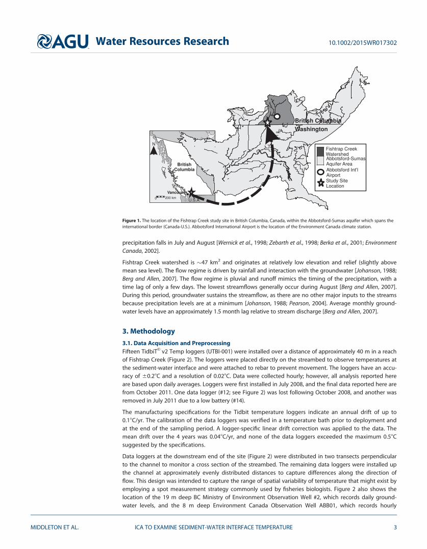
The study site is a reach of Fishtrap Creek, located in the Lower Fraser Valley of southwestern British Colum-bia (BC) (Figure 1). Fishtrap Creek watershed is situated within the regional Abbotsford-Sumas aquifer. Thisparticular reach was selected because it is a gaining reach during the summer [Johanson, 1988; Berg andAllen, 2007]. There is no forest canopy or overhanging vegetation, only seasonal grasses present as in-stream vegetation, so the direct and indirect effects of shading on stream temperature are avoided[Middleton et al., 2015]. The reach is well suited for making comparisons of temperature patterns betweenyears because the channel characteristics, such as summer water depth, bed material, and stream vegeta-tion cover, are stable. This location has other data sources, including a Water Survey of Canada gauging sta-tion at the downstream end of the site (Fishtrap Creek at International Boundary 08MH153), and a climatestation at the nearby Abbotsford International Airport (Climate ID 1100030).

The climate of Fishtrap Creek watershed is Maritime and dominated by moderate temperatures with highannual precipitation rates. The temperatures throughout the year are moderated by the close proximity tothe Pacific Ocean. The annual average precipitation is 1500 mm/yr, with little snow; less than 100 mm aswater. Approximately 70% of precipitation falls in the period between October and May, and only 6% of the

Water Resources Research 10.1002/2015WR017302

MIDDLETON ET AL. ICA TO EXAMINE SEDIMENT-WATER INTERFACE TEMPERATURE 2

precipitation falls in July and August [Wernick et al., 1998; Zebarth et al., 1998; Berka et al., 2001; EnvironmentCanada, 2002].

Fishtrap Creek watershed is �47 km2 and originates at relatively low elevation and relief (slightly abovemean sea level). The flow regime is driven by rainfall and interaction with the groundwater [Johanson, 1988;Berg and Allen, 2007]. The flow regime is pluvial and runoff mimics the timing of the precipitation, with atime lag of only a few days. The lowest streamflows generally occur during August [Berg and Allen, 2007].During this period, groundwater sustains the streamflow, as there are no other major inputs to the streamsbecause precipitation levels are at a minimum [Johanson, 1988; Pearson, 2004]. Average monthly ground-water levels have an approximately 1.5 month lag relative to stream discharge [Berg and Allen, 2007].

3. Methodology

3.1. Data Acquisition and PreprocessingFifteen TidbiTVR v2 Temp loggers (UTBI-001) were installed over a distance of approximately 40 m in a reachof Fishtrap Creek (Figure 2). The loggers were placed directly on the streambed to observe temperatures atthe sediment-water interface and were attached to rebar to prevent movement. The loggers have an accu-racy of 60.28C and a resolution of 0.028C. Data were collected hourly; however, all analysis reported hereare based upon daily averages. Loggers were first installed in July 2008, and the final data reported here arefrom October 2011. One data logger (#12; see Figure 2) was lost following October 2008, and another wasremoved in July 2011 due to a low battery (#14).

The manufacturing specifications for the Tidbit temperature loggers indicate an annual drift of up to0.18C/yr. The calibration of the data loggers was verified in a temperature bath prior to deployment andat the end of the sampling period. A logger-specific linear drift correction was applied to the data. Themean drift over the 4 years was 0.048C/yr, and none of the data loggers exceeded the maximum 0.58Csuggested by the specifications.

Data loggers at the downstream end of the site (Figure 2) were distributed in two transects perpendicularto the channel to monitor a cross section of the streambed. The remaining data loggers were installed upthe channel at approximately evenly distributed distances to capture differences along the direction offlow. This design was intended to capture the range of spatial variability of temperature that might exist byemploying a spot measurement strategy commonly used by fisheries biologists. Figure 2 also shows thelocation of the 19 m deep BC Ministry of Environment Observation Well #2, which records daily ground-water levels, and the 8 m deep Environment Canada Observation Well ABB01, which records hourly

Figure 1. The location of the Fishtrap Creek study site in British Columbia, Canada, within the Abbotsford-Sumas aquifer which spans theinternational border (Canada-U.S.). Abbotsford International Airport is the location of the Environment Canada climate station.

Water Resources Research 10.1002/2015WR017302

MIDDLETON ET AL. ICA TO EXAMINE SEDIMENT-WATER INTERFACE TEMPERATURE 3

groundwater temperatures. Unfortunately, no single observation well recorded both groundwater level andgroundwater temperature over the period of the study.

The multiple time series files from each data logger within each year were joined, time/date formats stand-ardized, and quality assurance/quality control checks on the data performed using Aquarius v. 3.0.75.1[Aquatic Informatics Inc., 2012]. Data gaps up to several hours occurred during downloading events whendata loggers were removed from the stream. These minor gaps were filled using polynomial interpolationwhich was found to provide the best fit for hourly data gaps. The infilling of these gaps has little effect onthe daily temperature series used here.

The analyses were performed in R [R Development Core Team, 2011] using the contributed packages lubri-date [Grolemund and Wickham, 2011] for converting data and time from data loggers, xts [Ryan and Ulrich,2011] for aggregating data to daily time steps, and fastICA [Marchini et al., 2010].

3.2. Heat Balance ModelStream temperature is controlled by fluxes of heat energy that act on the water course, including a combi-nation of radiation, conduction, convection, and advection [Webb, 1996; Webb and Zhang, 1997; Evans et al.,1998; Hannah et al., 2004]. The heat balance in the stream is the combination of energy fluxes at the water-

Figure 2. (a) The distribution of temperature data loggers at the study site. At the data logger locations, a ‘‘/’’ stroke indicates a station lostin 2009 and a ‘‘\’’ lost in 2011. (b) Inset map showing the site location in Fishtrap Creek watershed and the locations of the EnvironmentCanada observation well (ABB01) and the BC observation well (Obs.#2).

Water Resources Research 10.1002/2015WR017302

MIDDLETON ET AL. ICA TO EXAMINE SEDIMENT-WATER INTERFACE TEMPERATURE 4

air interface and the sediment-water interface. Dividing the system into interfaces can be useful for isolatingthe factors influencing the stream temperature which act to add or remove heat from the system [Evanset al., 1998; Hannah et al., 2004]. The daily heat balance was calculated for the water-air interface to isolateclimatic factors that may be influencing how the stream temperature changes as water flows from upstreamto downstream through the reach. We needed to confirm that solar radiation dominated the heat balanceand that other effects (e.g., precipitation events) were negligible.

The simplified heat balance for the site was calculated based on the following equation, following themethods described in Sinokrot and Stefan [1993], Evans et al. [1998], and Xin and Kinouchi [2013] for theexchange of thermal energy across the air-water interface:

Hnet5 Hisð12aÞ2Hl2He2Hc (1)

where Hnet is the net heat exchange at the air-water interface, His is the incident solar radiation, a is thealbedo of the stream surface, Hl is the net longwave radiation, He is the evaporative heat transfer, and Hc isthe convective (sensible) heat transfer. Daily incident solar radiation (His) was estimated using the solar posi-tion and radiation calculator developed by the State of Washington Department of Ecology [2014]. The BirdClear Sky model for direct radiation incident upon a horizontal surface was used, which is based on the lati-tude and elevation of each site [Bird and Hulstrom, 1981]. A value of 0.06 was used for a, following theapproach by Xin and Kinouchi [2013]. The output is a daily estimate of the solar radiation; note that there isno correction for the conditions in the atmosphere except as exhibited in the air temperatures.

The net longwave radiation (Hl) was calculated using the daily mean stream and air temperatures and emis-sivities of the water surface and atmosphere [Xin and Kinouchi, 2013]. The evaporative heat flux (He) was cal-culated using the air temperature, relative humidity, and wind speed from the climate station following Xinand Kinouchi [2013] and Sinokrot and Stefan [1993]. The convective heat flux (Hc) was calculated using theair and mean stream temperatures and the air pressure [Xin and Kinouchi, 2013; Sinokrot and Stefan, 1993].The equations and methods for calculation of the heat budget are presented in more detail in Middletonet al. [2015].

Heat budget plots were examined for variations in the net radiation, and to identify heat budget compo-nents that were dominating those variations. Plotting the daily heat balance for short windows of thesummer period (Figure 3) allowed for comparison of the components that dominate the heat balance underdifferent precipitation conditions as precipitation was not directly considered in the simplified heat budget.Figure 3a shows a 2 week period with precipitation, while Figure 3b shows a period without rainfall. Theabsence of variation in the heat budget components during the wet period indicates that precipitationevents do not appear to impact the daily heat balance for this site. The period with precipitation was exam-ined specifically to evaluate if there were any lags in the daily heat balance as a result of precipitationevents. For both conditions, incoming solar radiation dominates. Net longwave radiation and convectiveheat fluxes remained relatively unchanged in the daily heat balance, and therefore are not considered to beinfluencing factors for individual sediment-water interface temperature measurement locations. However,evaporative fluxes were reflected in the net heat flux for the stream, indicating evaporative processes canbe important to the overall heat balance at a daily time scale. Figure 3 shows that variations in the evapora-tive heat flux are reflected inversely in the net radiation, with no time lag. The strong dependence of theheat balance on solar radiation means that, at this site, the air temperature can be used as a predictor ofthe sediment-water interface temperature to evaluate the influence of solar radiation on the interface tem-peratures. The use of air temperature as a surrogate for solar radiation in the absence of detailed heat fluxdata has been demonstrated in the literature as a reasonable approach [e.g., Smith, 1981; Mohseni and Ste-fan, 1999].

3.3. Estimated Sediment-Water Interface TemperatureBoth air and water temperatures respond to changes in incoming solar radiation; however, water tempera-ture responses are delayed and damped due to the thermal inertia of water. Given that the sediment-waterinterface temperature was expected to correlate with solar radiation to some degree, a daily time series wasneeded for cross-correlation analysis with the ICA extracted components (as discussed later).

Water temperature at the sediment-water interface can be estimated from air temperature through anempirical linear relationship [Stefan and Preud’homme, 1993]. Comparisons between linear relationships and

Water Resources Research 10.1002/2015WR017302

MIDDLETON ET AL. ICA TO EXAMINE SEDIMENT-WATER INTERFACE TEMPERATURE 5

higher-order polynomial relationshipshave found that a linear relationship isappropriate for estimating moderate(08C–208C) water temperatures, whichis the range of Fishtrap Creek summertemperatures [Mohseni et al., 1998;Mohseni and Stefan, 1999; Kelleheret al., 2012]. To relate the air tempera-ture to sediment-water interface tem-perature, it is assumed that the streamis well mixed, uniform, and freeflowing.

The time lag between the air andsediment-water interface temperaturesfor the study site was calculated as30 h. The lag period was found usingthe net surface heat transfer coeffi-cient for heat transfer between theatmosphere and the water surface,and a mean summer water depth atthe study site of 0.78 m [see Middletonet al., 2015]. The value of the heattransfer coefficient of 30 W/m2/8C isconsistent for this stream depth basedon the time lag estimate given inSinokrot and Stefan [1993] for summervalues. For the calculation ofsediment-water interface temperatureat a daily time step, a lag of 1 day wasused for simplicity. Thus, the lag isslightly lower (24 h) compared to thecalculated lag (30 h)—see section 5 for

the implications. The mean daily sediment-water interface temperature was calculated from the mean of allthe interface loggers across the site. Using daily mean air temperatures with only positive values over theperiod of record, the linear relationship between daily sediment-water interface temperature (Ts) and dailyair temperature (Ta), at a lag of 1 day, was determined empirically for the site as:

Ts tð Þ5 5:15 1 0:49 �Taðt21 day�

(2)

where T is in 8C.

3.4. ICAIndependent Component Analysis is a statistically based, signal processing technique that can be usedto separate independent source components from an input of mixed signals that are time series [Comon,1994; Whitfield et al., 1999; Hyvarinen and Oja, 2000; Naik and Kumar, 2011; Hyvarinen, 2012]. The classicexplanation of ICA is the ‘‘cocktail party problem’’; sample data from a number of microphones that‘‘observe’’ people talking simultaneously in a room are separated into individual speech signals. ICA findsthe independent components by maximizing the statistical independence of the estimated components.There are different ways to define independence, and this choice governs the form of the ICA algorithm.The two broadest definitions of independence for ICA are minimization of mutual information and maxi-mization of non-Gaussianity. The non-Gaussianity family of ICA algorithms, which include FastICA, aremotivated by the central limit theory. Typical algorithms for ICA use centering (subtract the mean to cre-ate a zero mean signal), whitening (usually with the eigenvalue decomposition), and dimensionalityreduction. These preprocessing steps are used in order to simplify and reduce the complexity of the

a)

0

5

10

15

20

25

30

35

-100

0

100

200

300

400

500

600

2-May-09

Prec

ipita

tion

(mm

)

Hea

t Tra

nsfe

r (W

/m2 )

0

5

10

15

20

25

30

35

1-Jun-09Pr

ecip

itatio

n (m

m)

Hea

t Tra

nsfe

r (W

/m2 )

Precip Net Radiation Incoming SolarLongwave Evaporative Convective

b)9-May-09 16-May-09

8-Jun-09 15-Jun-09-100

0

100

200

300

400

500

600

Figure 3. Daily heat balance components showing examples from 2009 of earlysummer periods with (a) a period of rainfall and (b) a period without rain.

Water Resources Research 10.1002/2015WR017302

MIDDLETON ET AL. ICA TO EXAMINE SEDIMENT-WATER INTERFACE TEMPERATURE 6

problem for the actual iterative algorithm. Whitening ensures that all dimensions are treated equally apriori before the algorithm is run. ICA cannot identify the actual number of source signals, a uniquelycorrect ordering of the source signals, nor the proper scaling (including sign) of the source signals. ICArequires no prior knowledge of the mixing process and thus is one of the most common forms of blindsignal separation.

The basis of ICA is that recording devices, such as temperature data loggers, record mixed signals (x). Thesemixed signals are products of source signals (s) and some mixing matrix (A), where both s and A areunknown:

x5As (3)

The goal of ICA is to obtain an estimate of the independent source components (s), using the recorded signals(x). The source components (s) can be estimated from the mixed signals (x) and an unmixing matrix (W):

s5Wx (4)

where W 5 A21. The only observed variable is the mixed signal, x, and there is no prior input information onthe original source signals or the mixing matrix, A. This absence of input information is the aspect of themethod that is considered ‘‘blind.’’ To simplify the process, the equations do not consider any noise compo-nents, or time lag in the recordings.

Several ICA algorithms have been discussed in the literature and one of the most common is the FastICAmethod [Hyvarinen, 1997; Hyvarinen and Oja, 1997; Hyvarinen, 1999; Hyvarinen and Oja, 2000; Naik andKumar, 2011]. Fast ICA is a fixed point algorithm that uses higher-order statistics for estimating the inde-pendent source components. The FastICA method [Marchini et al., 2010] performs centering and the pre-whitening, in addition to the ICA component extraction. The ICA separation of mixed signals is based ontwo assumptions and three effects of mixing source signals. The assumptions are (a) the source signals areindependent of each other and (b) the values in each source signal have non-Gaussian distributions. Thethree effects of mixing are:

1. The source signals are independent; however, their signal mixtures are not. This is because the signalmixtures share the same source signals.

2. According to the Central Limit Theorem, the distribution of a sum of independent random variablestends toward a Gaussian distribution. Thus, a sum of two independent random variables usually has adistribution that is closer to Gaussian than any of the two original variables. Here we consider the valueof each signal as the random variable.

3. The temporal complexity of any signal mixture is greater than that of its simplest constituent sourcesignal.

If the components extracted from a set of mixtures are independent (like source signals), or have non-Gaussian histograms (like source signals), or have low complexity (like source signals), then they must besource signals. One can drop the independence assumption and separate mutually correlated signals, thus,statistically ‘‘dependent’’ signals. Whitfield et al. [1999] demonstrated that ICA separation worked well in thepresence of Gaussian noise. Some authors have noted that there is no guarantee that any particular algo-rithm can capture the individual source signals if its components are a nonlinear mixtures [Chawla, 2009]. Insuch cases, ICA does not ensure separation, and emphasizes very large indeterminacies [Jutten et al., 2004].While the transfer of heat into the groundwater is nonlinear, and at some time scales, the temperature ofthe groundwater and the surface water could be correlated, the difference in statistical memory of thesetwo sources suggests that the temperature of the sources can be considered locally independent at a dailytime step. Surface water temperature is linked to air temperature relatively directly, as explained above, andgroundwater temperature is similarly nonlinearly driven at a longer time scale and considerably dampened.The groundwater temperature thus varies only a small amount over a summer. Since the process we areinterested in is the flux of water from different sources, that mixing, and hence the signal mixing, is linearwhich is sufficient to meet our objective of comparing daily signals between years of groundwater heatfluxes. In our study, we take a further step of conducting a cross-correlation analysis with variables that areexpected to be related to the various extracted components, in order to limit ambiguities, and to identifythe main hydrological processes linked to the components.

Water Resources Research 10.1002/2015WR017302

MIDDLETON ET AL. ICA TO EXAMINE SEDIMENT-WATER INTERFACE TEMPERATURE 7

Two ambiguities exist in the ICA output components [Hyvarinen and Oja, 2000; Naik and Kumar, 2011; Hyvar-inen, 2012]. The first is a magnitude and scaling ambiguity, in which the true variance of the independentcomponents cannot be determined. The second is that the order of the estimated sources cannot be deter-mined. Both ambiguities result because the source signals and the mixing matrix are unknown. Thus, norestrictions or conditions are imposed on the sources during separation, leaving the order indistinguishable,and each permutation equally valid.

In this study, ICA was used to perform a blind separation of the component signals contained in the recordsfor each summer for all available temperature loggers. The number of available recorded signals was 15 in2008, 14 in 2009 and 2010, and 13 in 2011. ICA was run for each year using all available loggers as input sig-nals. Any number of components may be extracted; however, as the number of extracted componentsincreases, they become nonunique and it becomes difficult to distinguish between them. The strategy,therefore, was to consider what variables likely contribute to the heat budget of the stream reach, as deter-mined by the simplified heat budget. At this site, solar radiation, stream inflow, and groundwater exchangewere considered the dominant variables. Therefore, three components were extracted.

3.5. Cross-Correlation AnalysisThe extracted temperature components were then compared to three main variables using the cross corre-lation with the ICA components (estimated streambed temperature, stream discharge, and groundwaterlevel). Unsmoothed and smoothed (2 day moving average) stream discharge were considered. Thesmoothed stream discharge was used to strengthen the cross-correlation results by removing the short-term influence of precipitation events on stream discharge. The groundwater temperature remained rela-tively constant over all the summer periods, while the groundwater level fluctuated during and betweenthe summer periods, and for this reason groundwater level is a more appropriate variable to test with crosscorrelation. These variables are considered most likely to relate directly to three contributing variablesdescribed above. Cross correlation provides a value that indicates the strength of the relationship betweenthe variables, and also any lags between the two variables. The sign of the lag indicates which variable leadsin the correlation, with a positive lag indicating that the x variable lags the y, and a negative lag the reverse.The estimated sediment-water interface temperature signal is the x variable in all cross correlations. The lagis useful in evaluating the timing in the interface temperature responses.

4. Results

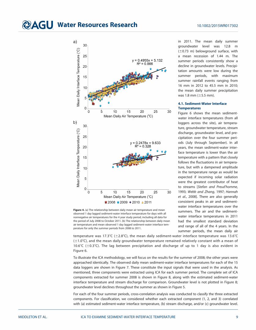
A linear model of daily mean air temperature and the 1 day lagged mean measured sediment-water inter-face temperature for all nonnegative temperatures in the 4 year period was found to explain more than86% of the variance in interface temperature (Figure 4a). In the individual years, the relationship was con-sistent, with the air temperature explaining between 82% and 89% of the variance. The regression slope(0.50) and the positive intercept (5.18C) are characteristic of streams with groundwater contributions, whichmoderate seasonal temperature fluctuations [Smith, 1981; Caissie, 2006]. Over the summer period only, thelinear model explains only 31% of the variance over the four summers (Figure 4b), suggesting that otherfactors dominantly contribute to the remaining variance. In individual summers, the air temperatureexplained between 18% (2011) and 57% (2009) of the variance in the sediment-water interface tempera-ture. In 2008 and 2010, the variance explained was 25% and 23%, respectively. The lower regression slope(0.25) indicates that the interface temperature increases less relative to the increase in air temperature dur-ing summer compared to annually. As this reach is physically uniform, and evaporative fluxes do not domi-nate the heat budget over the summer period, the observed variability in sediment-water interfacetemperatures that are not explained by the estimated sediment-water interface temperature can be attrib-uted to variations in the groundwater flux or other local-scale drivers. The extraction method presentednext seeks to understand these additional components over each summer.

Two important hydrologic variables in this reach of Fishtrap Creek are stream discharge and groundwaterlevel. The mean daily summer stream discharge was 0.20 m3/s (60.25 m3/s), but stream discharge generallydecreased over the summer period, and had peaks associated with precipitation events throughout thesummer. Figure 5a shows mean daily stream discharge over the 2008–2011 period. Groundwater levels inobservation well #2 for the period from 2008 to 2011 are shown in Figure 5b. There is a definite seasonalpattern of groundwater levels and some year to year variation; highest groundwater levels were observed

Water Resources Research 10.1002/2015WR017302

MIDDLETON ET AL. ICA TO EXAMINE SEDIMENT-WATER INTERFACE TEMPERATURE 8

in 2011. The mean daily summergroundwater level was 12.8 m(60.73 m) belowground surface, witha mean recession of 1.44 m. Thesummer periods consistently show adecline in groundwater levels. Precipi-tation amounts were low during thesummer periods, with maximumsummer rainfall events ranging from16 mm in 2012 to 45.5 mm in 2010;the mean daily summer precipitationwas 1.8 mm (65.5 mm).

4.1. Sediment-Water InterfaceTemperaturesFigure 6 shows the mean sediment-water interface temperatures (from allloggers across the site), air tempera-ture, groundwater temperature, streamdischarge, groundwater level, and pre-cipitation over the four summer peri-ods (July through September). In allyears, the mean sediment-water inter-face temperature is lower than the airtemperature with a pattern that closelyfollows the fluctuations in air tempera-ture, but with a dampened amplitudein the temperature range as would beexpected if incoming solar radiationwere the greatest contributor of heatto streams [Stefan and Preud’homme,1993; Webb and Zhang, 1997; Hannahet al., 2008]. There are also generallyconsistent peaks in air and sediment-water interface temperatures over thesummers. The air and the sediment-water interface temperatures in 2011had the smallest standard deviationand range of all of the 4 years. In thesummer periods, the mean daily air

temperature was 17.38C (62.88C), the mean daily sediment-water interface temperature was 13.68C(61.08C), and the mean daily groundwater temperature remained relatively constant with a mean of10.68C (60.38C). The lag between precipitation and discharge of up to 1 day is also evident inFigure 6.

To illustrate the ICA methodology, we will focus on the results for the summer of 2008; the other years wereapproached identically. The observed daily mean sediment-water interface temperatures for each of the 15data loggers are shown in Figure 7. These constitute the input signals that were used in the analysis. Asmentioned, three components were extracted using ICA for each summer period. The complete set of ICAcomponents extracted for summer 2008 is shown in Figure 8, along with the estimated sediment-waterinterface temperature and stream discharge for comparison. Groundwater level is not plotted in Figure 8;groundwater level declines throughout the summer as shown in Figure 5.

For each of the four summer periods, cross-correlation analysis was conducted to classify the three extractedcomponents. For classification, we considered whether each extracted component (1, 2, and 3) correlatedwith (a) estimated sediment-water interface temperature, (b) stream discharge, and/or (c) groundwater level.

Figure 4. (a) The relationship between daily mean air temperature and meanobserved 1 day lagged sediment-water interface temperature for days with allnonnegative air temperatures for the 4 year study period, including all data forthe period of July 2008 to October 2011. (b) The relationship between daily meanair temperature and mean observed 1 day lagged sediment-water interface tem-perature for only the summer periods from 2008 to 2011.

Water Resources Research 10.1002/2015WR017302

MIDDLETON ET AL. ICA TO EXAMINE SEDIMENT-WATER INTERFACE TEMPERATURE 9

Component 1 was most strongly correlated with the estimated sediment-water interface temperature meas-ured over that particular summer. Correlation values were >0.1 (considered significant). The patterns for com-ponents 2 and 3 differed between the summers.

As an example, Figure 9 shows the ICA components for 2008, with the various cross-correlation results. Thetop row is the plot of the time series for each variable, with the cross correlations with each ICA componentsignal shown below. The mean sediment-water interface temperature and the ICA components are shownin the left column, followed by correlations with the estimated 1 day lagged estimated sediment-waterinterface temperature in the second column. The third and fourth columns show the cross correlations withdischarge (unsmoothed discharge, then smoothed with a 2 day moving average). The final column showscross correlation with the groundwater level. For completeness, the cross-correlation results are shown for2009, 2010, and 2011, in supporting information Figures S1–S3.

Because climate conditions varied from summer to summer, there are 12 unique ICA components; 3 in eachof the 4 summer periods. Visual comparison of these components in Figure 9 (for 2008) and the additionalfigures in the supporting information (for 2009–2011), demonstrates the variability between the years (dis-cussed later). Table 1 provides a summary of the results of the cross-correlation tests for each of thesummer periods. Correlations were considered significant when they were both greater than 0.1 andexceeded the calculated statistical significance values on the cross-correlation plot. In Table 1, componentsare listed in order of strongest correlation (e.g., in 2009 groundwater level correlates strongly with compo-nent 2 and to a lesser degree with component 1).

5. Discussion

ICA differs from the analytical approaches that are classically used to examine stream temperatures.Those approaches consider the source signals and relevant noise and bias components (air temperature,

Figure 5. (a) Mean daily stream discharge for Fishtrap Creek and International Boundary for 2008–2011. Data from Water Survey of CanadaStation 08MH153. The summer periods are emphasized by darker symbols. Periods of estimated data are indicated in red. (b) Mean dailygroundwater levels for the period of January 2008 to December 2011. The heavy line sections indicate the summer periods (data from BCMinistry of Environment Observation Well #2).

Water Resources Research 10.1002/2015WR017302

MIDDLETON ET AL. ICA TO EXAMINE SEDIMENT-WATER INTERFACE TEMPERATURE 10

Figure 6. Daily air temperatures, estimated sediment-water interface temperatures, mean daily sediment-water interface temperatures, daily precipitation, stream discharge (all on pri-mary y axis), and groundwater levels (secondary y axis) for the summer periods of 2008–2011. The estimated sediment-water interface temperatures were calculated using equation (2).

Water Resources Research 10.1002/2015WR017302

MIDDLETON ET AL. ICA TO EXAMINE SEDIMENT-WATER INTERFACE TEMPERATURE 11

water temperature, groundwater tem-perature, noise, and sensor drift). Wedo not consider these componentsdirectly. Rather, using ICA, weextracted independent signals fromthe observed time series and corre-lated those signals to variables thatcan influence sediment-water inter-face temperature through inputs tothe heat budget over the distance ofthe stream reach. These variablesinclude the solar radiation, repre-sented by the estimated sediment-water interface temperature; the heatof the incoming streamflow, changesto which are represented by thestream discharge; heat transfer due togroundwater whereby changes in thegroundwater levels reflect the poten-

tial of the groundwater to contribute to the streamflow and thus influence the sediment-water interfacetemperature.

To interpret the ICA and cross-correlation results, Table 2 summarizes the climate and hydrological proc-esses in each summer that are captured across the top row in Figure 9 (supporting information Figures S1–S3). The table ranks each parameter (where [1] is highest and [4] is lowest) and provides generalized com-ments about responses.

The estimated sediment-water interface temperature varied each summer. In all summers except 2010, compo-nent 1 was strongly correlated with estimated interface temperature. This suggests that surface heating from

solar radiation is the dominantfactor influencing the sediment-water interface temperature inmost years. In summer 2008,however, there was a negativelag of 1 day in the correlationbetween the ICA component andthe estimated sediment-waterinterface temperature (Figure 9).The negative lag in the tempera-ture correlation suggests that inthe cool periods, such as in 2008,the 1 day calculated lag for ther-mal energy transfer from solarradiation may be an over estima-tion of the lag. In the othersummer periods, the correlationwith estimated sediment-waterinterface temperature was atzero lag time, indicating that the1 day calculated lag was repre-sentative of the heat transferrate.

Stream discharge differed betweenthe four summers, as might beexpected due to variations in

1-Jul

16-Jul

31-Jul

15-Aug

30-Aug

14-Sep

29-Sep

10

12

14

16

18

)C( erutarep

meTecafretnI ylia

D naeM

o

L15

L5

L8

L2L7

L13L14

L6 L4

L9

L1L3

L11 L10L12

Figure 7. The 15 observed daily mean temperatures at the sediment-water inter-face for 2008. L.1 to L.15 relate to the site locations shown in Figure 2.

Figure 8. The three ICA components (1–3) extracted for summer 2008. The estimatedsediment-water interface temperature and stream discharge are included at the top forcomparison. The units for all ICA components are 8C.

Water Resources Research 10.1002/2015WR017302

MIDDLETON ET AL. ICA TO EXAMINE SEDIMENT-WATER INTERFACE TEMPERATURE 12

precipitation. However, no consistent patterns emerged when comparing the cross-correlation results betweensummers. In contrast, there is a distinct decline in local groundwater levels each summer, although the amount ofdecline varied between the summers. This indicates that groundwater is discharging and contributing to the surfaceflow but that the magnitude of groundwater discharge decreases over the summer and is variable betweensummers. The groundwater may contribute a diffuse influence on the sediment-water interface temperature distrib-uted along the stream channel, or groundwater influxes may be localized, particularly when hyporheic flows are pres-ent due to variations in bed and reach morphology, among other factors. However, because all the loggers werecombined in this study (i.e., ICA was run for all available loggers each year), the diffuse or localized nature of thegroundwater contribution could not be distinguished. A spatial analysis using the ICA method, comparing signalsamong data loggers situated at different locations, may provide greater insight into the spatial variability of ground-water influxes.

In each of the four summer periods, the ICA components correlate to at least one of the three heatcontributing variables (Table 1). In most years, however, more than one component correlated with aparticular heat contributing variable. While independence of the variables is an assumption of ICA,these results suggest that the variables influencing the sediment-water interface temperatures arenot entirely independent. The correlation of the components (Table 1) is related to the trends in thevariables listed in Table 2. In cool wet years, such as 2008, the stream temperatures are lower, whilethe discharge and groundwater levels are higher. In summer 2008, three components correlated tomultiple variables (Table 1), indicating that when variations in groundwater levels are low, the varia-tions in the temperature signals and groundwater contributions are more difficult to separate. In2009, the streamflow and groundwater levels were among the lowest of the summer periods, the airand stream temperatures reached their highest values. In 2009, fewer components were correlated

Figure 9. Results for summer 2008 of the ICA components and the cross correlation with the variables contributing to the heat exchanges. The extracted ICA components are shown inthe left figure (pink) below the mean stream temperature recorded by the data loggers at the sediment-water interface. The cross correlations for each ICA component are shown in red,with the correlated variable shown in the top row of each column. The horizontal dashed lines in the correlation plots mark the 0.1 correlation value, above which the correlations wereconsidered significant.

Water Resources Research 10.1002/2015WR017302

MIDDLETON ET AL. ICA TO EXAMINE SEDIMENT-WATER INTERFACE TEMPERATURE 13

to more than one variable (Table 1).Summer 2010 had moderate rank-ings in all variables, but had thehighest precipitation, whichoccurred mainly in Septemberresulting in the higher streamflows.The mean sediment-water interfacetemperature in 2010 also had thehighest range of values. The compo-nents also correlated with a mix ofvariables in 2010, with only compo-nent 1 correlating with discharge,but all components correlating withestimated sediment-water interfacetemperature and groundwater level.

In 2011, the stream discharge and groundwater levels were high, and the air and stream tempera-tures were low. The lowest range in stream temperature occurred in 2011. One component signal(component 2) in 2011 correlated to both discharge and groundwater levels (Table 1), indicating thatvariation in temperature contributions from these variables are more difficult to separate when theyare both high.

Overall, in all summers, the extracted components were correlated with more than one variable. How-ever, in summers with lower stream discharge and greater stream temperature ranges, the contributingvariables were more easily separated. This inability to completely separate the components and relatethem to specific variables is no doubt a product of the fact that the variables we considered might benonlinear combinations (e.g., the interaction between air temperature and streamflow). Cloudy condi-tions affect air temperature, increase the probability of precipitation, and subsequently discharge andgroundwater level. We suspect that the separations in Table 1 reflect this complex interrelationship.Thus, ICA has limitations in natural settings where, for example, climate influences multiple processesand interactions between processes exist.

Table 1. A Summary of the ICA Components and the Correlations WithPredictor Variablesa

Summer

Estimated Sediment-Water Interface

TemperatureDischarge

(Unsmoothed)

Discharge (2Day Moving

Average)Groundwater

Level

2008 1, 2 2, 3 3, 2 3, 12009 1 3 3 2, 12010 3, 2, 1 1 1 1, 2, 32011 1 2, 1 2, 1 2, 3

aThe table lists the ICA component number (1–3). Each component corre-lates with one or more of the variables listed in the top row. The results for2008 are given in bold for comparison with Figure 9. Correlations were con-sidered significant when they were both greater than 0.1 and exceeded thecalculated statistical significance values on the cross-correlation plot. Compo-nents are listed in order of strongest correlation.

Table 2. Overview of the Climate and Hydrological Observations Over the Four Year Perioda

Summer

Mean/MaxAir Temperature

(8C)

Mean/RangeSediment-Water

InterfaceTemperature

(8C)Total Precipitation

(mm)Median Discharge

(m3/s)

Max/RangeGroundwater

Level/(m)

2008 16.8 [4]/23.6 [3] 13.8 [3]/5.2 [2] 186 [2] Most in August 0.11 [2] Discharge punctuatedwith several moderately highdischarge events from lateJuly to mid-August thatpersisted for several days

13.6 [3]/1.0 [4]Declined throughoutthe summer

2009 18.1 [1]/28.8 [1] 14.6 [4]/8.1 [1] 155 [4] 0.05 [4] In late-July, there was ahigh discharge period whichlasted approximately 4 dayswith maximum mean dailyflow up to 1.0 m3/s

14.0 [1]/1.4[3]Declined throughoutthe summer

2010 17.3 [2]/25.9 [2] 14.1 [2]/4.7 [3] 252 [1] Most in September 0.1 [3] Rain events correspondedto the periods of high dischargefrom mid-August to September

13.6 [2]/1.4 [2]Declined fromJuly to August withlittle variation inSeptember

2011 17.3 [3]/22.1[4] [1] 13.3 [4]/3.6 [4] 182 [3] Rainfall eventswere mainly in earlyJuly and late September

0.2 [1] Very few high dischargeevents from mid-Julyto mid-September.Discharge remained highthroughout the summer periodrelative to the previous summers

12.8 [4]/1.9 [1]Declined throughoutthe summer

aRank is shown in ‘‘[]’’ with [1] the highest and [4] the lowest.

Water Resources Research 10.1002/2015WR017302

MIDDLETON ET AL. ICA TO EXAMINE SEDIMENT-WATER INTERFACE TEMPERATURE 14

Nevertheless, some broad observations can be made based on the ICA results, which enhance our under-standing of the system. Specifically, thermal exchanges appear to be taking place in addition to the air-water interface. These exchanges also take place at the sediment-water interface, and the correlation withgroundwater levels indicates these heat exchanges are associated with groundwater inflow. The results arenot surprising given that Fishtrap Creek has been described as a groundwater-fed stream [Berg and Allen,2007]. This study provides stronger evidence that in some years (e.g., 2009) the sediment-water interfacetemperature is highly influenced by groundwater inflows across the site. Based on the spatial variability ofthe component signals (results not shown), the locations of groundwater inflow are variably distributedacross this site, indicating that this reach is influenced by a combination of focused and diffuse ground-water discharge.

Other studies have similarly reported temporal variability of groundwater inflows [e.g., Constantz,1998; Wroblicky et al., 1998; Keery et al., 2007]. The inflow of groundwater to streams was reported inthese studies to be a complex process, with scale-dependent variability occurring both spatially andtemporally. Temporally, variability can range from diurnal to interannual as shown in this study. Herewe have demonstrated the use of ICA in blind separation of mixed signals from temperature loggers atthe sediment-water interface and assessed how those component signals can be used to identifyimportant heat transfer processes. While there were some ambiguities in the extracted signals, likelydue to nonindependence of the temperature signal components, the use of cross correlation helped toreduce these ambiguities. Without cross correlation, it was challenging to associate a particularextracted component with a particular variable, with the exception of the estimated sediment-waterinterface temperature, which was both visually similar to component 1 and often had a high correla-tion with it in most years.

The value of ICA is that temperature signals from multiple data loggers can be evaluated against known, orsuspected, variables. A priori knowledge of these variables (here estimated sediment-water interface tem-perature, stream discharge, and groundwater level) helped to determine the number of components forextraction. In previous iterations of this work, we used ICA somewhat blindly, and extracted several compo-nents. Through experimentation, we ultimately settled on three to reflect the dominant processes at thesite. Other studies may benefit from this approach, but a reasonable conceptual model of the site is war-ranted in order to focus the analysis.

Finally, as mentioned above, other applications of ICA in the hydrological sciences should beexplored. In particular, given the presence of multidimensional flows such as those due to hyporheicflows, and the high degree of spatial heterogeneity in streambed and aquifer hydraulic propertiesthat may influence the temperatures (and fluxes), a spatial analysis using ICA may prove particularlyuseful at some sites.

6. Conclusions

The study focused on the summer period of July to September, when streamflow in the studied coastalstream is low and the relative contribution of groundwater to streamflow is often the highest for the year.Sediment-water interface temperatures in this small 40 m reach of Fishtrap Creek are controlled by multipleprocesses. The dominant process is the transfer of thermal energy from the atmosphere to the stream andthen to the streambed in each of the four summers. Stream discharge and groundwater contributions influ-ence the observed sediment-water interface temperatures and their importance varied between the foursummers reported here. The contributions of these processes are complex, varying between and within thesummer periods. It is demonstrated that components of observed sediment-water interface temperaturesextracted using ICA can be used to interpret information from multiple sediment-water interface tempera-ture sensors.

The timing and magnitude of discharge in the summer periods as well as annual groundwater levels areimportant factors in the distribution of the temperature components across the stream reach. Separa-tion of the temperature components is more apparent during summers with lower flows, and greaterstream temperature ranges. While solar radiation is the dominant thermal contribution to the reach,observed sediment-water interface temperatures are modified by streamflow variations and ground-water inputs.

Water Resources Research 10.1002/2015WR017302

MIDDLETON ET AL. ICA TO EXAMINE SEDIMENT-WATER INTERFACE TEMPERATURE 15

ReferencesAires, F., A. Chedin, and J. Nadal (2000), Independent component analysis of multivariate time series: Application to the tropical SST vari-

ability, J. Geophys. Res., 103, 17,437–17,455, doi:10.1029/2000JD900152.Alexander, M., and D. Caissie (2003), Variability and comparison of hyporheic water temperatures and seepage fluxes in a small Atlantic

Salmon stream, Ground Water, 41(1), 72–82.Anderson, M. (2005), Heat as a ground water tracer, Ground Water, 43(6), 951–968, doi:10.1111/j.1745-6584.2005.00052.x.Aquatic Informatics Inc. (2012), Aquarius Time Series Software (v. 3.0.75.1), Vancouver, B. C., Canada.Benyahya, L., D. Caissie, A. St-Hilaire, T. Ouarda, and B. Bobee (2007), A review of statistical water temperature models, Can. Water Resour.

J., 32(2), 179–192.Berg, M. A., and D. M. Allen (2007), Low flow variability in groundwater-fed streams, Can. Water Resour. J., 32(3), 227–245, doi:10.4296/cwrj3203227.Berka, C., H. Scheier, and K. Hall (2001), Linking water quality with agricultural intensification in a rural watershed, Water Air Soil Pollut., 127,

389–401.Bird, R. E., and R. L. Hulstrom (1981), Simplified clear sky model for direct and diffuse insolation on horizontal surfaces, Tech. Rep. SERI/TR

642-761, Sol. Energy Res. Inst., Golden, Colo.Bogan, T., O. Mohseni, and H. G. Stefan (2003), Stream temperature-equilibrium temperature relationship, Water Resour. Res., 39(9), 1245,

doi:10.1029/2003WR002034.Brewer, S. K. (2013), Groundwater influences on the distribution and abundance of riverine smallmouth bass, Micropterus dolomieu, in pas-

ture landscapes of the Midwestern USA, River Res. Appl., 29, 269–278.Briggs, M. A., E. B. Voytek, F. D. Day-Lewis, D. O. Rosenberry, and J. W. Lane (2013), Understanding water column and streambed thermal

refugia for endangered mussels in the Delaware River, Environ. Sci. Technol., 47(20), 11,423–11,431.Brunke, M., and T. Gonser (1997), The ecological significance of exchange processes between rivers and groundwater, Freshwater Biol., 37,

1–33, doi:10.1046/j.1365-2427.1997.00143.x.Caissie, D. (1991), The importance of groundwater to fish habitat: Base flow characteristics for three Gulf Region rivers, Can. Data Rep. Fish.

Aquat. Sci. 814, 25 pp., Department of Fisheries and Oceans, Science Branch, Moncton, New Brunswick, Canada.Caissie, D. (2006), The thermal regime of rivers: A review, Freshwater Biol., 51(8), 1389–1406, doi:10.1111/j.1365-2427.2006.01597.x.Caissie, D., B. L. Kurylyk, A. St-Hilaire, N. El-Jabi, and K. T. B. MacQuarrie (2014), Streambed temperature dynamics and corresponding heat

fluxes in small streams experiencing seasonal ice cover, J. Hydrol., 519, 1441–1452.Chawla, M. P. S. (2009), Detection of indeterminacies in corrected ECG signals using parameterized multidimensional independent compo-

nent analysis, Comput. Math. Methods Med., 10(2), 85–115.Comon, P. (1994), Independent component analysis: A new concept?, Signal Processes, 36, 287–314, doi:10.1016/0165-1684(94)90029-9.Conant, B. (2004), Delineating and quantifying ground water discharge zones using interface temperatures, Ground Water, 42(2), 243–257,

doi:10.1111/j.1745-6584.2004.tb02671.x.Constantz, J. (2008), Heat as a tracer to determine streambed water exchanges, Water Resour. Res., 44, W00D10, doi:10.1029/2008WR006996.Constantz, J. (1998), Interaction between stream temperature, streamflow, and groundwater exchanges in alpine streams, Water Resour. Res.,

34(7), 1609–1615.Cunjak, R. A., T. Linnansaari, and D. Caissie (2013), The complex interaction of ecology and hydrology in a small catchment: A salmon’s per-

spective, Hydrol. Processes, 27, 741–749.Environment Canada (2002), Canadian Cslimate Normals Online, CDCD West CD, 2009 [online], Vancouver, B. C. [Available at http://climate.

weatheroffice.ec.gc.ca.proxy.lib.sfu.ca/prods_servs/cdcd_iso_e.html.]Evans, E. C., and G. E. Petts (1997), Hyporheic temperature patterns within riffles, Hydrol. Sci., 42(2), 199–213, doi:10.1080/02626669709492020.Evans, E. C., G. R. McGregor, and G. E. Petts (1998), River energy budgets with special reference to river bed processes, Hydrol. Processes, 12,

575–595, doi:10.1002/(SICI)1099-1085(19980330)12:4< 575::AID-HYP595> 3.0.CO;2-Y.Fleming, S. W., P. H. Whitfield, R. D. Moore, and E. J. Quilty (2007), Regime-dependent streamflow sensitivities to Pacific climate modes

cross the Georgia-Puget transboundary ecoregion, Hydrol. Processes, 21, 3264–3287.Funaro, M., E. Oja, and H. Valpola (2003), Independent component analysis for artefact separation in astrophysical images, Neural Networks,

16(3–4), 469–478, doi:10.1016/S0893-6080(03)00017-0.Grolemund, G., and H. Wickham (2011), Dates and times made easy with lubridate, J. Stat. Software, 40, 1–25.Hannah, D. M., I. A. Malcolm, C. Soulsby, and A. F. Youngson (2004), Heat exchanges and temperatures within a salmon spawning stream

in the Cairngorms, Scotland: Seasonal and sub-seasonal dynamics, River Res. Appl., 20, 635–652, doi:10.1002/rra.771.Hannah, D. M., I. A. Malcolm, C. Soulsby, and A. F. Youngson (2008), A comparison of forest and moorland stream microclimate, heat

exchanges and thermal dynamics, Hydrol. Processes, 22, 919–940, doi:10.1002/hyp.7003.Hatch, C. E., A. T. Fisher, J. S. Revenaugh, J. Constantz, and C. Ruehl (2006), Quantifying surface water–groundwater interactions using time

series analysis of streambed thermal records: Method development, Water Resour. Res., 42, W10410, doi:10.1029/2005WR004787.Hyvarinen, A. (1997), A family of fixed-point algorithms for independent component analysis, IEEE Int. Conf. Acoust. Speech Signal Process, 5,

3917–3920, doi:10.1109/ICASSP.1997.604766.Hyvarinen, A. (1999), Fast and robust fixed-point algorithms of independent component analysis, IEEE Neural Networks, 10(3), 626–634, doi:

10.1109/72.761722.Hyvarinen, A. (2012), Independent component analysis: Recent advances, Philos. Trans. R. Soc. A, 371, 1–20, doi:10.1098/rsta.2011.0534.Hyvarinen, A., and E. Oja (1997), A fast fixed-point algorithm for independent component analysis, Neural Comput., 9(7), 1483–1492, doi:

10.1162/neco.1997.9.7.1483.Hyvarinen, A., and E. Oja (2000), Independent component analysis: Algorithms and applications, Neural Networks, 13(4–5), 411–430,

doi:10.1016/S0893-6080(00)00026-5.Irvine, D. J., R. H. Cranswick, C. T. Simmons, M. A. Shanafield, and L. K. Lautz (2015), The effect of streambed heterogeneity on groundwater-

surface water exchange fluxes inferred from temperature time series, Water Resour. Res., 51, 198–212, doi:10.1002/2014WR015769.Johanson, D. (1988), Fishtrap/Pepin/Bertrand Creeks Watershed Management Basin Plan: Groundwater Component, Prov. of B. C. Minist. of

Environ. and Parks, Water Manage. Branch, Surrey, B. C., Canada.Johnson, S. L., and J. A. Jones (2000), Stream temperature responses to forest harvest and debris flows in western Cascades, Oregon, Can.

J. Fish Aquat. Sci., 57, 30–39, doi:10.1139/f00-109.Jutten, C., M. Babaie-Zadeh, and S. Hosseini (2004), Three easy ways for separating nonlinear mixtures?, Signal Process., 84, 217–229.Keery, J., A. Binley, N. Crook, and J. Smith (2007), Temporal and spatial variability of groundwater-surface water fluxes: Development and

application of an analytical method using temperature time series, J. Hydrol., 336(1–2), 1–16, doi:10.1016/j.jhydrol.2006.12.003.

AcknowledgmentsThis research was supported by theNatural Sciences and EngineeringResearch Council (NSERC) through aDiscovery Grant to Diana Allen, as wellas research grants from Simon FraserUniversity’s Community TrustEndowment Fund (CTEF), WatershedWatch Salmon Society, and the PacificInstitute for Climate Solutions. Theanalyses were performed in R [RDevelopmsent Core Team, 2011] usingthe contributed packages; the authorsand the maintainers of these packagesare gratefully acknowledged. Theauthors would like to thank theanonymous reviewers for theirvaluable comments. The data used inthis manuscript can be requested fromthe corresponding author.

Water Resources Research 10.1002/2015WR017302

MIDDLETON ET AL. ICA TO EXAMINE SEDIMENT-WATER INTERFACE TEMPERATURE 16

Kelleher, C., T. Wagener, M. Gooseff, B. McGlynn, K. McGuire, and L. Marshall (2012), Investigating controls on the thermal sensitivity ofPennsylvania streams, Hydrol. Processes, 26, 771–785.

Krause, S., T. Blume, and N. J. Cassidy (2012), Investigating patterns and controls of groundwater up-welling in a lowland river by combin-ing fibre-optic distributed temperature sensing with observations of vertical hydraulic gradients, Hydrol. Earth Syst. Sci., 16, 1775–1792,doi:10.5194/hess-16-1775-2012.

Kurylyk, B. L., K. T. B. MacQuarrie, and C. I. Voss (2014), Climate change impacts on the temperature and magnitude of groundwater dis-charge from shallow, unconfined aquifers, Water Resour. Res., 50, 3253–3274, doi:10.1002/2013WR014588.

Marchini, J. L., C. Heaton, and B. D. Ripley (2010), fastICA: FastICA Algorithms to Perform ICA and Projection Pursuit. R Package Version 1.1-13[online]. [Available at http://CRAN.R-project.org/package5fastICA.]

Mayer, T. D. (2012), Controls of summer stream temperature in the Pacific Northwest, J. Hydrol., 475, 323–335.Middleton, M. A., D. M. Allen, and P. H. Whitfield (2015), Comparing the groundwater contribution in two groundwater-fed streams using a

combination of methods, Can. Water Resour. J., doi:10.1080/07011784.2015.1068136, in press.Mitiandoudis, N., and M. E. Davies (2003), Audio source separation of convolutive mixtures, IEEE Trans. Speech Audio Process., 5, 489–497,

doi:10.1109/TSA.2003.815820.Mohseni, O., and H. G. Stefan (1999), Stream temperature/air temperature relationship: A physical interpretation, J. Hydrol., 218, 128–141.Mohseni, O., H. G. Stefan, and T. R. Erickson (1998), A nonlinear regression model for weekly stream temperatures, Water Resour. Res., 34, 2685–2692.Moore, R. D., D. L. Spittlehouse, and A. Story (2005), Riparian microclimate and stream temperature response to forest harvest: A review, J.

Am. Water Resour. Assoc., 41(4), 813–834, doi:10.1111/j.1752-1688.2005.tb03772.x.Moore, R. D., M. Nelitz, and E. Parkinson (2013), Empirical modelling of maximum weekly average stream temperature in British Columbia,

Canada, to support assessment of fish habitat suitability, Can.Water Resour. J., 38, 135–147.Moradkhani, H., and M. Meier (2010), Long-lead water supply forecast using large-scale climate predictors and independent component

analysis, J. Hydrol. Eng., 15(10), 744–762, doi:10.1061/(ASCE)HE.1943-5584.0000246.Naik, G. R., and D. K. Kumar (2011), An overview of independent component analysis and its applications, Informatica, 35, 63–81.Pearson, M. P. (2004), The ecology, status and recovery prospects of Nooksack Dace (Rhinichthys cataractae spp.) and Salish Sucker (Catos-

tomus sp.) in Canada, PhD thesis, 239 pp., Univ. of B. C., Vancouver, B. C., Canada.Poole, G., and C. H. Berman (2001), An ecological perspective on in-stream temperature: Natural heat dynamics and mechanisms of

human-caused thermal degradation, Environ. Manage., 27(6), 787–802, doi:10.1007/s002670010188.Power, G., R. S. Brown, and J. G. Imhof (1999), Groundwater and fish—Insights from northern North America, Hydrol. Processes, 13(3), 401–

422, doi:10.1002/(SICI)1099-1085(19990228)13:3< 401::AID-HYP746> 3.0.CO;2-A.R Development Core Team (2011), R: A Language and Environment for Statistical Computer, R Found. for Stat. Comput., Vienna. [Available at

http://www.R-project.org/.]Rau, G. C., M. S. Andersen, A. M. McCallum, and R. I. Acworth (2010), Analytical methods that use natural heat as a tracer to quantify surface

water-groundwater exchange, evaluated using field temperature records, Hydrogeol. J., 18(5), 1093–1110.Rau, G. C., M. S. Andersen, A. M. McCallum, H. Roshan, and R. I. Acworth (2014), Heat as a tracer to quantify water flow in near-surface sedi-

ments, Earth Sci. Rev., 129, 40–58.Ryan, J., and J. M. Ulrich (2011), xts: Extensible Time Series. R Package Version 0.8.2 [online]. [Available at http://CRAN.R-project.org/packages5xts.]Silliman, S. E., and D. F. Booth (1993), Analysis of time-series measurements of sediment temperature for identification of gaining vs. losing

portions of Juday Creek, Indiana, J. Hydrol., 146(1–4), 131–148, doi:10.1016/0022-1694(93)90273-C.Sinokrot, B. A., and H. G. Stefan (1993), Stream temperature dynamics: Measurements and modeling, Water Resour. Res., 29, 2299–2312,

doi:10.1016/0022-1694(93)90273-C.Smakhtin, V. (2001), Low flow hydrology: A review, J. Hydrol., 240(3–4), 147–186, doi:10.1016/S0022-1694(00)00340-1.Smith, K. (1981), The prediction of river water temperature, Hydrol. Sci. Bull., 26(1), 19–32, doi:10.1080/02626668109490859.Sophocleous, M. (2007), The science and practice of environmental flows and the role of hydrogeologists, Ground Water, 45(4), 393–401,

doi:10.1111/j.1745-6584.2007.00322.x.State of Washington Department of Ecology (2014), Solrad.v. 1.2: A Solar Position and Radiation Calculator for Microsoft Excel/VBA [online].

[Available at http://www.ecy.wa.gov/programs/eap/models.html.]Stefan, H. G., and E. B. Preud’homme (1993), Stream temperature estimation from air temperature, Water Resour. Bull., 29(1), 27–45, doi:

10.1111/j.1752-1688.1993.tb01502.x.Ungureanu, M., C. Bigan, R. Strungaru, and V. Lazarescu (2004), Independent component analysis applied in biomedical signal processing,

Meas. Sci. Rev., 4, 8.Velasco-Cruz, C., S. C. Lehman, M. Hudy, and E. P. Smith (2012), Assessing the risk of rising temperature on brook trout: A spatial dynamic

linear risk model, J. Agric. Biol. Environ. Stat., 17(2), 246–264.Webb, B. W. (1996), Trends in stream and river temperature, Hydrol. Processes, 10, 205–226, doi:10.1002/(SICI)1099-1085(199602)10:

2< 205::AID-HYP358> 3.0.CO;2-1.Webb, B. W., and Y. Zhang (1997), Spatial and seasonal variability in the components of the river heat budget, Hydrol. Processes, 11, 79–

101, doi:10.1002/(SICI)1099-1085(199701)11:1< 79::AID-HYP404> 3.0.CO;2-N.Wernick, B. G., K. E. Cook, and H. Schreier (1998), Land use and streamwater nitrate-N dynamics in an urban-rural fringe watershed, J. Am.

Water Resour. Assoc., 34, 639–650, doi:10.1111/j.1752-1688.1998.tb00961.x.Westra, S., C. Brown, L. Umanu, and A. Sharma (2007), Modeling multivariate hydrological series: Principal component analysis or inde-

pendent component analysis?, Water Resour. Res., 43, W06429, doi:10.1029/2006WR005617.Whitfield, P. H., M. J. R. Clark, and A. Cannon (1999), Signals and noise in environmental data—Characterization of non-random uncertainty in

environmental monitoring, in Environmental Modeling. Proceedings of the International Conference on Water, Environment, Ecology, Socio-Economics and Health Engineering (WEESHE), edited by V. P. Singh, W. I. Seo, and J. H. Sonu, pp. 86–95, Water Resour. Publ. LLC, HighlandsRanch, Colo.

Winter, T. C., J. W. Harvey, O. L. Franke, and W. M. Alley (1998), Groundwater and surface water—A single resource, U.S. Geol. Surv. Circ., 1139, 1–17.Wroblicky, G. J., M. E. Campana, H. M. Valett, and C. N. Dahn (1998), Seasonal variation in surface-subsurface water exchange and lateral

hyporheic area of two stream-aquifer systems, Water Resour. Res., 34, 317–328, doi:10.1029/97WR03285.Xin, Z., and T. Kinouchi (2013), Analysis of stream temperature and heat budget in an urban river under strong anthropogenic influences, J.

Hydrol., 489, 16–25, doi:10.1016/j.jhydrol.2013.02.048.Zebarth, B. J., B. Hii, H. Liebcher, K. Chipperfield, J. W. Paul, G. Grove, and S. Y. Szeto (1998), Agricultural land use practices and nitrate con-

tamination in the Abbotsford Aquifer, British Columbia, Canada, Agric. Ecosyst. Environ., 69, 99–112, doi:10.1016/S0167-8809(98)00100-5.

Water Resources Research 10.1002/2015WR017302

MIDDLETON ET AL. ICA TO EXAMINE SEDIMENT-WATER INTERFACE TEMPERATURE 17