Embed Size (px)
Citation preview
INDEPENDENT COMPONENT ANALYSIS (ICA) APPLIED TO LONG
BUNCH BEAMS IN THE LOS ALAMOS PROTON STORAGE RING∗
J. Kolski† , R. Macek, R. McCrady, X. Pang, LANL, Los Alamos, NM, 87545, USA
Abstract
Independent component analysis (ICA) is a powerful
blind source separation (BSS) method[1]. Compared to the
typical BSS method, principal component analysis (PCA),
which is the BSS foundation of the well known model in-
dependent analysis (MIA)[2], ICA is more robust to noise,
coupling, and nonlinearity[3, 4, 5]. ICA of turn-by-turn
beam position data has been used to measure the trans-
verse betatron phase and amplitude functions, dispersion
function, linear coupling, sextupole strength, and nonlinear
beam dynamics[3, 4, 5]. We apply ICA in a new way to
slices along the bunch, discuss the source signals identified
as betatron motion and longitudinal beam structure, and for
betatron motion, compare the results of ICA and PCA.
INTRODUCTION
We apply BSS in a new way to slices along the bunch[6].
We digitize beam signals from the Los Alamos Proton
Storage Ring (PSR) for a full injection-extraction cycle,
≥ 1800 turns. We divide the digitized signal into time
slices of equal length using the 0.5 ns digitization bin
length. The long digitized signal vector is stacked turn-
by-turn to form the data matrix
x(t) =
x1(1) x1(2) . . . x1(N)x2(1) x2(2) . . . x2(N)
......
. . ....
xM (1) xM (2) . . . xM (N)
, (1)
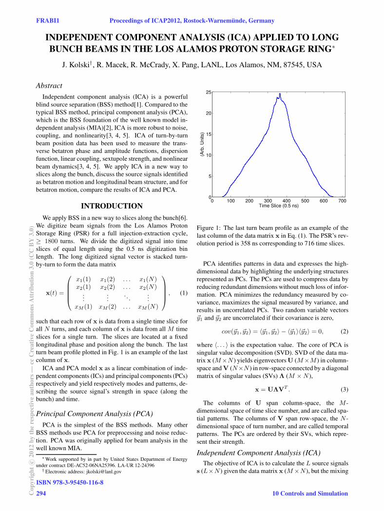
such that each row of x is data from a single time slice for
all N turns, and each column of x is data from all M time
slices for a single turn. The slices are located at a fixed
longitudinal phase and position along the bunch. The last
turn beam profile plotted in Fig. 1 is an example of the last
column of x.
ICA and PCA model x as a linear combination of inde-
pendent components (ICs) and principal components (PCs)
respectively and yield respectively modes and patterns, de-
scribing the source signal’s strength in space (along the
bunch) and time.
Principal Component Analysis (PCA)
PCA is the simplest of the BSS methods. Many other
BSS methods use PCA for preprocessing and noise reduc-
tion. PCA was originally applied for beam analysis in the
well known MIA.
∗Work supported by in part by United States Department of Energy
under contract DE-AC52-06NA25396. LA-UR 12-24396† Electronic address: [email protected]
0 100 200 300 400 500 600 7000
5
10
15
20
25
Time Slice (0.5 ns)(A
rb. U
nits)
Figure 1: The last turn beam profile as an example of the
last column of the data matrix x in Eq. (1). The PSR’s rev-
olution period is 358 ns corresponding to 716 time slices.
PCA identifies patterns in data and expresses the high-
dimensional data by highlighting the underlying structures
represented as PCs. The PCs are used to compress data by
reducing redundant dimensions without much loss of infor-
mation. PCA minimizes the redundancy measured by co-
variance, maximizes the signal measured by variance, and
results in uncorrelated PCs. Two random variable vectors
~y1 and ~y2 are uncorrelated if their covariance is zero,
cov(~y1, ~y2) = 〈~y1, ~y2〉 − 〈~y1〉〈~y2〉 = 0, (2)
where 〈. . . 〉 is the expectation value. The core of PCA is
singular value decomposition (SVD). SVD of the data ma-
trix x (M×N ) yields eigenvectorsU (M×M ) in column-
space and V (N×N ) in row-space connected by a diagonal
matrix of singular values (SVs) Λ (M ×N ),
x = UΛVT . (3)
The columns of U span column-space, the M -
dimensional space of time slice number, and are called spa-
tial patterns. The columns of V span row-space, the N -
dimensional space of turn number, and are called temporal
patterns. The PCs are ordered by their SVs, which repre-
sent their strength.
Independent Component Analysis (ICA)
The objective of ICA is to calculate the L source signals
s (L×N ) given the data matrix x (M×N ), but the mixing
FRABI1 Proceedings of ICAP2012, Rostock-Warnemünde, Germany
ISBN 978-3-95450-116-8
294Cop
yrig
htc ○
2012
byth
ere
spec
tive
auth
ors—
ccC
reat
ive
Com
mon
sAtt
ribu
tion
3.0
(CC
BY
3.0)
10 Controls and Simulation
matrix A (M × L) is unknown
x = As. (4)
ICA assumes independent source signals, a stricter re-
quirement than PCA. Two random variable vectors ~y1 and
~y2 are independent if the covariance of any function of ~y1and any function of ~y2 is zero,
〈f(~y1), g(~y2)〉 − 〈f(~y1)〉〈g(~y2)〉 = 0. (5)
For time series data, source signal independence is re-
lated to diagonality of covariance matrices[7]. The auto-
covariance of a signal is cov(~yi(t), ~yi(t− τ)), where τ is a
time lag, τ = 0, 1, 2, . . . Similarly, the covariance between
two signals is cov(~yi(t), ~yj(t − τ)) where i 6= j. Apply-
ing these two results to mean-zero signals for reasons to
become evident later, we write the time-lagged covariance
matrix
Cy(τ) = 〈y(t)y(t − τ)T 〉. (6)
Source signal independence requires the time-lagged co-
variance matrices Cs(τ) = 〈s(t)s(t− τ)T 〉 be diagonal,
〈si(t)sj(t− τ)T 〉 = 0, i 6= j, τ = 0, 1, 2, . . . . (7)
It follows that A−1x must also possess diagonal time-
lagged covariance matrices. The BSS problem is solved
by obtaining a demixing matrix that diagonalizes the time-
lagged covariance matrices of x.
The zero time-lagged covariance matrix Cx(τ = 0)does not contain enough information to obtain the mix-
ing matrix A. The key is to utilize the additional infor-
mation contained in the time-lagged covariance matrices
Cx(τ). Including more than one time lag improves ICA’s
performance by resolving degenerate SVs, but it introduces
an additional complication of simultaneously diagonaliz-
ing many Cx(τ). A numerical technique for simultane-
ously diagonalizing several matrices with Jacobi angles is
discussed in Ref. [8]. Typically, 20 - 50 time lags are re-
quired to separate source signals with close SVs[4, 5]. We
use the ICA algorithm Second Order Blind Identification
(SOBI)[7], which accommodates multiple time lags, in our
analysis and outline the algorithm below:
1. Whitening
The data matrix x is preprocessed to obtain mean-zero,
whitened (yyT = I) data. Mean-zero data, which sim-
plifies the covariance matrix calculation, is calculated by
subtracting the average over the temporal variation. SVD
is applied to the zero time-lagged covariance matrix of the
mean-zero data matrix x
Cx(0) = 〈x(t)x(t)T 〉
=(
U1,U2
)
(
Λ1 00 Λ2
)(
UT1
UT2
)
,(8)
where Λ1 and Λ2 are diagonal matrices of SVs separated
by a cutoff threshold λc such that min(diag[Λ1]) ≥ λc ≥
max(diag[Λ2]). The cutoff threshold λc is determined by
the number of SVs L included in the analysis. U1 and U2
are eigenvectors corresponding to Λ1 and Λ2 respectively.
The mean-zero, whitened data is calculated
z = Yx, (9)
where zzT = I , Y = Λ−1/21
UT1
, and Λ−1/21
indicates the
inverse square root of the diagonal elements individually.
2. Joint diagonalization
The time-lagged covariance matrices of the mean-zero,
whitened data matrix z are calculated for a set of time lags
(τk, k = 0, 1, . . . , K)
Cz(τk) = 〈z(t)z(t − τk)T 〉. (10)
Modified time-lagged covariance matrices Cz(τk) are con-
structed from Cz(τk)
Cz(τk) =(
Cz(τk) +Cz(τk)T)
/2. (11)
SVD is well defined, since Cz(τk) is real and symmetric
Cz(τk) = WDkWT , (12)
where W is the unitary demixing matrix and Dk is a diag-
onal matrix. The Jacobi angle technique discussed in Ref.
[8] is used to find the demixing matrix W, which is a joint
diagonalizer for all Cz(τk). The mixing matrix A and the
source signals s are calculated
A = Y−1W and s = WTYx. (13)
The columns of A span column-space, the M -
dimensional space of time slice number, and are called
spatial modes. The rows of s span row-space, the N -
dimensional space of turn number, and are called temporal
modes.
INDEPENDENT COMPONENTS
We digitize beam signals from a short stripline beam po-
sition monitor (BPM) with 400 MHz peak frequency re-
sponse. We digitize the BPM’s vertical sum and difference
signals for BSS.
We typically ran our SOBI analysis for L = 30 SVs,
K = 50 time lags, and as many turns as possible.
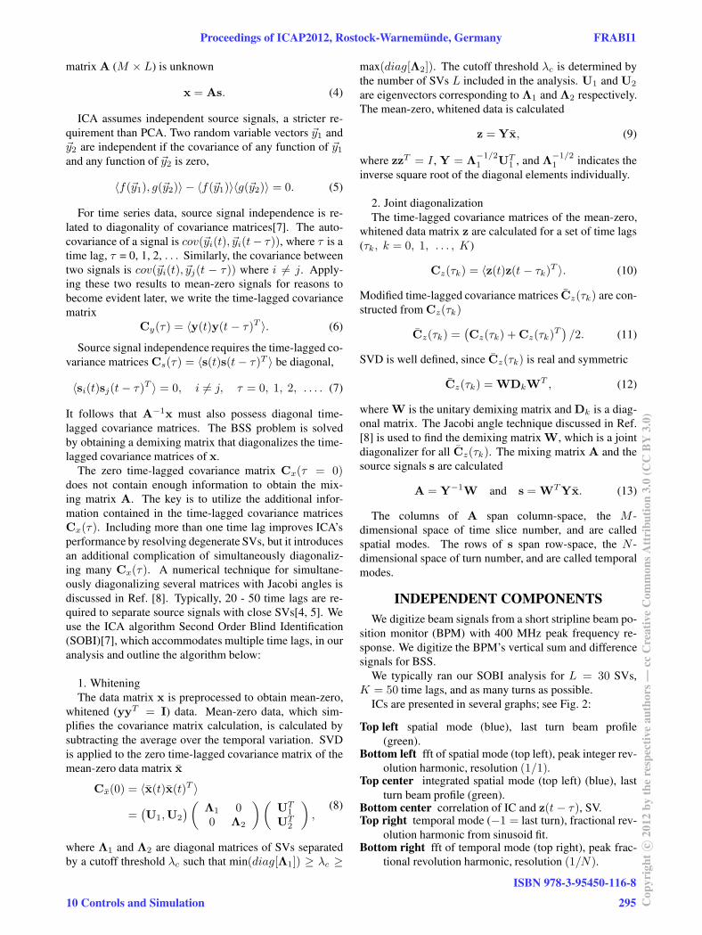
ICs are presented in several graphs; see Fig. 2:
Top left spatial mode (blue), last turn beam profile
(green).Bottom left fft of spatial mode (top left), peak integer rev-
olution harmonic, resolution (1/1).Top center integrated spatial mode (top left) (blue), last
turn beam profile (green).Bottom center correlation of IC and z(t − τ), SV.Top right temporal mode (−1 = last turn), fractional rev-
olution harmonic from sinusoid fit.Bottom right fft of temporal mode (top right), peak frac-
tional revolution harmonic, resolution (1/N).
Proceedings of ICAP2012, Rostock-Warnemünde, Germany FRABI1
10 Controls and Simulation
ISBN 978-3-95450-116-8
295 Cop
yrig
htc ○
2012
byth
ere
spec
tive
auth
ors—
ccC
reat
ive
Com
mon
sAtt
ribu
tion
3.0
(CC
BY
3.0)
0 200 400 600−3
−2
−1
0
1
2
3
Time Slice
A2 (
Arb
. U
nits)
wm41vd f 10/9/2006
0 100 200 3000
20
40
60
80
100
120
Integer Revolution Harmonic
|Y(t
)|
Max 12
0 200 400 600−30
−20
−10
0
10
20
30
Time Slicecum
sum
(A2)
(Arb
. U
nits)
0 20 40−1.0
−0.5
0.0
0.5
1.0
Time Lag
Corr
ela
tion
SV = 50.48
−3000 −2000 −1000 0−0.10
−0.05
0.00
0.05
0.10
Turn
s2 (
Arb
. U
nits)
Fit 0.1804
0 0.2 0.40
2
4
6
8
Fractional Revolution Harmonic
|Y(t
)| ×
10
−3
Max 0.1805
Betatron ICs
In previous applications, ICA obtains quality ICs repre-
senting betatron motion [3, 4, 5], so the betatron IC result
from slices along the bunch is of interest. We induce coher-
ent betatron oscillation with a single-turn kick. The beam
is stored for 420 turns (150 µs) after the kick.
The IC in Fig. 2 is identified as betatron motion because
the fractional revolution harmonic (bottom right) is close
to the operating fractional betatron tune value 0.1805 and
because the temporal mode (top right) is only nonzero for
turns after the single-turn kick.
The spatial mode (top left) indicates the strength of the
0.1805 fractional betatron tune oscillation along the beam
bunch. However, in this case it is easier to interpret the inte-
grated spatial mode (top center) because it has units propor-
tional to current, whereas the spatial mode has units propor-
tional to the derivative of the current. The integrated spatial
mode maximums indicate that the majority of particles un-
dergoing coherent betatron motion with a fractional tune
of 0.1805 are located symmetric about the bunch center at
time slices 237 and 474 and represent the coherent space
charge tune shifted beam. The fast oscillation slightly for-
ward of the bunch center describes mixing of betatron tunes
for the central time slices.
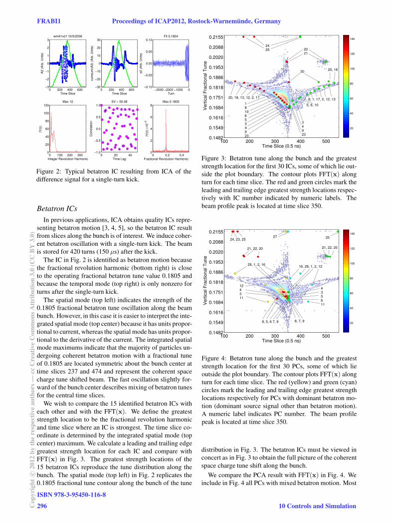
We wish to compare the 15 identified betatron ICs with
each other and with the FFT(x). We define the greatest
strength location to be the fractional revolution harmonic
and time slice where an IC is strongest. The time slice co-
ordinate is determined by the integrated spatial mode (top
center) maximum. We calculate a leading and trailing edge
greatest strength location for each IC and compare with
FFT(x) in Fig. 3. The greatest strength locations of the
15 betatron ICs reproduce the tune distribution along the
bunch. The spatial mode (top left) in Fig. 2 replicates the
0.1805 fractional tune contour along the bunch of the tune
100 200 300 400 5000.1482
0.1549
0.1616
0.1684
0.1751
0.1818
0.1886
0.1953
0.2020
0.2088
0.2155
Time Slice (0.5 ns)
Ve
rtic
al F
ractio
na
l T
un
e
20
40
60
80
100
120
140
20, 18, 13, 12, 2, 17
2425 22
21
30
5, 6, 10
20, 18
8, 1, 17, 2, 12, 13
18106534923
34923
100 200 300 400 5000.1482
0.1549
0.1616
0.1684
0.1751
0.1818
0.1886
0.1953
0.2020
0.2088
0.2155
Time Slice (0.5 ns)
Ve
rtic
al F
ractio
na
l T
un
e
20
40
60
80
100
120
140
21, 22, 20
27 2524, 23, 25
8, 7, 9
21, 22, 20
435611
124311
29, 1, 2, 1616, 29, 1, 2, 12
8, 5, 6 7, 9
distribution in Fig. 3. The betatron ICs must be viewed in
concert as in Fig. 3 to obtain the full picture of the coherent
space charge tune shift along the bunch.
We compare the PCA result with FFT(x) in Fig. 4. We
include in Fig. 4 all PCs with mixed betatron motion. Most
Figure 3: Betatron tune along the bunch and the greateststrength location for the first 30 ICs, some of which lie out-side the plot boundary. The contour plots FFT(x) alongturn for each time slice. The red and green circles mark theleading and trailing edge greatest strength locations respec-tively with IC number indicated by numeric labels. Thebeam profile peak is located at time slice 350.
Figure 2: Typical betatron IC resulting from ICA of thedifference signal for a single-turn kick.
Figure 4: Betatron tune along the bunch and the greateststrength location for the first 30 PCs, some of which lieoutside the plot boundary. The contour plots FFT(x) alongturn for each time slice. The red (yellow) and green (cyan)circles mark the leading and trailing edge greatest strengthlocations respectively for PCs with dominant betatron mo-tion (dominant source signal other than betatron motion).A numeric label indicates PC number. The beam profilepeak is located at time slice 350.
FRABI1 Proceedings of ICAP2012, Rostock-Warnemünde, Germany
ISBN 978-3-95450-116-8
296Cop
yrig
htc ○
2012
byth
ere
spec
tive
auth
ors—
ccC
reat
ive
Com
mon
sAtt
ribu
tion
3.0
(CC
BY
3.0)
10 Controls and Simulation
betatron PCs have peak strengths located near the bunch
center where the difference signal is largest because PCA
is unable to diagonalize the frequency continuum beyond
its peak strength and average location. It is clear from Fig.
4 that PCA is unable to recover the coherent space charge
tune shift along the bunch.
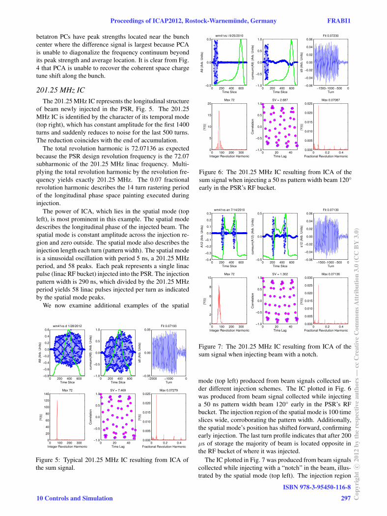
201.25 MHz IC
The 201.25 MHz IC represents the longitudinal structure
of beam newly injected in the PSR, Fig. 5. The 201.25
MHz IC is identified by the character of its temporal mode
(top right), which has constant amplitude for the first 1400
turns and suddenly reduces to noise for the last 500 turns.
The reduction coincides with the end of accumulation.
The total revolution harmonic is 72.07136 as expected
because the PSR design revolution frequency is the 72.07
subharmonic of the 201.25 MHz linac frequency. Multi-
plying the total revolution harmonic by the revolution fre-
quency yields exactly 201.25 MHz. The 0.07 fractional
revolution harmonic describes the 14 turn rastering period
of the longitudinal phase space painting executed during
injection.
The power of ICA, which lies in the spatial mode (top
left), is most prominent in this example. The spatial mode
describes the longitudinal phase of the injected beam. The
spatial mode is constant amplitude across the injection re-
gion and zero outside. The spatial mode also describes the
injection length each turn (pattern width). The spatial mode
is a sinusoidal oscillation with period 5 ns, a 201.25 MHz
period, and 58 peaks. Each peak represents a single linac
pulse (linac RF bucket) injected into the PSR. The injection
pattern width is 290 ns, which divided by the 201.25 MHz
period yields 58 linac pulses injected per turn as indicated
by the spatial mode peaks.
We now examine additional examples of the spatial
0 200 400 600−0.8
−0.6
−0.4
−0.2
0.0
0.2
0.4
0.6
Time Slice
A8
(A
rb.
Un
its)
wm41vs d 1/28/2012
0 100 200 3000
20
40
60
80
100
120
140
Integer Revolution Harmonic
|Y(t
)|
Max 72
0 200 400 600−1.0
−0.5
0.0
0.5
1.0
Time Slice
cu
msu
m(A
8)
(Arb
. U
nits)
0 20 40−1.0
−0.5
0.0
0.5
1.0
Time Lag
Co
rre
latio
n
SV = 7.469
−2000 −1000 0−0.05
0.00
0.05
Turn
s8
(A
rb.
Un
its)
Fit 0.07193
0 0.2 0.40.000
0.005
0.010
0.015
0.020
0.025
Fractional Revolution Harmonic
|Y(t
)|
Max 0.07279
0 200 400 600−0.5
0.0
0.5
Time Slice
A9
(A
rb.
Un
its)
wm41vs i 9/25/2010
0 100 200 3000
5
10
15
20
Integer Revolution Harmonic
|Y(t
)|
Max 72
0 200 400 600−1.0
−0.5
0.0
0.5
1.0
Time Slice
cu
msu
m(A
9)
(Arb
. U
nits)
0 20 40−1.0
−0.5
0.0
0.5
1.0
Time Lag
Co
rre
latio
n
SV = 2.687
−1500−1000 −500 0−0.06
−0.04
−0.02
0.00
0.02
0.04
0.06
Turn
s9
(A
rb.
Un
its)
Fit 0.07230
0 0.2 0.40.000
0.005
0.010
0.015
0.020
0.025
Fractional Revolution Harmonic
|Y(t
)|
Max 0.07087
0 200 400 600−0.4
−0.3
−0.2
−0.1
0.0
0.1
0.2
0.3
Time Slice
A1
2 (
Arb
. U
nits)
wm41vs an 7/14/2010
0 100 200 3000
2
4
6
8
10
Integer Revolution Harmonic
|Y(t
)|
Max 72
0 200 400 600−0.5
0.0
0.5
Time Slice
cu
msu
m(A
12
) (A
rb.
Un
its)
0 20 40−1.0
−0.5
0.0
0.5
1.0
Time Lag
Co
rre
latio
n
SV = 1.302
−1500−1000 −500 0−0.06
−0.04
−0.02
0.00
0.02
0.04
0.06
Turn
s1
2 (
Arb
. U
nits)
Fit 0.07130
0 0.2 0.40.000
0.005
0.010
0.015
0.020
0.025
0.030
Fractional Revolution Harmonic
|Y(t
)|
Max 0.07136
mode (top left) produced from beam signals collected un-
der different injection schemes. The IC plotted in Fig. 6
was produced from beam signal collected while injecting
a 50 ns pattern width beam 120◦ early in the PSR’s RF
bucket. The injection region of the spatial mode is 100 time
slices wide, corroborating the pattern width. Additionally,
the spatial mode’s position has shifted forward, confirming
early injection. The last turn profile indicates that after 200
µs of storage the majority of beam is located opposite in
the RF bucket of where it was injected.
The IC plotted in Fig. 7 was produced from beam signals
collected while injecting with a “notch” in the beam, illus-
trated by the spatial mode (top left). The injection region
Figure 6: The 201.25 MHz IC resulting from ICA of thesum signal when injecting a 50 ns pattern width beam 120◦
early in the PSR’s RF bucket.
Figure 7: The 201.25 MHz IC resulting from ICA of thesum signal when injecting beam with a notch.
Figure 5: Typical 201.25 MHz IC resulting from ICA ofthe sum signal.
Proceedings of ICAP2012, Rostock-Warnemünde, Germany FRABI1
10 Controls and Simulation
ISBN 978-3-95450-116-8
297 Cop
yrig
htc ○
2012
byth
ere
spec
tive
auth
ors—
ccC
reat
ive
Com
mon
sAtt
ribu
tion
3.0
(CC
BY
3.0)
0 200 400 600−0.8
−0.6
−0.4
−0.2
0.0
0.2
0.4
0.6
Time Slice
A2
(A
rb.
Un
its)
wm41vs e 7/14/2010
0 100 200 3000
20
40
60
80
100
Integer Revolution Harmonic
|Y(t
)|
Max 72
0 200 400 600−1.0
−0.5
0.0
0.5
1.0
Time Slicecu
msu
m(A
2)
(Arb
. U
nits)
0 20 40−1.0
−0.5
0.0
0.5
1.0
Time Lag
Co
rre
latio
n
SV = 5.668
−2000 −1000 0−0.05
0.00
0.05
Turn
s2
(A
rb.
Un
its)
Fit 0.009947
0 0.2 0.40.000
0.005
0.010
0.015
0.020
0.025
Fractional Revolution Harmonic
|Y(t
)|
Max 0.009775
widths are 60 time slices, and the notch width between the
two injection regions is 180 time slices. The spatial mode
reproduces the notch injection scheme: inject for 30 ns, no
injection for 90 ns (notch), and inject for 30 ns.
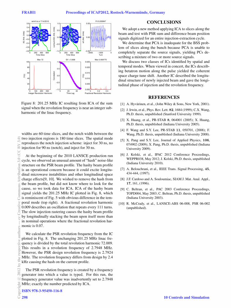
At the beginning of the 2010 LANSCE production run
cycle, we observed an unusual amount of “hash” noise-like
structure on the PSR beam profile. The hashy beam profile
is an operational concern because it could excite longitu-
dinal microwave instabilities and other longitudinal space
charge effects[9, 10]. We wished to remove the hash from
the beam profile, but did not know where to look for the
cause, so we took data for ICA. ICA of the hashy beam
signal yields the 201.25 MHz IC plotted in Fig. 8, which
is reminiscent of Fig. 5 with obvious difference in the tem-
poral mode (top right). A fractional revolution harmonic
0.009 describes an oscillation that repeats every 111 turns.
The slow injection rastering causes the hashy beam profile
by longitudinally stacking the beam upon itself more than
in nominal operations where the fractional revolution har-
monic is 0.07.
We calculate the PSR revolution frequency from the IC
plotted in Fig. 8. The unchanging 201.25 MHz linac fre-
quency is divided by the total revolution harmonic 72.009.
This results in a revolution frequency of 2.7948 MHz.
However, the PSR design revolution frequency is 2.7924
MHz. The revolution frequency differs from design by 2.4
kHz causing the hash on the current profile.
The PSR revolution frequency is created by a frequency
generator into which a value is typed. For this run, the
frequency generator value was inadvertently set to 2.7948
MHz; exactly the number predicted by ICA.
CONCLUSIONS
We adopt a new method applying ICA to slices along the
beam and test with PSR sum and difference beam position
signals digitized for an entire injection-extraction cycle.
We determine that PCA is inadequate for the BSS prob-
lem of slices along the bunch because PCA is unable to
completely separate the source signals, yielding PCs de-
scribing a mixture of two or more source signals.
We discuss two classes of ICs identified by spatial and
temporal modes. When viewed in concert, the ICs describ-
ing betatron motion along the pulse yielded the coherent
space charge tune shift. Another IC described the longitu-
dinal structure of newly injected beam and gave the longi-
tudinal phase of injection and the revolution frequency.
REFERENCES
[1] A. Hyvarinen, et al., (John Wiley & Sons, New York, 2001).
[2] J. Irwin, et al., Phys. Rev. Lett. 82, 1684 (1999); C.X. Wang,Ph.D. thesis, unpublished (Stanford University 1999).
[3] X. Huang, et al., PR-STAB 8, 064001 (2005); X. Huang,Ph.D. thesis, unpublished (Indiana University 2005).
[4] F. Wang and S.Y. Lee, PR-STAB 11, 050701, (2008); F.Wang, Ph.D. thesis, unpublished (Indiana University 2008).
[5] X. Pang and S.Y. Lee, Journal of Applied Physics, 106,074902 (2009); X. Pang, Ph.D. thesis, unpublished (IndianaUniversity 2009).
[6] J. Kolski, et al., IPAC 2012 Conference Proceedings,WEPPR038, May 2012; J. Kolski, Ph.D. thesis, unpublished(Indiana University 2010).
[7] A. Belouchrani, et al., IEEE Trans. Signal Processing, 45,434-444, (1997).
[8] J.F. Cardoso and A. Souloumiac, SIAM J. Mat. Anal. Appl.,17, 161, (1996).
[9] C. Beltran, et al., PAC 2003 Conference Proceedings,TOPD004, May 2003; C. Beltran, Ph.D. thesis, unpublished(Indiana University 2003).
[10] R. McCrady, et al., LANSCE-ABS 06-008, PSR 06-002(unpublished).
Figure 8: 201.25 MHz IC resulting from ICA of the sumsignal when the revolution frequency is near an integer sub-harmonic of the linac frequency.
FRABI1 Proceedings of ICAP2012, Rostock-Warnemünde, Germany
ISBN 978-3-95450-116-8
298Cop
yrig
htc ○
2012
byth
ere
spec
tive
auth
ors—
ccC
reat
ive
Com
mon
sAtt
ribu
tion
3.0
(CC
BY
3.0)
10 Controls and Simulation