Embed Size (px)
Citation preview
Faster independent component analysis by
preconditioning with Hessian approximations
Pierre Ablin ∗, Jean-Francois Cardoso †, and Alexandre Gramfort ‡
September 11, 2017
Abstract
Independent Component Analysis (ICA) is a technique for unsuper-vised exploration of multi-channel data that is widely used in observa-tional sciences. In its classic form, ICA relies on modeling the data aslinear mixtures of non-Gaussian independent sources. The maximizationof the corresponding likelihood is a challenging problem if it has to be com-pleted quickly and accurately on large sets of real data. We introduce thePreconditioned ICA for Real Data (Picard) algorithm, which is a relativeL-BFGS algorithm preconditioned with sparse Hessian approximations.Extensive numerical comparisons to several algorithms of the same classdemonstrate the superior performance of the proposed technique, espe-cially on real data, for which the ICA model does not necessarily hold.
Keywords : Independent Component Analysis, Blind source separation,quasi-Newton methods, maximum likelihood estimation, second order methods,preconditioning.
1 Introduction
Independent Component Analysis (ICA) [1, 2] is a multivariate data explorationtool massively used across scientific disciplines such as neuroscience [3, 4, 5, 6],astronomy [7, 8, 9], chemistry [10, 11] or biology [12, 13]. The underlyingassumption of ICA is that the data are obtained by combining latent componentswhich are statistically independent. The linear ICA problem addresses the casewhere latent variables and observations are linked by a linear transform. Then,ICA boils down to estimating a linear transform of the input signals into ‘sourcesignals’ which are as independent as possible.
∗P. Ablin works at Inria, Parietal Team, Universite Paris-Saclay, Saclay, France; e-mail:[email protected]†J. F. Cardoso is with the Institut d’Astrophysique de Paris, CNRS, Paris, France; e-mail:
[email protected]‡A. Gramfort is with Inria, Parietal Team, Universite Paris-Saclay, Saclay, France; e-mail:
1
arX
iv:1
706.
0817
1v3
[st
at.M
L]
8 S
ep 2
017
The strength and wide applicability of ICA come from its limited number ofassumptions. For ICA to become a well-posed problem it is only required thatall sources except one are non-Gaussian and statistically independent [1]. Thegenerality of this concept explains the usefulness of ICA in many domains.
An early and popular ICA algorithm is Infomax [14]. It is widely usedin neuroscience and is distributed in most neural processing toolboxes (e.g.EEGLAB [15] or MNE [16]). It can be shown to be a maximum likelihoodestimator [17] based on a non Gaussian component model. However, Infomaxmaximizes the likelihood using a stochastic gradient algorithm which may re-quire some hand-tuning and often fails to converge [18], or only converges slowly.
Since speed is important in data exploration, various methods have beenproposed for a faster maximization of the Infomax likelihood by using curvatureinformation, that is by exploiting not only the gradient of the likelihood as inInfomax but also its second derivatives. We briefly review some of the methodsfound in the literature.
The most natural way of using curvature is to use the complete set of secondderivatives (the Hessian) to set up the Newton method but it faces several dif-ficulties: the Hessian is a large object, costly to evaluate and to invert for largedata sets. It also has to be regularized since the ICA likelihood is not convex.The cost issue is addressed in [19] by using a truncated Newton algorithm: anapproximate Newton direction is found by an early stopping (truncation) of itscomputation via a conjugate gradient method. Further, each step in this com-putation is quickly computed by a ‘Hessian-free’ formula. Another approach toexploit curvature is to use approximations of the Hessian, obtained by assum-ing that the current signals are independent (see e.g. [20, 21] or section 2). Forinstance, a simple quasi-Newton method is proposed in [22] and in AMICA [23],and a trust-region algorithm in [24].
We have re-implemented and compared these methods (see section 5) andfound that the Hessian approximations do yield a low cost per iteration butthat they are not accurate enough on real data (which cannot be expected tofollow the ICA model at high accuracy, e.g. in presence of some correlatedsources). The approach investigated in this article overcomes this problem byusing an optimization algorithm which ‘learns’ curvature from the past iterationsof the solver (L-BFGS [25]), and accelerates it by preconditioning with Hessianapproximations.
This article is organized as follows. In section 2, we recall the expressionof the gradient and Hessian of the log-likelihood. We show how simple Hes-sian approximations can be obtained and regularized. That allows the L-BFGSmethod to be preconditioned at low cost yielding the Preconditioned ICA forReal Data (Picard) algorithm described in section 3. In section 4, we detail re-lated algorithms mentioned in the introduction. Finally, section 5 illustrates thesuperior behavior of the Picard algorithm by extensive numerical experimentson synthetic signals, on multiple electroencephalography (EEG) datasets, onfunctional Magnetic Resonance Imaging (fMRI) data and on natural images.
2
2 Likelihood and derivatives
Notation
The Frobenius matrix scalar product is denoted by 〈M |M ′〉 = Tr(M>M ′) =∑i,j MijM
′ij , and ‖M‖ =
√〈M |M〉 is the associated Frobenius matrix norm.
Let B be a fourth order tensor of size N×N×N×N . Its application to a N×NmatrixM is denotedBM , aN×N matrix with entries (BM)ij =
∑k,lBijklMkl.
We also denote 〈M ′|B|M〉 = 〈M ′|BM〉 =∑
i,j,k,lBijklM′ijMkl. The Kronecker
symbol δij equals 1 for i = j and 0 otherwise.The complexity of an operation is said to go as Θ(f(N,T )) for a real function
f if there exist two constants 0 < c1 < c2 such that the cost of that operationis in the interval [c1f(N,T ), c2f(N,T )] for all T,N .
2.1 Non Gaussian likelihood for ICA
The ICA likelihood for a data set X = [x1, .., xN ]> ∈ RN×T of N signalsx1, . . . , xN of length T is based on the linear model X = AS where the N ×N mixing matrix A is unknown and the source matrix S has N statisticallyindependent zero-mean rows. If each row of S is modeled as i.i.d. with pi(·)denoting the common distribution of the samples of the ith source, the likelihoodof A is then [20]:
p(X|A) =
T∏t=1
1
|det(A)|
N∏i=1
pi([A−1x]i(t)) . (1)
It is convenient to work with the negative averaged log-likelihood parametrizedby the unmixing matrix W = A−1, that is, L(W ) = − 1
T log p(X|W−1). It isgiven by:
L(W ) = − log|det(W )| − E
[N∑i=1
log(pi(yi(t))
], (2)
where E denotes the empirical mean (sample average) and where, implicitly,Y = WX. Our aim is to minimize L(W ) with respect to W which amounts tosolving the ICA problem in the maximum likelihood sense.
We note from the start that this optimization problem is not convex for asimple reason: if W ∗ minimizes the objective function, any permutation of thecolumns of W ∗ gives another equivalent minimizer.
In this paper, we focus on fast and accurate minimization of L(W ) for agiven source model, that is, working with fixed predetermined densities pi. Itcorresponds to the standard Infomax model commonly used in practice. Inparticular, our experiments use − log(pi(·)) = 2 log(cosh(·/2)) + cst, which isthe density model in standard Infomax.
In the following, the ICA mixture model is said to hold if the signals actuallyare a mixture of independent components. We stress that on real data, the ICAmixture model is not expected to hold exactly.
3
2.2 Relative variations of the objective function
The variation of L(W ) with respect to a relative variation of W is described, upto second order, by the Taylor expansion of L((I + E)W ) in terms of a ‘small’N ×N matrix E :
L((I + E)W ) = L(W ) + 〈G|E〉+1
2〈E|H|E〉+O(||E||3). (3)
The first order term is controlled by the N × N matrix G, called the relativegradient [26] and the second-order term depends on the N ×N ×N ×N tensorH, called the relative Hessian [22]. Both these quantities can be obtained fromthe second order expansions of log det(·) and log pi(·):
log|det(I + E)| = Tr(E)− 1
2Tr(E2) +O(||E||3),
log(pi(y + e)) = log(pi(y))− ψi(y)e− 1
2ψ′i(y)e2 +O(e3),
where ψi = −p′i
piis called the score function (equal to tanh(·/2) for the standard
Infomax density). Collecting and re-arranging terms yields at first-order theclassic expression
Gij = E[ψi(yi)yj ]− δij or G(Y ) =1
Tψ(Y )Y > − Id (4)
and, at second order, the relative Hessian:
Hijkl = δilδjk + δik E[ψ′i(yi)yjyl] . (5)
Note that the relative Hessian is sparse. Indeed, it has only of the order ofN3 non-zero coefficients: δilδjk 6= 0 for i = l and j = k which corresponds toN2 coefficients, and δik 6= 0 for i = k which happens N3 times. This means thatfor a practical application with 100 sources the Hessian easily fits in memory.However, its computation requires the evaluation of the terms E[ψ′i(yi)yjyl],resulting in a Θ(N3×T ) complexity. This fact and the necessity of regularizingthe Hessian (which is not necessarily positive definite) in Newton methods mo-tivate the consideration of Hessian approximations which are faster to computeand easier to regularize.
2.3 Hessian Approximations
The Hessian approximations are discussed on the basis of the following moments:hijl = E[ψ′i(yi)yjyl] , for 1 ≤ i, j, l ≤ N
hij = E[ψ′i(yi)y2j ] , for 1 ≤ i, j ≤ N
hi = E[ψ′i(yi)] , for 1 ≤ i ≤ Nσ2i = E[y2i ] , for 1 ≤ i ≤ N
. (6)
4
Hence, the true relative Hessian is Hijkl = δilδjk+δikhijl. A first approximation
of H consists in replacing hijl by δjlhij . We denote that approximation by H2:
H2ijkl = δilδjk + δikδjlhij . (7)
A second approximation, denoted H1, goes one step further and replaces hij by
hiσ2j for i 6= j: {
H1ijkl = δilδjk + δikδjlhiσ
2j , for i 6= j
H1iiii = 1 + hii
. (8)
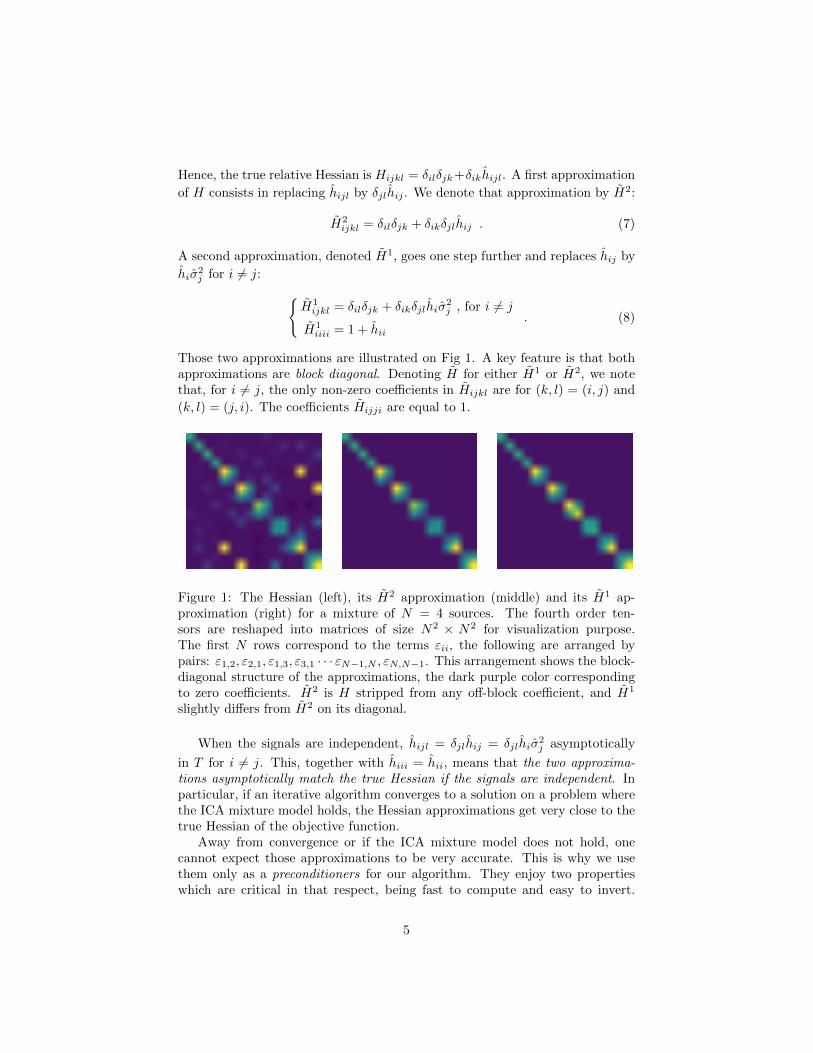
Those two approximations are illustrated on Fig 1. A key feature is that bothapproximations are block diagonal. Denoting H for either H1 or H2, we notethat, for i 6= j, the only non-zero coefficients in Hijkl are for (k, l) = (i, j) and
(k, l) = (j, i). The coefficients Hijji are equal to 1.
Figure 1: The Hessian (left), its H2 approximation (middle) and its H1 ap-proximation (right) for a mixture of N = 4 sources. The fourth order ten-sors are reshaped into matrices of size N2 × N2 for visualization purpose.The first N rows correspond to the terms εii, the following are arranged bypairs: ε1,2, ε2,1, ε1,3, ε3,1 · · · εN−1,N , εN,N−1. This arrangement shows the block-diagonal structure of the approximations, the dark purple color correspondingto zero coefficients. H2 is H stripped from any off-block coefficient, and H1
slightly differs from H2 on its diagonal.
When the signals are independent, hijl = δjlhij = δjlhiσ2j asymptotically
in T for i 6= j. This, together with hiii = hii, means that the two approxima-tions asymptotically match the true Hessian if the signals are independent. Inparticular, if an iterative algorithm converges to a solution on a problem wherethe ICA mixture model holds, the Hessian approximations get very close to thetrue Hessian of the objective function.
Away from convergence or if the ICA mixture model does not hold, onecannot expect those approximations to be very accurate. This is why we usethem only as a preconditioners for our algorithm. They enjoy two propertieswhich are critical in that respect, being fast to compute and easy to invert.
5
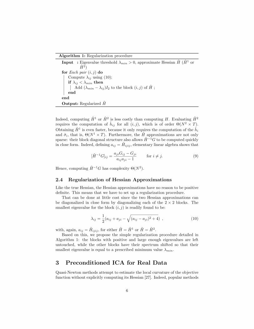
Algorithm 1: Regularization procedure
Input : Eigenvalue threshold λmin > 0, approximate Hessian H (H1 orH2)
for Each pair (i, j) doCompute λij using (10);if λij < λmin then
Add (λmin − λij)I2 to the block (i, j) of H ;end
end
Output: Regularized H
Indeed, computing H1 or H2 is less costly than computing H. Evaluating H2
requires the computation of hij for all (i, j), which is of order Θ(N2 × T ).
Obtaining H1 is even faster, because it only requires the computation of the hiand σi, that is, Θ(N1 × T ). Furthermore, the H approximations are not onlysparse: their block diagonal structure also allows H−1G to be computed quicklyin close form. Indeed, defining aij = Hijij , elementary linear algebra shows that
[H−1G]ij =ajiGij −Gji
aijaji − 1for i 6= j. (9)
Hence, computing H−1G has complexity Θ(N2).
2.4 Regularization of Hessian Approximations
Like the true Hessian, the Hessian approximations have no reason to be positivedefinite. This means that we have to set up a regularization procedure.
That can be done at little cost since the two Hessian approximations canbe diagonalized in close form by diagonalizing each of the 2 × 2 blocks. Thesmallest eigenvalue for the block (i, j) is readily found to be:
λij =1
2(aij + aji −
√(aij − aji)2 + 4) , (10)
with, again, aij = Hijij , for either H = H1 or H = H2.Based on this, we propose the simple regularization procedure detailed in
Algorithm 1: the blocks with positive and large enough eigenvalues are leftuntouched, while the other blocks have their spectrum shifted so that theirsmallest eigenvalue is equal to a prescribed minimum value λmin.
3 Preconditioned ICA for Real Data
Quasi-Newton methods attempt to estimate the local curvature of the objectivefunction without explicitly computing its Hessian [27]. Indeed, popular methods
6
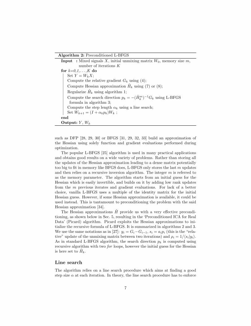
Algorithm 2: Preconditioned L-BFGS
Input : Mixed signals X, initial unmixing matrix W0, memory size m,number of iterations K
for k=0,1,. . . ,K doSet Y = WkX;Compute the relative gradient Gk using (4);
Compute Hessian approximation Hk using (7) or (8);
Regularize Hk using algorithm 1;
Compute the search direction pk = −(Hmk )−1Gk using L-BFGS
formula in algorithm 3;Compute the step length αk using a line search;Set Wk+1 = (I + αkpk)Wk ;
endOutput: Y , Wk
such as DFP [28, 29, 30] or BFGS [31, 29, 32, 33] build an approximation ofthe Hessian using solely function and gradient evaluations performed duringoptimization.
The popular L-BFGS [25] algorithm is used in many practical applicationsand obtains good results on a wide variety of problems. Rather than storing allthe updates of the Hessian approximation leading to a dense matrix potentiallytoo big to fit in memory like BFGS does, L-BFGS only stores the last m updatesand then relies on a recursive inversion algorithm. The integer m is referred toas the memory parameter. The algorithm starts from an initial guess for theHessian which is easily invertible, and builds on it by adding low rank updatesfrom the m previous iterates and gradient evaluations. For lack of a betterchoice, vanilla L-BFGS uses a multiple of the identity matrix for the initialHessian guess. However, if some Hessian approximation is available, it could beused instead. This is tantamount to preconditioning the problem with the saidHessian approximation [34].
The Hessian approximations H provide us with a very effective precondi-tioning, as shown below in Sec. 5, resulting in the ‘Preconditioned ICA for RealData’ (Picard) algorithm. Picard exploits the Hessian approximations to ini-tialize the recursive formula of L-BFGS. It is summarized in algorithms 2 and 3.We use the same notations as in [27]: yi = Gi−Gi−1, si = aipi (this is the “rela-tive” update of the unmixing matrix between two iterations) and ρi = 1/〈si|yi〉.As in standard L-BFGS algorithm, the search direction pk is computed usingrecursive algorithm with two for loops, however the initial guess for the Hessianis here set to Hk.
Line search
The algorithm relies on a line search procedure which aims at finding a goodstep size α at each iteration. In theory, the line search procedure has to enforce
7
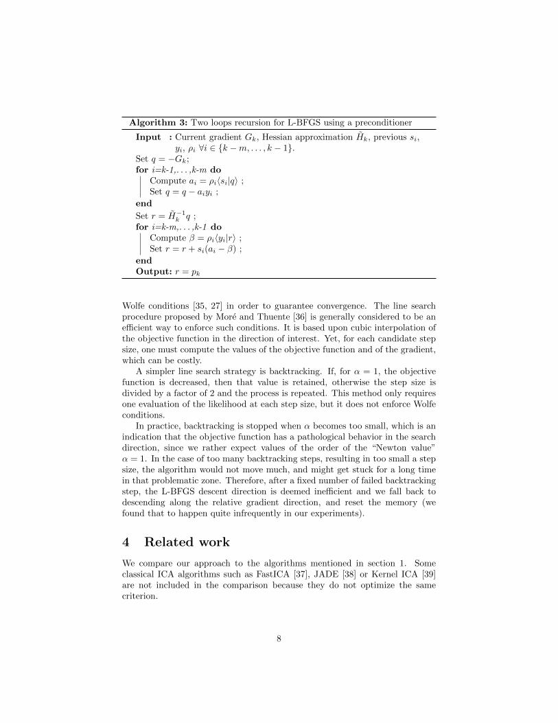
Algorithm 3: Two loops recursion for L-BFGS using a preconditioner
Input : Current gradient Gk, Hessian approximation Hk, previous si,yi, ρi ∀i ∈ {k −m, . . . , k − 1}.
Set q = −Gk;for i=k-1,. . . ,k-m do
Compute ai = ρi〈si|q〉 ;Set q = q − aiyi ;
end
Set r = H−1k q ;for i=k-m,. . . ,k-1 do
Compute β = ρi〈yi|r〉 ;Set r = r + si(ai − β) ;
endOutput: r = pk
Wolfe conditions [35, 27] in order to guarantee convergence. The line searchprocedure proposed by More and Thuente [36] is generally considered to be anefficient way to enforce such conditions. It is based upon cubic interpolation ofthe objective function in the direction of interest. Yet, for each candidate stepsize, one must compute the values of the objective function and of the gradient,which can be costly.
A simpler line search strategy is backtracking. If, for α = 1, the objectivefunction is decreased, then that value is retained, otherwise the step size isdivided by a factor of 2 and the process is repeated. This method only requiresone evaluation of the likelihood at each step size, but it does not enforce Wolfeconditions.
In practice, backtracking is stopped when α becomes too small, which is anindication that the objective function has a pathological behavior in the searchdirection, since we rather expect values of the order of the “Newton value”α = 1. In the case of too many backtracking steps, resulting in too small a stepsize, the algorithm would not move much, and might get stuck for a long timein that problematic zone. Therefore, after a fixed number of failed backtrackingstep, the L-BFGS descent direction is deemed inefficient and we fall back todescending along the relative gradient direction, and reset the memory (wefound that to happen quite infrequently in our experiments).
4 Related work
We compare our approach to the algorithms mentioned in section 1. Someclassical ICA algorithms such as FastICA [37], JADE [38] or Kernel ICA [39]are not included in the comparison because they do not optimize the samecriterion.
8
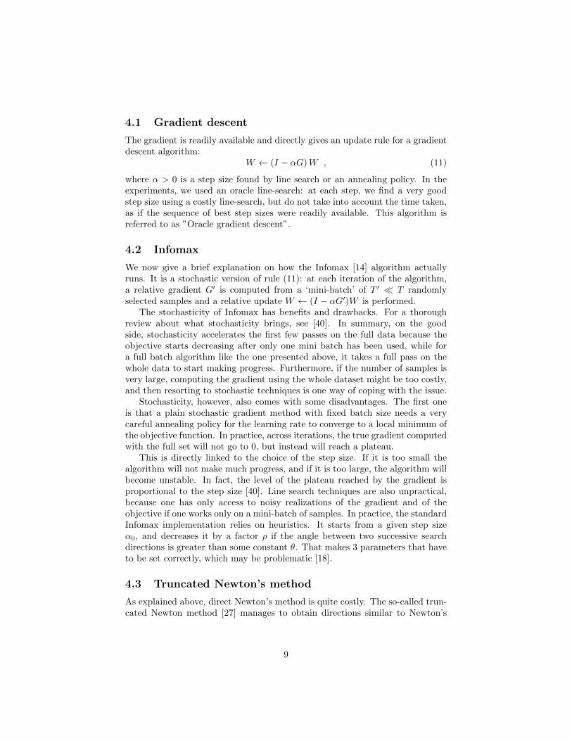
4.1 Gradient descent
The gradient is readily available and directly gives an update rule for a gradientdescent algorithm:
W ← (I − αG)W , (11)
where α > 0 is a step size found by line search or an annealing policy. In theexperiments, we used an oracle line-search: at each step, we find a very goodstep size using a costly line-search, but do not take into account the time taken,as if the sequence of best step sizes were readily available. This algorithm isreferred to as ”Oracle gradient descent”.
4.2 Infomax
We now give a brief explanation on how the Infomax [14] algorithm actuallyruns. It is a stochastic version of rule (11): at each iteration of the algorithm,a relative gradient G′ is computed from a ‘mini-batch’ of T ′ � T randomlyselected samples and a relative update W ← (I − αG′)W is performed.
The stochasticity of Infomax has benefits and drawbacks. For a thoroughreview about what stochasticity brings, see [40]. In summary, on the goodside, stochasticity accelerates the first few passes on the full data because theobjective starts decreasing after only one mini batch has been used, while fora full batch algorithm like the one presented above, it takes a full pass on thewhole data to start making progress. Furthermore, if the number of samples isvery large, computing the gradient using the whole dataset might be too costly,and then resorting to stochastic techniques is one way of coping with the issue.
Stochasticity, however, also comes with some disadvantages. The first oneis that a plain stochastic gradient method with fixed batch size needs a verycareful annealing policy for the learning rate to converge to a local minimum ofthe objective function. In practice, across iterations, the true gradient computedwith the full set will not go to 0, but instead will reach a plateau.
This is directly linked to the choice of the step size. If it is too small thealgorithm will not make much progress, and if it is too large, the algorithm willbecome unstable. In fact, the level of the plateau reached by the gradient isproportional to the step size [40]. Line search techniques are also unpractical,because one has only access to noisy realizations of the gradient and of theobjective if one works only on a mini-batch of samples. In practice, the standardInfomax implementation relies on heuristics. It starts from a given step sizeα0, and decreases it by a factor ρ if the angle between two successive searchdirections is greater than some constant θ. That makes 3 parameters that haveto be set correctly, which may be problematic [18].
4.3 Truncated Newton’s method
As explained above, direct Newton’s method is quite costly. The so-called trun-cated Newton method [27] manages to obtain directions similar to Newton’s
9
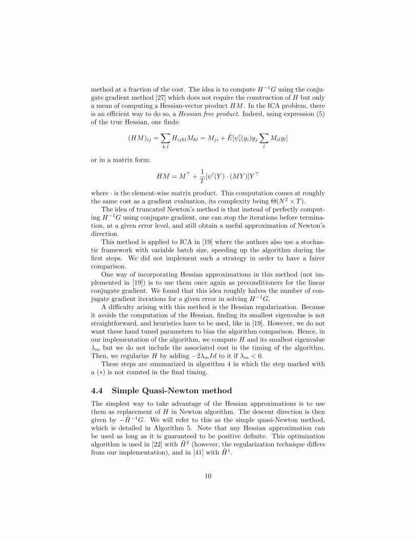
method at a fraction of the cost. The idea is to compute H−1G using the conju-gate gradient method [27] which does not require the construction of H but onlya mean of computing a Hessian-vector product HM . In the ICA problem, thereis an efficient way to do so, a Hessian free product. Indeed, using expression (5)of the true Hessian, one finds:
(HM)ij =∑k,l
HijklMkl = Mji + E[ψ′i(yi)yj∑l
Milyl]
or in a matrix form:
HM = M> +1
T[ψ′(Y ) · (MY )]Y >
where · is the element-wise matrix product. This computation comes at roughlythe same cost as a gradient evaluation, its complexity being Θ(N2 × T ).
The idea of truncated Newton’s method is that instead of perfectly comput-ing H−1G using conjugate gradient, one can stop the iterations before termina-tion, at a given error level, and still obtain a useful approximation of Newton’sdirection.
This method is applied to ICA in [19] where the authors also use a stochas-tic framework with variable batch size, speeding up the algorithm during thefirst steps. We did not implement such a strategy in order to have a fairercomparison.
One way of incorporating Hessian approximations in this method (not im-plemented in [19]) is to use them once again as preconditioners for the linearconjugate gradient. We found that this idea roughly halves the number of con-jugate gradient iterations for a given error in solving H−1G.
A difficulty arising with this method is the Hessian regularization. Becauseit avoids the computation of the Hessian, finding its smallest eigenvalue is notstraightforward, and heuristics have to be used, like in [19]. However, we do notwant these hand tuned parameters to bias the algorithm comparison. Hence, inour implementation of the algorithm, we compute H and its smallest eigenvalueλm but we do not include the associated cost in the timing of the algorithm.Then, we regularize H by adding −2λmId to it if λm < 0.
These steps are summarized in algorithm 4 in which the step marked witha (∗) is not counted in the final timing.
4.4 Simple Quasi-Newton method
The simplest way to take advantage of the Hessian approximations is to usethem as replacement of H in Newton algorithm. The descent direction is thengiven by −H−1G. We will refer to this as the simple quasi-Newton method,which is detailed in Algorithm 5. Note that any Hessian approximation canbe used as long as it is guaranteed to be positive definite. This optimizationalgorithm is used in [22] with H2 (however, the regularization technique differsfrom our implementation), and in [41] with H1.
10
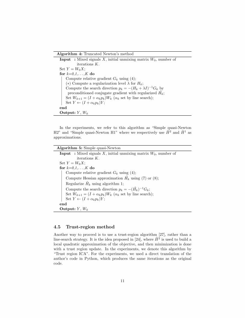
Algorithm 4: Truncated Newton’s method
Input : Mixed signals X, initial unmixing matrix W0, number ofiterations K.
Set Y = W0X;for k=0,1,. . . ,K do
Compute relative gradient Gk using (4);(∗) Compute a regularization level λ for Hk;Compute the search direction pk = −(Hk + λI)−1Gk bypreconditioned conjugate gradient with regularized Hk;
Set Wk+1 = (I + αkpk)Wk (αk set by line search);Set Y ← (I + αkpk)Y ;
endOutput: Y , Wk
In the experiments, we refer to this algorithm as “Simple quasi-NewtonH2” and “Simple quasi-Newton H1” where we respectively use H2 and H1 asapproximations.
Algorithm 5: Simple quasi-Newton
Input : Mixed signals X, initial unmixing matrix W0, number ofiterations K.
Set Y = W0X;for k=0,1,. . . ,K do
Compute relative gradient Gk using (4);
Compute Hessian approximation Hk using (7) or (8);
Regularize Hk using algorithm 1;
Compute the search direction pk = −(Hk)−1Gk;Set Wk+1 = (I + αkpk)Wk (αk set by line search);Set Y ← (I + αkpk)Y ;
endOutput: Y , Wk
4.5 Trust-region method
Another way to proceed is to use a trust-region algorithm [27], rather than aline-search strategy. It is the idea proposed in [24], where H2 is used to build alocal quadratic approximation of the objective, and then minimization is donewith a trust region update. In the experiments, we denote this algorithm by“Trust region ICA”. For the experiments, we used a direct translation of theauthor’s code in Python, which produces the same iterations as the originalcode.
11
5 Experiments
We went to great lengths to ensure a fair comparison of the above algorithms.We reimplemented each algorithm using the Python programming language.Since the most costly operations are by far those scaling with the number ofsamples (i.e. evaluations of the likelihood, score and its derivative, gradient,Hessian approximations and Hessian free products), we made sure that all im-plementations call the same functions, thereby ensuring that differences in con-vergence speed are caused by algorithmic differences rather than by details ofimplementation.
Our implementations of Picard, the simple quasi-Newton method, the trun-cated Newton method and the trust region method are available online1.
5.1 Experimental setup
All the following experiments have been performed on the same computer usingonly one core of an Intel Core i7-6600U @ 2.6 GHz. For optimized numericalcode we relied on Numpy [42] using Intel MKL as the linear algebra backendlibrary, and the numexpr package2 to optimize CPU cache. It was particularlyefficient in computing log cosh(yi(t)/2) and tanh(yi(t)/2) ∀i, t.
For each ICA experiment, we keep track of the gradient infinite norm (definedas maxij |Gij |) across time and across iterations. The algorithms are stoppedif a certain predefined number of iterations is exceeded or if the gradient normreaches a small threshold (typically 10−8).
Each experiment is repeated a certain number of times to increase the ro-bustness of the conclusions. We end up with several gradient norm curves. Onthe convergence plots, we only display the median of these curves to maintainreadability: half experiments finished faster and the other half finished slowerthan the plotted curve.
Besides the algorithms mentioned above, we have run a vanilla version ofthe L-BFGS algorithm, and Picard algorithm using H1 and H2.
5.2 Preprocessing
A standard preprocessing for ICA is applied in all our experiments, as follows.Any given input matrix X is first mean-corrected by subtracting to each row itsmean value. Next, the data are whitened by multiplication by a matrix inversesquare root of the empirical covariance matrix C = 1
TXX>. After whitening,
the covariance matrix of the transformed signals is the identity matrix. In otherwords, the signals are decorrelated and scaled to unit variance.
1https://github.com/pierreablin/faster-ica2 https://github.com/pydata/numexpr
12
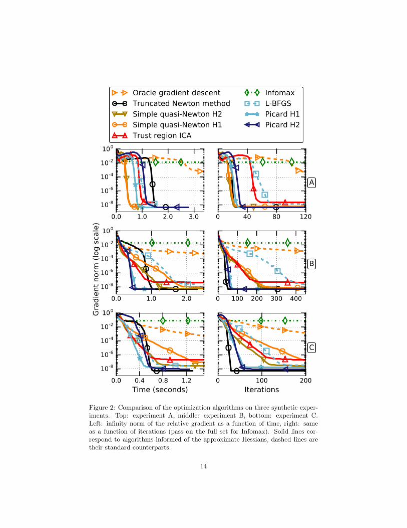
5.3 Simulation study
In this first study, we present results obtained on synthetic data. The generalsetup is the following: we choose the number of sources N , the number ofsamples T and a probability density for each source. For each of the N densities,we draw T independent samples. Then, a random mixing matrix whose entriesare normally distributed with zero mean and unit variance is created. Thesynthetic signals are obtained by multiplying the source signals by the mixingmatrix and preprocessed as described in section (5.2).
We repeat the experiments 100 times, changing for each run the seed gener-ating the random signals.
We considerd 3 different setups:
• Experiment A: T = 10000 independent samples of N = 50 independentsources. All sources are drawn with the same density p(x) = 1
2 exp(−|x|).
• Experiment B : T = 10000 independent samples of N = 15 indepen-dent sources. The 5 first sources have density p(x) = exp(−|x|), the 5next sources are Gaussian, and the 5 last sources have density p(x) ∝exp(−|x3|).
• Experiment C : T = 5000 independent samples of N = 40 independentsources. The ith source has density pi = αiN (0, 1) + (1 − αi)N (0, σ2)where σ = 0.1 and αi is a sequence of linearly spaced values betweenα1 = 0.5 and αn = 1.
In experiment A, the ICA assumption holds perfectly, and each source hasa super Gaussian density, for which the choice ψ = tanh(·/2) is appropriate.In experiment B, the first 5 sources can be recovered by the algorithms for thesame reason. However, the next 5 sources cannot because they are Gaussian,and the last 5 sources cannot be recovered either because they are sub-Gaussian.Finally, in experiment C, the mixture is identifiable but, because of the limitednumber of samples, the most Gaussian sources cannot be distinguished froman actual Gaussian signal. The results of the three experiments are shown inFigure 2.
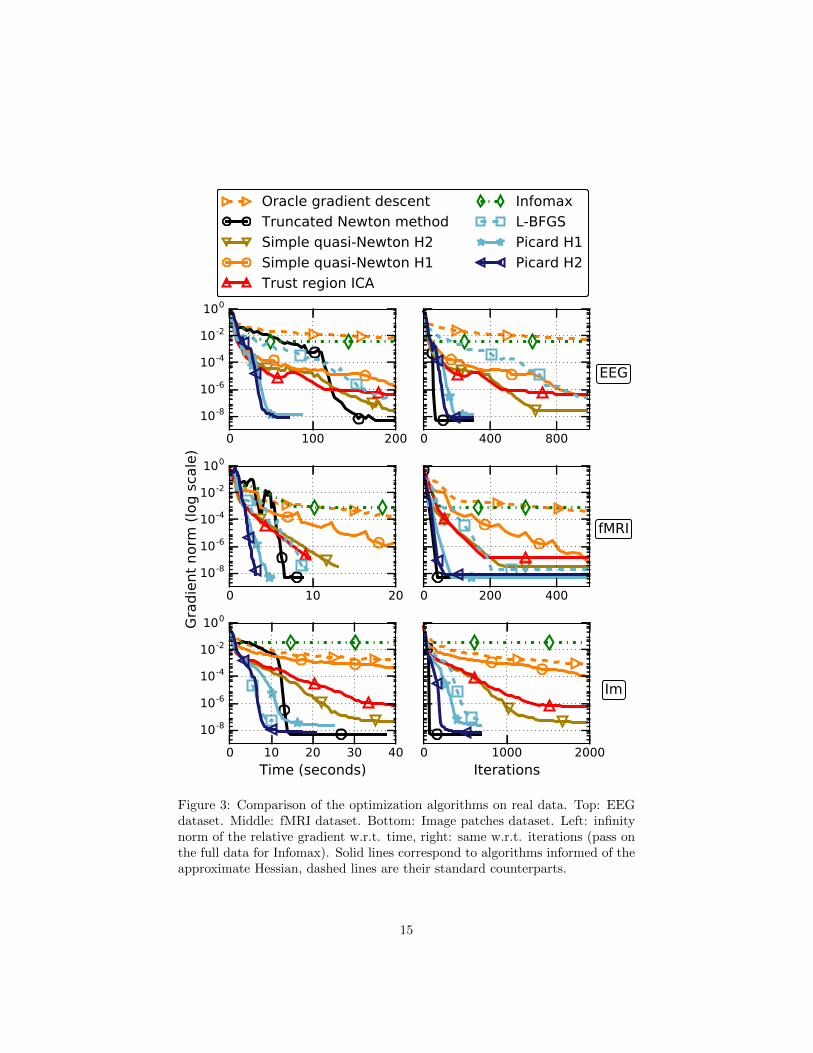
5.4 Experiments on EEG data
Our algorithms were also run on 13 publicly available3 EEG datasets [6]. Eachrecording contains n = 71 signals, and has been down-sampled by 4 for a finallength of T ' 75000 samples. EEG measures the changes of electric potentialinduced by brain activity. For such data, the ICA assumption does not per-fectly hold. In addition, brain signals are contaminated by a lot of noise andartifacts. Still, it has been shown that ICA succeeds at extracting meaningfuland biologically plausible sources from these mixtures [43, 3, 6]. Results aredisplayed on the top row of Figure 3.
3https://sccn.ucsd.edu/wiki/BSSComparison
13
0.0 1.0 2.0 3.0
10-8
10-6
10-4
10-2
100
0 40 80 120
0.0 1.0 2.0
10-8
10-6
10-4
10-2
100
0 100 200 300 400
0.0 0.4 0.8 1.2
Time (seconds)
10-8
10-6
10-4
10-2
100
0 100 200
Iterations
Oracle gradient descent
Truncated Newton method
Simple quasi-Newton H2
Simple quasi-Newton H1
Trust region ICA
Infomax
L-BFGS
Picard H1
Picard H2
Gra
die
nt
norm
(lo
g s
cale
)
A
B
C
Figure 2: Comparison of the optimization algorithms on three synthetic exper-iments. Top: experiment A, middle: experiment B, bottom: experiment C.Left: infinity norm of the relative gradient as a function of time, right: sameas a function of iterations (pass on the full set for Infomax). Solid lines cor-respond to algorithms informed of the approximate Hessians, dashed lines aretheir standard counterparts.
14
0 100 200
10-8
10-6
10-4
10-2
100
Oracle gradient descent
Truncated Newton method
Simple quasi-Newton H2
Simple quasi-Newton H1
Trust region ICA
Infomax
L-BFGS
Picard H1
Picard H2
0 400 800
Oracle gradient descent
Truncated Newton method
Simple quasi-Newton H2
Simple quasi-Newton H1
Trust region ICA
Infomax
L-BFGS
Picard H1
Picard H2
0 10 20
10-8
10-6
10-4
10-2
100
0 200 400
0 10 20 30 40
Time (seconds)
10-8
10-6
10-4
10-2
100
0 1000 2000
Iterations
Gra
die
nt
norm
(lo
g s
cale
)
EEG
fMRI
Im
Figure 3: Comparison of the optimization algorithms on real data. Top: EEGdataset. Middle: fMRI dataset. Bottom: Image patches dataset. Left: infinitynorm of the relative gradient w.r.t. time, right: same w.r.t. iterations (pass onthe full data for Infomax). Solid lines correspond to algorithms informed of theapproximate Hessian, dashed lines are their standard counterparts.
15
5.5 Experiments on fMRI data
For those experiments, we used preprocessed fMRI data from the ADHD-200consortium [44]. We perform group ICA using the CanICA framework [45] inNilearn [46]. From the fMRI data of several patients, CanICA builds a signalmatrix to which classical ICA is applied. We use that matrix to benchmark thealgorithms. The problem is of size N = 40 and T ' 60000. See middle row ofFigure 3.
5.6 Experiments on natural images
Given a grayscale image, we extract T square patches (contiguous squares ofpixels) of size (s, s). Each patch is vectorized, yielding an s2 × T data matrix.One may compute an ICA of this data set and see the columns of the mixingmatrix W−1 as features, or dictionary atoms, learned from random patches.
The ICA algorithms are run on a set of 100 natural images of open coun-try4 [47], using T = 30000 patches of side 8× 8 pixels, resulting in a 64× 30000data matrix. The patches are all centered and scaled so that their mean andvariance equal 0 and 1 respectively before whitening as in section 5.2. Resultsare shown at the bottom of Figure 3.
5.7 Discussion
On the first synthetic experiment, where the ICA mixture model holds, secondorder algorithms are all seen to perform well, converging in a handful of iter-ations. For this problem, the fastest algorithms are the simple quasi-Newtonmethods, which means that Picard does not improve significantly over the Hes-sian approximations H1 or H2. This is expected since the Hessian approxima-tions are very efficient when the ICA mixture model holds.
On the two other simulations, the ICA model is not identifiable because ofthe Gaussian signals. First order methods perform poorly. We can observe thatfor algorithms relying only on the Hessian approximations (simple quasi-Newtonand trust-region ICA), the convergence speed is reduced. On the contrary,Picard and truncated Newton manage to keep a very quick convergence. Onthose synthetic problems, it is not clear whether or not the greater accuracy ofH2 over H1 justifies the added computation cost.
On EEG and fMRI data, Picard still converges quickly, in a fraction of thetime taken by the other algorithms. For this problem, using H2 for precondi-tioning leads to faster convergence than H1. The results are even more strikingon images, where Picard, standard L-BFGS and truncated Newton converge ina few seconds while the other algorithms show a very slow linear convergencepattern.
On all experiments, truncated Newton’s method converges in fewer iterationsthan Picard. This happens because it follows a direction very close to Newton’strue direction, which is the direction each second order algorithm tries to mimic
4http://cvcl.mit.edu/database.htm
16
when the current iterate is close to the optimum. However, if we comparealgorithms in terms of time, the picture is different: the reduced number ofiterations does not make up for the added cost compared to Picard.
5.8 Complexity comparison of truncated Newton and pre-conditioned L-BFGS
Truncated Newton’s method uses the full information about the curvature. Inour experiments, we observe that while this method converges in fewer itera-tions than Picard, it is slower in terms of CPU time. The speed of truncatedNewton depends on many parameters (stopping policy for the conjugate gra-dient, regularization of H and of H), so we propose a complexity comparisonof this algorithm and Picard, to understand if the former might sometimes befaster than the latter.
Operations carried by the algorithms fall into two categories. First, thereare operations that do not scale with the number of samples T , but only withthe number of sources N . Regularizing the Hessian, computing H−1G and theL-BFGS inner loop are such operations. The remaining operations scale linearlywith T . Computing the score, its derivative, or evaluating the likelihood are allθ(N × T ) operations. The most costly operations are in Θ(N2 × T ). They are:
computing the gradient, computing H2, and for the truncated Newton method,computing a Hessian free product.
For the following study, let us reason in the context where T is large in frontof N2, as it is the case for most real data applications. In that context, we donot count operations not scaling with T . This is a reasonable assumption onreal datasets: on the EEG problem, these operations make for less than 1% ofthe total timing for Picard.
To keep the analysis simple, let us also assume that the operations in Θ(N×T ) are negligible in front of those in Θ(N2×T ). When computing a gradient, thecoefficients of H2 or a Hessian free product, the costly operation in Θ(N2 × T )is numerically the same: it is the computation of a matrix product of the formY1Y
>2 where Y1 and Y2 have the same shape as Y . With that in mind, we
assume that each of these operations take the same time, tG.In order to produce a descent direction, Picard only needs the current gra-
dient and Hessian approximations; the remaining operations do not scale withT . This means that each descent direction takes about 2× tG to be found. Thiscomplexity is exactly the same as the simple quasi-Newton method. On theother hand, truncated Newton requires the two same operations, as well as oneHessian-free product for each inner iteration of the conjugate gradient. If wedenote by Ncg the number of inner loops for the conjugate gradient, we find thattruncated Newton’s method takes (2 +Ncg)× tG to find the descent direction.
Now, in our experiments, we can see that truncated Newton converges inabout half as many iterations as Picard. Hence, for truncated Newton to becompetitive, each of its iterations should take no longer than twice a Picarditeration. That would require Ncg ≤ 2 but in practice, we observed that many
17
more conjugate gradient iterations are needed (usually more than 10) to providea satisfying Newton direction. On the other hand, if the conjugate gradientalgorithm is allowed to perform only Ncg = 2 inner loops at each iteration, itresults in a direction which is far from Newton’s direction, drastically increasingthe number of iterations required for convergence.
This analysis leads us to think that the truncated Newton’s method as de-scribed in section 4.3 cannot be faster than Picard.
5.9 Study of the control parameters of Picard
Picard has four control parameters: binary choice between two Hessian ap-proximations, memory size m for L-BFGS, number nls of tries allowed for thebacktracking line-search and regularization constant λmin. Our experiments in-dicate that H2 is overall a better preconditioner for the algorithm, although thedifference with H1 can be small.
Through experiments, we found that the memory size had barely no effectin the range 3 ≤ m ≤ 15. For a smaller value of m, the algorithm does not haveenough information to build a good Hessian approximation. If m is too large,the Hessian built by the algorithm is biased by the landscape explored too farin the past.
The number of tries for the line-search has a tangible effect on convergencespeed. Similarly, the optimal regularization constant depends on the difficultyof the problem. However, on the variety of different signals processed in ourexperiments (synthetic, EEG, fMRI and image), we used the same parametersm = 7, nls = 10 and λmin = 10−2. As reported, those values yielded uniformlygood performance.
6 Conclusion
While ICA is massively used across scientific domains, computation time forinference can be a bottleneck in many applications. The purpose of this workwas to design a fast and accurate algorithm for maximum-likelihood ICA.
For this optimization problem, there are computationally cheap approxima-tions of the Hessian. This leads to simple quasi-Newton algorithms that havea cost per iteration only twice as high as a gradient descent, while offering farbetter descent directions. Yet, such approximations can be far from the trueHessian on real datasets. As a consequence, practical convergence is not asfast as one can expect from a second order method. Another approach is touse a truncated Newton algorithm, which yields directions closer to Newton’salgorithm, but at a much higher cost per iteration.
In this work, we introduced the Preconditioned ICA for Real Data (Picard)algorithm, which combines both ideas. We use the Hessian approximations aspreconditioners for the L-BFGS method. The algorithm refines the Hessianapproximations to better take into account the true curvature. The cost per
18
iteration of Picard is similar to the simple quasi-Newton methods, while pro-viding far better descent directions. This was demonstrated, through carefulimplementation of various literature methods and extensive experiments oversynthetic, EEG, fMRI and image data, where we showed clear gains in runningtime compared to the state-of-the-art.
Future work
The algorithm presented in this article is developed with fixed score functions. Itwould be of interest to extend it to an adaptive score framework for the recoveryof a broader class of sources. An option is to alternate steps of mixing matrixestimation and steps of density estimation, as is done in AMICA for instance. Inpreliminary experiments, such an approach was found to impair the convergencespeed of the algorithm. More evolved methods have to be considered.
Second, the regularization technique presented here is based on a trial anderror heuristic which has worked uniformly well on each studied dataset. Still,since the eigenvalues of the Hessian are driven by the statistics of the signals, acareful study might lead to more informed regularization strategies.
Acknowledgments
This work was supported by the Center for Data Science, funded by the IDEXParis-Saclay, ANR-11-IDEX-0003-02, and the European Research Council (ERCSLAB-YStG-676943).
Acknowledgment
This work was supported by the Center for Data Science, funded by the IDEXParis-Saclay, ANR-11-IDEX-0003-02, and the European Research Council (ERCSLAB-YStG-676943).
References
[1] P. Comon, “Independent component analysis, a new concept?” Signal Pro-cessing, vol. 36, no. 3, pp. 287 – 314, 1994.
[2] A. Hyvarinen and E. Oja, “Independent component analysis: algorithmsand applications,” Neural networks, vol. 13, no. 4, pp. 411–430, 2000.
[3] S. Makeig, T.-P. Jung, A. J. Bell, D. Ghahremani, and T. J. Sejnowski,“Blind separation of auditory event-related brain responses into inde-pendentcomponents,” Proceedings of the National Academy of Sciences(PNAS), vol. 94, no. 20, pp. 10 979–10 984, 1997.
19
[4] V. Calhoun, T. Adali, G. Pearlson, and J. Pekar, “A method for makinggroup inferences from functional MRI data using independent componentanalysis,” Human Brain Mapping, vol. 14, no. 3, pp. 140–151, 2001.
[5] C. F. Beckmann and S. M. Smith, “Probabilistic independent componentanalysis for functional magnetic resonance imaging,” IEEE Transactionson Medical Imaging, vol. 23, no. 2, pp. 137–152, Feb 2004.
[6] A. Delorme, J. Palmer, J. Onton, R. Oostenveld, and S. Makeig, “Indepen-dent EEG sources are dipolar,” PloS one, vol. 7, no. 2, p. e30135, 2012.
[7] D. Nuzillard and A. Bijaoui, “Blind source separation and analysis of mul-tispectral astronomical images,” Astronomy and Astrophysics SupplementSeries, vol. 147, no. 1, pp. 129–138, 2000.
[8] D. Maino, A. Farusi, C. Baccigalupi, F. Perrotta, A. Banday, L. Bedini,C. Burigana, G. De Zotti, K. Gorski, and E. Salerno, “All-sky astrophysi-cal component separation with fast independent component analysis (FAS-TICA),” Monthly Notices of the Royal Astronomical Society, vol. 334, no. 1,pp. 53–68, 2002.
[9] A. Cadavid, J. Lawrence, and A. Ruzmaikin, “Principal components andindependent component analysis of solar and space data,” Solar Physics,vol. 248, no. 2, pp. 247–261, 2008.
[10] V. Vrabie, C. Gobinet, O. Piot, A. Tfayli, P. Bernard, R. Huez, andM. Manfait, “Independent component analysis of raman spectra: Appli-cation on paraffin-embedded skin biopsies,” Biomedical Signal Processingand Control, vol. 2, no. 1, pp. 40 – 50, 2007.
[11] D. N. Rutledge and D. J.-R. Bouveresse, “Independent components analysiswith the JADE algorithm,” TrAC Trends in Analytical Chemistry, vol. 50,pp. 22–32, 2013.
[12] S.-I. Lee and S. Batzoglou, “Application of independent component analysisto microarrays,” Genome biology, vol. 4, no. 11, p. R76, 2003.
[13] M. Scholz, S. Gatzek, A. Sterling, O. Fiehn, and J. Selbig, “Metabolite fin-gerprinting: detecting biological features by independent component anal-ysis,” Bioinformatics, vol. 20, no. 15, pp. 2447–2454, 2004.
[14] A. J. Bell and T. J. Sejnowski, “An information-maximization approachto blind separation and blind deconvolution,” Neural computation, vol. 7,no. 6, pp. 1129–1159, 1995.
[15] A. Delorme and S. Makeig, “EEGLAB: an open source toolbox for analysisof single-trial EEG dynamics including independent component analysis,”Journal of neuroscience methods, vol. 134, no. 1, pp. 9–21, 2004.
20
[16] A. Gramfort, M. Luessi, E. Larson, D. A. Engemann, D. Strohmeier,C. Brodbeck, L. Parkkonen, and M. S. Hmlinen, “MNE software for pro-cessing MEG and EEG data,” NeuroImage, vol. 86, pp. 446 – 460, 2014.
[17] J.-F. Cardoso, “Infomax and maximum likelihood for blind source separa-tion,” IEEE Signal processing letters, vol. 4, no. 4, pp. 112–114, 1997.
[18] J. Montoya-Martınez, J.-F. Cardoso, and A. Gramfort, “Caveats withstochastic gradient and maximum likelihood based ICA for EEG,” in In-ternational Conference on Latent Variable Analysis and Signal Separation.Springer, 2017, pp. 279–289.
[19] P. Tillet, H. Kung, and D. Cox, “Infomax-ICA using hessian-free optimiza-tion,” in Acoustics, Speech and Signal Processing (ICASSP), 2017 IEEEInternational Conference on. IEEE, 2017, pp. 2537–2541.
[20] D. T. Pham and P. Garat, “Blind separation of mixture of independentsources through a quasi-maximum likelihood approach,” IEEE Transac-tions on Signal Processing, vol. 45, no. 7, pp. 1712–1725, 1997.
[21] S.-I. Amari, T.-P. Chen, and A. Cichocki, “Stability analysis of learningalgorithms for blind source separation,” Neural Networks, vol. 10, no. 8,pp. 1345–1351, 1997.
[22] M. Zibulevsky, “Blind source separation with relative newton method,” inProc. ICA, vol. 2003, 2003, pp. 897–902.
[23] J. A. Palmer, S. Makeig, K. Kreutz-Delgado, and B. D. Rao, “Newtonmethod for the ICA mixture model,” in IEEE International Conferenceon Acoustics, Speech and Signal Processing (ICASSP), March 2008, pp.1805–1808.
[24] H. Choi and S. Choi, “A relative trust-region algorithm for independentcomponent analysis,” Neurocomputing, vol. 70, no. 7, pp. 1502–1510, 2007.
[25] R. H. Byrd, P. Lu, J. Nocedal, and C. Zhu, “A limited memory algorithmfor bound constrained optimization,” SIAM Journal on Scientific Comput-ing, vol. 16, no. 5, pp. 1190–1208, 1995.
[26] J.-F. Cardoso and B. H. Laheld, “Equivariant adaptive source separation,”IEEE Transactions on Signal Processing, vol. 44, no. 12, pp. 3017–3030,1996.
[27] J. Nocedal and S. J. Wright, Numerical Optimization. Springer, 1999.
[28] W. C. Davidon, “Variable metric method for minimization,” SIAM Journalon Optimization, vol. 1, no. 1, pp. 1–17, 1991.
[29] R. Fletcher, “A new approach to variable metric algorithms,” The computerjournal, vol. 13, no. 3, pp. 317–322, 1970.
21
[30] R. Fletcher and M. J. Powell, “A rapidly convergent descent method forminimization,” The computer journal, vol. 6, no. 2, pp. 163–168, 1963.
[31] C. G. Broyden, “The convergence of a class of double-rank minimization al-gorithms 1. general considerations,” IMA Journal of Applied Mathematics,vol. 6, no. 1, pp. 76–90, 1970.
[32] D. Goldfarb, “A family of variable-metric methods derived by variationalmeans,” Mathematics of computation, vol. 24, no. 109, pp. 23–26, 1970.
[33] D. F. Shanno, “Conditioning of quasi-newton methods for function min-imization,” Mathematics of computation, vol. 24, no. 111, pp. 647–656,1970.
[34] L. Jiang, R. H. Byrd, E. Eskow, and R. B. Schnabel, “A preconditionedL-BFGS algorithm with application to molecular energy minimization,”Colorado Univ. at Boulder Dept. of Computer Science, Tech. Rep., 2004.
[35] P. Wolfe, “Convergence conditions for ascent methods,” SIAM review,vol. 11, no. 2, pp. 226–235, 1969.
[36] J. J. More and D. J. Thuente, “Line search algorithms with guaranteed suf-ficient decrease,” ACM Transactions on Mathematical Software (TOMS),vol. 20, no. 3, pp. 286–307, 1994.
[37] A. Hyvarinen, “Fast and robust fixed-point algorithms for independentcomponent analysis,” IEEE Transactions on Neural Networks, vol. 10,no. 3, pp. 626–634, 1999.
[38] J. F. Cardoso and A. Souloumiac, “Blind beamforming for non-gaussiansignals,” IEE Proceedings F - Radar and Signal Processing, vol. 140, no. 6,pp. 362–370, Dec 1993.
[39] F. R. Bach and M. I. Jordan, “Kernel independent component analysis,”Journal of machine learning research, vol. 3, no. Jul, pp. 1–48, 2002.
[40] L. Bottou, F. E. Curtis, and J. Nocedal, “Optimization methods for large-scale machine learning,” arXiv preprint arXiv:1606.04838, 2016.
[41] J. A. Palmer, K. Kreutz-Delgado, and S. Makeig, “AMICA: An adaptivemixture of independent component analyzers with shared components,”Tech. Rep., 2012.
[42] S. Van der Walt, S. Colbert, and G. Varoquaux, “The NumPy array:a structure for efficient numerical computation,” Comp. in Sci. & Eng.,vol. 13, no. 2, pp. 22–30, 2011.
[43] T.-P. Jung, C. Humphries, T.-W. Lee, S. Makeig, M. J. McKeown,V. Iragui, and T. J. Sejnowski, “Extended ICA removes artifacts fromelectroencephalographic recordings,” in Proceedings of the 10th Interna-tional Conference on Neural Information Processing Systems, ser. NIPS’97.Cambridge, MA, USA: MIT Press, 1997, pp. 894–900.
22
[44] A.-. Consortium et al., “The ADHD-200 consortium: a model to advancethe translational potential of neuroimaging in clinical neuroscience,” Fron-tiers in systems neuroscience, vol. 6, 2012.
[45] G. Varoquaux, S. Sadaghiani, P. Pinel, A. Kleinschmidt, J.-B. Poline,and B. Thirion, “A group model for stable multi-subject ICA on fMRIdatasets,” Neuroimage, vol. 51, no. 1, pp. 288–299, 2010.
[46] A. Abraham, F. Pedregosa, M. Eickenberg, P. Gervais, A. Mueller, J. Kos-saifi, A. Gramfort, B. Thirion, and G. Varoquaux, “Machine learning forneuroimaging with scikit-learn,” Frontiers in neuroinformatics, vol. 8, 2014.
[47] A. Oliva and A. Torralba, “Modeling the shape of the scene: A holisticrepresentation of the spatial envelope,” International journal of computervision, vol. 42, no. 3, pp. 145–175, 2001.
23