Embed Size (px)
Citation preview
Incremental Learning via Rate Reduction
Kyung Eun BaekYi Ma
Electrical Engineering and Computer SciencesUniversity of California, Berkeley
Technical Report No. UCB/EECS-2021-130
http://www2.eecs.berkeley.edu/Pubs/TechRpts/2021/EECS-2021-130.html
May 14, 2021

Copyright © 2021, by the author(s).All rights reserved.
Permission to make digital or hard copies of all or part of this work forpersonal or classroom use is granted without fee provided that copies arenot made or distributed for profit or commercial advantage and that copiesbear this notice and the full citation on the first page. To copy otherwise, torepublish, to post on servers or to redistribute to lists, requires prior specificpermission.
Incremental Learning via Rate Reduction
by Christina Baek
Research Project
Submitted to the Department of Electrical Engineering and Computer Sciences, University of California at Berkeley, in partial satisfaction of the requirements for the degree of Master of Science, Plan II. Approval for the Report and Comprehensive Examination:
Committee:
Professor Yi Ma Research Advisor
(Date)
* * * * * * *
Professor Anant Sahai Second Reader
(Date)
May 13, 2021
Incremental Learning via Rate Reduction
by
Christina Baek
A thesis submitted in partial satisfaction of the
requirements for the degree of
Master of Science
in
Electrical Engineering and Computer Science
in the
Graduate Division
of the
University of California, Berkeley
Committee in charge:
Professor Yi Ma, ChairProfessor Anant Sahai
Spring 2021
1
Abstract
Incremental Learning via Rate Reduction
by
Christina Baek
Master of Science in Electrical Engineering and Computer Science
University of California, Berkeley
Professor Yi Ma, Chair
Current deep learning architectures suffer from catastrophic forgetting, a failure to retainknowledge of previously learned classes when incrementally trained on new classes. Thefundamental roadblock faced by deep learning methods is that the models are optimizedas “black boxes,” making it difficult to properly adjust the model parameters to preserveknowledge about previously seen data. To overcome the problem of catastrophic forgetting,we propose utilizing an alternative “white box” architecture derived from the principle of ratereduction, where each layer of the network is explicitly computed without back propagation.Under this paradigm, we demonstrate that, given a pretrained network and new data classes,our approach can provably construct a new network that emulates joint training with allpast and new classes. Finally, our experiments show that our proposed learning algorithmobserves significantly less decay in classification performance, outperforming state of the artmethods on MNIST and CIFAR-10 by a large margin and justifying the use of “white box”algorithms for incremental learning even for sufficiently complex image data.
i
Contents
Contents i
List of Figures ii
List of Tables iii
1 Interpretable Network from Rate Reduction 11.1 Principle of Maximal Coding Rate Reduction . . . . . . . . . . . . . . . . . 11.2 Rate Reduction Network (ReduNet) . . . . . . . . . . . . . . . . . . . . . . . 3
2 ReduNet for Interpretable Incremental Learning 52.1 Introduction . . . . . . . . . . . . . . . . . . . . . . . . . . . . . . . . . . . . 52.2 Related Work . . . . . . . . . . . . . . . . . . . . . . . . . . . . . . . . . . . 62.3 Incremental Learning with ReduNet . . . . . . . . . . . . . . . . . . . . . . . 82.4 Experiments . . . . . . . . . . . . . . . . . . . . . . . . . . . . . . . . . . . . 122.5 Conclusions and Future Work . . . . . . . . . . . . . . . . . . . . . . . . . . 16
3 Low Rank Approximation for Efficient ReduNet 173.1 Low rank approximation . . . . . . . . . . . . . . . . . . . . . . . . . . . . . 173.2 Block Diagonal Approximation by Eigenspace . . . . . . . . . . . . . . . . . 203.3 Conclusion . . . . . . . . . . . . . . . . . . . . . . . . . . . . . . . . . . . . . 25
Bibliography 26
ii
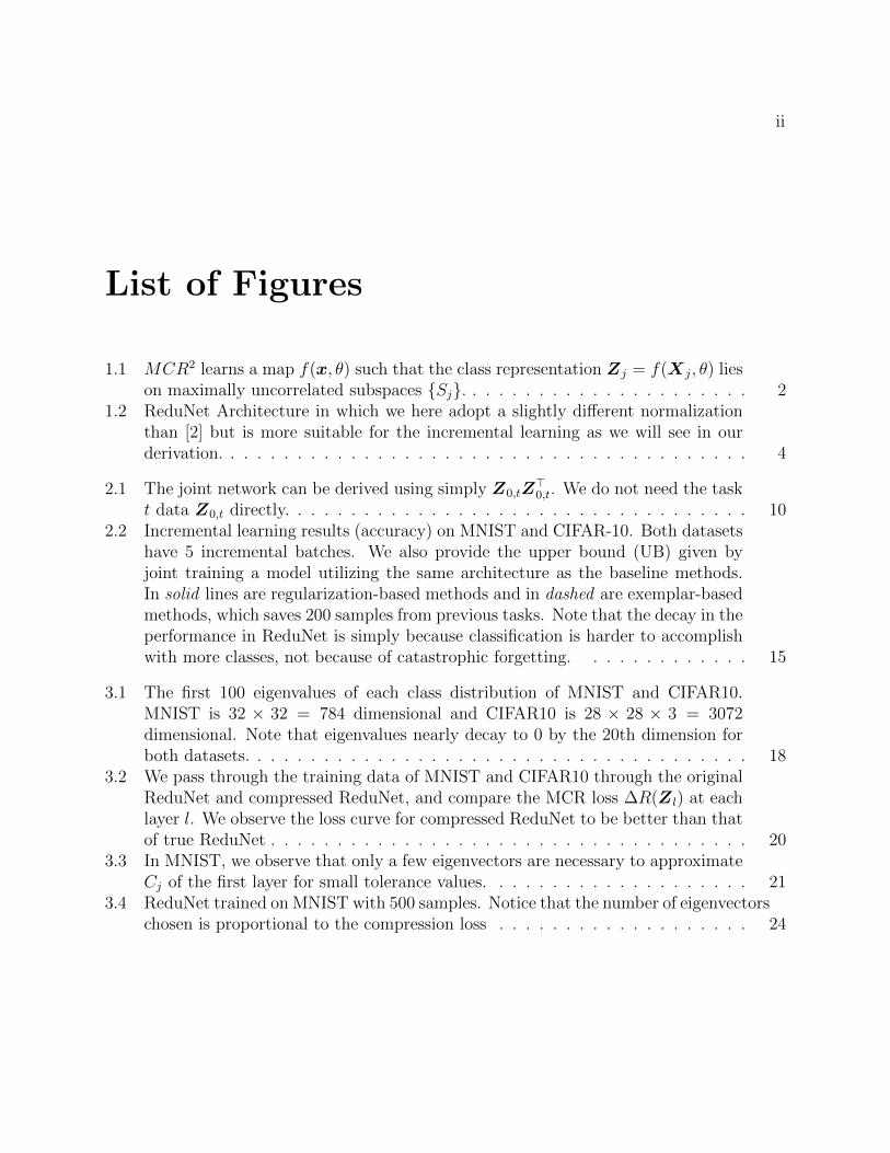
List of Figures
1.1 MCR2 learns a map f(x, θ) such that the class representation Zj = f(Xj, θ) lieson maximally uncorrelated subspaces {Sj}. . . . . . . . . . . . . . . . . . . . . . 2
1.2 ReduNet Architecture in which we here adopt a slightly different normalizationthan [2] but is more suitable for the incremental learning as we will see in ourderivation. . . . . . . . . . . . . . . . . . . . . . . . . . . . . . . . . . . . . . . . 4
2.1 The joint network can be derived using simply Z0,tZ>0,t. We do not need the task
t data Z0,t directly. . . . . . . . . . . . . . . . . . . . . . . . . . . . . . . . . . . 102.2 Incremental learning results (accuracy) on MNIST and CIFAR-10. Both datasets
have 5 incremental batches. We also provide the upper bound (UB) given byjoint training a model utilizing the same architecture as the baseline methods.In solid lines are regularization-based methods and in dashed are exemplar-basedmethods, which saves 200 samples from previous tasks. Note that the decay in theperformance in ReduNet is simply because classification is harder to accomplishwith more classes, not because of catastrophic forgetting. . . . . . . . . . . . . 15
3.1 The first 100 eigenvalues of each class distribution of MNIST and CIFAR10.MNIST is 32 × 32 = 784 dimensional and CIFAR10 is 28 × 28 × 3 = 3072dimensional. Note that eigenvalues nearly decay to 0 by the 20th dimension forboth datasets. . . . . . . . . . . . . . . . . . . . . . . . . . . . . . . . . . . . . . 18
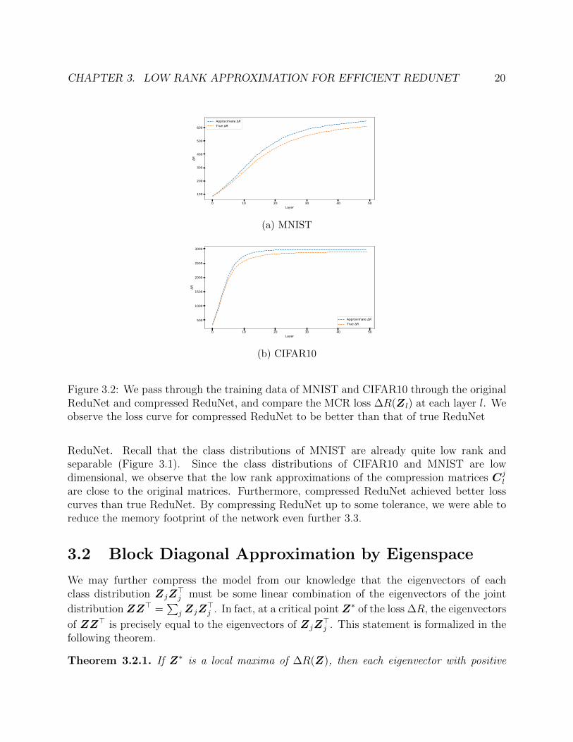
3.2 We pass through the training data of MNIST and CIFAR10 through the originalReduNet and compressed ReduNet, and compare the MCR loss ∆R(Z l) at eachlayer l. We observe the loss curve for compressed ReduNet to be better than thatof true ReduNet . . . . . . . . . . . . . . . . . . . . . . . . . . . . . . . . . . . . 20
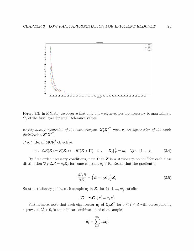
3.3 In MNIST, we observe that only a few eigenvectors are necessary to approximateCj of the first layer for small tolerance values. . . . . . . . . . . . . . . . . . . . 21
3.4 ReduNet trained on MNIST with 500 samples. Notice that the number of eigenvectorschosen is proportional to the compression loss . . . . . . . . . . . . . . . . . . . 24

iii
List of Tables
2.1 Test Accuracy (%) on Task 1 After Each Training Session on MNIST and CIFAR-10. 14

iv
Acknowledgments
This work was a joint effort with students Ziyang Wu and Chong You, advised by ProfessorYi Ma. I would like to thank Professor Yi Ma for the invaluable opportunities he has givenme this year to learn and grow as a student and researcher. I learned tremendously fromhim and graduate students Simon, Yaodong, Chong, Xili, and others, whose dedication andcompassion inspired me on a daily basis to keep working towards a better understandingof this field. I dedicate my thesis to my family, from whom I always receive unwaveringsupport.
1
Chapter 1
Interpretable Network from RateReduction
1.1 Principle of Maximal Coding Rate Reduction
Given a set of training data {xi} and their corresponding labels {yi}, classical deep learningaims to learn a nonlinear mapping h(·) : x → y, implemented as a series of simple linearand nonlinear maps, that minimizes the cross-entropy loss. One popular way to interpretthe role of multiple layers is to consider the output of each intermediate layer as a latentrepresentation space. Then, the beginning layers aim to learn a latent representation z =f(x, θ) ∈ Rd that best facilitates the later layers y = g(z) for the downstream classificationtask.
xf(x,θ)−−−→ z(θ)
g(z)−−→ y
As a concrete example, in image recognition tasks, f(·) is a convolutional backbone thatencodes an image x ∈ RH×W×C into a vector representation z = f(x, θ) ∈ Rd and g(z) = w ·z is a linear classifier where w ∈ Rk×d and k is the number of classes. Recent work [15] showsthat this direct label fitting leads to a phenomena called neural collapse in deep networks,where within-class variability and structural information are completely suppressed. Namely,at the final hidden layer, the variance of each latent class distribution often converges to 0,such that for each class, the training inputs map to a single point. Therefore, it is unclearto what extent the feature representation captures any intrinsic structure of the data.
To address the aforementioned problem, a recent work by Yu et al . [25] presented aframework for learning useful and geometrically meaningful representations by maximizingthe coding rate reduction (i.e., MCR2). Given m training samples of d dimension X =[x1, . . . ,xm] ∈ Rd×m that belong to k classes, let Z = [f(x1, θ), ..., f(xm, θ)] ∈ Rd×m be thelatent representation. Let Π = {Πj}kj=1 be the membership of the data in the k classes,
where each Πj ∈ Rm×m is a diagonal matrix such that Πj(i, i) is the probability of xibelonging to class j. Then, MCR2 aims to learn a feature representation Z by maximizing
CHAPTER 1. INTERPRETABLE NETWORK FROM RATE REDUCTION 2
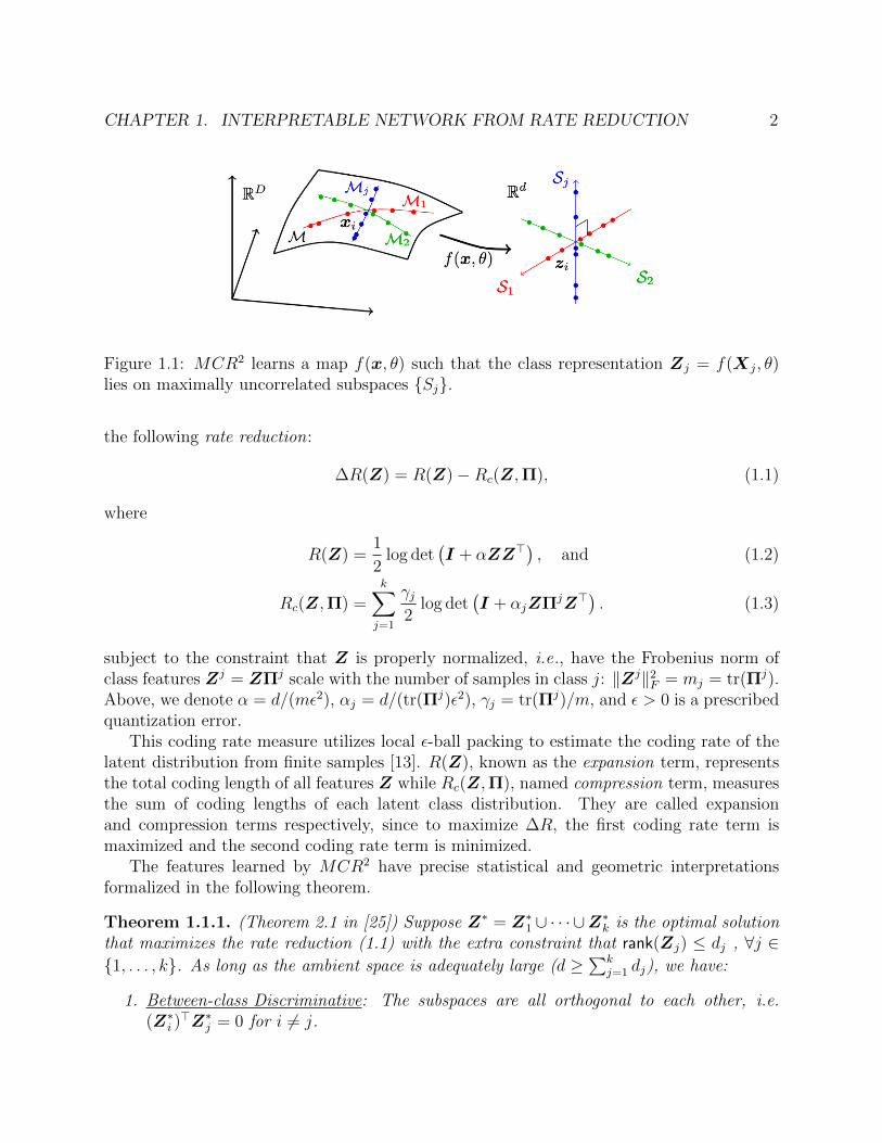
Figure 1.1: MCR2 learns a map f(x, θ) such that the class representation Zj = f(Xj, θ)lies on maximally uncorrelated subspaces {Sj}.
the following rate reduction:
∆R(Z) = R(Z)−Rc(Z,Π), (1.1)
where
R(Z) =1
2log det
(I + αZZ>
), and (1.2)
Rc(Z,Π) =k∑j=1
γj2
log det(I + αjZΠjZ>
). (1.3)
subject to the constraint that Z is properly normalized, i.e., have the Frobenius norm ofclass features Zj = ZΠj scale with the number of samples in class j: ‖Zj‖2
F = mj = tr(Πj).Above, we denote α = d/(mε2), αj = d/(tr(Πj)ε2), γj = tr(Πj)/m, and ε > 0 is a prescribedquantization error.
This coding rate measure utilizes local ε-ball packing to estimate the coding rate of thelatent distribution from finite samples [13]. R(Z), known as the expansion term, representsthe total coding length of all features Z while Rc(Z,Π), named compression term, measuresthe sum of coding lengths of each latent class distribution. They are called expansionand compression terms respectively, since to maximize ∆R, the first coding rate term ismaximized and the second coding rate term is minimized.
The features learned by MCR2 have precise statistical and geometric interpretationsformalized in the following theorem.
Theorem 1.1.1. (Theorem 2.1 in [25]) Suppose Z∗ = Z∗1 ∪ · · · ∪Z∗k is the optimal solutionthat maximizes the rate reduction (1.1) with the extra constraint that rank(Zj) ≤ dj , ∀j ∈{1, . . . , k}. As long as the ambient space is adequately large (d ≥
∑kj=1 dj), we have:
1. Between-class Discriminative: The subspaces are all orthogonal to each other, i.e.(Z∗i )
>Z∗j = 0 for i 6= j.
CHAPTER 1. INTERPRETABLE NETWORK FROM RATE REDUCTION 3
2. Maximally Diverse Representation: As long as the coding precision is adequately high,
i.e., ε4 < minj
{mjm
d2
d2j
}, each subspace achieves its maximal dimension, i.e. rank(Z∗j) =
dj. In addition, the largest dj − 1 singular values of Z∗j are equal.
In [25], it is demonstrated empirically that maximizing ∆R(Z) enforces each latentclass distribution to be a low-dimensional subspace-like distribution of approximately d
k
dimension with class balance i.e. among all such discriminative representations, it prefersthe one that spans the whole ambient space. The data points are distributed isotropically ineach subspace except for possibly one dimension. In addition, these class distributions areorthogonal to each other (See Figure 1.1). Thus, by maximizing the coding rate difference,the features become between-class discriminative, whilst maintaining intra-class diversity.We refer interested readers to [25] for detailed proofs and empirical results.
1.2 Rate Reduction Network (ReduNet)
While an existing neural network architecture (such as ResNet) can be used for featurelearning with MCR2, a follow-up work [2] showed that a novel architecture can be explicitlyconstructed without back-propagation via emulating the projected gradient ascent schemefor maximizing ∆R(Z). This produces a “white box” network, called ReduNet, which hasprecise statistical and geometric interpretations. We review the construction of ReduNet asfollows.
Let Z be initialized as the training data, i.e., Z0 = X. Then, the projected gradientascent step for optimizing the rate reduction ∆R(Z) in (1.1) is given by
Z`+1 ∝ Z` + η
(∂∆R
∂Z
∣∣∣Z`
)= Z` + η
(E`Z` −
k∑j=1
γjCj`Z
j`
)s.t. ‖Zj
`+1‖2F = tr(Πj) = mj ∀j ∈ {1, .., k},
(1.4)
where we use Zj` = Z`Π
j ∈ Rd×m to denote the feature matrix associated with the j-th classat the `-th iteration, and η > 0 is the learning rate. The matrices E` and Cj
` are obtainedby evaluating the derivative ∂∆R
∂Zat Z`, given by
E` = α(I + αZ`Z
>`
)−1, (1.5)
Cj` = αj
(I + αjZ
j`Z
j>`
)−1
. (1.6)
Observe that E` ∈ Rd×d is applied to all features Z` and it expands the coding lengthof the entire data. Meanwhile, Cj
` ∈ Rd×d is applied to features from class j, i.e., Zj`, and it
compresses the coding lengths of the j-th class.
CHAPTER 1. INTERPRETABLE NETWORK FROM RATE REDUCTION 4
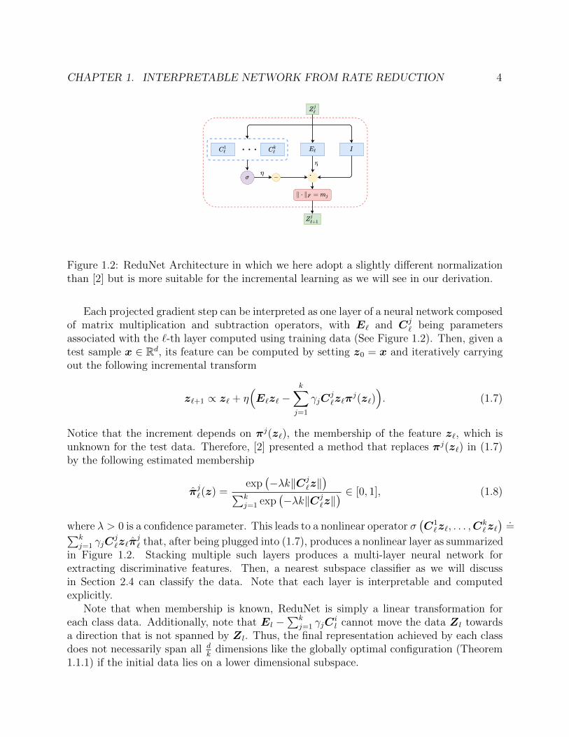
Figure 1.2: ReduNet Architecture in which we here adopt a slightly different normalizationthan [2] but is more suitable for the incremental learning as we will see in our derivation.
Each projected gradient step can be interpreted as one layer of a neural network composedof matrix multiplication and subtraction operators, with E` and Cj
` being parametersassociated with the `-th layer computed using training data (See Figure 1.2). Then, given atest sample x ∈ Rd, its feature can be computed by setting z0 = x and iteratively carryingout the following incremental transform
z`+1 ∝ z` + η(E`z` −
k∑j=1
γjCj`z`π
j(z`)). (1.7)
Notice that the increment depends on πj(z`), the membership of the feature z`, which isunknown for the test data. Therefore, [2] presented a method that replaces πj(z`) in (1.7)by the following estimated membership
π̂j`(z) =exp
(−λk‖Cj
`z‖)∑k
j=1 exp(−λk‖Cj
`z‖) ∈ [0, 1], (1.8)
where λ > 0 is a confidence parameter. This leads to a nonlinear operator σ(C1`z`, . . . ,C
k`z`) .
=∑kj=1 γjC
j`z`π̂
j` that, after being plugged into (1.7), produces a nonlinear layer as summarized
in Figure 1.2. Stacking multiple such layers produces a multi-layer neural network forextracting discriminative features. Then, a nearest subspace classifier as we will discussin Section 2.4 can classify the data. Note that each layer is interpretable and computedexplicitly.
Note that when membership is known, ReduNet is simply a linear transformation foreach class data. Additionally, note that El −
∑kj=1 γjC
il cannot move the data Z l towards
a direction that is not spanned by Z l. Thus, the final representation achieved by each classdoes not necessarily span all d
kdimensions like the globally optimal configuration (Theorem
1.1.1) if the initial data lies on a lower dimensional subspace.
5
Chapter 2
ReduNet for InterpretableIncremental Learning
The work in this chapter was published at the Conference on Computer Vision and PatternRecognition (CVPR) 2021 by the author, Ziyang Wu, Chong You, and Yi Ma [23].
2.1 Introduction
Humans are capable of acquiring new information continuously while retaining previouslyobtained knowledge. This seemingly natural capability, however, is extremely difficult fordeep neural networks (DNNs) to achieve. Incremental learning (IL), also known as continuallearning or life-long learning, thus studies the design of machine learning systems that canassimilate new information without forgetting past knowledge.
In incremental learning, models go through rounds of training sessions to accumulateknowledge for a particular objective (e.g . classification). Specifically, under class incrementallearning (class-IL), an agent has access to training data from a subset of the classes, knownas a task, at each training session and is evaluated on all seen classes at inference time.The overarching goal is to precisely fine-tune a model trained on previously seen tasks toadditionally classify new classes of data. However, due to the absence of old data, such modelsoften suffer from catastrophic forgetting [14], which refers to a drastic drop in performanceafter training incrementally on different tasks.
In the last few years, a flurry of continual learning algorithms have been proposed forDNNs, aiming to alleviate the effect of catastrophic forgetting. These methods can beroughly partitioned into three categories: 1) regularization-based methods that often involveknowledge distillation [12, 6, 19, 26], 2) exemplar-based methods that keep partial copies ofdata from previously learned tasks [16, 1, 22], and 3) modified architectures that attemptto utilize network components specialized for different tasks [17, 19, 11]. In practice, thesealgorithms exhibit varying performance across different datasets and their ability to mitigatecatastrophic forgetting is inadequate. Factors including domain shift [18] across tasks and
CHAPTER 2. REDUNET FOR INTERPRETABLE INCREMENTAL LEARNING 6
imbalance of new and past classes [22] are part of the reason.The fundamental roadblock in deep continual learning is that DNNs are trained and
optimized in a “black box” fashion. Each model contains millions of mathematical operationsand its complexity prevents humans from following the mapping from data input to prediction.Given our current limited understanding of network parameters, it is difficult, if not impossible,to precisely control the parameters of a pre-trained model such that the decision boundarylearned fits to new data without losing its understanding of old data.
In this work, we take a drastically different approach to incremental learning. We avoid“black box” architectures entirely, and instead utilize a recently proposed “white box” DNNarchitecture derived from the principle of rate reduction [2]. Termed ReduNet, each layer ofthis DNN can be explicitly computed in a forward-propagation fashion and each parameterhas precise statistical interpretations. The so-constructed network is intrinsically suitablefor incremental learning because the second-order statistics of any previously-seen trainingdata is preserved in the network parameters to be leveraged for future tasks.
We propose a new incremental learning algorithm utilizing ReduNet to demonstratethe power and scalability of designing more interpretable networks for continual learning.Specifically, we prove that a ReduNet trained incrementally can be constructed to be equivalentto one obtained by joint training, where all data, both new and old, is assumed to be availableat training time. Finally, we observe that ReduNet performs significantly better on MNIST[9] and CIFAR-10 [7] in comparison to current continual DNN approaches.
2.2 Related Work
Since the early success of deep learning in classification tasks such as object recognition,attention has lately shifted to the problem of incremental learning in hopes of designing deeplearning systems that are capable of continuously adapting to data from non-stationary andchanging distributions.
Incremental learning can refer to different problem settings and most studies focus onthree widely accepted scenarios [20]. Most of the earlier works [12, 17, 6, 19] study thetask incremental (task-IL) setting, where a model, after trained on multiple tasks, must beable to classify on data belonging to all the classes it has seen so far. However, the model isadditionally provided a task-ID indicating the task or subset of classes each datapoint belongsto. Models trained under this setting are thus required to distinguish among typically onlya small number of classes. Recent works [24, 27] explore the more difficult class incremental(class-IL) setting, where task-ID is withheld at inference time. This setting is considerablymore difficult since without the task-ID, each datapoint could potentially belong to any ofthe classes the model has seen so far. The other setting, known as domain incrementallearning (domain-IL) differs from the previous two settings in that each task consists of allthe classes the model needs to learn. Instead, a task-dependent transformation is applied tothe data. For example, each task could contain the same training data rotated by differing
CHAPTER 2. REDUNET FOR INTERPRETABLE INCREMENTAL LEARNING 7
degrees and the model must learn to classify images of all possible rotations without accessto the task-ID.
Deep continual learning literature from the last few years can be roughly partitioned intothree categories as follows:
Regularization-based methods usually attempt to preserve some part of the networkparameters deemed important for previously learned tasks. Knowledge distillation [4] is apopular technique utilized to preserve knowledge obtained in the past. Learning withoutForgetting (LwF) [12], for example, attempts to prevent the model parameters from largedrifts during the training of the current task by employing cross-entropy loss regularized bya distillation loss. Alternatively, elastic weight consolidation (EWC) [6] attempts to curtaillearning on weights based on their importance to previously seen tasks. This is done byimposing a quadratic penalty term that encourages weights to move along directions withlow Fisher information. Schwarz et al . [19] later proposed an online variant (oEWC) thatreduces the cost of estimating the Fisher information matrix. Similarly, Zenke et al . [26]limits the changes of important parameters in the network by using an easy-to-computesurrogate loss during training.
Exemplar-based methods typically use a memory buffer to store a small set of datafrom previous tasks in order to alleviate catastrophic forgetting. The data stored is usedalong with the data from the current task to jointly train the model. Rebuffi et al . [16]proposed iCaRL which uses a herding algorithm to decide which samples from each class tostore during each training session. This technique is combined with regularization with adistillation loss to further encourage knowledge retention [16]. A recent work by Wu et al .[22] achieved further improvements by correcting the bias towards new classes due to dataimbalance, which they empirically show causes degradation in performance for large-scaleincremental learning settings. This is accomplished by appending a bias-correction layerat the end of the network. Another increasingly popular approach is to train a generativeadversarial network (GAN) [5, 21] on previously seen classes and use the generated syntheticdata to facilitate training on future tasks.
Architecture-based methods either involve designing specific components in the architectureto retain knowledge of previously seen data or appending new parameters or entire networkswhen encountering new classes of data. Progressive Neural Network (PNN) [17], for example,instantiates a new network for each task with lateral connection between networks in orderto overcome forgetting. This results in the number of networks to grow linearly with respectto the number of tasks as training progresses. Progress & Compress (P & C) [19] utilizes onenetwork component to learn the new task, then distills knowledge into a main componentthat aggregates knowledge from previously encountered data. Li et al . [11], proposes a neuralarchitecture search method that utilizes a separate network to learn whether to reuse, adapt,or add certain building blocks of the main classification network for each task encountered.
Our work studies the more difficult class-IL scenario and does not involve regularizationor storing any exemplars. Our method thus can be characterized as an architecture-basedapproach. However, our method differs with the aforementioned works in several importantaspects. First, we use a “white box” architecture that is computed exactly in a feed-forward
CHAPTER 2. REDUNET FOR INTERPRETABLE INCREMENTAL LEARNING 8
manner. Moreover, the network, when trained under class-IL scenario, can be shown toperform equivalently to one obtained from joint training while most existing works [11, 19,17] based on modified architectures target the less challenging task-IL setting. We discussthe differences in more detail later in Section 2.3, after we have introduced our methodproperly.
2.3 Incremental Learning with ReduNet
In this paper, we tackle the task of class incremental learning, formalized as follows. Supposewe have a stream of tasks D1,D2, . . . ,Dt, . . ., where each task Dt consists of data from ktclasses, i.e, Dt = {X(t−1)·kt+1, . . . ,X t·kt} where Xj is a set of points in class j. The classesin different tasks are assumed to be mutually exclusive. Furthermore, it is assumed thatthe tasks arrive in an online setting, meaning that at timestep t when data Dt arrives, thedata associated with old tasks {Di, i < t} becomes unavailable. Therefore, the objective isto design a learning system that can adapt the model from the old tasks so as to correctlyclassify on all tasks hitherto, i.e., D1, . . . ,Dt. In addition, we assume that we are not giventhe information on the task a test data belongs to, making this problem significantly morechallenging than task-IL.
In this section, we show that ReduNet can perfectly adapt to a new task withoutforgetting old tasks. Specifically, we present an algorithm to adapt the ReduNet constructedfrom data {Di, i < t} by using only the data in Dt, so that the updated ReduNet is exactlythe same as the ReduNet constructed as if data from all tasks {Di, i ≤ t} were available.
Derivation of Incrementally-Trained ReduNet
Without loss of generality, we consider the simple case with two tasks t and t′ where t istreated as the old task and t′ is treated as the new task. Assume that t and t′ contain mt,mt′ training samples and kt, kt′ distinct classes, respectively. We denote such training databy Z0,t ∈ Rd×mt (for task t) and Z0,t′ ∈ Rd×mt′ (for task t′), and assume that they havebeen normalized by Frobenius norm as described in (1.4). For ease of notation, we label theclasses as {1, ..., kt} for task t and {kt + 1, ..., kt + kt′} for task t′.
Let Θt be the ReduNet of depth L trained on task t as described in Section 1.2. Giventhe new task Z0,t′ , our objective is to train a network Θt→t′ that adapts Θt to have goodperformance for both tasks t and t′. Next, we show that a network Θt→t′ can be constructedfrom Θt andZ0,t′ such that it is equivalent to Θ obtained from training onZ0 = [Z0,t|Z0,t′ ] ∈Rd×m where m = mt +mt′ .
To start, consider the initial expansion term E0 ∈ Rd×d and compression terms Cj0 at
layer 0 of the joint network Θ given by
E0 = α(I + αZ0Z
>0
)−1
= α(I + α
(Z0,tZ
>0,t +Z0,t′Z
>0,t′
))−1,
(2.1)
CHAPTER 2. REDUNET FOR INTERPRETABLE INCREMENTAL LEARNING 9
and
Cj0 =
αj(I + αjZ
j0,tZ
j>0,t
)−1
, if j ≤ kt,
αj
(I + αjZ
j0,t′Z
j>0,t′
)−1
, else(2.2)
where α = d/(mε2) and αj = d/(tr(Πj)ε2).
Note that the term Zj0,t′Z
j>0,t′ can be directly computed from input data Zj
0,t′ . On the
other hand, the term Zj0,tZ
j>0,t cannot be directly computed from input data as Zj
0,t is fromthe old task, which is no longer available under the IL setup. Our key observation is thatZj
0,tZj>0,t can be computed from the network Θt. Specifically, by denoting the compression
matrices of Θt as {Cj`,t} for ` ∈ {0, ..., L− 1}, we have
Zj0,tZ
j>0,t =
((Cj
0,t/αj)−1 − I
)/αj. (2.3)
Next, we show by induction that one can recursively compute E` and {Cj`} of Θ for
` > 0 from (2.1) and (2.2). To construct layer 1 of Θ, we observe that the output featuresof class j at layer 0 before normalization is as follows.
P j0 = (Z0 + ηE0Z0 − η
k∑i=1
γiCi0Z
i0)Πj (2.4)
= Zj0 + ηE0Z
j0 − ηγjC
j0Z
j0 (2.5)
=(I + ηE0 − ηγjCj
0︸ ︷︷ ︸Lj0∈Rd×d
)Zj
0. (2.6)
Notice the term Lj0 only depends on quantities already obtained at layer 0. To compute E1
and Cj1, we need the covariance matrix of P j
0, which we observe to be
T j1 = P j
0Pj>0 = Lj0Z
j0Z
j>0 L
j>0 . (2.7)
Notice that T j1 can be expressed with known quantities of Lj0 and Zj
0,tZj>0,t if j ≤ kt or
Zj0,t′Z
j>0,t′ if j > kt. The remaining step would be to re-scale T j
1 as the updated representation
P j0 needs to be normalized to get Zj
1. Recall that we adopt the normalization scheme thatimposes the Frobenius norm of each class Zj to scale with mj:
‖Zj1‖2F = mj ⇐⇒ tr
(Zj
1Zj1
>)= mj. (2.8)
The re-scaling factor is then easy to calculate:
Zj1Z
j>1 =
mj
tr(T j1)T j
1. (2.9)
CHAPTER 2. REDUNET FOR INTERPRETABLE INCREMENTAL LEARNING 10
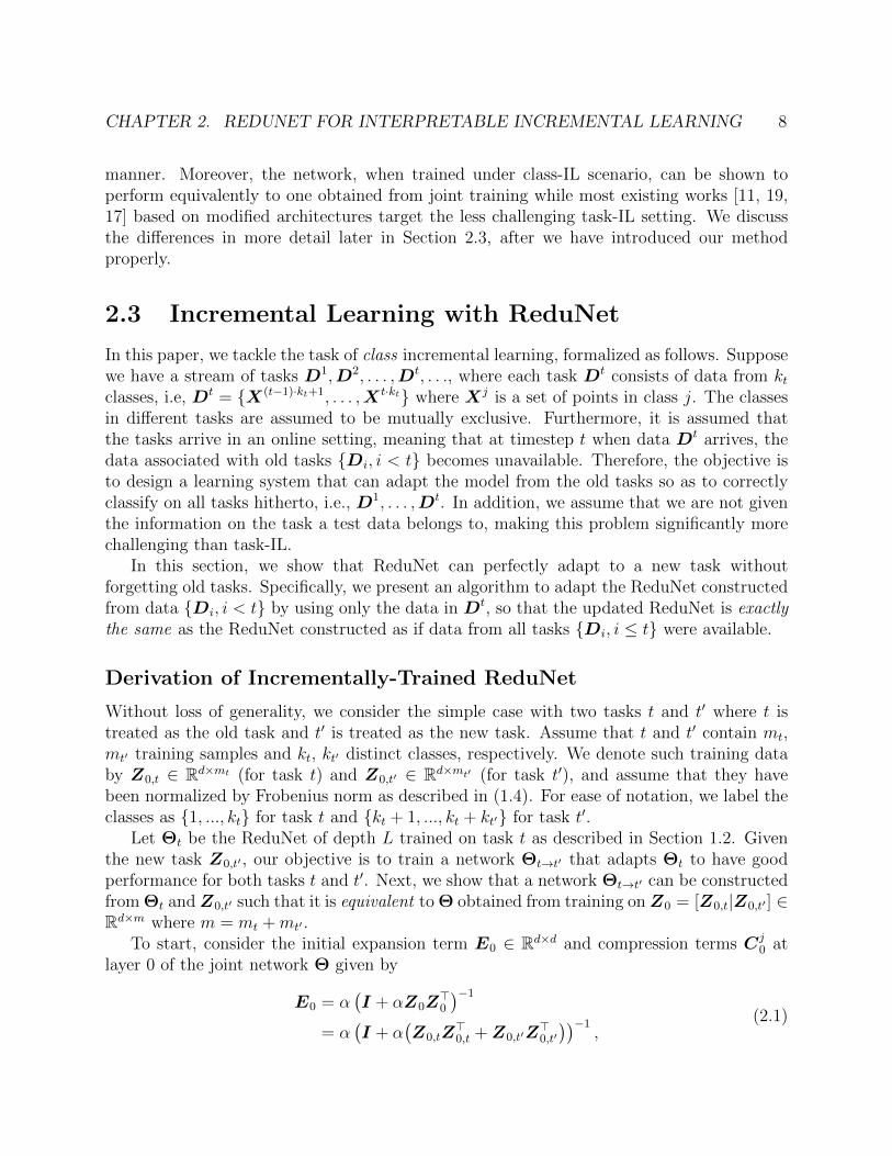
Figure 2.1: The joint network can be derived using simply Z0,tZ>0,t. We do not need the
task t data Z0,t directly.
From above, we see that we can obtain the correct value of the covariance matrix Zj1Z
j>1 ,
from which we can derive E1 and Cj1 for layer 1 of the joint network Θ and obtain Zj
2,t′ .
With these values, we can compute T j2.
By the same logic, we can recursively updateE` andCj` for all ` > 1. Specifically, once we
have obtained Zj`−1Z
j>`−1 and Lj`−1, it is straightforward to compute T j
` = L`−1Zj`−1Z
j>`−1L
j>`−1
and therefore obtain
Zj`Z
j>` =
mj
tr(T j`)T j`. (2.10)
Note that we never need to access Z0,t ∈ Rd×mt directly. Instead, we iteratively update the
covariance matrix Zj`−1,tZ
j>`−1,t ∈ Rd×d for each class j using the procedure described. This
concludes our induction and Algorithm 1 describes the entire training process for incrementallearning on two tasks. The procedure is illustrated in Figure 2.1. This procedure can benaturally extended to settings with more than two tasks.
Comparison to Existing Methods
Incremental learning with ReduNet offers several nice properties: 1) Each parameter of thenetwork has an explicit purpose, computed precisely to emulate the gradient ascent on thefeature representation. 2) It does not require a memory buffer which is often needed inmany state-of-the-art methods [16, 22, 1]. 3) It can be proven to behave like a networkreconstructed from joint training, thus eliminating the problem of catastrophic forgetting.
Note that many existing works without relying on exemplars [12, 6, 19, 26] regularize theoriginal weights of the model at each training session, effectively freezing certain parts of the
CHAPTER 2. REDUNET FOR INTERPRETABLE INCREMENTAL LEARNING 11
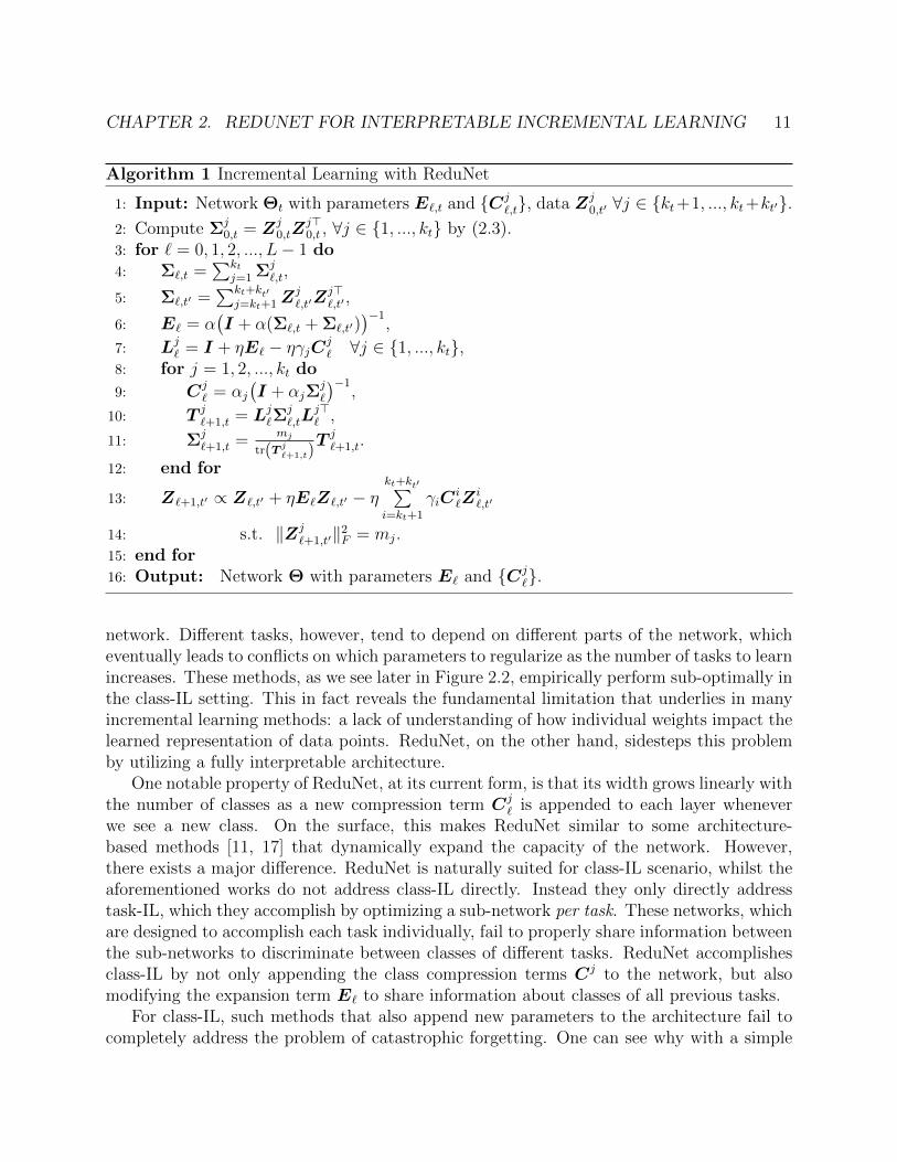
Algorithm 1 Incremental Learning with ReduNet
1: Input: Network Θt with parameters E`,t and {Cj`,t}, data Zj
0,t′ ∀j ∈ {kt+1, ..., kt+kt′}.2: Compute Σj
0,t = Zj0,tZ
j>0,t , ∀j ∈ {1, ..., kt} by (2.3).
3: for ` = 0, 1, 2, ..., L− 1 do4: Σ`,t =
∑ktj=1 Σj
`,t,
5: Σ`,t′ =∑kt+kt′
j=kt+1Zj`,t′Z
j>`,t′ ,
6: E` = α(I + α(Σ`,t + Σ`,t′)
)−1,
7: Lj` = I + ηE` − ηγjCj` ∀j ∈ {1, ..., kt},
8: for j = 1, 2, ..., kt do
9: Cj` = αj
(I + αjΣ
j`
)−1,
10: T j`+1,t = Lj`Σ
j`,tL
j>` ,
11: Σj`+1,t =
mj
tr(T j`+1,t)T j`+1,t.
12: end for
13: Z`+1,t′ ∝ Z`,t′ + ηE`Z`,t′ − ηkt+kt′∑i=kt+1
γiCi`Z
i`,t′
14: s.t. ‖Zj`+1,t′‖2
F = mj.15: end for16: Output: Network Θ with parameters E` and {Cj
`}.
network. Different tasks, however, tend to depend on different parts of the network, whicheventually leads to conflicts on which parameters to regularize as the number of tasks to learnincreases. These methods, as we see later in Figure 2.2, empirically perform sub-optimally inthe class-IL setting. This in fact reveals the fundamental limitation that underlies in manyincremental learning methods: a lack of understanding of how individual weights impact thelearned representation of data points. ReduNet, on the other hand, sidesteps this problemby utilizing a fully interpretable architecture.
One notable property of ReduNet, at its current form, is that its width grows linearly withthe number of classes as a new compression term Cj
` is appended to each layer wheneverwe see a new class. On the surface, this makes ReduNet similar to some architecture-based methods [11, 17] that dynamically expand the capacity of the network. However,there exists a major difference. ReduNet is naturally suited for class-IL scenario, whilst theaforementioned works do not address class-IL directly. Instead they only directly addresstask-IL, which they accomplish by optimizing a sub-network per task. These networks, whichare designed to accomplish each task individually, fail to properly share information betweenthe sub-networks to discriminate between classes of different tasks. ReduNet accomplishesclass-IL by not only appending the class compression terms Cj to the network, but alsomodifying the expansion term E` to share information about classes of all previous tasks.
For class-IL, such methods that also append new parameters to the architecture fail tocompletely address the problem of catastrophic forgetting. One can see why with a simple
CHAPTER 2. REDUNET FOR INTERPRETABLE INCREMENTAL LEARNING 12
example. Consider an ensemble learning technique where for each class j, we train an all-versus-one model that predicts whether a data point belongs to class j or not. At each task,we can feed the available data points into each model, labeled as 1 if it belongs in thatclass or 0 otherwise. However, by optimizing such “black box” models by back-propagation,we again arrive at the problem of catastrophic forgetting. Specifically, the model only seestraining points of its own class only for one task or training session. For the remaining tasks,all data points that it must train will be of label 0, which prevents standard gradient descentfrom correctly learning the desired all-versus-one decision boundary, and there is no clearway to precisely address this optimization problem.
Although it is natural to expect the network to expand as the number of classes increases,it remains interesting to see if the growth of certain variations of the ReduNet can besublinear instead of linear in the number of classes.
2.4 Experiments
We evaluate the proposed method on MNIST and CIFAR-10 datasets in a class-IL scenarioand compare the results with existing methods. In short, for both MNIST and CIFAR-10,the 10 classes are split into 5 incremental batches or tasks of 2 classes each. After trainingon each task, we evaluate the model’s performance on test data from all classes the modelhas seen so far. The same setting is applied to all other methods we compared to.
Datasets
We compare the incremental learning performance of ReduNet on the following two standarddatasets.MNIST [10]. MNIST contains 70,000 greyscale images of handwritten digits 0-9, whereeach image is of size 28 × 28. The dataset is split into training and testing sets, where thetraining set contains 60,000 images and the testing dataset contains 10,000 images.CIFAR-10 [8]. CIFAR-10 contains 60,000 RGB images of 10 object classes, where eachimage is of size 32 × 32. Each class has 5,000 training images and 1,000 testing images.We normalize the input data by dividing the pixel values by 255, and subtracting the meanimage of the training set.
Implementation Details
We implement ReduNet for each training dataset in the following manner.ReduNet on MNIST. To construct a ReduNet on MNIST, we first flatten the input imageand represent it by a vector of dimension 784. Then, with a precision ε = 0.5 in the MCR2
objective (1.1), we apply 200 iterations of projected gradient iterations to compute E` andCj` matrices for each iteration `. The learning rate is set to η = 0.5 × 0.933` at the `-th
iteration. These matrices are the parameters of the constructed ReduNet. Given a test
CHAPTER 2. REDUNET FOR INTERPRETABLE INCREMENTAL LEARNING 13
data, its feature can be extracted with the incremental transform in (1.7) with estimatedlabels computed as in (1.8) with parameter λ = 1. At each training session, we update theReduNet by the procedure described in Algorithm 1.
We note that hyper-parameter tuning in ReduNet does not require a training/validationsplitting as in regular supervised learning methods. The hyper-parameters described abovefor ReduNet are chosen based on the training data. This is achieved by evaluating theestimated label through (1.8) on the training data, and comparing such labels with groundtruth labels. Then, the model parameter ε, learning rate η and the softmax confidenceparameter λ are chosen as those that gives the highest accuracy with the estimated labels(at the final layer).ReduNet on CIFAR-10. We apply 5 random Gaussian kernels with stride 1, size 3×3 onthe input RGB images.1 This lifts each image to a multi-channel signal of size 32× 32× 5,which is subsequently flattened to be a R5,120 dimensional vector. Subsequently, we constructa 50-layer ReduNet with all other hyper-parameters the same as those for MNIST. Allhyperparameters stated above, including the depth of the network, were chosen such thatthe ∆R loss has sufficiently converged.Comparing Methods. We compare our approach to the following state of the art algorithms:iCaRL [16], LwF [12], oEWC [19], SI [26] and DER [1]. For these algorithms, we utilize thesame benchmark and training protocol as Buzzega et al . [1]. For MNIST, we employ a fully-connected network with two hidden layers comprised of 100 ReLU units. For CIFAR-10,we rely on ResNet18 without pre-training [3]. All the networks were trained by stochasticgradient descent. For MNIST, we train on one epoch per task. For CIFAR-10, we trainon 100 epochs per task. The number of epochs were chosen based on the complexity ofthe dataset. For each algorithm, batch size, learning rate, and specific hyperparameters foreach algorithm were selected by performing a grid-search using 10% of the training data asa validation set and selecting the hyperparameter that achieves the highest final accuracy.The optimal hyperparameters utilized for the benchmark experiments are reported in [1].
The performance of state of the art algorithms utilizing a replay buffer highly dependson the number of exemplars, or samples from previous tasks, it is allowed to retain. We teston two exemplar-based algorithm, iCaRL and DER. For both MNIST and CIFAR-10, we setthe total number of exemplars to 200.
Nearest Subspace Classification
By the principle of maximal rate reduction, the ReduNet f(X, θ) extracts features such thateach class lies in a low-dimensional linear subspace and different subspaces are orthogonal.As suggested by the original MCR2 work [2], we utilize a nearest subspace classifier to classifythe test data featurized to maximize ∆R. Given a test sample ztest = f(xtest, θ), the label
1This choice is limited by our current computational resources. Although this choice is not adequateto achieve top classification performance, it is adequate to verify the advantages of our method in theincremental setting.
CHAPTER 2. REDUNET FOR INTERPRETABLE INCREMENTAL LEARNING 14
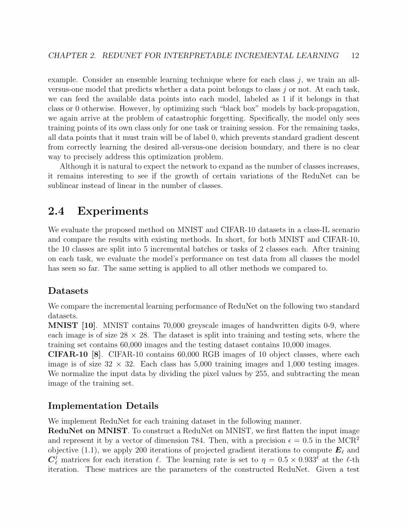
Algorithm MNIST CIFAR-10Task 1 Task 2 Task 3 Task 4 Task 5 Task 1 Task 2 Task 3 Task 4 Task 5
LwF 0.999 0.009 0.0 0.0 0.0 0.979 0.0 0.0 0.0 0.0oEWC 1.0 0.004 0.0 0.0 0.0 0.981 0.0 0.0 0.0 0.0
SI 0.997 0.004 0.001 0.0 0.0 0.989 0.0 0.0 0.0 0.0iCaRL (200 Exemplars) 0.999 0.806 0.708 0.612 0.596 0.964 0.720 0.427 0.362 0.313DER (200 Exemplars) 0.999 0.967 0.941 0.883 0.735 0.985 0.816 0.608 0.404 0.292
ReduNet(Ours) 0.999 0.994 0.993 0.989 0.987 0.875 0.754 0.714 0.642 0.562Upper Bound (UB) 0.999 0.995 0.990 0.988 0.982 0.989 0.971 0.957 0.963 0.920
Table 2.1: Test Accuracy (%) on Task 1 After Each Training Session on MNIST and CIFAR-10.
predicted by a nearest subspace classifier is
y = arg miny∈1,...,k
∥∥(I −U yU y>)ztest∥∥2
2, (2.11)
where U y is a matrix containing the top x principal components of the covariance of thetraining data passed through ReduNet, i.e. ZtrainZ
>train for Ztrain = f(X train, θ).
Since we do not have access toZtrain during evaluation, we instead collect theCj matricesat the very last layer L and extract the covariance matrix Σj
L to be further processed bySVD. For MNIST, we utilize the top 28 principal components. For CIFAR-10, we utilize thetop 15 principal components.
Results and Analysis
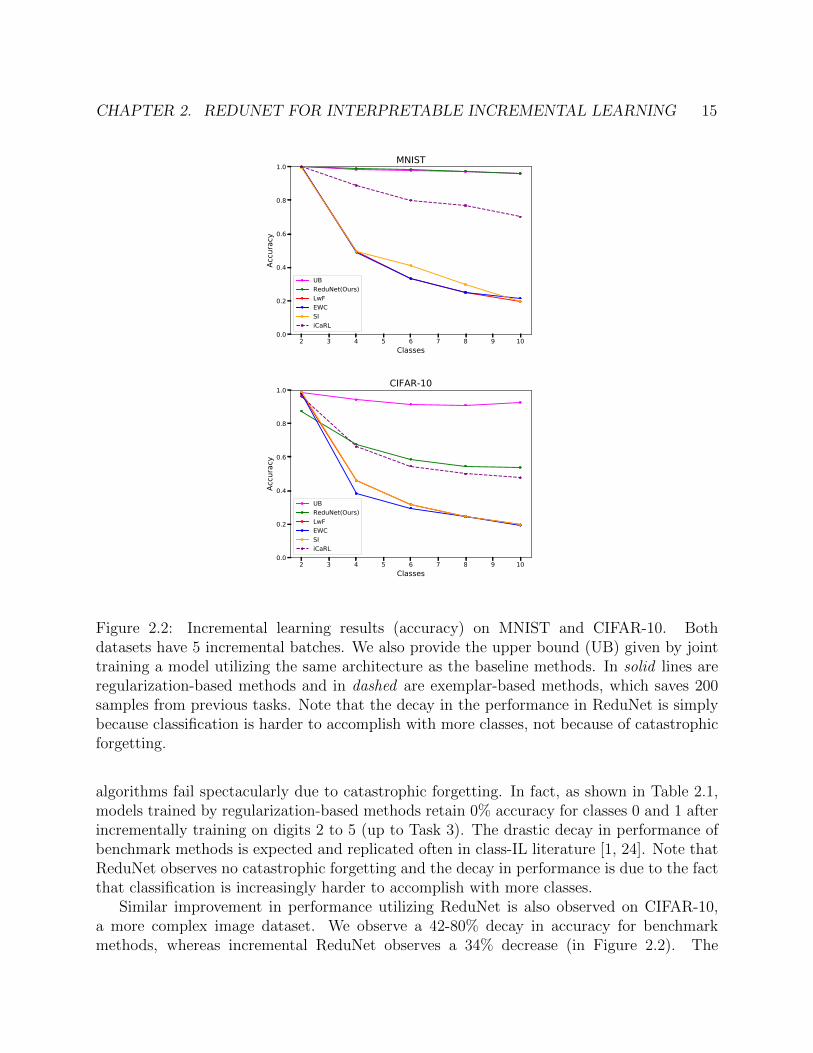
In this section, we evaluate the class-IL performance of incremental ReduNet against threeregularization-based methods (oEWC, SI, LwF) and two replay-based methods leveraging200 exemplars (iCaRL, DER) on MNIST and CIFAR-10. We also provide the upper bound(UB) achieved by joint training a model utilizing the same architecture as the baselinemethods. After the model is trained on each task, performance is evaluated by computingthe accuracy on test data from all classes the model has seen so far. To observe the degree offorgetting, we record the model’s performance on Task 1 after training on each subsequenttask. For both MNIST and CIFAR-10, we observe a substantial performance increase byutilizing incremental ReduNet as shown in Figure 2.2. Additionally, we observe ReduNetshows significantly less forgetting (see Table 2.1).
On MNIST, we observe a 3% decay in accuracy across the tasks on ReduNet versus a20-80% decay on benchmark methods (Figure 2.2). We measure decay as the difference inaverage accuracy between the first and last task. ReduNet retains a classification accuracyof 96%. This is of no surprise since MNIST is relatively linearly separable, allowing second-order information about the data to be sufficient for ReduNet to correctly classify thedigits. We observe that even for a very simple task as MNIST, competing continual learning
CHAPTER 2. REDUNET FOR INTERPRETABLE INCREMENTAL LEARNING 15
2 3 4 5 6 7 8 9 10Classes
0.0
0.2
0.4
0.6
0.8
1.0
Accu
racy
MNIST
UBReduNet(Ours)LwFEWCSIiCaRL
2 3 4 5 6 7 8 9 10Classes
0.0
0.2
0.4
0.6
0.8
1.0
Accu
racy
CIFAR-10
UBReduNet(Ours)LwFEWCSIiCaRL
Figure 2.2: Incremental learning results (accuracy) on MNIST and CIFAR-10. Bothdatasets have 5 incremental batches. We also provide the upper bound (UB) given by jointtraining a model utilizing the same architecture as the baseline methods. In solid lines areregularization-based methods and in dashed are exemplar-based methods, which saves 200samples from previous tasks. Note that the decay in the performance in ReduNet is simplybecause classification is harder to accomplish with more classes, not because of catastrophicforgetting.
algorithms fail spectacularly due to catastrophic forgetting. In fact, as shown in Table 2.1,models trained by regularization-based methods retain 0% accuracy for classes 0 and 1 afterincrementally training on digits 2 to 5 (up to Task 3). The drastic decay in performance ofbenchmark methods is expected and replicated often in class-IL literature [1, 24]. Note thatReduNet observes no catastrophic forgetting and the decay in performance is due to the factthat classification is increasingly harder to accomplish with more classes.
Similar improvement in performance utilizing ReduNet is also observed on CIFAR-10,a more complex image dataset. We observe a 42-80% decay in accuracy for benchmarkmethods, whereas incremental ReduNet observes a 34% decrease (in Figure 2.2). The
CHAPTER 2. REDUNET FOR INTERPRETABLE INCREMENTAL LEARNING 16
algorithm that achieves the closest performance to ReduNet is iCaRL and DER, exemplar-based methods that require access to 200 previously observed exemplars. Certainly, as canbe seen by the 88% accuracy on Task 1 of CIFAR-10, ReduNet at its current basic form (onlyusing 5 randomly initialized kernels without back-propagation) is not able to reach the sameclassification accuracy as ResNet-18 for complex image classification tasks. It is thus notsurprising that DER, based on more established network architectures, exceeds ReduNet interms of average accuracy. However, as shown in Table 2.1, ReduNet decays gracefully andsignificantly outperforms other methods in terms of forgetting, retaining over 55% accuracyon Task 1 versus less than 30% by DER.
We note that ReduNet is currently a slower training framework given its current naiveimplementation using CuPy. Utilizing a single NVIDIA TITAN V GPU, each task trainingsession took approximately 1500 seconds for MNIST and 9200 seconds for CIFAR10. Onthe other hand, joint training a model by back-propagation for each task took 23 and 2500seconds for MNIST and CIFAR10, respectively.
2.5 Conclusions and Future Work
We demonstrated through an incremental version of the recently proposed ReduNet, thepromise of leveraging interpretable network design for continual learning. The proposednetwork has shown significant performance increases in both synthetic and complex realdata, even without utilizing any fine-tuning with back-propagation. It has clearly shownthat if knowledge of past learned tasks are properly utilized, catastrophic forgetting needsnot to happen as new tasks continue to be learned.
We purpose of this work is not to push the state of art classification accuracy or efficiencyon any single large-scale real-world dataset. Rather we want to use the simplest experimentsto show beyond doubt the remarkable effectiveness and great potential of this new framework.Using CIFAR-10 as an example, simply utilizing a relatively small set of 5 random liftingkernels was already sufficient for a decent incremental classification performance. We believethat to achieve better performance for more complex tasks and datasets, judicious design orlearning of more convolution kernels would be needed. This leaves plenty of room for furtherimprovements.
This work also opens up a few promising new extensions. As we have mentioned earlier,the current framework requires the width of the network to grow linearly in the number ofclasses. It would be interesting to see if some of the filters can be shared among old/newclasses so that the growth can be sublinear. In the next chapter, we will discuss severalapproaches to decrease the memory footprint of incremental ReduNet.
To a large extent, the rate reduction gives a unified measure for learning discriminativerepresentations in supervised, semi-supervised, and unsupervised settings. We believe ourmethod can be easily extended to cases when some of the new data do not have classinformation.
17
Chapter 3
Low Rank Approximation for EfficientReduNet
As we’ve observed in the previous chapter, incremental ReduNet tends to have a largememory footprint that increases linearly in the number of classes k. Namely, given ddimensional data, each layer requires one to save k + 1 d × d weight matrices: El,t, {Cj
l,t}.In this chapter, we discuss naive, yet effective methods at reducing this memory footprint.
3.1 Low rank approximation
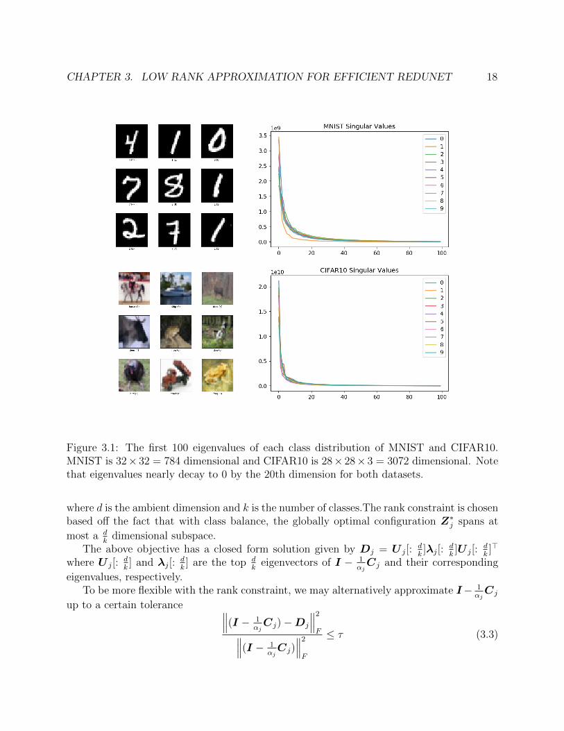
Though real world data such as images are often high dimensional, we often expect the datafrom each class to lie on low dimensional curved manifolds. For example, for MNIST andCIFAR-10, the singular values of the sample covariance matrix of each class is very smallacross most dimensions (Figure 3.1). Thus, the matrices are approximately low-rank.
We may utilize this understanding to find a substantially compressed version of ReduNetwith equal performance. Namely, note that given that the distribution of class j, ZjZ
>j , is
low rank, I − 1αjCj is also low rank where Cj is the corresponding compression matrix.
1
αjCj = (I + cjZjZ
>j )−1 = Ujdiag
(1
1 + cjλji
)Uj>
⇒ I − 1
αjCj = Ujdiag
(1− 1
1 + cjλji
)Uj>
(3.1)
We may find a low rank approximation of the compression matrix by optimizing over thefollowing objective.
minDj
∥∥∥∥(I − 1
αjCj)−Dj
∥∥∥∥2
F
subject to rank(Dj) <d
k
(3.2)
CHAPTER 3. LOW RANK APPROXIMATION FOR EFFICIENT REDUNET 18
Figure 3.1: The first 100 eigenvalues of each class distribution of MNIST and CIFAR10.MNIST is 32× 32 = 784 dimensional and CIFAR10 is 28× 28× 3 = 3072 dimensional. Notethat eigenvalues nearly decay to 0 by the 20th dimension for both datasets.
where d is the ambient dimension and k is the number of classes.The rank constraint is chosenbased off the fact that with class balance, the globally optimal configuration Z∗j spans at
most a dk
dimensional subspace.The above objective has a closed form solution given by Dj = U j[:
dk]λj[:
dk]U j[:
dk]>
where U j[:dk] and λj[:
dk] are the top d
keigenvectors of I − 1
αjCj and their corresponding
eigenvalues, respectively.To be more flexible with the rank constraint, we may alternatively approximate I− 1
αjCj
up to a certain tolerance ∥∥∥(I − 1αjCj)−Dj
∥∥∥2
F∥∥∥(I − 1αjCj)
∥∥∥2
F
≤ τ (3.3)
CHAPTER 3. LOW RANK APPROXIMATION FOR EFFICIENT REDUNET 19
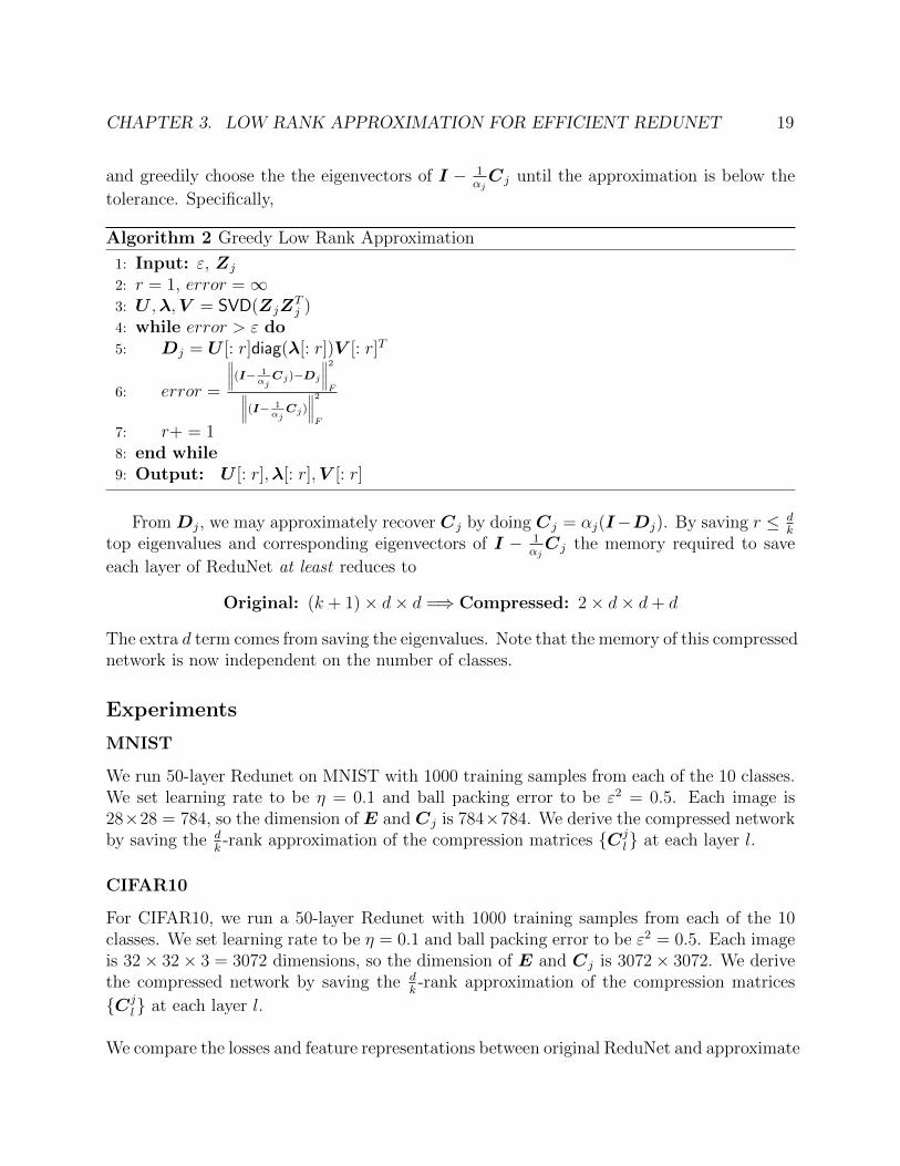
and greedily choose the the eigenvectors of I − 1αjCj until the approximation is below the
tolerance. Specifically,
Algorithm 2 Greedy Low Rank Approximation
1: Input: ε, Zj
2: r = 1, error =∞3: U ,λ,V = SVD(ZjZ
Tj )
4: while error > ε do5: Dj = U [: r]diag(λ[: r])V [: r]T
6: error =
∥∥∥∥(I− 1αj
Cj)−Dj
∥∥∥∥2F∥∥∥∥(I− 1
αjCj)
∥∥∥∥2F
7: r+ = 18: end while9: Output: U [: r],λ[: r],V [: r]
From Dj, we may approximately recover Cj by doing Cj = αj(I−Dj). By saving r ≤ dk
top eigenvalues and corresponding eigenvectors of I − 1αjCj the memory required to save
each layer of ReduNet at least reduces to
Original: (k + 1)× d× d =⇒ Compressed: 2× d× d+ d
The extra d term comes from saving the eigenvalues. Note that the memory of this compressednetwork is now independent on the number of classes.
Experiments
MNIST
We run 50-layer Redunet on MNIST with 1000 training samples from each of the 10 classes.We set learning rate to be η = 0.1 and ball packing error to be ε2 = 0.5. Each image is28×28 = 784, so the dimension of E and Cj is 784×784. We derive the compressed networkby saving the d
k-rank approximation of the compression matrices {Cj
l } at each layer l.
CIFAR10
For CIFAR10, we run a 50-layer Redunet with 1000 training samples from each of the 10classes. We set learning rate to be η = 0.1 and ball packing error to be ε2 = 0.5. Each imageis 32× 32× 3 = 3072 dimensions, so the dimension of E and Cj is 3072× 3072. We derivethe compressed network by saving the d
k-rank approximation of the compression matrices
{Cjl } at each layer l.
We compare the losses and feature representations between original ReduNet and approximate
CHAPTER 3. LOW RANK APPROXIMATION FOR EFFICIENT REDUNET 20
0 10 20 30 40 50Layer
100
200
300
400
500
600
R
Approximate RTrue R
(a) MNIST
0 10 20 30 40 50Layer
500
1000
1500
2000
2500
3000
R
Approximate RTrue R
(b) CIFAR10
Figure 3.2: We pass through the training data of MNIST and CIFAR10 through the originalReduNet and compressed ReduNet, and compare the MCR loss ∆R(Z l) at each layer l. Weobserve the loss curve for compressed ReduNet to be better than that of true ReduNet
ReduNet. Recall that the class distributions of MNIST are already quite low rank andseparable (Figure 3.1). Since the class distributions of CIFAR10 and MNIST are lowdimensional, we observe that the low rank approximations of the compression matrices Cj
l
are close to the original matrices. Furthermore, compressed ReduNet achieved better losscurves than true ReduNet. By compressing ReduNet up to some tolerance, we were able toreduce the memory footprint of the network even further 3.3.
3.2 Block Diagonal Approximation by Eigenspace
We may further compress the model from our knowledge that the eigenvectors of eachclass distribution ZjZ
>j must be some linear combination of the eigenvectors of the joint
distribution ZZ> =∑
j ZjZ>j . In fact, at a critical point Z∗ of the loss ∆R, the eigenvectors
of ZZ> is precisely equal to the eigenvectors of ZjZ>j . This statement is formalized in the
following theorem.
Theorem 3.2.1. If Z∗ is a local maxima of ∆R(Z), then each eigenvector with positive
CHAPTER 3. LOW RANK APPROXIMATION FOR EFFICIENT REDUNET 21
0.01 0.04 0.07 0.10 0.13 0.16 0.19 0.22 0.25 0.28 0.31 0.34 0.37 0.40 0.43 0.46 0.49 0.52 0.55 0.58 0.61 0.64 0.67 0.70 0.73 0.76 0.79 0.82 0.85 0.88 0.91 0.94 0.97tolerance
0
3
6
9
12
15
18
21
24
27
30
33
36
39
42
45
48
51
54
57
rr vs tolerance
class 0class 1class 2class 3class 4
Figure 3.3: In MNIST, we observe that only a few eigenvectors are necessary to approximateCj of the first layer for small tolerance values.
corresponding eigenvalue of the class subspace Z∗jZ∗>j must be an eigenvector of the whole
distribution Z∗Z∗>.
Proof. Recall MCR2 objective:
max ∆R(Z) = R(Z, ε)−Rc(Z, ε|Π) s.t. ‖Zj‖2F = mj ∀j ∈ {1, ..., k} (3.4)
By first order necessary conditions, note that Z is a stationary point if for each classdistribution ∇Zj∆R = ajZj for some constant aj ∈ R. Recall that the gradient is
∂∆R
∂Zj
=(E − γjCj
`
)Zj (3.5)
So at a stationary point, each sample zji in Zj for i ∈ 1, ...,mj satisfies
(E − γjCj)zji = ajz
ji .
Furthermore, note that each eigenvector ujl of ZjZ>j for 0 ≤ l ≤ d with corresponding
eigenvalue λjl > 0, is some linear combination of class samples
ujl =
mj∑i=1
αizji .
CHAPTER 3. LOW RANK APPROXIMATION FOR EFFICIENT REDUNET 22
Thus,
(E − γjCj)ujl
=
mj∑i=1
αi(E − γjCj)zji
= aj
mj∑i=1
αizji
= ajujl
(3.6)
Since Cjujl = αj(1 + cjλ
jl )−1ujl and (E − γjCj)u
jl = aju
jl , we may conclude that
Eujl = ajujl + γjCju
jl
=(aj + γjαj(1 + cjλ
jl )−1)ujl .
(3.7)
Therefore, the eigenvectors (with positive eigenvalue) of each class subspace ZjZ>j must also
be an eigenvector of the whole distribution ZZ>.
Thus, we may simply utilize the eigenvectors of I − 1αE = U (I − (I + αΣ)−1)U> as
a dictionary for the model, and use them to approximate the eigenvectors of I − 1αjC =
U j (I − (I + αjΣj)−1)U>j . Additionally, at a critical point, we know that the eigenvectors
of I − 1αjCj with positive corresponding eigenvalues is equal to approximately d
kof the
eigenvalues of I − 1α
Formally, we solve the following objective
minDj
∥∥(I −Cj)−UDjU>∥∥2
F
subject to rank(Dj) <d
k
(3.8)
Similar to low-rank approximation, we may be more flexible with the rank constraint byapproximating I − 1
αjCj up to a certain tolerance∥∥∥(I − 1
αjCj)−UDjU
>∥∥∥2
F∥∥∥(I − 1αjCj)
∥∥∥2
F
≤ τ. (3.9)
We may solve the objective up to some tolerance using the following greedy algorithm(Algorithm 3).
Essentially, the algorithm projects each eigenvector u ∈ U of I − E onto each classsubspace ‖(I −Cj)u‖2 and selects the top r ≤ d
keigenvectors in I − 1
αE with largest
CHAPTER 3. LOW RANK APPROXIMATION FOR EFFICIENT REDUNET 23
Algorithm 3 Greedy Block Diagonal Approximation
1: Input: ε, Zj, Z2: r = 1, error =∞3: U ,λ,V = SVD(ZZT )
4: Sort columns ui of U by∥∥∥(I − 1
αjCj)ui
∥∥∥2
2in descending order
5: while error > ε do6: Dj = minDj
∥∥(I −Cj)−U [: r]DjU [: r]>∥∥2
F= U [: r]>(I −Cj)U [: r]
7: error =
∥∥∥∥(I− 1αj
Cj)−UDjU>∥∥∥∥2F∥∥∥∥(I− 1
αjCj)
∥∥∥∥2F
8: r+ = 19: end while
10: πj = Indices corresponding to columns of U chosen11: Output: Dj, πj
projection to approximate I − 1αjCj. By saving Dj ∈ Rr×r and π ∈ Rr for r ≤ d
kinstead of
Cj, the memory at least reduces to
Original: (k+ 1)× d× d =⇒ Compressed: k× r× r+ d× d+ k× d = (1 +1
k)× d× d+ d
Additionally, we may reduce the computation needed during forward passing of testdata at the label approximation layers. Specifically, once Dj is computed, we can savecomputation by no longer requiring passing each Cj with data Z every time. Concretely,given A = U>Z, we can obtain EZ = UΣ−1U>Z = UΣ−1A.
Also, we can compute CjZ = (I − (I −Cj)approx)Z = Z − U [:,πj]D>j A[πj, :] where
U [:,πj] is selecting columns of U and A[πj, :] is selecting rows of A given indices πj. Theexpensive operation of multiplying a d× d matrix with the data matrix of dimension d×monly needs to occur once for each ReduNet layer the data passes through.
Namely, the computational complexity reduces to
Original: O((k+1)d2n) =⇒ Compressed: O(2d2n)︸ ︷︷ ︸A+EZ
+O(kdrn) +O(kdr2)︸ ︷︷ ︸CjZ
= O(3d2n)+O(kdr2)
Experiments
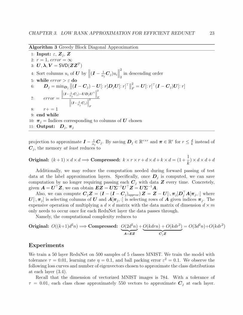
We train a 50 layer ReduNet on 500 samples of 5 classes MNIST. We train the model withtolerance τ = 0.01, learning rate η = 0.1, and ball packing error ε2 = 0.1. We observe thefollowing loss curves and number of eigenvectors chosen to approximate the class distributionsat each layer (3.4).
Recall that the dimension of vectorized MNIST images is 784. With a tolerance ofτ = 0.01, each class chose approximately 550 vectors to approximate Cj at each layer.
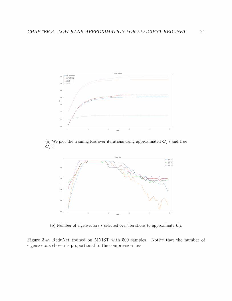
CHAPTER 3. LOW RANK APPROXIMATION FOR EFFICIENT REDUNET 24
0 10 20 30 40 50Layer
100
200
300
400
500
600
700
800
Loss
Layer vs Losslow_diagonal Rlow_diagonal Rlow_diagonal Rc
true Rtrue Rtrue Rc
(a) We plot the training loss over iterations using approximated Cj ’s and trueCj ’s.
0 10 20 30 40 50Layer
535
540
545
550
555
r
Layer vs rclass 0 rclass 1 rclass 2 rclass 3 rclass 4 r
(b) Number of eigenvectors r selected over iterations to approximate Cj .
Figure 3.4: ReduNet trained on MNIST with 500 samples. Notice that the number ofeigenvectors chosen is proportional to the compression loss
CHAPTER 3. LOW RANK APPROXIMATION FOR EFFICIENT REDUNET 25
Additionally, we see that with further training, the number of eigenvectors r needed toapproximate each class’s compression matrix decreases. This is as expected, since at a localminima of the MCR2 objective, the eigenvector of ZZ> become closer to the eigenvectorsof ZjZ
>j , ∀j. However 550 vectors is no where close to d
k= 784
5which implies that that it
is difficult to approximate Zj using a subset of eigenvectors of Z, especially at the initiallayers. Additionally, this suggests it takes a while for Z to converge to an optimal solution.
3.3 Conclusion
From our experiments, we conclude that low rank approximation of the covariance matricesis an efficient way to reduce memory of ReduNet. By setting τ = 0.1 we found a significantreduction in memory footprint in both our experiments in MNIST and CIFAR10 3.3. Forfuture work, it would be interesting to see if we can identify low rank memory reducednetworks for the Convolutional ReduNet [2], whereE andCj are circulant matrices. Additionally,
26
Bibliography
[1] P. Buzzega et al. “Dark Experience for General Continual Learning: a Strong, SimpleBaseline”. In: Adv. Neural Inform. Process. Syst. (2020).
[2] Ryan Chan et al. “Deep Networks from the Principle of Rate Reduction”. In: arXivpreprint arXiv:2010.14765 (2020).
[3] Kaiming He et al. “Deep residual learning for image recognition”. In: IEEE Conf.Comput. Vis. Pattern Recog. (2016).
[4] Geoffrey Hinton, Oriol Vinyals, and Jeff Dean. “Distilling the knowledge in a neuralnetwork”. In: arXiv preprint arXiv:1503.02531 (2015).
[5] Ronald Kemker and Christopher Kanan. “Fearnet: Brain-inspired model for incrementallearning”. In: arXiv preprint arXiv:1711.10563 (2017).
[6] James Kirkpatrick et al. “Overcoming catastrophic forgetting in neural networks”. In:PNAS (2017).
[7] Alex Krizhevsky. “Learning multiple layers of features from tiny images”. In: Technicalreport (2009).
[8] Alex Krizhevsky, Geoffrey Hinton, et al. “Learning multiple layers of features fromtiny images”. In: (2009).
[9] Yann LeCun. “The MNIST database of handwritten digits”. In: http://yann. lecun.com/exdb/mnist/(1998).
[10] Yann LeCun et al. “Gradient-based learning applied to document recognition”. In:Proceedings of the IEEE 86.11 (1998), pp. 2278–2324.
[11] Xilai Li et al. “Learn to grow: A continual structure learning framework for overcomingcatastrophic forgetting”. In: arXiv preprint arXiv:1904.00310 (2019).
[12] Zhizhong Li and Derek Hoiem. “Learning without Forgetting”. In: Eur. Conf. Comput.Vis. (2016).
[13] Yi Ma et al. “Segmentation of multivariate mixed data via lossy data coding andcompression”. In: IEEE transactions on pattern analysis and machine intelligence 29.9(2007), pp. 1546–1562.
BIBLIOGRAPHY 27
[14] Michael McCloskey and Neal J Cohen. “Catastrophic interference in connectionistnetworks: The sequential learning problem”. In: Psychology of learning and motivation.Vol. 24. Elsevier, 1989, pp. 109–165.
[15] Vardan Papyan, X.Y. Han, and David Donoho. “Prevalence of Neural Collapse duringthe Terminal Phase of Deep Learning Training”. In: PNAS (2020).
[16] Sylvestre-Alvise Rebuffi et al. “iCaRL: Incremental Classifier and Representation Learning”.In: IEEE Conf. Comput. Vis. Pattern Recog. (2017).
[17] Andrei A Rusu et al. “Progressive neural networks”. In: arXiv preprint arXiv:1606.04671(2016).
[18] Kate Saenko et al. “Adapting visual category models to new domains”. In: Europeanconference on computer vision. Springer. 2010, pp. 213–226.
[19] Jonathan Schwarz et al. “Progress & Compress: A scalable framework for continuallearning”. In: ICML (2018).
[20] Gido van de Ven and Andreas Tolias. “Three scenarios for continual learning”. In: Adv.Neural Inform. Process. Syst. (2018).
[21] Chenshen Wu et al. “Memory replay gans: Learning to generate new categories withoutforgetting”. In: Advances in Neural Information Processing Systems. 2018, pp. 5962–5972.
[22] Yue Wu et al. “Large scale incremental learning”. In: Proceedings of the IEEE Conferenceon Computer Vision and Pattern Recognition. 2019, pp. 374–382.
[23] Ziyang Wu et al. “Incremental learning via rate reduction”. In: Proceedings of the IEEEConference on Computer Vision and Pattern Recognition (2021).
[24] Lu Yu et al. “Semantic Drift Compensation for Class-Incremental Learning”. In: IEEEConf. Comput. Vis. Pattern Recog. (2020).
[25] Yaodong Yu et al. “Learning Diverse and Discriminative Representations via thePrinciple of Maximal Coding Rate Reduction”. In: Adv. Neural Inform. Process. Syst.(2020).
[26] Friedemann Zenke, Ben Poole, and Surya Ganguli. “Continual Learning ThroughSynaptic Intelligence”. In: ICML (2017).
[27] Junting Zhang et al. “Class-incremental learning via deep model consolidation”. In:The IEEE Winter Conference on Applications of Computer Vision. 2020, pp. 1131–1140.