Dimensionality Reduction via Sparse Support Vector Machines

Journal of Machine Learning Research 1 (2002) 1-48 Submitted 5/02; Published xx/03

Dimensionality Reduction via SparseSupport Vector Machines

Jinbo Bi1 [email protected]

Kristin P. Bennett1 [email protected]

Mark Embrechts2 [email protected]

Curt M. Breneman3 [email protected]

Minghu Song3 [email protected] of Mathematical Sciences2Department of Decision Science and Engineering Systems3Department of ChemistryRensselaer Polytechnic InstituteTroy, NY 12180, USA

Editor: Isabelle Guyon and Andre Elisseeff

Abstract

We describe a methodology for performing variable ranking and selection using supportvector machines (SVMs). The method constructs a series of sparse linear SVMs to generatelinear models that can generalize well, and uses a subset of nonzero weighted variables foundby the linear models to produce a final nonlinear model. The method exploits the fact that alinear SVM (no kernels) with `1-norm regularization inherently performs variable selectionas a side-effect of minimizing capacity of the SVM model. The distribution of the linearmodel weights provides a mechanism for ranking and interpreting the effects of variables.Starplots are used to visualize the magnitude and variance of the weights for each variable.We illustrate the effectiveness of the methodology on synthetic data, benchmark problems,and challenging regression problems in drug design. This method can dramatically reducethe number of variables and outperforms SVMs trained using all attributes and using theattributes selected according to correlation coefficients. The visualization of the resultingmodels is useful for understanding the role of underlying variables.

Keywords: Variable Selection, Dimensionality Reduction, Support Vector Machines,Regression, Pattern Search, Bootstrap Aggregation, Model Visualization

1. Introduction

Variable selection refers to the problem of selecting input variables that are most predictiveof a given outcome. Appropriate variable selection can enhance the effectiveness and domaininterpretability of an inference model. Variable selection problems are found in many su-pervised and unsupervised machine learning tasks including classification, regression, timeseries prediction, clustering, etc. We shall focus on supervised regression tasks, but thegeneral methodology can be extended to any inference task that can be formulated as an`1-norm SVM, such as classification and novelty detection (Campbell and Bennett, 2000,Bennett and Bredensteiner, 1997). The objective of variable selection is two-fold: improv-

c©2002 Jinbo Bi, Kristin Bennett, Mark Embrechts, Curt Breneman and Minghu Song.

Bi, Bennett, Embrechts, Breneman and Song

ing prediction performance (Kittler, 1986) and enhancing understanding of the underlyingconcepts in the induction model.

Our variable selection methodology for SVMs was created to address challenging prob-lems in Quantitative Structural-Activity Relationships (QSAR) analysis. The goal of QSARanalysis is to predict the bioactivity of molecules. Each molecule has many potential de-scriptors (300-1000) that may be highly correlated with each other or irrelevant to the targetbioactivity. The bioactivity is known for only a few molecules (30-200). These issues makemodel validation challenging and overfitting easy. The results of the SVMs are somewhatunstable – small changes in the training and validation data or on model parameters mayproduce rather different sets of nonzero weighted attributes (Breneman et al., 2002). Ourvariable selection and ranking methodology exploits this instability. Computational costsare not a primary issue in our experiments due to lack of data. Our method is based onsparse SVMs, so we call the algorithm VS-SSVM for Variable Selection via Sparse SVMs.

Variable selection is a search problem, with each state in the search space specifying asubset of the possible attributes of the task. Exhaustive evaluation of all variable subsetsis usually intractable. Genetic algorithms, population-based learning, and related Bayesianmethods have been commonly used as search engines for the variable selection process (Inzaet al., 1999, Yang and Honavar, 1997, Kudo et al., 2000). Particularly for SVMs, a variableselection method was introduced (Weston et al., 2000) based on finding the variables thatminimize bounds on the leave-one-out error for classification. The search of variable subsetscan be efficiently performed by a gradient descent algorithm. The method, however, waslimited to separable classification problems, and thus is not directly applicable to the re-gression problems examined in this paper. Guyon et al. proposed another variable selectionmethod for classification by recursively eliminating the input variables that decrease themargin the least (Guyon et al., 2002). A generic wrapper approach based on sensitivityanalysis has been applied to kernel SVM regression (SVR) (Embrechts et al., 2001) but itis more computationally intensive than our proposed approach.

Variable selection methods are often divided along two lines: filter and wrapper methods(Kohavi and John, 1997). The filter approach of selecting variables serves as a preprocessingstep to the induction. The main disadvantage of the filter approach is that it totally ignoresthe effects of the selected variable subset on the performance of the induction algorithm. Thewrapper method searches through the space of variable subsets using the estimated accuracyfrom an induction algorithm as the measure of “goodness” for a particular variable subset.Thus, the variable selection is being “wrapped around” a particular induction algorithm.These methods have encountered some success with induction tasks, but they can be verycomputationally expensive for tasks with a large number of variables.

Our approach (VS-SSVM) consists largely of two consecutive parts: variable selectionand nonlinear induction. The selection of variables serves as a preprocessing step to thefinal kernel SVR induction. The variable selection itself is performed by wrapping aroundlinear SVMs (no kernels) with sparse norm regularization. Such sparse linear SVMs areconstructed to both identify variable subsets and assess their relevance in a computationallycheaper way compared with a direct wrap around nonlinear SVMs. However, the variableselection by linear SVMs and the final nonlinear SVM inference are tightly coupled sincethey both employ the same loss function. Our method is similar in spirit to the Least

2

Dimensionality Reduction via Sparse Support Vector Machines

Absolute Shrinkage and Selection Operator (LASSO) method (Tibshirani, 1994) but isspecifically targeted to SVR with the ε-insensitive loss function.

This article is organized as follows. In Section 2, we review sparse SVMs with `1-normregularization, specifically, the sparse ν-SVR. Section 3 provides details on the VS-SSVMalgorithm based on sparse linear SVMs. Sections 4 and 5 compare VS-SSVM with stepwisedimensionality reduction and correlation coefficient ranking methods on synthetic data andBoston Housing data. Model visualization is also explored in Section 5 to reveal domaininsights. Computational results on real-life QSAR data are included in Section 6.

2. Sparse Support Vector Machines

In this section, we investigate sparse SVMs. Consider the regression problem as finding afunction f∗ ∈ F = {f : Rn → R} that minimizes the regularized risk functional (Boseret al., 1992, Vapnik, 1995, Smola, 1998): R[f ] := P[f ] + C 1

`

∑`i=1 L(yi, f(xi)), where L(·)

is a loss function. Usually the ε-insensitive loss Lε(y, f(x)) = max{|y − f(x)| − ε, 0} isused in SVR. P[·] is a regularization operator and C is called the regularization parameter.For linear functions, f(x) = w′x + b, the regularization operator in classic SVMs is thesquared `2-norm of the normal vector w. Nonlinear functions are produced by mapping xto Φ(x) in a feature space via the kernel function k and constructing linear functions in thefeature space. A linear function in feature space corresponds to a nonlinear function in theoriginal input space. The optimal solution w to SVMs can be expressed as a support vectorexpansion w =

∑αiΦ(xi). Thus, the regression function can be equivalently expressed

as a kernel expansion f(x) =∑

αiΦ(xi)′Φ(x) + b =∑

αik(xi,x) + b. Classic SVMs arequadratic programs (QPs) in terms of α.

Solving QPs is typically computationally more expensive than solving linear programs(LPs). SVMs can be transformed into LPs as in Bennett (1999), Breiman (1999) andSmola et al. (1999). This is achieved by regularizing with a sparse norm, e.g. the `1-norm.This technique is also used in basis pursuit (Chen et al., 1995), parsimonious least normapproximation (Bradley et al., 1998), and LASSO (Tibshirani, 1994). Instead of choosingthe “flattest” function as in classic SVR, we directly apply the `1-norm to the coefficientvector α in the kernel expansion of f . The regularized risk functional is then specified as

R[f ] :=∑

i=1

|αi|+ C1`

∑

i=1

Lε(yi, f(xi)). (1)

This is referred to as a “sparse” SVM because the optimal solution w is usually constructedbased on fewer training examples xi than in classic SVMs and thus the function f requiresfewer kernel entries k(xi,x).

The classic SVR approach has two hyper-parameters C and ε. The tube parameter εcan be difficult to select as one does not know beforehand how accurately the function willfit. The ν-SVR (Scholkopf et al., 2000, Smola et al., 1999) was developed to automaticallyadjust the tube size, ε, by using a parameter ν ∈ (0, 1]. The parameter ν provides anupper bound on the fraction of error examples and a lower bound on the fraction of supportvectors. To form the ν-SVR LP, we rewrite αj = uj − vj where uj , vj ≥ 0. The solutionhas either uj or vj equal to 0, depending on the sign of αj , so |αj | = uj + vj . Let the

3


training data be (xi, yi), i = 1, · · · , ` where xi ∈ Rn with the jth component of xi denotedas xij , j = 1, · · · , n. The LP is formulated in variables u, v, b, ε, ξ and η as

min∑

j=1

(uj + vj) + C1`

∑

i=1

(ξi + ηi) + Cνε

s.t. yi −∑j=1

(uj − vj) k(xi,xj)− b ≤ ε + ξi, i = 1, . . . , `,

∑j=1

(uj − vj) k(xi,xj) + b− yi ≤ ε + ηi, i = 1, . . . , `,

uj , vj , ξi, ηi, ε ≥ 0, i, j = 1, . . . , `.

(2)

LP (2) provides the basis of both our variable selection and modeling methods. To selectvariables effectively, we employ a sparse linear SVR which is formulated from LP (2) simplyby replacing k(xi,xj) by xij with index i running over examples and index j running overvariables. The optimal solution is then given by w = u−v. To construct the final nonlinearmodel, we use the sparse nonlinear SVR LP(2) with a nonlinear kernel such as the RBFkernel k(x, z) = exp

(−||x−z||2σ2

). The optimal solution is then given by α = u− v.

3. The VS-SSVM Algorithm

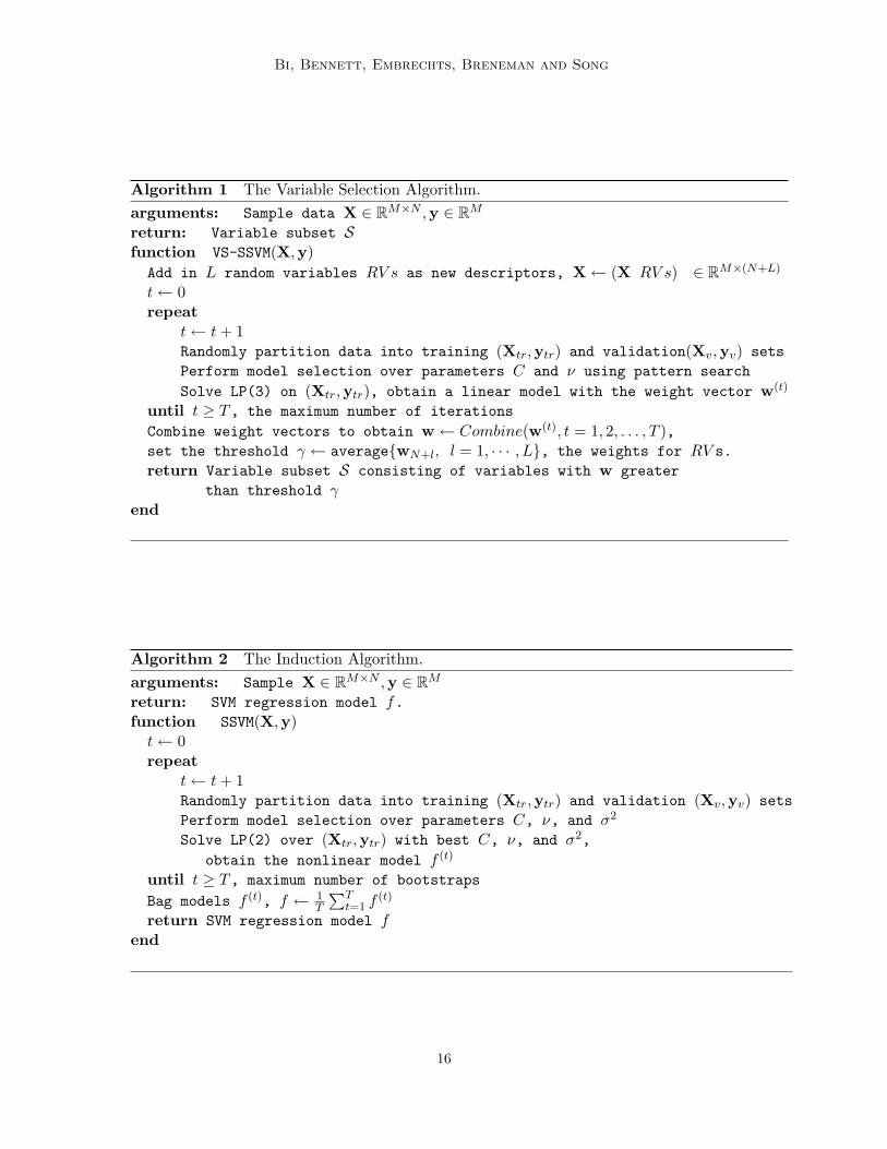
We briefly describe the VS-SSVM algorithm in this section. The VS-SSVM algorithmconsists of 5 essential components: 1. A linear model with sparse w constructed by solvinga linear SVM LP to obtain a subset of variables nonzero-weighted in the linear model; 2. Anefficient search for optimal hyper-parameters C and ν in the linear SVM LP using “patternsearch”; 3. The use of bagging to reduce the variability of variable selection; 4. A methodfor discarding the least significant variables by comparing them to “random” variables; 5.A nonlinear regression model created by training and bagging the LPs (2) with RBF kernelson the final subset of variables selected. We shall explain the various components in moredetail in this section1. Pseudocode for the first four steps is given in Algorithm 1 in theappendix. Algorithm 2 in the appendix describes the final nonlinear regression modelingalgorithm. In Section 5, we describe how further filtering of variables can be achieved byvisualizing the bagged solutions and applying rules to the bagged models.

Sparse linear models: Sparse linear models are constructed using the following LP:

minn∑

j=1

(uj + vj) + C1`

∑

i=1

(ξi + ηi) + Cνε

s.t. yi −n∑

j=1(uj − vj) xij − b ≤ ε + ξi, i = 1, . . . , `,

n∑j=1

(uj − vj) xij + b− yi ≤ ε + ηi, i = 1, . . . , `,

uj , vj , ξi, ηi, ε ≥ 0, i = 1, . . . , `, j = 1, . . . , n.

(3)

Let w = u − v be the solution to the linear SVR LP (3). The magnitude and sign ofthe component wj indicates the effect of the jth variable on the model. If wj > 0, the

1. More details are available at the website http://www.rpi.edu/˜bij2/featsele.html

4


variable contributes to y; if wj < 0, the variable reduces y. The `1-norm of w inherently en-forces sparseness of the solution. Roughly speaking, the vectors further from the coordinateaxes are “larger” with respect to the `1-norm than with respect to `p-norms with p > 1.For example, consider the vectors (1, 0) and (1/

√2, 1/

√2). For the `2-norm, ‖(1, 0)‖2 =

‖(1/√2, 1/√

2)‖2 = 1, but for the `1-norm, 1 = ‖(1, 0)‖1 < ‖(1/√2, 1/√

2)‖1 =√

2. Thedegree of sparsity of the solution w depends on the regularization parameter C and thetube parameter ν in LP(3).

Pattern search: Since the hyper-parameters play a crucial role in our variable selec-tion approach, we optimize them using a pattern search approach. This optimization isautomatically performed based on validation set results by applying the derivative-free pat-tern search method (Dennis and Torczon, 1994) in the C-ν search space. For each choiceof C-ν, LP (3) generates a linear model based on the training data. Then the resultingmodel is applied to the validation data and evaluated using the statistic Q2 =

P(yi−yi)

2P(yi−y)2

,the mean squared error scaled by the variance of the response, where yi is the predictionof yi for the ith validation example and y is the mean of the actual responses. The pat-tern search method optimizes this validation Q2 over the C-ν space. A good range for thehyper-parameters may be problem-specific, but we prefer to a generic approach applicableto most datasets. Hence a reasonably large range is adopted to produce the C-ν space,specifically, C ∈ [e−2 = 0.1353, e10 = 22026] and ν ∈ [0.02, 0.6].

The pattern search algorithm is embedded in Algorithm 1 as a sub-routine. Each itera-tion of a pattern search algorithm starts with a center (initially randomly chosen), samplesother points around the center in the search space, and calculates objective values of eachneighboring point until it finds a point with objective value less than that of the center. Thealgorithm then moves the center to the new minimizer. If all the points around the centerfail to bring a decrease to the objective, the search step (used to determine the neighboringpoints) is reduced by half. This search continues until the search step gets sufficiently small,thus ensuring convergence to a local minimizer. For a full explanation of pattern search forSVR see Momma and Bennett (2002).

Variability reduction: The optimal weight vectors w for LP (3) exhibit considerablevariance due to local minima in the pattern search, the small dataset size, and changesin validation data. Different partitions of data may produce very different answers. Noindividual model can be considered completely reliable, especially for QSAR data. Thus“bootstrap aggregation” or “bagging” is used to make the procedure more stable (Breiman,1996). In our experiments, models were constructed based on T = 20 random partitions toproduce distinct weight vectors. There are several schemes to combine models. We tookthe superset of nonzero weighted variables obtained in any of the 20 different partitions– the “bagged” subset of the variables. Bagging can augment the performance of variousindividual models due to the reduced variance of the “bagged” model (Breiman, 1996).For problems with large variance, regression based on the average usually outperforms anysingle model. We use bagging for both variable selection and nonlinear SVR modeling.

Discarding least significant variables: Sparsity of the linear model eliminates manyvariables in every bootstrap, but it is possible that in any given bootstrap irrelevant variablesare included. Thus, we also eliminate variables by introducing random gauge variables. Theintuition is that if an independent variable has even less significance than a random variablewhich is barely related to the response, then it may be safely deleted. The VS-SSVM

5


Algorithm 1 first augments the data with normally distributed random variables (mean0 and standard deviation 1). Random variables following other distributions can also beemployed. See Stoppiglia and Dreyfus (2003) for a more thorough discussion of this issue.Based on the previous empirical results in Embrechts et al. (2001), we added 3 randomvariables with sample correlations to the response less than 0.13 in magnitude. The weightsw for these random variables provide clues for thresholding the selection of variables basedon the average of the weights on the 3 variables across all the bootstraps. Only variableswith average weight greater than this average will be selected. The selection of variablescan be further refined. We leave the explanation of our scheme for model visualization andfurther filtering of the variables until Section 5.

Nonlinear SVR models: After the final set of variables is selected, we employ Al-gorithm 2 in the appendix to construct the nonlinear SVR model. Nonlinear models wereconstructed based on T = 10 partitions and then averaged to produce the final model. Wefocus on evaluating the performance of the variable selection method more than optimizingthe predictor. Hence a simple grid search was used in nonlinear SVR modeling to selecthyper-parameters rather than pattern search in each fold of the bagging. In the grid search,we considered only the RBF kernels with parameter σ2 equal to 8, 100, 150, 250, 500, 1000,3000, 5000, and 10000. The parameter C was chosen from values between 10 and 20000with 100 as the increment within 1000 and 1000 as the increment from 1000 to 20000, andthe parameter ν from 0.1, 0.15, 0.2, 0.3, and 0.5.

4. Computational Analysis of VS-SSVM

We evaluated the computational effectiveness of VS-SSVM on synthetic data and the bench-mark Boston Housing problem (Harrison and Rubinfeld, 1978). Our goal was to examinewhether VS-SSVM can improve generalization. The LPs (2) and (3) formulated on trainingdata were both solved using CPLEX version 6.6 (ILOG, 1999).

We compared VS-SSVM with a widely used method, “stepwise regression” wrappedaround Generalized Linear Models (GLM) (Miller, 1990). For fair comparison, the GLMmodels were also bagged. Hence 20 different GLM models were generated using Splus 2000(Venables and Ripley, 1994, McCullagh and Nelder, 1983) based on different bootstrappedsamples, and the resulting models were bagged. The bagged models performed at least aswell as single models, so only the bagged results are presented here. In each trial, half ofthe examples were held out for test and the other half were used in training. VS-SSVM andstepwise regression were run on the training data. The training data were further dividedto create a validation set in each fold of the bagging scheme. The final models were appliedto the hold-out test data in order to compute the test Q2. This procedure was repeated 20times on different training-test splits of the data for both methods.

The synthetic data set was randomly generated with solution pre-specified as follows:there are 12 independent variables and 1 response variable. The first 5 variables, x1, . . . , x5,were drawn independently and identically distributed from the standard normal distribu-tion. The 6th variable was x6 = x1 + 1 which is correlated to x1. The 7th variable wasx7 = x2x3 which relates to both x2 and x3. Five additional standard normally distributedvariables were also generated, and had nothing to do with the dependent y. We call them

6


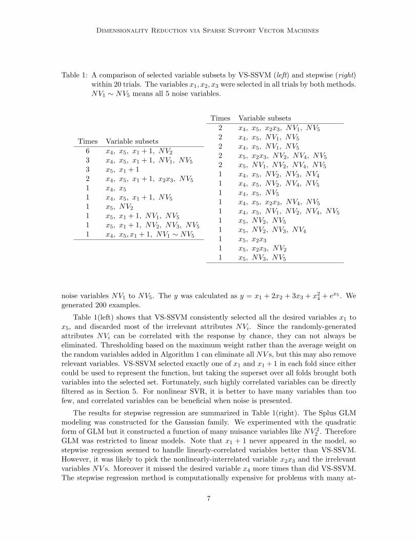
Table 1: A comparison of selected variable subsets by VS-SSVM (left) and stepwise (right)within 20 trials. The variables x1, x2, x3 were selected in all trials by both methods.NV1 ∼ NV5 means all 5 noise variables.

Times Variable subsets6 x4, x5, x1 + 1, NV2

3 x4, x5, x1 + 1, NV1, NV5

3 x5, x1 + 12 x4, x5, x1 + 1, x2x3, NV5

1 x4, x5

1 x4, x5, x1 + 1, NV5

1 x5, NV2

1 x5, x1 + 1, NV1, NV5

1 x5, x1 + 1, NV2, NV3, NV5

1 x4, x5, x1 + 1, NV1 ∼ NV5

Times Variable subsets2 x4, x5, x2x3, NV1, NV5

2 x4, x5, NV1, NV5

2 x4, x5, NV1, NV5

2 x5, x2x3, NV2, NV4, NV5

2 x5, NV1, NV2, NV4, NV5

1 x4, x5, NV2, NV3, NV4

1 x4, x5, NV2, NV4, NV5

1 x4, x5, NV5

1 x4, x5, x2x3, NV4, NV5

1 x4, x5, NV1, NV2, NV4, NV5

1 x5, NV2, NV5

1 x5, NV2, NV3, NV4

1 x5, x2x3

1 x5, x2x3, NV2

1 x5, NV3, NV5

noise variables NV1 to NV5. The y was calculated as y = x1 + 2x2 + 3x3 + x24 + ex5 . We

generated 200 examples.

Table 1(left) shows that VS-SSVM consistently selected all the desired variables x1 tox5, and discarded most of the irrelevant attributes NVi. Since the randomly-generatedattributes NVi can be correlated with the response by chance, they can not always beeliminated. Thresholding based on the maximum weight rather than the average weight onthe random variables added in Algorithm 1 can eliminate all NV s, but this may also removerelevant variables. VS-SSVM selected exactly one of x1 and x1 + 1 in each fold since eithercould be used to represent the function, but taking the superset over all folds brought bothvariables into the selected set. Fortunately, such highly correlated variables can be directlyfiltered as in Section 5. For nonlinear SVR, it is better to have many variables than toofew, and correlated variables can be beneficial when noise is presented.

The results for stepwise regression are summarized in Table 1(right). The Splus GLMmodeling was constructed for the Gaussian family. We experimented with the quadraticform of GLM but it constructed a function of many nuisance variables like NV 2

2 . ThereforeGLM was restricted to linear models. Note that x1 + 1 never appeared in the model, sostepwise regression seemed to handle linearly-correlated variables better than VS-SSVM.However, it was likely to pick the nonlinearly-interrelated variable x2x3 and the irrelevantvariables NV s. Moreover it missed the desired variable x4 more times than did VS-SSVM.The stepwise regression method is computationally expensive for problems with many at-

7


−10 −5 0 5 10

−10

−5

0

5

10

SCATTERPLOT DATA ( VS−SSVM on Synthetic)

Observed Response

Pred

icte

d R

espo

nse

r2 = 0.9678 Q2 = 0.0332 Std(Q2) = 0.0027

−10 −5 0 5 10

−10

−5

0

5

10

SCATTERPLOT DATA ( GLM on Synthetic )

Observed Response

Pred

icte

d R

espo

nse

r2 = 0.8713 Q2 = 0.1287 Std(Q2) = 0.0065

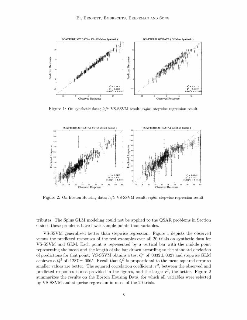
Figure 1: On synthetic data; left: VS-SSVM result; right: stepwise regression result.

5 10 15 20 25 30 35 40 45 50 555

10

15

20

25

30

35

40

45

50

55

SCATTERPLOT DATA ( VS−SSVM on Boston )

Observed Response

Pred

icte

d R

espo

nse

r2 = 0.8295 Q2 = 0.1713 Std(Q2) = 0.0093

0 5 10 15 20 25 30 35 40 45 50

0

5

10

15

20

25

30

35

40

45

50SCATTERPLOT DATA ( GLM on Boston )

Observed Response

Pred

icte

d R

espo

nse

r2 = 0.6848 Q2 = 0.3171 Std(Q2) = 0.0126

Figure 2: On Boston Housing data; left: VS-SSVM result; right: stepwise regression result.

tributes. The Splus GLM modeling could not be applied to the QSAR problems in Section6 since these problems have fewer sample points than variables.

VS-SSVM generalized better than stepwise regression. Figure 1 depicts the observedversus the predicted responses of the test examples over all 20 trials on synthetic data forVS-SSVM and GLM. Each point is represented by a vertical bar with the middle pointrepresenting the mean and the length of the bar drawn according to the standard deviationof predictions for that point. VS-SSVM obtains a test Q2 of .0332±.0027 and stepwise GLMachieves a Q2 of .1287± .0065. Recall that Q2 is proportional to the mean squared error sosmaller values are better. The squared correlation coefficient, r2, between the observed andpredicted responses is also provided in the figures, and the larger r2, the better. Figure 2summarizes the results on the Boston Housing Data, for which all variables were selectedby VS-SSVM and stepwise regression in most of the 20 trials.

8


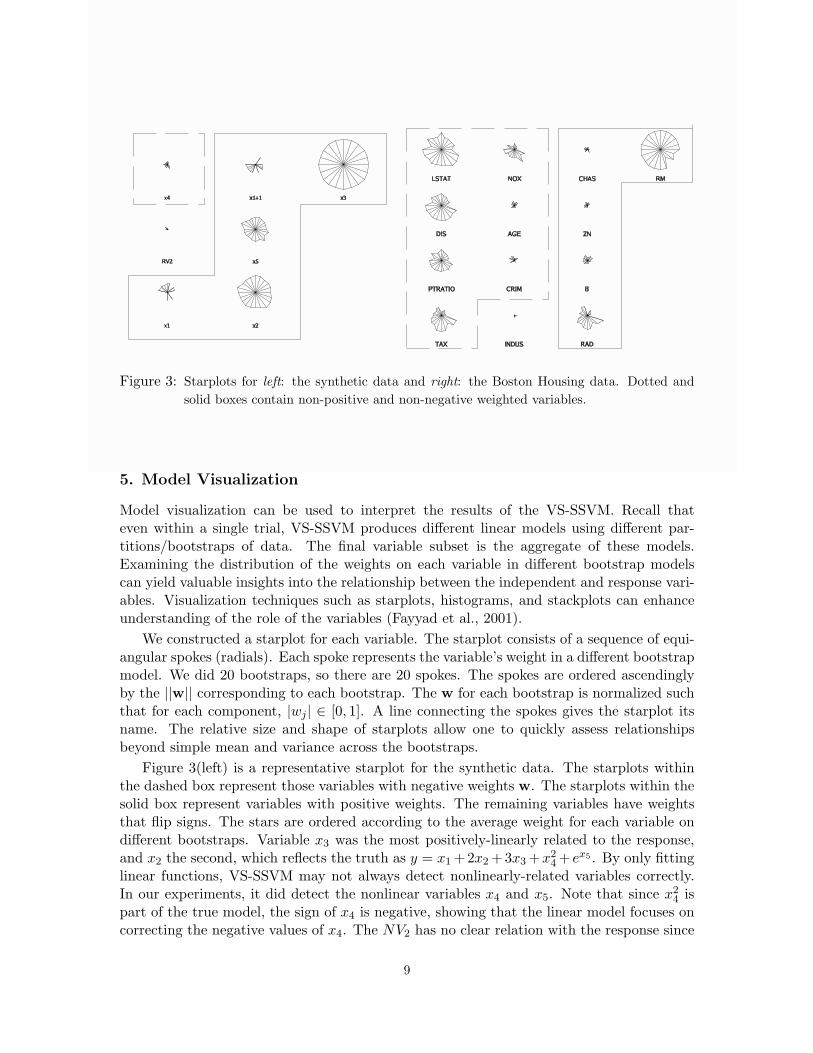
Figure 3: Starplots for left: the synthetic data and right: the Boston Housing data. Dotted andsolid boxes contain non-positive and non-negative weighted variables.

5. Model Visualization

Model visualization can be used to interpret the results of the VS-SSVM. Recall thateven within a single trial, VS-SSVM produces different linear models using different par-titions/bootstraps of data. The final variable subset is the aggregate of these models.Examining the distribution of the weights on each variable in different bootstrap modelscan yield valuable insights into the relationship between the independent and response vari-ables. Visualization techniques such as starplots, histograms, and stackplots can enhanceunderstanding of the role of the variables (Fayyad et al., 2001).

We constructed a starplot for each variable. The starplot consists of a sequence of equi-angular spokes (radials). Each spoke represents the variable’s weight in a different bootstrapmodel. We did 20 bootstraps, so there are 20 spokes. The spokes are ordered ascendinglyby the ||w|| corresponding to each bootstrap. The w for each bootstrap is normalized suchthat for each component, |wj | ∈ [0, 1]. A line connecting the spokes gives the starplot itsname. The relative size and shape of starplots allow one to quickly assess relationshipsbeyond simple mean and variance across the bootstraps.

Figure 3(left) is a representative starplot for the synthetic data. The starplots withinthe dashed box represent those variables with negative weights w. The starplots within thesolid box represent variables with positive weights. The remaining variables have weightsthat flip signs. The stars are ordered according to the average weight for each variable ondifferent bootstraps. Variable x3 was the most positively-linearly related to the response,and x2 the second, which reflects the truth as y = x1 +2x2 +3x3 +x2

4 + ex5 . By only fittinglinear functions, VS-SSVM may not always detect nonlinearly-related variables correctly.In our experiments, it did detect the nonlinear variables x4 and x5. Note that since x2

4 ispart of the true model, the sign of x4 is negative, showing that the linear model focuses oncorrecting the negative values of x4. The NV2 has no clear relation with the response since

9


the weights for NV2 flip signs among different models. The strategy of removing variableswith flipping signs can further refine variable selection.

The variables with flipping signs do not always coincide with the variables that are leastcorrelated with the response. On the synthetic data the correlation coefficients r of thevariables and the response are:

x1 x2 x3 x4 x5 x1 + 1 NV2

0.233 0.498 0.711 -0.077 0.506 0.233 -0.080

Removing all variables with r less than 0.08 in magnitude would also delete x4.The size and shape of the starplots provide information about the models. The starplots

for variable x1 and x1 +1 are complementary, which means if a bootstrap model selects x1,it does not include x1 +1. The starplots help spot such complementary behavior in models.Hence highly correlated variables can be further filtered.

VS-SSVM with model visualization can be valuable even on datasets where variableselection does not eliminate variables. For example, on the Boston Housing data, VS-SSVM does not drop any variables. However, the weights produced by VS-SSVM can helpunderstand the role and the relative importance of the variables in the model. The starplotsbased on the entire Boston Housing data are given in Figure 3(right). They are drawn inthe same way as for the synthetic data. For instance, the RM (average number of roomsper dwelling) is the most positively related to the housing price, which reflects that thenumber of rooms is important for determining the housing price and the more rooms thehouse has, the higher the price. The INDUS (proportion of non-retail business acres pertown) appears not to affect the housing price significantly in the linear modeling since thecorresponding weights flip signs.

6. Generalization Testing on QSAR Datasets

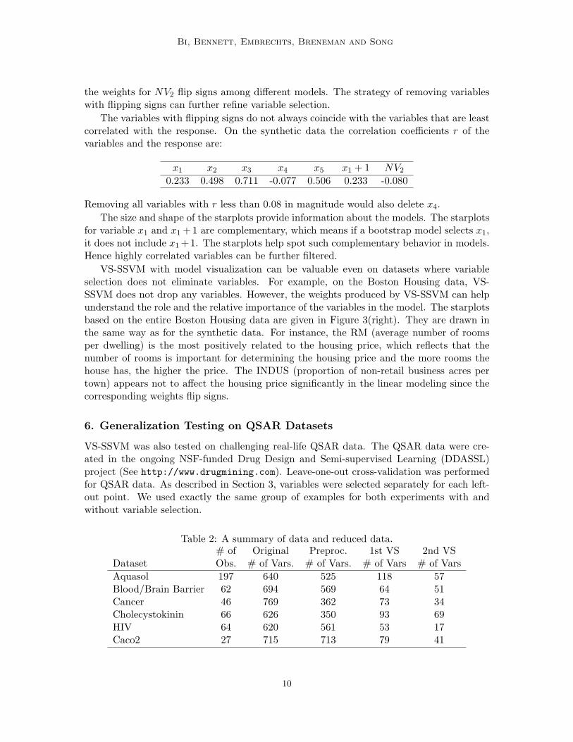
VS-SSVM was also tested on challenging real-life QSAR data. The QSAR data were cre-ated in the ongoing NSF-funded Drug Design and Semi-supervised Learning (DDASSL)project (See http://www.drugmining.com). Leave-one-out cross-validation was performedfor QSAR data. As described in Section 3, variables were selected separately for each left-out point. We used exactly the same group of examples for both experiments with andwithout variable selection.

Table 2: A summary of data and reduced data.# of Original Preproc. 1st VS 2nd VS

Dataset Obs. # of Vars. # of Vars. # of Vars # of VarsAquasol 197 640 525 118 57Blood/Brain Barrier 62 694 569 64 51Cancer 46 769 362 73 34Cholecystokinin 66 626 350 93 69HIV 64 620 561 53 17Caco2 27 715 713 79 41

10


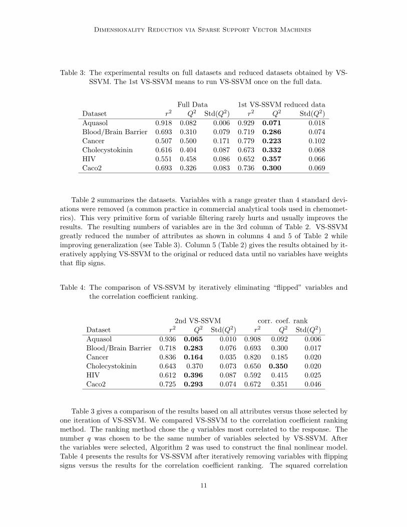
Table 3: The experimental results on full datasets and reduced datasets obtained by VS-SSVM. The 1st VS-SSVM means to run VS-SSVM once on the full data.

Full Data 1st VS-SSVM reduced dataDataset r2 Q2 Std(Q2) r2 Q2 Std(Q2)Aquasol 0.918 0.082 0.006 0.929 0.071 0.018Blood/Brain Barrier 0.693 0.310 0.079 0.719 0.286 0.074Cancer 0.507 0.500 0.171 0.779 0.223 0.102Cholecystokinin 0.616 0.404 0.087 0.673 0.332 0.068HIV 0.551 0.458 0.086 0.652 0.357 0.066Caco2 0.693 0.326 0.083 0.736 0.300 0.069

Table 2 summarizes the datasets. Variables with a range greater than 4 standard devi-ations were removed (a common practice in commercial analytical tools used in chemomet-rics). This very primitive form of variable filtering rarely hurts and usually improves theresults. The resulting numbers of variables are in the 3rd column of Table 2. VS-SSVMgreatly reduced the number of attributes as shown in columns 4 and 5 of Table 2 whileimproving generalization (see Table 3). Column 5 (Table 2) gives the results obtained by it-eratively applying VS-SSVM to the original or reduced data until no variables have weightsthat flip signs.

Table 4: The comparison of VS-SSVM by iteratively eliminating “flipped” variables andthe correlation coefficient ranking.

2nd VS-SSVM corr. coef. rankDataset r2 Q2 Std(Q2) r2 Q2 Std(Q2)Aquasol 0.936 0.065 0.010 0.908 0.092 0.006Blood/Brain Barrier 0.718 0.283 0.076 0.693 0.300 0.017Cancer 0.836 0.164 0.035 0.820 0.185 0.020Cholecystokinin 0.643 0.370 0.073 0.650 0.350 0.020HIV 0.612 0.396 0.087 0.592 0.415 0.025Caco2 0.725 0.293 0.074 0.672 0.351 0.046

Table 3 gives a comparison of the results based on all attributes versus those selected byone iteration of VS-SSVM. We compared VS-SSVM to the correlation coefficient rankingmethod. The ranking method chose the q variables most correlated to the response. Thenumber q was chosen to be the same number of variables selected by VS-SSVM. Afterthe variables were selected, Algorithm 2 was used to construct the final nonlinear model.Table 4 presents the results for VS-SSVM after iteratively removing variables with flippingsigns versus the results for the correlation coefficient ranking. The squared correlation

11


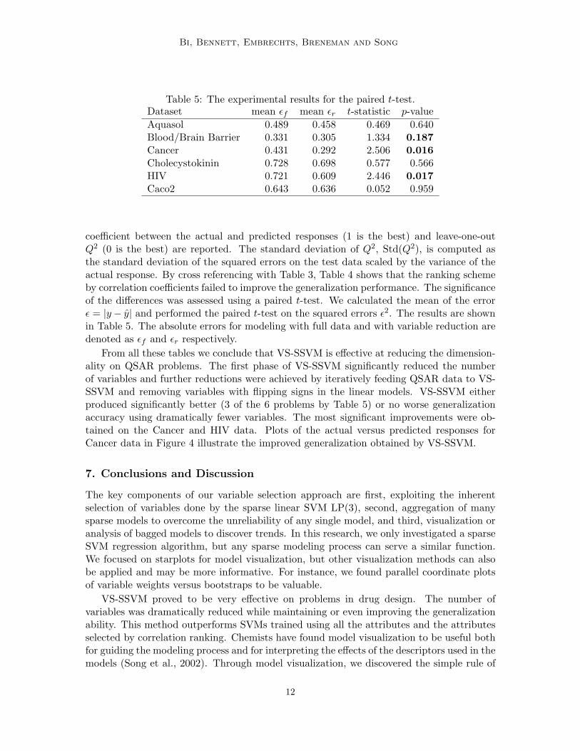
Table 5: The experimental results for the paired t-test.Dataset mean εf mean εr t-statistic p-valueAquasol 0.489 0.458 0.469 0.640Blood/Brain Barrier 0.331 0.305 1.334 0.187Cancer 0.431 0.292 2.506 0.016Cholecystokinin 0.728 0.698 0.577 0.566HIV 0.721 0.609 2.446 0.017Caco2 0.643 0.636 0.052 0.959

coefficient between the actual and predicted responses (1 is the best) and leave-one-outQ2 (0 is the best) are reported. The standard deviation of Q2, Std(Q2), is computed asthe standard deviation of the squared errors on the test data scaled by the variance of theactual response. By cross referencing with Table 3, Table 4 shows that the ranking schemeby correlation coefficients failed to improve the generalization performance. The significanceof the differences was assessed using a paired t-test. We calculated the mean of the errorε = |y− y| and performed the paired t-test on the squared errors ε2. The results are shownin Table 5. The absolute errors for modeling with full data and with variable reduction aredenoted as εf and εr respectively.

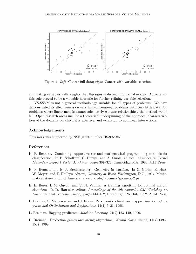
From all these tables we conclude that VS-SSVM is effective at reducing the dimension-ality on QSAR problems. The first phase of VS-SSVM significantly reduced the numberof variables and further reductions were achieved by iteratively feeding QSAR data to VS-SSVM and removing variables with flipping signs in the linear models. VS-SSVM eitherproduced significantly better (3 of the 6 problems by Table 5) or no worse generalizationaccuracy using dramatically fewer variables. The most significant improvements were ob-tained on the Cancer and HIV data. Plots of the actual versus predicted responses forCancer data in Figure 4 illustrate the improved generalization obtained by VS-SSVM.

7. Conclusions and Discussion

The key components of our variable selection approach are first, exploiting the inherentselection of variables done by the sparse linear SVM LP(3), second, aggregation of manysparse models to overcome the unreliability of any single model, and third, visualization oranalysis of bagged models to discover trends. In this research, we only investigated a sparseSVM regression algorithm, but any sparse modeling process can serve a similar function.We focused on starplots for model visualization, but other visualization methods can alsobe applied and may be more informative. For instance, we found parallel coordinate plotsof variable weights versus bootstraps to be valuable.

VS-SSVM proved to be very effective on problems in drug design. The number ofvariables was dramatically reduced while maintaining or even improving the generalizationability. This method outperforms SVMs trained using all the attributes and the attributesselected by correlation ranking. Chemists have found model visualization to be useful bothfor guiding the modeling process and for interpreting the effects of the descriptors used in themodels (Song et al., 2002). Through model visualization, we discovered the simple rule of

12


2.5 3 3.5 4 4.5 5 5.5 6 6.5 7

2.5

3

3.5

4

4.5

5

5.5

6

6.5

7

SCATTERPLOT DATA ( All attributes )

Observed Response

Pred

icte

d R

espo

nse

r2 = 0.5073 Q2 = 0.5008 Std(Q2) = 0.1713

2.5 3 3.5 4 4.5 5 5.5 6 6.5 7

2.5

3

3.5

4

4.5

5

5.5

6

6.5

7

SCATTERPLOT DATA ( VS−SSVM on Cancer )

Observed Response

Pred

icte

d R

espo

nse

r2 = 0.7782 Q2 = 0.2232 Std(Q2) = 0.1021

Figure 4: Left: Cancer full data; right: Cancer with variable selection.

eliminating variables with weights that flip signs in distinct individual models. Automatingthis rule proved to be a valuable heuristic for further refining variable selection.

VS-SSVM is not a general methodology suitable for all types of problems. We havedemonstrated its effectiveness on very high-dimensional problems with very little data. Onproblems where linear models cannot adequately capture relationships, the method wouldfail. Open research areas include a theoretical underpinning of the approach, characteriza-tion of the domains on which it is effective, and extension to nonlinear interactions.

Acknowledgements

This work was supported by NSF grant number IIS-9979860.

References

K. P. Bennett. Combining support vector and mathematical programming methods forclassification. In B. Scholkopf, C. Burges, and A. Smola, editors, Advances in KernelMethods – Support Vector Machines, pages 307–326, Cambridge, MA, 1999. MIT Press.

K. P. Bennett and E. J. Bredensteiner. Geometry in learning. In C. Gorini, E. Hart,W. Meyer, and T. Phillips, editors, Geometry at Work, Washington, D.C., 1997. Mathe-matical Association of America. www.rpi.edu/∼bennek/geometry2.ps.

B. E. Boser, I. M. Guyon, and V. N. Vapnik. A training algorithm for optimal marginclassifiers. In D. Haussler, editor, Proceedings of the 5th Annual ACM Workshop onComputational Learning Theory, pages 144–152, Pittsburgh, PA, July 1992. ACM Press.

P. Bradley, O. Mangasarian, and J. Rosen. Parsimonious least norm approximation. Com-putational Optimization and Applications, 11(1):5–21, 1998.

L. Breiman. Bagging predictors. Machine Learning, 24(2):123–140, 1996.

L. Breiman. Prediction games and arcing algorithms. Neural Computation, 11(7):1493–1517, 1999.

13


C. Breneman, K. Bennett, M. Embrechts, S. Cramer, M. Song, and J. Bi. Descriptorgeneration, selection and model building in quantitative structure-property analysis. InJ. Crawse, editor, Experimental Design for Combinatorial and High Throughput MaterialsDevelopment. Wiley, 2002.

C. Campbell and K. P. Bennett. A linear programming approach to novelty detection. InNeural Information Processing Systems, volume 13, pages 395–401, 2000.

S. Chen, D. Donoho, and M. Saunders. Atomic decomposition by basis pursuit. TechnicalReport 479, Department of Statistics, Stanford University, May 1995.

J. Dennis and V. Torczon. Derivative-free pattern search methods for multidisciplinarydesign problems. In The Fifth AIAA/USAF/NASA/ISSMO Symposium on Multidisci-plinary Analysis and Optimization, pages 922–932, Americal Institute of Aeronautics andAstronautics, Reston, Virginia, 1994.

M. J. Embrechts, F. A. Arciniegas, M. Ozdemir, C. M. Breneman, and K. P. Bennett.Bagging neural network sensitivity analysis for feature reduction in QSAR problems. InProceedings of 2001 INNS - IEEE International Joint Conference on Neural Networks,volume 4, pages 2478–2482, Washington D. C., 2001. IEEE Press.

U. Fayyad, G. Grinstein, and A. Wierse. Information Visualization in Data Mining andKnowledge Discovery. Morgan Kaufmann, 2001.

I. Guyon, J. Weston, S. Barnhill, and V. Vapnik. Gene selection for cancer classificationusing support vector machines. Machine Learning, 46:389–422, 2002.

D. Harrison and D. L. Rubinfeld. Hedonic prices and the demand for clean air. Journal ofEnviron. Economics and Management, 5:81–102, 1978.

ILOG. ILOG CPLEX 6.5 Reference Manual. ILOG CPLEX Division, Incline Village,Nevada, 1999.

I. Inza, M. Merino, P. Larranaga, J. Quiroga, B. Sierra, and M. Girala. Feature subsetselection by population-based incremental learning. Technical Report no. EHU-KZAA-IK-1/99, University of the Basque Country, Spain, 1999.

J. Kittler. Feature selection and extraction. In T. Y. Young and K.-S. Fu, editors, Handbookof Pattern Recognition and Image Processing. Academic Press, New York, 1986.

R. Kohavi and G. H. John. Wrappers for feature subset selection. Artificial Intelligence,1997(1 - 2):273 – 323, 1997.

M. Kudo, P. Somol, P. Pudil, M. Shimbo, and J. Sklansky. Comparison of classifier-specificfeature selection algorithms. In SSPR/SPR, pages 677–686, 2000.

P. McCullagh and J. A. Nelder. Generalized Linear Models. Chapman and Hall, London,1983.

A. J. Miller. Subset selection in regression. In Monographs on Statistics and AppliedProbability 40. London: Chapman and Hall, 1990.

14


M. Momma and K. P. Bennett. A pattern search method for model selection of supportvector regression. In Proceedings of the SIAM International Conference on Data Mining,Philadelphia, Pennsylvania, 2002. SIAM.

B. Scholkopf, A. Smola, R. C. Williamson, and P. L. Bartlett. New support vector algo-rithms. Neural Computation, 12:1207 – 1245, 2000.

A. J. Smola. Learning with Kernels. PhD thesis, Technische Universitat Berlin, 1998.

A.J. Smola, B. Scholkopf, and G. Ratsch. Linear programs for automatic accuracy controlin regression. In Proceedings ICANN’99, Int. Conf. on Artificial Neural Networks, Berlin,1999. Springer.

M. Song, C. Breneman, J. Bi, N. Sukumar, K. Bennett, S. Cramer, and N. Tugcu. Predictionof protein retention times in anion-exchange chromatography systems using support vec-tor machines. Journal of Chemical Information and Computer Science, 42(6):1347–1357,2002.

H. Stoppiglia and G. Dreyfus. Ranking a random feature for variable and feature selection.Journal of Machine Learning Research, Special Issue on Variable/Feature Selection, 2003.to appear in this issue.

R. Tibshirani. Regression selection and shrinkage via the lasso. Technical report, StatisticsDepartment, Stanford, CA, June 1994.

V. N. Vapnik. The Nature of Statistical Learning Theory. Springer, New York, 1995.

W. N. Venables and B. D. Ripley. Modern Applied Statistics with S-Plus. Springer, NewYork, 1994.

J. Weston, S. Mukherjee, O. Chapelle, M. Pontil, T. Poggio, and V. Vapnik. Featureselection for SVMs. In Neural Information Processing Systems, volume 13, pages 668–674, 2000.

J. Yang and V. Honavar. Feature subset selection using a genetic algorithm. In J. Koza,K. Deb, M. Dorigo, D. Fogel, M. Garzon, H. Iba, and R. Riolo, editors, Genetic Program-ming 1997: Proceedings of the Second Annual Conference, page 380, Stanford University,CA, USA, 1997. Morgan Kaufmann.

Appendix

15


Algorithm 1 The Variable Selection Algorithm.arguments: Sample data X ∈ RM×N ,y ∈ RM

return: Variable subset Sfunction VS-SSVM(X,y)

Add in L random variables RV s as new descriptors, X ← (X RV s) ∈ RM×(N+L)

t ← 0repeat

t ← t + 1Randomly partition data into training (Xtr,ytr) and validation(Xv,yv) setsPerform model selection over parameters C and ν using pattern searchSolve LP(3) on (Xtr,ytr), obtain a linear model with the weight vector w(t)

until t ≥ T, the maximum number of iterationsCombine weight vectors to obtain w ← Combine(w(t), t = 1, 2, . . . , T ),set the threshold γ ← average{wN+l, l = 1, · · · , L}, the weights for RV s.return Variable subset S consisting of variables with w greater

than threshold γend

Algorithm 2 The Induction Algorithm.arguments: Sample X ∈ RM×N ,y ∈ RM

return: SVM regression model f.function SSVM(X,y)

t ← 0repeat

t ← t + 1Randomly partition data into training (Xtr,ytr) and validation (Xv,yv) setsPerform model selection over parameters C, ν, and σ2

Solve LP(2) over (Xtr,ytr) with best C, ν, and σ2,obtain the nonlinear model f (t)

until t ≥ T, maximum number of bootstraps

Bag models f (t), f ← 1T

∑Tt=1 f (t)

return SVM regression model fend

16

Documents

Dimensionality Reduction via Sparse Support Vector Machines