Increasing the Sustainability of Rural Water Service

Policy Research Working Paper 8283

Increasing the Sustainability of Rural Water Service

Findings from the Impact Evaluation Baseline Survey in Nicaragua

Christian Borja-Vega Joshua Gruber

Alexander Spevack

Water Global Practice GroupDecember 2017

WPS8283P

ublic

Dis

clos

ure

Aut

horiz

edP

ublic

Dis

clos

ure

Aut

horiz

edP

ublic

Dis

clos

ure

Aut

horiz

edP

ublic

Dis

clos

ure

Aut

horiz

ed

Produced by the Research Support Team

Abstract

The Policy Research Working Paper Series disseminates the findings of work in progress to encourage the exchange of ideas about development issues. An objective of the series is to get the findings out quickly, even if the presentations are less than fully polished. The papers carry the names of the authors and should be cited accordingly. The findings, interpretations, and conclusions expressed in this paper are entirely those of the authors. They do not necessarily represent the views of the International Bank for Reconstruction and Development/World Bank and its affiliated organizations, or those of the Executive Directors of the World Bank or the governments they represent.

Policy Research Working Paper 8283

This paper is a product of the Water Global Practice Group and connected to an ongoing impact evaluation funded by the World Bank’s Strategic Impact Evaluation Fund. It is part of a larger effort by the World Bank to provide open access to its research and make a contribution to development policy discussions around the world. Policy Research Working Papers are also posted on the Web at http://econ.worldbank.org. The authors may be contacted at [email protected], [email protected], and [email protected].

This report presents the descriptive statistics and analytics of a baseline survey conducted in 2016 for an impact evalua-tion that aims to measure the causal impact of a large-scale rural water supply and services program (PROSASR) in Nicaragua. The overall objective of the evaluation is to assess the causal impact of the provision of technical assistance packages on improvements in the functionality and dura-bility of water systems in rural Nicaraguan communities. Prior to the implementation of the intervention, baseline data were gathered to assess the current levels of function-ality and durability of water supply and sanitation (WSS) services, organizational structure and preparedness of WSS

system providers, and rural communities and households served by rural water systems. Baseline results suggest that randomized program assignment at the community level resulted in balanced characteristics between treatment and control groups. In a secondary exploratory analysis, com-munity, household, and system indicators were used to identify key determinants of the sustainability of rural water systems. These results will help determine the roadmap for constructing a consistent follow-up survey (2018) to con-clude the evaluation and obtain practical policy and program recommendations to improve the program’s effectiveness.

Increasing the Sustainability of Rural Water Service:

Findings from the Impact Evaluation Baseline Survey in Nicaragua

Christian Borja‐Vega*1, Joshua Gruber2, and Alexander Spevack1

Key Words

Poverty; water supply; rural development

JEL Classifications

O01, H4, I1, I3, Q3, Q5

1 The World Bank Group 1818 H Street NW Washington D.C. 20433 USA. *PGR University of Leeds (Civil Engineering) 2 University of California, Berkeley, CA 94720 USA.

We are especially grateful to Barbara Evans (University of Leeds) and Miller Camargo (University of Leeds), Lilian Pena, Sophie Ayling, Clementine Stip, and Maria Eliette Gonzalez Perez (World Bank). We also thank the following for valuable comments to this paper: Vincenzo Di Maro, Richard Damania, Victor Orozco, Alaka Holla, Luis Andres. Disclaimer: This paper funded on a competitive basis by the Strategic Impact Evaluation of the World Bank, intended for research purposes only. The findings, interpretations, and conclusions expressed in this paper do not necessarily reflect the views of the Executive Directors of The World Bank or the governments they represent. The boundaries, colors, denominations, and other information shown on any map in this work do not imply any judgment on the part of The World Bank concerning the legal status of any territory or the endorsement or acceptance of such boundaries.

2

1. Introduction

Despite improvements in poverty alleviation and increased equality in recent years, Nicaragua remains one of the

poorest countries in Latin America. Of the country’s approximately 6.0 million inhabitants, 29.6% live below the

poverty line and 8.3% live in extreme poverty (INIDE, 2014). Poverty in Nicaragua is disproportionately rural;3 as of

2014, approximately half of rural Nicaraguans lived in poverty compared to 15 percent of the urban population. In

rural areas, access to basic services, like water supply and sanitation (WSS), is constrained by a combination of poor

infrastructure and poor institutional capacity. As of 2015, improved water source and improved sanitation4 coverage

at the national level stood at 87% and 68%, respectively, up from 82% and 62% in 2000, meeting the MDG improved

water source target, but falling short of the improved sanitation objective (88% and 77%, respectively)

(WHO/UNICEF, 2015). A closer look at geographical variation in WSS coverage illuminates significantly greater

coverage gaps in rural areas relative to urban areas. While water and sanitation coverage in urban areas are 99%

and 76%, respectively, in rural areas, they are significantly lower: just 69% and 56%. Nationally, the regions exhibiting

the lowest relative percentages of coverage are the Caribbean Coast regions, as well as Alto Wangki and Bokay.5

In Nicaragua, rural WSS systems are managed by water boards known as Comités de Agua Potable y Saneamiento

(CAPS).6 Post‐construction WSS systems and CAPS have traditionally received unreliable technical and organizational

support from municipal or national authorities, undermining the sustainability and functionality of systems. Despite

proposals for municipal and national government entities to provide CAPS with support, only 29% of CAPS reported

receiving technical assistance from municipal technical support providers (Unidades Municipales de Agua y

Saneamiento, or UMAS) (World Bank, 2014). Low levels of technical assistance are likely responsible, in part, for low

levels of water service: only 64% of communities with community water systems received more than 16 hours of

water service daily (World Bank, 2014).7

An increase in WSS access is a pillar of Nicaragua’s 2012‐2016 National Plan for Human Development. In recognition

of the need to complement WSS access with sustainable and high quality WSS services, the Government of Nicaragua

(GoN) and the World Bank have identified a need to strengthen CAPS’ support structure at the municipal, regional,

and national levels. In 2013, the GoN developed a national plan to this effect (the Programa Integral Sectorial de

Agua y Saneamiento), officially naming the Fondo de Inversión Social de Emergencia (FISE) as the government

institution in charge of rural WSS at the national level. In 2014, the World Bank and the GoN began implementing a

project with the objective of increasing access to sustainable WSS services in poor rural areas in Nicaragua through

the consolidation of rural WSS institutions and the construction of adequate system infrastructure. This project is

expected to run through 2019. A core component of this project is the Sustainable Water Supply and Sanitation

Sector Project (PROSASR in Spanish) which is tasked with providing technical assistance to FISE with the objective of

improving its capacity to provide technical assistance to municipal water authorities (UMAS) responsible for

supporting local water boards (CAPS), with the ultimate goals of increasing access to and improving the quality of

rural WSS services.

3 The World Bank Group’s Poverty Reduction Strategy Paper for Nicaragua (Report No. 53710‐NI; 2010) states that general poverty is 2.5% higher than the national average in rural areas and 3.2% higher on the Caribbean coast. 4 An improved drinking water source is defined as one that, by nature of its construction or through active intervention, is protected from outside contamination, in particular, from contamination with fecal matter. An improved sanitation facility is defined as one that hygienically separates human excreta from human contact (WHO/UNICEF, 2017). 5 The Caribbean Coast (North Caribbean Coast Autonomous Region, or RACCN; South Caribbean Coast Autonomous Region, or RAACS) and Alto Wangki and Bokay have traditionally received reduced access to basic goods and services due, in part, to logistical challenges. 6 In some cases, water boards are made up of volunteers; in others, members are compensated monetarily for their services. According to data at baseline, 44% of CAPS received some sort of monetary remuneration for their services. CAPS is the term for a formal community water board; however, in communities without CAPS, other institutions such as religious organizations, local government, or another community organization or committee are responsible for ensuring system functionality. At the local level, CAPS have the mandate for both water and sanitation services in rural areas. 7 Based on data collected by the Fondo de Inversión Social de Emergencia (FISE), the national government entity in charge of overseeing the country’s CAPS, using the rural water and sanitation information system (SIASAR).

3

Existing research shows that the construction of WSS infrastructure, on its own, is not enough for sustainable rural

WSS service delivery (Parker, 1997; Taylor, 2013; Marks et al., 2014). Other factors, such as water board technical

capacity and organization, financial management, community participation, the condition of water system

infrastructure, and the provision of technical assistance by external actors have been shown to contribute to the

long‐run sustainability of water systems (Walter and Chinowsky, 2016; Moriarty et al., 2013). Complementing WSS

infrastructure investments with capacity‐building at the local level has been demonstrated to be of particular

importance (WSSCC, 2010; WSP, 2011; Raman and Tremolet, 2009). At the same time, rigorous evidence, such as

through random control trials (RCTs), on the relative contributions of different factors is currently lacking. As such,

a more robust exploration of the causes of WSS service sustainability is necessary.

In this paper, we analyze baseline data from a randomized and controlled impact evaluation (IE) of the UMAS

capacity‐building component of PROSASR. The primary objectives of this report are to evaluate the effectiveness of

randomization in creating comparable treatment and control groups, provide basic descriptive statistics from

baseline data, and compare these data from our sample to nationally representative data. As secondary, exploratory

analyses, this paper also investigates the baseline correlates of water system sustainability, described in this context

in terms of (i) water service continuity (e.g., hours of service) and (ii) water quality. The results of the secondary

analyses are not reported as causal links, but are rather intended to provide some insight to PROSASR going forward,

as well as to other projects with the goal of increasing the sustainability of rural WSS services in the developing

world.

This paper is organized as follows. Section 2 describes the context of the Nicaraguan WSS sector, the PROSASR

project, and the design of the IE. Section 3 briefly compares baseline data with the most recent National

Demographic and Health Survey (DHS) in Nicaragua from 2011 to evaluate the representativeness of the IE sample.

Section 4 reports descriptive statistics, exploiting baseline surveys at the household, community, service provider,

and water system levels, including microbiologic water quality tests. Section 5 briefly assesses the balance of key

household, system, and community characteristics across treatment and control groups. Section 6 makes use of

baseline data to explore the determinants of water service continuity and quality by way of bivariate regressions in

an effort to contribute to the empirical knowledge of factors contributing to water system sustainability. Section 7

offers a discussion of the results presented in this paper and their implications. Section 8 provides a brief conclusion.

2. Project Description

2.1 Overview of WSS Sector in Nicaragua

Nicaragua has significant coverage gaps in WSS service provision, particularly in poor rural areas. In 2015, at the

national level, coverage levels stood at 87% and 68% for improved water and sanitation, respectively, up from 82%

and 62%, in 2000, with the country effectively achieving the MDG improved water target (88%), but not the

sanitation goal (77%) (WHO/UNICEF, 2015). There are also significant disparities in access between urban and rural

households for both water (99% and 69% in urban and rural areas, respectively) and sanitation (76% and 56%,

respectively).

The largest territorial unit in Nicaragua is the department, of which there are 15, in addition to two self‐governing

autonomous regions (the RAACS and RAACN). Thereafter, departments and autonomous regions are sub‐divided

into municipalities, of which there are 153, with municipalities subsequently sub‐divided into communities.

The rural WSS sector is governed by institutions stretching from the national level, where WSS policy‐making and

planning occurs, to the community level, where local WSS systems are managed by formal and informal community

water boards. Institutional infrastructure begins at the national level with the Fondo de Inversión Social de

Emergencia (FISE). In 2013, the GoN developed a National Water and Sanitation Sector Strategy Plan (Programa

Integral Sectorial de Agua y Saneamiento Humano, PISASH) and put FISE in charge of ensuring sustainable rural WSS

4

service provision at the national level.8 FISE is responsible for general coordination, policy‐making, planning,

contracting and implementing works,9 and capacity‐building at the municipality and community level. It should be

noted that even though FISE is recognized as the sole institution in charge of the rural WSS sector by several

presidential decrees, the GoN’s legal framework still attributes responsibility for rural WSS service provision to

ENACAL, the national WSS utility. ENACAL has gradually withdrawn from the rural sector and now provides WSS

services exclusively in urban areas with no overlap with FISE’s coverage areas.

The central FISE office has the overall mandate for planning and coordinating investments in the sector. At the sub‐

national level, FISE currently has a large contingent of regional and local staff, including regional WSS advisors known

as ARAS (Asesores Regional de Agua y Saneamiento). ARAS are decentralized FISE staff responsible for enacting FISE

policy at the regional level, as well as building the technical assistance capacities of the Unidades Municipales de

Agua y Saneamiento (UMAS) at the municipality level. UMAS are the municipal/territorial WSS units in charge of

providing technical assistance to the Comités de Agua Potable y Saneamiento (CAPS) which administer, operate, and

provide routine maintenance to rural WSS systems in communities.10 The technical assistance provided by UMAS is

guided by each CAPS’ relative needs. Figure 1 is a graphical representation of the relationship between the

aforementioned WSS sector actors.

FIGURE 1: NICARAGUAN RURAL WSS INSTITUTIONAL STRUCTURE

Source: World Bank (2014)

2.2 Sustainable Water Supply and Sanitation Sector Project (PROSASR)

The Sustainable Water Supply and Sanitation Sector Project (PROSASR) has the objective of strengthening

interactions between water sector institutions at different levels of government by providing capacity‐building at

each level of government (World Bank, 2014). This paper explores baseline data of an IE of the PROSASR sub‐

component “Strengthening of an Integrated Structure for the Sustainability of Rural WSS services.” This sub‐

component concerns the capacity‐building of UMAS, following a “Results‐Oriented Learning” model (Aprendizaje

8 The urban WSS sector is covered by the national WSS utility, ENACAL (Empresa Nicaragüense de Acueductos y Alcantarillados Sanitarios). 9 FISE investments are implemented through a participatory project cycle. Contracting of works is delegated to municipalities, while the preparation of technical studies and engineering designs is led by FISE (due to its higher relative technical capacity), in coordination with municipalities, to build local capacity and ownership. In some cases, technical studies and engineering designs are delegated to municipalities with high technical capacities. In some cases, municipalities may delegate works to communities. WSS infrastructure projects are implemented through transfers from FISE to municipalities, and, in some cases, from municipalities to communities. In the case of Alto Wangki and Bokay, given that there are no municipal governments in either area, implementation of WSS works is centralized in FISE. Nonetheless, communities are involved in decision‐making as it relates to service level and technical options, participating in construction, and managing completed systems (World Bank, 2014). 10 In the case of new WSS investments, CAPS are formed during the pre‐investment project identification stage and accompany new WSS projects from formulation to execution. Upon completion of WSS infrastructure, CAPS become responsible for the administration, operation, and maintenance of WSS systems (FISE, 2016).

5

Vinculado a Resultados or AVAR), which includes training in water tariff calculation, operation and maintenance

(O&M) procedures, water treatment methods, accountability mechanisms, CAPS legislation, and meter reading,

among other topics. FISE hires consultants to carry out the training of UMAS, with each AVAR cycle lasting between

four and six months.

Capacity‐building efforts are expected to contribute to well‐structured and functioning UMAS at the municipality

level, thereafter contributing to higher quality technical assistance provided to CAPS. Subsequently, CAPS are

expected to manage community water systems with improved efficacy, thereby increasing the quality and

sustainability of WSS services at the community level. The present IE is meant to assess the extent to which the

capacity‐building of UMAS contributes to improved water system sustainability, household coverage, and

microbiologic water quality at the system, community, and household levels.11

The institutional capacity‐building of UMAS began at the end of February 2016. Project activities are scheduled to

be completed by February 2018, with follow‐up data collection taking place between March and May 2018. All data

presented in this report are representative of pre‐intervention (baseline) conditions.

2.3 Impact Evaluation Design

Given the interest in generating rigorous evidence on how to improve WSS service sustainability, the GoN and the

World Bank decided to include an IE component in the PROSASR project. After PROSASR, UMAS from all 153 of

Nicaragua’s municipalities will have benefited from FISE institutional capacity building. However, given the technical

infeasibility of reaching municipalities in all three of Nicaragua’s regions all at once,12 the Nicaraguan government

opted for a phased roll‐out PROSASR. This decision allowed for the use of a randomized design to ensure that any

detected effects are attributable to PROSASR and not to any other observable or non‐observable characteristics. It

was decided that a treatment group would be comprised of communities exposed to PROSASR for a longer period,

whose results would be compared to those of a control group, made up of communities receiving PROSASR during

its second phase. Accordingly, follow‐up data collection will be collected before the second (control) group is to

receive the intervention, expected at the end of 2018 or at the beginning of 2019. Table 1 exhibits the distribution

of treatment and control communities included in the IE, by administrative department.

2.4 Sample Selection

To determine eligibility for PROSASR, FISE and the World Bank utilized data collected through the Rural Water and

Sanitation Information System (Sistema de Información de Agua y Saneamiento Rural or SIASAR). SIASAR is a rural

WSS monitoring and information system developed through a collaboration between the World Bank and 11

countries in the Latin America and the Caribbean (LAC) region.13 Data are collected through a series of surveys

conducted at the community and municipality levels, after which performance indicators are generated.14 The IE

leveraged existing SIASAR data to obtain a list of communities, systems, CAPS, and UMAS in Nicaragua; this listing

served as the sample frame for random selection of communities and random assignment into treatment and control

groups.

To gauge project eligibility, Nicaraguan communities registered in SIASAR were assessed utilizing key indicators on

the existence and condition of (i) water system infrastructure, (ii) service providers (i.e., CAPS or related informal

11 Existing research documents the connection between access to safe water supply and a reduced risk of parasitic or gastrointestinal infections, leading to improved child health during the critical early stages of a child’s development. 12 Nicaragua’s three regions (the Pacific Coast, the Central Region, and the Atlantic or Caribbean Coast) are diverse with respect to transportation infrastructure, economic development, and ethnic and socioeconomic characteristics. For example, while the Pacific Coast and Central Region are home to a large mestizo population, the Atlantic/Caribbean Coast has large expanses of territory accessible only by boat, in which large numbers of indigenous and poor people live. 13 The LAC countries partaking in SIASAR include Bolivia, Brazil (the Ceará state), Colombia, Costa Rica, the Dominican Republic, Honduras, Nicaragua, Mexico (the Oaxaca state), Panama, Paraguay, and Peru. 14 Nicaragua was one of the first countries in which the SIASAR was implemented at the national level. It has become an important tool used by the government in decision‐making with respect to WSS programs and priorities.

6

community water board equivalents), and (iii) general WSS conditions in the community, including water, sanitation

and hygiene practices. These SIASAR indicators allowed for the calculation of a WSS water system sustainability index

(Índice de Agua y Saneamiento or IAS).15 Communities were selected based on likelihood of improved WSS service

indicators after exposure to the PROSASR project (e.g., communities that were unlikely to benefit from PROSASR

based on WSS characteristics were excluded from the IE). Specifically, communities with an existing WSS system and

a SIASAR infrastructure rating greater than or equal to 0.4 were eligible. An infrastructure rating below 0.4 was

deemed indicative of a system in severe disrepair and unlikely to experience measurable impacts from the

intervention, given the focus on improving the technical capacity of CAPS, rather than infrastructure improvements.

Communities without a system were deemed ineligible for the same reason. Communities with an overall

sustainability score above 0.8 were also excluded, given that those with a high IAS were already providing WSS

services in a sustainable fashion, and thus, less likely to experience detectable improvements from the intervention.

Additionally, communities sharing a system or CAPS with another community (i.e., two communities being served

by the same system or CAPS) were excluded to avoid potential contamination of the control group in the case that

communities sharing a water system or CAPS were assigned to different treatment groups. No restrictions were

placed on the number of systems (greater than 1) or CAPS (greater than 0) in a single community; in contrast to

access to a functioning system, a community with no formal CAPS could in theory improve from the intervention,

and facilitate the formation of a legal CAPS entity. Several communities were excluded due to crosscutting

development interventions being rolled out by the Central American Bank for Economic Integration at the same time

as PROSASR. For logistical purposes, communities with fewer than 20 households were excluded, as well as

communities with more than 1,000 households (they likely do not fit the GoN’s definition of a rural community).16

Communities that did not have a full set of variables with which to calculate the IAS from SIASAR data were also

excluded.17 Figure 2 is a graphical representation of the process by which communities were selected for project

eligibility.

Randomization was done at the community level. After discussions with FISE, for both political and logistical reasons

it was agreed that the community was the best unit of intervention at which UMAS and FISE could reasonably

implement the program. The community was also the smallest independent unit at which randomization could be

implemented, and was advantageous from a power and sample size perspective (i.e., increased available sample size

and reduced estimated intracluster correlation compared to the municipal level). Based on SIASAR data, it was

determined that 300 communities and 5,000 households were needed to achieve 80 percent power to detect

differences in primary outcomes between treatment and control arms.18 Stratified randomization of communities,

within municipalities, ensured municipal characteristics would be balanced between treatment and control arms by

design. In order to stratify communities at the municipal level, it was necessary to select a random sample of 75

municipalities from a total of 102 municipalities deemed to be eligible at the national level;19 these municipalities

also needed to be representative of “poor” (n = 61) and “less poor” (n = 92) municipalities as defined by FISE and

the PROSASR project. For the purposes of this evaluation, “less poor” municipalities are those with less than 42% of

their population living in extreme poverty, according to the 2009 official government census. All eligible “poor” and

“less poor” municipalities were randomly ordered, with the first 30 “poor” and first 45 “less poor” selected from the

15 The IAS calculation ideally takes into consideration indicators of water quality. However, at the time of eligibility determination, water quality data had not yet been collected. Given the importance of water quality in determining household health outcomes, water quality tests were included in baseline data collection activities. 16 The Nicaraguan government defines a rural community as one with a population of fewer than 5,000 people, assuming 5 people per household. 17 Additionally, some indigenous territories in which FISE wished not to have control communities were excluded (Alto Wangki and Bocay). Poverty information was not available for these communities, either, which would have complicated efforts to stratify by community poverty level. Due to political, logistical, and enumerator safety issues, 8 communities were replaced during baseline data collection. 18 Power calculations were conducted on the WSS water system sustainability index, or IAS, and improved water coverage. Sample sizes were calculated using the assumption of an intra‐cluster correlation of 0.15, reflective of the interactions that exist between communities in rural areas. 19 A municipality was considered eligible if it had more than 4 eligible communities to allow for a balanced stratified randomization of communities. From the total of 153 municipalities in Nicaragua, 51 were excluded for not meeting eligibility requirements.

7

TABLE 1: DISTRIBUTION OF TREATMENT AND CONTROL COMMUNITIES BY DEPARTMENT

Control Treatment Total

Pacific Region

Carazo 2 2 4

Chinandega 12 12 24

Granada 2 2 4

Leon 12 12 24

Managua 8 8 16

Rio San Juan 2 2 4

Rivas 6 6 12

Central Region

Boaco 8 8 16

Chontales 12 12 24

Estelí 10 10 20

Jinotega 14 14 28

Madriz 12 12 24

Matagalpa 20 20 40

Nueva Segovia 17 17 34

Atlantic Region

RACCN 2 2 4

RACCS 11 11 22

Total 150 150 300

FIGURE 2: COMMUNITY SAMPLE SELECTION PROCESS FOR THE INTERVENTION

Source: World Bank (2016)

6,862 communities across 150 municipalities with SIASAR surveys.

3,698 communities across 149 municipalities with >=1 system.

2,599 communities across 141 municipalities with systems that have an infrastructure score (EIA index) in SIASAR of >0.4 and have a sustainability score (IAS index) of <=0.8.

1,851 communities across 132 municipalities that don't share systems or CAPS with other communities.

1,792 communities across 130 municipalities not subject to other development initiatives from the Central American Bank for Economic Integration (CBIE).

1,674 communities across 130 municipalities with total number of households >20 & <1,000.

102 municipalities in which there are 4 or more communities.

Randomized selection of 75 municipalities.

Random selection of 300 communities from within those municipalities.

Assignment of treatment and control communities (150 and 150), stratified by municipality).

8

top of each randomly ordered list (to approximate the 2:3 “poor”‐to‐“less poor” ratio at the national level).

Once the 75 municipalities were randomly selected, all eligible communities within each municipality were randomly

ordered. The first two communities in each list were assigned to the control arm (to receive delayed FISE/UMAS

intervention), while the rest of the communities were assigned to the treatment arm. Two communities were then

randomly selected from the list of the treatment communities in each municipality for inclusion in the evaluation

(e.g., survey data collection). In each municipality, provisions were made to randomly select alternative control and

treatment communities in case one of the originally selected communities was determined to be inaccessible by

data collection teams for logistical or safety reasons; seven communities were replaced before baseline data

collection was complete.20 Within each community, a proportionate balanced number of households were randomly

selected based on community size for the purpose of household data collection activities.

In this manner, 300 communities were randomly selected and assigned to treatment and control arms (150

treatment communities, 150 control communities) using a stratified design across 75 municipalities that were as

representative as possible of the national municipal distribution. Within these communities, 5,000 households were

targeted for recruitment and measurement of household outcomes; 4,850 households were ultimately recruited

into the evaluation sample. The list of treatment and control communities was shared with FISE to allow them to

coordinate the implementation of the UMAS capacity‐building component of PROSASR. The sub‐sample of

treatment communities selected for inclusion in the IE (e.g., for data collection purposes) was explicitly not shared

with FISE.

2.5 Data Collection

Baseline data collection began in November 2015 and concluded in January 2016. It included surveys at the

household, community, system, CAPS, and UMAS levels, assessing current levels of functionality and durability of

WSS services, including an assessment of system infrastructure, CAPS institutional capacity, as well as water access

and use characteristics of the communities and households they supply water to. A summary of data collection

activities is included in Annex I. PROSASR’s near‐term objective is to strengthen institutional capacity at the

municipality level. However, in the long‐term, it is expected that project impacts are to be felt at the community and

household levels in the form of increased WSS coverage and continuity, as well as a decreased prevalence of

waterborne diseases.21

The first survey was directed at the CAPS president or another individual with knowledge of the community water

system (in the case that there was no formal CAPS in the community). It included (i) community, (ii) system

infrastructure, and (iii) service provider modules. Questions were aimed at measuring key indicators which will be

used to gauge the extent of PROSASR’s impact on WSS service provision, system administration, CAPS organization,

water quality, as well as community water and sanitation practices.

Second, a household survey was carried out in 4,850 households in 300 communities with questions assessing where

households collect drinking water, access to and use of sanitation facilities, and needs, perceptions, and expenses

related to WSS services in their communities. Questions regarding ownership of a variety of household assets

allowed for the creation of an asset wealth index, using principal component analysis (PCA) (included in Annex II).

Said index allows us to assess the relative distribution of wealth across the sample, as well as compare the wealth

distribution across control and treatment households.

Additionally, one municipal‐level survey was conducted in each of the 75 municipalities included in the sample frame

with the UMAS or equivalent municipal water institution.

20 During data collection, the IE team replaced (i) one full municipality (four communities), (ii) two communities from a municipality with two communities from another municipality, and (iii) one community with another in the same municipality due to concerns about conflict, logistics, and the safety of enumerators. 21 This was not included in the analysis because of the usual temporal challenges to doing so.

9

2.5.1 Water Quality Tests

Water samples were collected at the system and household levels to test for the presence of Escherichia coliform (E.

coli) and chlorination as indicators of water quality and confirmation of reported water treatment. Tests were

conducted at different points throughout water systems and households to understand if and how water quality

deteriorates from a system’s source(s) to water consumed at the household level. E. coli samples were taken using

Aquagenx CBT II Kits, which detect and quantify the most probable number (MPN) of E. coli in a 100‐mL water sample

per WHO recommendations for water quality testing. Chlorination samples were taken using Lamotte Insta‐Test

Strips for Free Chlorination. Survey field team members were trained in how to collect both types of samples in

anticipation of fieldwork.

E. coli samples were taken in a random selection of 57% of all communities at the following strategic points:

System. Samples were collected from source storage tanks, after treatment, if applicable. In cases in which

no treatment infrastructure exists, a sample was collected at the storage tank before it entered the

network.

Household. Two samples were collected at the household level: One sample was taken from the tap; a

second sample was collected from the storage container from which the respondent last drank water –

water for the sample was collected in a glass or serving utensil the respondent would have used to take a

drink, just prior to consumption.

Following water quality tests, samples were assigned a risk category based on E. coli MPN: samples with 0 MPN were

deemed “safe,” samples with between 1 and 10 MPN “intermediate,” samples with between 10 and 100 MPN “high”

and above 100 “very high.” Water quality kits had a detection limit of 101 E. coli MPN.

3. Sample Representativeness

The context of this IE is necessarily rural given the objective of understanding the factors contributing to the

sustainability of rural WSS systems. Municipalities (and communities) from all 15 of Nicaragua’s departments and

two autonomous regions are included in the sample, except for the department of Masaya in the Central Region.

Table 2 compares baseline data with the most recent DHS from 2011. The IE sample includes a greater number of

households in the Central Region and fewer households from the Atlantic Region compared to the 2011 DHS national

rural sample. Table 3 shows the age distribution of households included in the IE sample compared to the DHS

sample. Households in our sample are generally representative of the age distribution in the national rural sample

from the 2011 DHS.

TABLE 2: GEOGRAPHIC REPRESENTATIVENESS OF BASELINE SURVEY RELATIVE TO 2011 DHS

2011 DHS Data Evaluation

Nicaragua N = 19,918

Rural Sample N = 9,481

Common Municipalities1 N = 5,680

Baseline Sample N = 4,850

Region

Pacific 45% 30% 20% 33%

Central 40% 50% 68% 58%

Atlantic 15% 21% 12% 9%

1 Households in the third column represent the 69 municipalities covered by the IE that were also included in the 2011 Nicaragua DHS.

10

Table 4 exhibits the distribution of household floor and roofing materials, as general indicators of living conditions.

Evaluation households appear to have a higher percentage of concrete/tile floors and a lower percentage of

earth/dirt floors, compared to the rural DHS sample; roof materials appear to be generally comparable.

Table 5 shows descriptive statistics from the DHS and from the evaluation sample for head of household

demographic and education characteristics. The proportion of male household heads in the IE sample is just 54%

compared to 76% in the rural DHS sample. Furthermore, a much greater percentage of sample household heads

have no primary education than in the rural‐only 2011 DHS (37% versus just 3%, respectively); our sample was

restricted to communities with poorly‐functioning water systems, which may be correlated with lower levels of

education.

Table 6 provides a comparison of the IE sample and the 2011 DHS with respect to variables relevant to the IE,

including sanitation, household water sources, time to retrieve water, household water treatment frequencies, and

the prevalence of diarrhea among children. A greater proportion of households in the IE sample have access to a

sanitation facility (89%) than for rural households in the 2011 DHS (80%). Similarly, 62% of households are connected

to a community water system in the evaluation sample, more than twice the proportion of rural households with

water system connections according to the 2011 DHS (29%). Households in the IE sample spend less time retrieving

water—just 8 minutes on average—relative to 17 for rural households in the 2011 DHS – likely correlated with

increased connectivity to community systems in the IE sample. However, fewer households in the IE sample treat

their water (24%) than households included in the 2011 DHS (31%), perhaps due to increased confidence in water

quality, or the belief that water is being treated by community systems. Children in households covered by the

evaluation exhibit diarrhea symptoms in 7% of households (seven‐day prevalence), equivalent to diarrhea

prevalence in 2011 DHS (14% two‐week prevalence).22

The results described in this section indicate that the IE sample is fairly representative of poor rural households in

Nicaragua; however, there is evidence that the PROSASR intervention sample probably differs from the national

rural sample in important ways, likely related to the target population and eligibility constraints of the intervention

study.

4. Descriptive Statistics

4.1 Household Asset Ownership

The evaluation survey did not include any questions on income or household revenues; however, it did include

questions about asset ownership. A standardized asset wealth index was created to construct household wealth

quintiles as a proxy for socioeconomic status. Households were assigned to wealth quintiles based on self‐reported

possession of assets, sanitation/water source, and household infrastructure (i.e., roof and floor materials). From

listed assets, principal component analysis (PCA) was used to calculate first component weights. First component

weights, means, and standard deviations were used to calculate a standardized score for each asset. Household

standardized wealth scores were calculated by summing assets scores based on binary household ownership (e.g.,

owns or does not own) of each asset. The distribution of household wealth scores was divided into quintiles, and

households were categorized into wealth quintiles appropriately. Means, standard deviations, and the relative

weights of assets included in wealth index calculations are included in Annex II.

Descriptive statistics for household asset ownership is displayed in Table 7. The most frequently owned assets are

cell phones (65%), televisions (64%), and radios (60%). There is a general tendency for an increase in ownership of

certain assets (i.e., television, refrigerator, iron) with increases in household wealth quintile. In terms of household

22 In the baseline survey, respondents were asked whether a child had diarrhea symptoms in the last week. In the 2011 DHS, households were asked whether a child showed diarrhea symptoms in the last two weeks. Percentages presented for diarrhea prevalence from the DHS sample were divided in two to enable a comparison with the percentage from the baseline survey, which assumes that prevalence and prevalence reporting remain constant over both time periods.

11

TABLE 3: AGE DISTRIBUTION OF BASELINE SURVEY AND 2011 DHS






Age Group

HH members, 5 and under 12% 14% 14% 13%

HH members, 6‐13 17% 20% 20% 17%

HH members, 14‐30 34% 34% 34% 34%

HH members, 31‐65 31% 28% 28% 31%

HH members 65+ 6% 5% 5% 5% 1 Households in the third column represent the 69 municipalities covered by the IE that were also included in the 2011 Nicaragua DHS.

TABLE 4: DISTRIBUTION OF HOUSEHOLD INFRASTRUCTURE IN BASELINE SURVEY AND 2011 DHS


Nicaragua

N = 19,918

Rural Sample

N = 9,481

Common Municipalities1

N = 5,680

Baseline Sample

N = 4,850

Floor Material

Concrete/tile 54% 31% 28% 42%

Wood 5% 6% 3% 3%

Earth/dirt 41% 63% 68% 56%

Roof Material

Zinc sheet 87% 84% 84% 88%

Tiled 9% 11% 14% 10%

Fiberglass/asbestos 2% 1% 1% 1%

Palm or non‐permanent 2% 3% 2% 1% 1 Households in the third column represent the 69 municipalities covered by the IE that were also included in the 2011 Nicaragua DHS.

12

TABLE 5: DISTRIBUTION OF HOUSEHOLD HEAD CHARACTERISTICS AND EDUCATION LEVEL IN BASELINE SURVEY AND 2011 DHS


Nicaragua

N = 19,918

Rural Sample

N = 9,481

Common Municipalities1

N = 5,680

Baseline Sample

N = 4,850

Household Head

Average age 47.47 45.75 45.55 46.39

% male 65% 76% 78% 54%

Household Head Education

No Primary 2% 3% 3% 37%

Primary 55% 75% 78% 44%

Secondary 26% 17% 14% 12%

Post‐secondary 16% 4% 3% 3%

Other 1% 2% 2% 5% 1 Households in the third column represent the 69 municipalities covered by the IE that were also included in the 2011 Nicaragua DHS.

13

TABLE 6: SELECTED IMPACT EVALUATION VARIABLES OF INTEREST FROM BASELINE SURVEY AND 2011 DHS






Water and Sanitation Access

Has a Sanitation Facility 89% 80% 79% 89%

Connected to comm. System 61% 29% 23% 62%

Public or private source 3% 6% 7% 2%

Well 16% 27% 27% 20%

Surface water 16% 32% 37% 9%

Other 4% 6% 6% 7%

Water and Sanitation Use and Health

Minutes to fetch water 16.78 17.54 18.91 8.18

Treats water 26% 31% 30% 24%

Treats water through chlorination

23% 28% 27% 20%

Child with diarrhea symptoms2

7% 7% 7% 7%

1 Households in the third column represent the 69 municipalities covered by the IE that were also included in the 2011 Nicaragua DHS. 2 In the baseline survey, respondents were asked whether a child had diarrhea symptoms in the last week. In the 2011 DHS, households were asked whether a child showed diarrhea symptoms in the last two weeks. Percentages presented for diarrhea prevalence from the DHS sample were divided in two to enable a comparison with the percentage from the baseline survey, which assumes that daily prevalence and prevalence reporting remain constant over both time periods.

14

TABLE 7: DISTRIBUTION OF HOUSEHOLD ASSETS BY HOUSEHOLD WEALTH QUINTILE

Household Wealth Quintile1

Whole Sample N = 4,850

1st

N = 970

2nd

N = 972

3rd

N = 968

4th

N = 970

5th

N = 970 % of Households: Mean Mean Mean Mean Mean Mean

Radio 60% 66% 65% 61% 52% 57%

Television 64% 7% 51% 72% 94% 99%

Refrigerator 25% 0% 2% 7% 35% 81%

Iron 34% 1% 8% 22% 50% 86%

Grinding Machine 35% 41% 38% 34% 31% 31%

Cassette Recorder 6% 1% 3% 5% 7% 14%

Stereo 20% 0% 3% 9% 27% 59%

Fan 21% 0% 1% 9% 28% 67%

Blender 17% 0% 0% 2% 17% 66%

Sewing Machine 7% 0% 4% 5% 8% 16%

Bicycle 28% 7% 18% 25% 34% 56%

Motorcycle 14% 2% 5% 8% 18% 37%

CD Player/DVD Player 19% 0% 1% 9% 26% 60%

Cell Phone 65% 27% 61% 68% 79% 92%

Computer 2% 0% 0% 0% 1% 10%

Household Infrastructure

Floor Material

Concrete/tile 42% 0% 10% 51% 62% 85%

Wood 3% 1% 3% 5% 2% 1%

Earth/dirt 56% 98% 86% 45% 36% 14%

Roof Material

Zinc sheets 88% 79% 87% 91% 90% 93%

Tiled 10% 17% 12% 8% 8% 6%

Fiberglass/asbestos sheets 1% 1% 1% 1% 1% 1%

Palm or non‐permanent 1% 3% 1% 0% 0% 0% 1 Households were assigned to wealth quintiles based on self‐reported possession of assets, sanitation/water source, and household infrastructure (i.e., roof and floor materials). Wealth quintiles are ordered from poorest (e.g., 1st) to wealthiest (e.g., 5th).

15

infrastructure, earth/dirt were the most commonly observed floor material (56%) with concrete/tile floors

concentrated among households in the wealthier wealth quintiles (42%, overall, but 85% among the wealthiest

wealth quintile of households). Zinc sheets were the most commonly observed roofing material (88%), while tiled

roofs are more common among the poor (10% overall, but 17% in the poorest wealth quintile).

Figure 3 shows the percentage of households in each wealth quintile, by region (i.e., 35% of Pacific households are

in the top wealth quintile). Overall, Pacific Region households in the IE sample appear wealthier than Central and

Atlantic households; Atlantic households exhibit the highest levels of poverty, based on household wealth scores.

Source: World Bank (2016); Note: represents data from the entire baseline sample

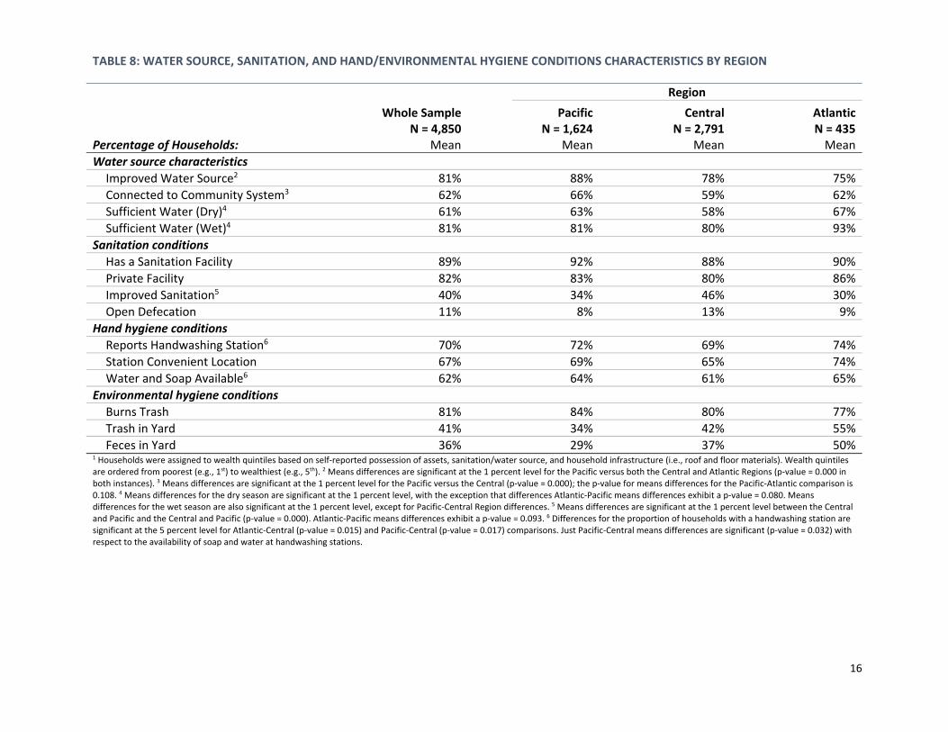
4.2 Water Source, Sanitation, and Hand/Environmental Hygiene Conditions

Table 8 presents descriptive statistics for water source, sanitation, hand hygiene, and environmental hygiene

characteristics among the evaluation sample. 81% of all households in the sample have an improved water source,

23 with 62% of households connected to a community water system. Households in the Pacific Region exhibit higher

proportions of households with an improved water source24 and connected to a community system25 (88% and 66%,

respectively) in comparison to households in the Central (78% and 59%) and Atlantic (75% and 62%) (Figure 4). 89%

of all sample households have a sanitation facility; however, just 40% have improved sanitation as defined by the

Joint Monitoring Programme (JMP).26 The Central Region exhibits the highest level of improved sanitation of the

three regions (46% versus 34% and 30% in the Pacific and Atlantic Regions, respectively).27 Open defecation is also

the highest in the Central Region (13%) in comparison to the Pacific (8%) and Atlantic (9%).

23 The definition for improved water source is based on that of the WHO/UNICEF (2015) Joint Monitoring Programme for Water Supply and Sanitation (JMP). Improved water sources include (i) systems connected to the community water system; (ii) protected springs; (iii) protected wells; and (iv) rainwater harvesting systems. 24 Means differences are significant at the 1 percent level for the Pacific versus both the Central and Atlantic Regions (p‐value of 0.000 in both instances). 25 Means differences are significant at the 1 percent level for the Pacific versus the Central (p‐value of 0.000); Pacific‐Atlantic means differences exhibit a p‐value of 0.108. 26 The definition for improved sanitation is based on that of the WHO/UNICEF (2015) Joint Monitoring Programme for Water Supply and Sanitation (JMP). Improved sanitation includes (i) a flush toilet that empties into a sewer, septic tank, or pit; (ii) a ventilated improved pit (VIP) latrine; and (iii) an ecological dry latrine. 27 Means differences are significant at the 1 percent level between the Central and Pacific (p‐value of 0.000). Atlantic‐Pacific means differences exhibit a p‐value of 0.093.

11%

24%

29%

14%

24%

19%17%

22%

18%

24%

18% 18%

35%

12%

16%

0%

5%

10%

15%

20%

25%

30%

35%

40%

Pacific Central Atlantic

Figure 3. Distribution of Households by Household Wealth Quintile and Region

1st 2nd 3rd 4th 5th

16

TABLE 8: WATER SOURCE, SANITATION, AND HAND/ENVIRONMENTAL HYGIENE CONDITIONS CHARACTERISTICS BY REGION

Region


Pacific N = 1,624

Central N = 2,791

Atlantic N = 435

Percentage of Households: Mean Mean Mean Mean

Water source characteristics

Improved Water Source2 81% 88% 78% 75%

Connected to Community System3 62% 66% 59% 62%

Sufficient Water (Dry)4 61% 63% 58% 67%

Sufficient Water (Wet)4 81% 81% 80% 93%

Sanitation conditions

Has a Sanitation Facility 89% 92% 88% 90%

Private Facility 82% 83% 80% 86%

Improved Sanitation5 40% 34% 46% 30%

Open Defecation 11% 8% 13% 9%

Hand hygiene conditions

Reports Handwashing Station6 70% 72% 69% 74%

Station Convenient Location 67% 69% 65% 74%

Water and Soap Available6 62% 64% 61% 65%

Environmental hygiene conditions

Burns Trash 81% 84% 80% 77%

Trash in Yard 41% 34% 42% 55%

Feces in Yard 36% 29% 37% 50% 1 Households were assigned to wealth quintiles based on self‐reported possession of assets, sanitation/water source, and household infrastructure (i.e., roof and floor materials). Wealth quintiles are ordered from poorest (e.g., 1st) to wealthiest (e.g., 5th). 2 Means differences are significant at the 1 percent level for the Pacific versus both the Central and Atlantic Regions (p‐value = 0.000 in both instances). 3 Means differences are significant at the 1 percent level for the Pacific versus the Central (p‐value = 0.000); the p‐value for means differences for the Pacific‐Atlantic comparison is 0.108. 4 Means differences for the dry season are significant at the 1 percent level, with the exception that differences Atlantic‐Pacific means differences exhibit a p‐value = 0.080. Means differences for the wet season are also significant at the 1 percent level, except for Pacific‐Central Region differences. 5 Means differences are significant at the 1 percent level between the Central and Pacific and the Central and Pacific (p‐value = 0.000). Atlantic‐Pacific means differences exhibit a p‐value = 0.093. 6 Differences for the proportion of households with a handwashing station are significant at the 5 percent level for Atlantic‐Central (p‐value = 0.015) and Pacific‐Central (p‐value = 0.017) comparisons. Just Pacific‐Central means differences are significant (p‐value = 0.032) with respect to the availability of soap and water at handwashing stations.

17


Households were asked whether they have sufficient water to attend to their daily water needs (i.e. bathing, washing

clothing, preparing food) in the wet and dry seasons, respectively. Overall, 81% of households report having

sufficient water in the wet season compared to just 61% in the dry season. Households in the Atlantic region report

having sufficient water in the wet and dry seasons with greater frequency than households in either the Pacific or

Central regions.28

With respect to household hygiene characteristics, 70% of households in the sample have a space for washing hands

and 62% a handwashing station with soap and water.29 In total, 41% of households have trash in their yards, while

36% have feces in their yards. Atlantic households were the most likely to have a handwashing station; however,

they were also the most likely to have feces in their yard (50%, Table 8).30

Table 9 breaks out water source, sanitation, and hand and environmental hygiene conditions by household wealth

quintile. Trends in access to an improved water source, the frequency of a community water connection, as well as

the possession of an improved sanitation facility and a handwashing station with soap and water are consistent with

what would be expected: coverage increase among higher wealth quintile. For instance, more than 90% of

households in the top wealth quintile have access to an improved water source, relative to just 62% of households

in the poorest wealth quintile. Wealthier households are also twice as likely to be connected to a community water

system than households in the poorest wealth quintile and trend toward having sufficient water in the wet and dry

seasons with greater frequency. Households in the wealthiest quintile are almost twice as likely to report having

improved sanitation, as well as a washing station with soap and water, compared to households in the poorest

wealth quintile; poorer households are significantly more likely to report practicing open defecation (30% of

households in the bottom wealth quintile compared to 2% of households in the top wealth quintile). The likelihood

of having trash and feces in a household’s yard decreases with increases in household wealth.

28 Means differences for the dry season are significant at the 1 percent level, with the exception that differences between the Atlantic and Pacific coasts exhibit a p‐value of 0.080. Means differences for the wet season are also significant at the 1 percent level, with the exception of Pacific‐Central Region differences. 29 Differences for the proportion of households with a handwashing station are significant at the 5 percent level for Atlantic‐Central (p‐value of 0.015) and Pacific‐Central (p‐value of 0.017) comparisons. Just Pacific‐Central means differences are significant (p‐value of 0.032) with respect to the availability of soap and water at handwashing stations. Differences are significant at the 5 percent level for Pacific‐Central differences in the availability of water and soap at wash stations and not significant in the case of Atlantic‐Central differences. 30 The surveyor observed (1) whether there was a hand‐washing station and (2) recorded whether or not there was soap and water at said station. He or she also observed the front yard and noted whether he or she saw feces and/or trash.

88%

66%

34%

78%

59%

46%

75%

62%

30%

0%

20%

40%

60%

80%

100%

Improved Water Source Connected to CommunitySystem

Improved Sanitation

Figure 4. Proportion of HH with improved water sources and improved sanitation, by region

PacificN = 1,624

CentralN = 2,791

AtlanticN = 435

18

TABLE 9: WATER SOURCE, SANITATION, AND HAND/ENVIRONMENTAL HYGIENE CONDITIONS CHARACTERISTICS BY HOUSEHOLD WEALTH QUINTILE



1st

N = 970

2nd

N = 972

3rd

N = 968

4th

N = 970

5th

N = 970 Percentage of Households: Mean Mean Mean Mean Mean Mean

Water source characteristics

Improved Water Source 81% 62% 78% 83% 88% 94%

Connected to Community System

62% 39% 58% 61% 71% 80%

Sufficient Water (Dry) 61% 55% 58% 61% 64% 66%

Sufficient Water (Wet) 81% 78% 81% 82% 83% 84%

Sanitation conditions

Has a Sanitation Facility 89% 71% 89% 94% 95% 98%

Private Facility 82% 65% 80% 86% 87% 91%

Improved Sanitation 40% 29% 38% 39% 42% 53%

Open Defecation 11% 30% 10% 7% 4% 2%

Hand hygiene conditions

Reports Handwashing Station 70% 52% 66% 71% 77% 87%

Station Convenient Location 67% 49% 63% 67% 74% 84%

Water and Soap Available 62% 46% 58% 61% 68% 80%

Environmental hygiene conditions

Burns Trash 81% 83% 82% 82% 84% 73%

Trash in Yard 41% 49% 41% 44% 38% 32%

Feces in Yard 36% 47% 39% 38% 33% 21% 1 Households were assigned to wealth quintiles based on self‐reported possession of assets, sanitation/water source, and household infrastructure (i.e., roof and floor materials). Wealth quintiles are ordered from poorest (e.g., 1st) to wealthiest (e.g., 5th).

19

4.3 General Household Characteristics

This section reviews a range of household socio‐demographic characteristics, including household socio‐

demographic characteristics, head of household education level and participation in economic activities. Table 10

exhibits descriptive statistics of socio‐demographic characteristics for households in the sample. At the top, there is

a breakdown of individuals in different age brackets across household wealth quintiles. Thereafter, descriptive

statistics for household size are displayed, with 4.7 family members in the average household. There do not appear

to be many differences in household age profile or household size across wealth quintiles. On average, household

heads are 46 years old and male in 54% of households. Broadly, the proportion of male household heads decreases

with increases in household wealth.

Table 11 shows descriptive statistics for household heads in the sample. Overall, 3% of household heads self‐identify

as indigenous, with a higher proportion of poor households led by individuals identifying as indigenous compared to

wealthier households. With respect to economic activity, 81% of household heads report active employment with

73% reporting income from economic activities during the last month. Frequencies of active employment, income

in the last month, and income from employment are relatively homogenous across wealth quintiles, with the

exception that household heads in the top wealth quintile report having income during the prior month with greater

frequency than the first four wealth quintiles (88% versus 83% overall). Table 11 also indicates that a large

percentage of household heads have attended school and are literate, at 69% and 70%, respectively. However, just

44% of household heads have completed their primary education, and 12% their secondary education. When broken

out by wealth quintile, the relationship between poverty and education, or a lack thereof, becomes clear with

households in the bottom wealth quintile more than 2.5 times more likely to not have attended any primary school

than households in the top wealth quintile (53% versus 21%). Similar patterns are found with respect to completion

of primary, secondary, and post‐secondary school with wealthier household heads more likely to have completed

higher levels of education.

4.4 Water Source and Safe Water‐Use Behavior

Baseline data collection included several questions about the source of water for households and the extent of

household water treatment activities. Descriptive statistics for these variables are exhibited in Table 12. 62% of

households in the IE sample have a system connection and the same percentage of all households collected their

last drink of water from the community system. Additionally, a significant majority of households took their last drink

of water from a storage container inside of their home (84%) compared to just 14% of households taking their last

drink of water directly from the tap; drinking water quality deteriorates during storage in the household and

consumption of stored water is considered a risk factor for waterborne diseases (Wright et al., 2004; Trevett et al.,

2004; Clasen and Bastable, 2003). Just 24% of households reported treating their last drink of water – 20% reported

treating their water through chlorination. 51% of these households did not treat their water because they did not

believe it was necessary, either because someone had told them so or because their local CAPS had told them that

water had already been treated. Wealthier households are more likely to report treating their water than less

wealthy households, with 28% of households in the highest wealth quintile having treated water and just 17% of

households in the lowest wealth quintile having done so. Confirmation of chlorination through household water

samples was rare: only 3 in 29 samples taken from storage containers in households that reported treating drinking

water present in the household were positive for chlorine, and only 1 of 29 samples taken from household taps

connected to systems that reported treating water with chlorine tested positive for the presence of chlorine (data

not shown).31

Table 13 shows descriptive statistics for the extent to which households said that they had enough water to attend

to their daily water needs. 82% of households with a water connection stated that they had enough water in the wet

31 In the case of the tap samples, the sample with a positive chlorine reading was positive for free chlorine; no tap samples were positive for residual chlorine.

20

TABLE 10: SOCIO‐DEMOGRAPHIC CHARACTERISTICS OF THE HOUSEHOLD BY HOUSEHOLD WEALTH QUINTILE


Whole Sample

N = 4,850

1st

N = 970

2nd

N = 972

3rd

N = 968

4th

N = 970

5th

N = 970

Mean Mean Mean Mean Mean Mean

% of sample

HH members, 5 and under 13% 3% 3% 2% 3% 2%

HH members, 6‐13 17% 4% 4% 4% 3% 3%

HH members, 14‐30 34% 6% 7% 7% 7% 7%

HH members, 31‐65 31% 5% 6% 6% 6% 7%

HH members 65+ 5% 1% 1% 1% 1% 1%

All ages 100% 20% 20% 20% 20% 20%

Number of household members

Average HH size 4.7 4.58 4.74 4.76 4.72 4.69

HH members, 5 and under 0.60 0.65 0.61 0.58 0.62 0.55

HH members, 6‐13 .82 .88 .87 .83 .78 .76

HH members, 14‐30 1.58 1.52 1.61 1.62 1.59 1.57

HH members, 31‐65 1.46 1.26 1.41 1.47 1.53 1.61

HH members 65+ 0.25 0.29 0.27 0.27 0.22 0.2

Household size

1 3% 4% 2% 3% 2% 2%

2 9% 10% 8% 8% 9% 9%

3 19% 20% 21% 19% 19% 18%

4 23% 23% 22% 22% 22% 24%

5 18% 16% 17% 18% 20% 20%

6 12% 11% 13% 12% 12% 12%

7 7% 6% 6% 8% 7% 7%

8+ 10% 10% 11% 10% 10% 8%

Household head

Average age, HH head 46.39 46.56 46.46 47.2 46.12 45.63

HH heads, % male 54% 56% 58% 55% 53% 48% 1 Households were assigned to wealth quintiles based on self‐reported possession of assets, sanitation/water source, and household infrastructure (i.e., roof and floor materials). Wealth quintiles are ordered from poorest (e.g., 1st) to wealthiest (e.g., 5th).

21

TABLE 11: DISTRIBUTION OF HOUSEHOLD HEAD DEMOGRAPHIC AND EDUCATION CHARACTERISTICS BY HOUSEHOLD WEALTH QUINTILE



1st

N = 970

2nd

N = 972

3rd

N = 968

4th

N = 970

5th

N = 970

% of household heads: Obs. Mean Mean Mean Mean Mean Mean

Identifies as Indigenous 4,437 3% 5% 3% 2% 2% 3%

Reports Active Employment 4,850 81% 82% 80% 79% 80% 82%

Any Income Prior Month 4,842 83% 81% 82% 82% 82% 88%

Income from Employment 4,842 73% 73% 71% 71% 73% 76%

Education

No Primary 4,846 37% 53% 43% 39% 29% 21%

Primary 4,846 44% 37% 43% 45% 46% 47%

Secondary 4,846 12% 6% 7% 10% 15% 20%

Post‐Secondary 4,846 3% 1% 2% 2% 5% 8%

Is literate 4,850 70% 53% 65% 68% 78% 86%

Ever attended school 4,846 69% 52% 63% 67% 78% 86% 1 Households were assigned to wealth quintiles based on self‐reported possession of assets, sanitation/water source, and household infrastructure (i.e., roof and floor materials). Wealth quintiles are ordered from poorest (e.g., 1st) to wealthiest (e.g., 5th).

22

TABLE 12: DISTRIBUTION OF HOUSEHOLD WATER SOURCE CHARACTERISTICS BY HOUSEHOLD WEALTH QUINTILE


Whole Sample

N = 4,850

1st N = 970

2nd N = 972

3rd N = 968

4th

N = 970

5th N = 970

% of Households: Mean Mean Mean Mean Mean Mean Water source characteristics

Connected to Comm. System 62% 39% 58% 61% 71% 80%

Last drink of water Source: Comm. System 62% 42% 59% 62% 71% 76% Collected: from tap 14% 9% 10% 14% 18% 19% Collected: from storage 84% 91% 89% 85% 80% 76% Treated 24% 17% 23% 24% 25% 28% Treated chlorination 20% 14% 19% 21% 22% 23%

Treatment not necessary2 51% 49% 51% 48% 54% 55%

1 Households were assigned to wealth quintiles based on self‐reported possession of assets, sanitation/water source, and household infrastructure (i.e., roof and floor materials). Wealth quintiles are ordered from poorest (e.g., 1st) to wealthiest (e.g., 5th). 2 “Treatment not necessary” is a binary variable for which households were assigned a 1 if they did not treat water because they did not think treatment was necessary, someone told them that it was not necessary, or their CAPS told them that it was already treated.

TABLE 13: SUFFICIENCY OF WATER SUPPLY BY SYSTEM CONNECTION STATUS AND HOUSEHOLD WEALTH QUARTILE


Whole Sample

N = 4,850

1st N = 970

2nd N = 972

3rd N = 968

4th N = 970

5th N = 970

Percentage of Households: Mean Mean Mean Mean Mean Mean

Sufficient Water: Dry With a system 66% 63% 64% 64% 67% 69% Without a system 53% 50% 51% 56% 54% 54%

Sufficient Water: Wet With a system 82% 80% 80% 81% 83% 83%

Without a system 81% 76% 83% 83% 85% 87% 1 Households were assigned to wealth quintiles based on self‐reported possession of assets, sanitation/water source, and household infrastructure (i.e., roof and floor materials). Wealth quintiles are ordered from poorest (e.g., 1st) to wealthiest (e.g., 5th).

23

season compared to 81% without a connection. During the dry season 66% of households with a system connection

report having enough water relative to just 53% of households without a connection. In both the wet and dry

seasons, wealthier households respond that they have sufficient water with greater frequency than poorer

households.

Table 14 shows descriptive statistics for continuity of water service for connected households in the wet and dry

seasons. As expected, households have more hours of service in the water‐abundant wet season than during the dry

season, averaging 15.2 and 13.3 hours, respectively. Regional break‐outs show that the Atlantic has more hours of

service in both the wet and dry seasons, followed by the Central and Pacific regions. There is a significant amount of

variance in service level both across wealth quintiles and regions, with a broad trend towards increased service levels

among lower wealth quintiles. Sixty‐two percent and 48 percent of households state that they experience daily or

weekly service interruptions during the dry and wet seasons, respectively. Similar to the trend in hours of service,

wealthier households tend to experience service interruptions with greater frequency than the poor. Wealthier

households also reported using more water than poorer households, consuming 241 liters of water per capita

compared to an average of 186 liters across all quintiles, and an average of 154 liters for households in the bottom

wealth quintile. Wealthier households also spend more on water, with households in the wealthiest quintile

spending just shy of 3 times as much on water as households in the bottom wealth quintile on a per‐month basis.

4.5 Waterborne Illness Prevalence

Tables 15 through 17 present descriptive statistics on diarrhea prevalence, disaggregated by age. Overall, 9% and

7% of households have had family members with diarrhea symptoms in the last week and 2 days, respectively.

Similarly, 7% children under the age of 5 have had diarrhea symptoms in the last week. Diarrhea prevalence is the

highest in the Pacific and the Atlantic, 10% in both regions, and 8% in the Central Region (Table 15). There does not

seem to be a strong relationship between reported diarrhea prevalence and household wealth, with no clear trend

in diarrhea prevalence across wealth quintiles (Table 16). Diarrhea prevalence segmented by whether households

have improved sanitation, a water connection, and soap and water available at a handwashing station is displayed

in Table 17. Having improved sanitation and a water connection are both related to a decreased prevalence of

diarrhea. Households with soap and water reported higher levels of diarrhea prevalence. A limitation of the baseline

survey is that temporality could not be assessed between hygiene practices and the presence of soap and water; it

is possible that households with existing cases of diarrhea were more likely to be practicing proper hand hygiene, as

opposed to soap and water being the cause of diarrhea.

4.6 Community Characteristics

Table 18 displays characteristics for the 300 communities at baseline, using data collected from the community

survey. For Table 18, as well as other tables displaying information across wealth quintiles for community, system,

CAPS, and UMAS data, household wealth scores were averaged across the communities, systems, CAPS or UMAS –

yielding average wealth scores aggregated to the unit of interest. Aggregate wealth scores were used to classify units

(e.g. community, system) into one of the five wealth quintile categories based on the quintile cutoffs established for

the household distribution.

Average community size was 115 households, with a positive relationship between the average household wealth

quintile of a community and the number of households in that community. In relation to WSS infrastructure, 86% of

communities have improved sanitation and 97% of communities are covered by at least one water system (data not

shown).32 In contrast, most communities in the sample have less than 50% coverage of improved sanitation. Overall,

wealthier communities tend to have access to improved sanitation more frequently than poorer communities.

Wealthier communities are also more likely to report having sufficient water throughout the entire year, with 85%

The community survey included questions on whether a community had electricity, fixed and mobile phone

32 Just 8 communities in our baseline data have no community water system.

24

TABLE 14: DISTRIBUTION OF HOUSEHOLD WATER USE CHARACTERISTICS BY HOUSEHOLD WEALTH QUINTILE



1st

N = 970

2nd

N = 972

3rd

N = 968

4th

N = 970

5th

N = 970

% of Households: Obs. Mean Mean Mean Mean Mean Mean Water Use

Sufficient Water (Dry) 4,850 61% 55% 58% 61% 64% 66% Sufficient Water (Wet) 4,850 81% 78% 81% 82% 83% 84% Hours of service per day (Dry) 2,990 13.27 14.8 13.35 13.42 13.47 12.2

Pacific 1,076 11.57 12.78 11.28 11.73 12.62 10.69 Central 1,643 13.67 14.15 13.43 13.58 13.42 14.05 Atlantic 271 17.61 20.71 17.33 19.17 17.56 14.47

Hours of service per day (Wet) 2,990 15.21 17.62 15.56 15.63 15.29 13.42 Pacific 1,076 12.93 15.28 13.08 14.15 13.63 11.58 Central 1,643 15.93 17.35 15.76 15.72 15.94 15.18 Atlantic 271 19.94 22.3 19.6 21.17 19.21 18.31

Difference in Hours (Wet – Dry)2 2,981 2.11 2.92 2.24 2.25 1.82 1.34

Service interruptions (Dry)3 2,990 62% 56% 61% 63% 61% 65%

Service interruption (Wet)3 2,990 48% 40% 48% 49% 47% 53% Monthly payment (NIO) 2,737 74.45 39.43 46.96 58.35 81.57 112.18

Amount of water used (Liters) 4,850 185.52 154.32 154.02 179.51 199.08 240.72

Amount of time to retrieve water (minutes)

4,797 8.18 8.83 7.98 8.16 7.53 8.4

Who Manages Household Water?

Female Member 4,797 86% 86% 84% 85% 87% 88% 1 Households were assigned to wealth quintiles based on self‐reported possession of assets, sanitation/water source, and household infrastructure (i.e., roof and floor materials). Wealth quintiles are ordered from poorest (e.g., 1st) to wealthiest (e.g., 5th). 2 Difference in Hours (Wet – Dry) represents the total difference in hours of service for households by subtracting the number of hours of service in the dry season from the number of service hours in the wet season. 3 Service interruptions for the wet and dry seasons is a binary variable for which households were assigned a 1 if they said that they experienced daily or weekly interruptions in water service in the wet and dry seasons and a 0 if they did not.

25

TABLE 15: DISTRIBUTION OF DIARRHEA PREVALENCE BY REGION

Region


Pacific N = 1,624

Central N = 2,791

Atlantic N = 435

Percentage of Households: Obs. Mean Mean Mean Mean

Any family member

Symptoms in the last week 4,850 8.7% 10.1% 7.7% 9.9%

Symptoms in the last 2 days 4,850 6.8% 7.6% 6.2% 7.4%

Child less than five years old

Symptoms in the last week 2,183 6.9% 7.7% 6.4% 7.8%

TABLE 16: DISTRIBUTION OF DIARRHEA PREVALENCE BY HOUSEHOLD WEALTH QUINTILE



1st

N = 970

2nd

N = 972

3rd

N = 968

4th

N = 970

5th

N = 970

% of Households: Obs. Mean Mean Mean Mean Mean Mean

Any family member

Symptoms in the last week 4,850 8.7% 7.5% 9.9% 7.7% 10.7% 7.7%

Symptoms in the last 2 days 4,850 6.8% 6.2% 8% 6.5% 7.5% 5.6%

Child less than five years old

Symptoms in the last week 2,183 6.9% 4.8% 9.9% 5.4% 7.4% 7.1% 1 Households were assigned to wealth quintiles based on self‐reported possession of assets, sanitation/water source, and household infrastructure (i.e., roof and floor materials). Wealth quintiles are ordered from poorest (e.g., 1st) to wealthiest (e.g., 5th).

26

TABLE 17: DISTRIBUTION OF DIARRHEA PREVALENCE1 BY WATER, SANITATION, AND HYGIENE CONDITIONS

Improved Sanitation Water Connection Soap and Water

Percentage of HHs with: No Yes No Yes No Yes

Any family member

Symptoms in last week 9.0% 8.3% 9.3% 8.4% 7.8% 9.3%

Symptoms in last 2 days 7.2% 6.2% 7.9% 6.6% 5.8% 7.3% **

Children

Symptoms in last week 7.2% 6.6% 7.3% 6.5% 5.2% 8.0% *** 1 Respondents were asked whether someone living in the household had diarrhea in the last week and in the last two days. They were asked to identify the number of households in each age range experiencing diarrhea symptoms. *** Statistically significant at the 1 percent level, ** Statistically significant at the 5 percent level

27

TABLE 18: COMMUNITY‐LEVEL CHARACTERISTICS BY QUINTILE OF AVERAGE HOUSEHOLD WEALTH SCORE

Quintile of Average Household Wealth Score1

Whole Sample N = 300

1st

N = 18

2nd

N = 82

3rd

N = 100

4th

N = 73

5th

N = 26 Obs. Mean Mean Mean Mean Mean Mean

General community characteristics

No. HH 294 115 43 90 103 144 208

Indigenous community 294 7% 12% 7% 8% 3% 8%

Has improved sanitation 283 86% 82% 77% 84% 94% 96%

>50% HH have improved sanitation 300 49% 44% 40% 54% 60% 31%

Community has sufficient water 290 63% 53% 59% 56% 74% 85%

Community infrastructure

Has electricity 294 69% 18% 25% 84% 99% 100%

Has fixed phone lines 294 7% 0% 1% 3% 14% 27%

Has cell phone connection 294 89% 94% 84% 88% 93% 96%

Has internet 294 17% 6% 6% 13% 28% 42%

No. Water Systems

0 291 3% 6% 1% 4% 1% 4%

1 291 74% 38% 72% 75% 79% 85%

2 291 12% 19% 11% 12% 13% 8%

3 291 6% 25% 9% 3% 4% 0%

School characteristics

Has a school 294 93% 94% 93% 96% 93% 85%

Has a school with water connection 274 79% 56% 68% 80% 88% 100%

Has a school with improved sanitation 274 66% 50% 75% 61% 68% 68%

Health post characteristics

Community has a health post 294 22% 0% 12% 21% 34% 42%

Community has a health post with water connection

294 19% 0% 7% 17% 30% 42%

Community has a health post with improved sanitation

294 16% 0% 7% 13% 24% 38%

Hands washed 293 20% 0% 10% 20% 30% 38%

Handwashing station with soap and water 291 14% 0% 5% 15% 17% 35%

Household Hygiene Practices

>50% HH have hand‐washing station >10m of toilet

280 43% 13% 33% 45% 49% 58%

. . . with water and soap 276 36% 33% 27% 33% 46% 42% 1 Households were assigned to wealth quintiles based on self‐reported possession of assets, sanitation/water source, and household infrastructure (i.e., roof and floor materials). Wealth quintiles are ordered from poorest (e.g., 1st) to wealthiest (e.g., 5th). Household wealth scores were then averaged across communities, after which each community was assigned to a wealth quintile based on thresholds utilized to group households into wealth quintiles. Wealth quintiles are ordered from poorest (e.g., 1st) to wealthiest (e.g., 5th).

28

infrastructure, and internet. In general, 69% of communities have electricity, with electrification more common in

wealthier communities. Cell phone infrastructure is the only infrastructure category in which all communities have

relatively high coverage. 93% of communities have a school, while significantly fewer communities (22%) have a

health post. Wealthier communities are more likely to have schools and health posts with water system connections

and improved sanitation. For instance, no communities in the lowest wealth quintile have a health post, in

comparison with 42% of communities in the top wealth quintile.

In addition to community infrastructure characteristics, the community survey included several questions about

household water hygiene. In just 43% and 36% of communities do more than half of all households have a

handwashing station and a handwashing station with soap and water within 10 meters from the toilet, respectively.

4.7 Water System Characteristics

Of principal importance in data collection were questions related to water systems and CAPS. Table 19 shows

descriptive statistics for the 316 systems in the sample, by the quintile of the average household wealth quintile for

system‐users.33

It should be noted that even though several communities had more than three systems, a decision was made during

data collection to limit the number of systems for which system‐level data was collected to three given resource and

time constraints. Systems for which data was collected are an average of 12.4 years old and cover an average of 76

users. Systems in wealthier communities cover more users and a higher percentage of potential users. Gravity fed

systems were the most frequent (47% of systems). Pumped systems are more frequent among systems at the top

two wealth quintiles.

The average system draws from 1.4 sources. More than half of a system’s sources have sufficient water for 91% and

69% of systems in the wet and dry seasons, respectively. Respondents were asked about the condition of key WSS

system infrastructure components. At least one of the water system’s sources are reported to be in poor condition

for 21% of systems, and at least one source was reported to be contaminated by garbage/sewage and chemicals for

22% in both cases. 35% of systems of systems reported having at least one un‐protected source. Systems serving

wealthier households tended to draw from better quality and better protected sources.

Just 26% of systems were reported to have treatment infrastructure, with a strong relationship between the wealth

level of households served by a system and the existence of treatment infrastructure. Respondents for 33% of

systems claimed that water was treated with chlorination with only 10% having applied chlorination in the last 10

days. However, chlorination analyses conducted in the field detected positive levels of total chlorination in just four

of 15 instances, and residual chlorination in just two cases where chlorination was reported in the previous 10 days

(data not shown). Almost 78% of systems have distribution infrastructure, 8% of which a component of the

distribution infrastructure was reported to be in poor condition. 71% of systems were reported to have storage

infrastructure, 15% of which reported having storage infrastructure in poor condition. Again, there is evidence of a

possible relationship between the relative wealth of households served by a system and the likelihood that

distribution and storage infrastructure is in poor condition.

4.8 Service Provider Characteristics

4.8.1 Institutional Strength

Much of the research on rural water system sustainability emphasizes the importance of the institutional aspects of

service providers in addition to water system infrastructure. In many contexts, like that of rural Nicaragua, water

33 Due to miscoding during data collection and entry, it was not possible to match households to water systems for 15 of 331 systems. Data for these systems are included in descriptive statistics shown for the entire sample, but not included in descriptive statistics shown for the quintile of the average household wealth score associated with systems.

29

TABLE 19: WATER SYSTEM CHARACTERISTICS BY QUINTILE OF AVERAGE HOUSEHOLD WEALTH SCORE


Whole Sample

N = 316

1st

N = 6

2nd

N = 53

3rd

N = 64

4th

N = 65

5th

N = 31

% of Systems: Obs. Mean Mean Mean Mean Mean Mean

Infrastructure

System age (years) 287 12.4 11.5 10.0 13.4 12.5 13.6

No. system users 223 76 24 38 50 108 187

% of HHs Connected to System 220 62% 64% 52% 60% 77% 78%

Water System Technology

Drilled Well 305 12% 0% 0% 2% 13% 6%

Dug Well 305 5% 0% 2% 0% 3% 3%

Pumped system 305 25% 0% 14% 11% 46% 65%

Manual well 305 11% 0% 0% 3% 0% 3%

Gravity system 305 47% 100% 84% 84% 38% 23%

Source Characteristics

No. sources 302 1.4 1.5 1.2 1.2 1.2 1.2

Sources have sufficient water: Dry2 300 69% 50% 71% 66% 75% 71%

Sources have sufficient water: Wet2 300 91% 100% 92% 95% 94% 87%

Any Source . . .

. . . in poor condition 251 21% 20% 19% 27% 7% 10%

. . . contaminated by garbage/sewage 297 22% 0% 22% 16% 16% 23%

. . . contaminated by chemicals 289 22% 20% 27% 26% 16% 23%

. . . not surrounded by green areas 294 14% 0% 6% 15% 14% 10%

. . . surrounded by eroded areas 289 23% 20% 20% 21% 29% 23%

. . . not protected 289 35% 40% 43% 32% 24% 29%

Treatment Characteristics

Has treatment infrastructure 303 26% 33% 24% 37% 33% 42%

Water treated with chlorine 298 33% 17% 27% 40% 41% 35%

Chlorine applied in last 15 days 303 10% 0% 8% 13% 13% 19%

Other Infrastructure Condition

Has distribution infrastructure 299 78% 83% 100% 94% 98% 100%

Any distr. Infra in poor condition 229 8% 0% 13% 14% 2% 6%

Has storage infrastructure 299 71% 83% 90% 90% 95% 90%

Any storage infra in poor condition 210 15% 20% 20% 22% 8% 7%

1 Households were assigned to wealth quintiles based on self‐reported possession of assets, sanitation/water source, and household infrastructure (i.e., roof and floor materials). Wealth quintiles are ordered from

poorest (e.g., 1st) to wealthiest (e.g., 5th). Household wealth scores were then averaged across water systems, after which each water system was assigned to a wealth quintile based on thresholds utilized to group households into wealth quintiles. Wealth quintiles are ordered from poorest (e.g., 1st) to wealthiest (e.g., 5th). 2 Sources have sufficient water is a binary variable for which systems for which more than half of sources were said by respondents to have sufficient water in a given season received a 1, while systems for which fewer than half of sources have sufficient water in a given season received a 0.

30

systems are frequently managed by local water boards with varying levels of institutionalism. A rich survey of CAPS

service providers was included in PROSASR baseline data collection to understand the extent to which institutional

capacity exists in the context of CAPS (Comité de Agua Potable y Saneamiento). Tables displaying descriptive

statistics for the 299 CAPS included in the baseline data are included in Tables 20‐24.34

Table 20 provides descriptive statistics for the education level of CAPS leadership.35 57% of CAPS presidents

completed primary school with 25% and 14% having completed secondary and a university education, respectively.

Similar to data on household head education, there is evidence of a relationship between community wealth level

and education level of CAPS leadership, with the highest level of education completed by a CAPS president increasing

with the wealth level of CAPS users. Table 21 provides data on the institutionalism, professionalism, and mechanisms

for community participation in CAPS. Overall, it appears that service providers serving wealthier households exhibit

higher levels of institutionalism. In total, just 35% of water committees are legalized; however, about half of CAPS in

the top two wealth quintiles are legal versus 0% and 28% in the bottom two wealth quintiles, respectively. CAPS in

wealthier areas also hold more meetings on average than those in poorer areas, with CAPS in the top wealth quintile

holding 3.5 meetings on average over the last six months versus 1.5 for CAPS in the bottom wealth quintile. 62% of

CAPS are fully‐elected. 37% of CAPS have women in leadership roles.

Increased professionalism of CAPS could allow service providers to respond quickly and effectively to technical

problems related to water systems. 67% and 44% of CAPS have technical and paid technical staff, respectively, with

systems in wealthier areas more likely to employ technical and paid technical staff than systems in less well‐off areas.

About half of all CAPS have complaint‐receiving mechanisms and are accountable to system users.36 Again, systems

serving wealthier households exhibit higher frequencies for community participation variables than systems serving

poorer households.

4.8.2 Financial Sustainability

In addition to institutional capacity, the literature highlights the importance of adequate financial management of

CAPS operations. The extent to which CAPS charge for their services, whether they cover costs, and how well they

manage funds, are detailed in Table 22. Overall, three‐quarters of CAPS have a monthly tariff with the monthly tariff

variable (tied to usage) for just 21% of service providers. Variable tariffs permit CAPS to charge users for the amount

of water they draw from the system, obliging users consuming more to pay more than those using less. An average

monthly tariff among tariff‐charging CAPS is USD 3.09; CAPS in the wealthiest quintile charge three‐times more, on

average, than CAPS in the second‐to‐last wealth quintile. On average, 72% of users are current on payments with

some evidence that poorer communities are more likely to experience delinquent payments. Approximately 40% of

CAPS cannot cover costs, indicating that CAPS may not be charging enough or that their financial management is

inefficient.

4.8.3 Operations & Management and Government Assistance

A third determinant of water system sustainability from the perspective of service providers has to do with the

extent to which CAPS perform maintenance and receive government assistance to do so. Systems receiving

preventative care may be less likely to break down. Corrective care would be necessary in the case of an

unanticipated system problem. Descriptive statistics for CAPS in the baseline data are exhibited in Table 23. 74% of

CAPS provide corrective care versus just 53% providing preventative care. Indeed, CAPS serving wealthier users are

34 Again, due to miscoding during data collection and data entry, CAPS were matched to the households they provide water service to for 223 of 299 CAPS for which data were collected at baseline. 35 Surveyors sought to identify the CAPS president, or other individual with knowledge of CAPS. The surveyor then asked about the highest level of education achieved by said individual. 36 “Accountable to users” is a dummy variable for which system providers were assigned a 1 if they report back to users at least once every six months and have meeting minutes to demonstrate it.

31

TABLE 20: EDUCATION LEVEL OF CAPS LEADERSHIP1 BY HOUSEHOLD WEALTH QUINTILE BY QUINTILE OF AVERAGE HOUSEHOLD WEALTH SCORE



1st

N = 6

2nd

N = 53

3rd

N = 65

4th

N = 67

5th

N = 33

% of CAPS: Obs. Mean Mean Mean Mean Mean Mean

Less than primary 269 5% 20% 9% 10% 2% 0%

Primary 269 57% 80% 65% 65% 48% 23%

Secondary 269 25% 0% 15% 16% 29% 45%

University 269 14% 0% 11% 10% 22% 32% 1 The survey firm was asked to locate the CAPS president or other individual with knowledge of the CAPS. The above table describes the distribution of the education level of these individuals. 2 Wealth scores were averaged across service providers, after which each service provider was assigned to a wealth quintile based on thresholds utilized to group households into wealth quintiles. Wealth quintiles are ordered from poorest (e.g., 1st) to wealthiest (e.g., 5th).

32

TABLE 21: INSTITUTIONALISM, PROFESSIONALISM AND PARTICIPATION CHARACTERISTICS OF CAPS BY QUINTILE OF AVERAGE HOUSEHOLD WEALTH SCORE



1st

N = 6

2nd

N = 53

3rd

N = 65

4th

N = 67

5th

N = 33


Institutionalism

Service Provider is a CAPS 276 70% 40% 74% 86% 84% 64%

CAPS age 165 6.8 3.0 7.5 7.6 5.8 7.4

CAPS legalized 276 35% 0% 28% 38% 52% 45%

CAPS fully‐elected 277 62% 20% 70% 84% 75% 58%

No. meetings last 6 months 184 2.8 1.5 2.9 2.8 3.2 3.5

No. CAPS committee members

240 5.4 5.4 5.5 6.0 5.4 5.6

% women in CAPS leadership

230 37% 26% 24% 32% 42% 47%

Professionalism

Has technical staff 258 67% 60% 67% 72% 81% 82%

Technical staff paid 257 44% 0% 36% 53% 57% 67%

Participation

Has complaint‐receiving mechanism

262 45% 20% 52% 58% 48% 67%

Accountable to users2 251 52% 0% 55% 71% 63% 58%

Women participate in meetings

258 89% 60% 84% 97% 98% 97%

1 Households were assigned to wealth quintiles based on self‐reported possession of assets, sanitation/water source, and household infrastructure (i.e., roof and floor materials). Wealth quintiles are ordered from poorest (e.g., 1st) to wealthiest (e.g., 5th). Household wealth scores were then averaged across CAPS, after which each CAPS was assigned to a wealth quintile based on thresholds utilized to group households into wealth quintiles. Wealth quintiles are ordered from poorest (e.g., 1st) to wealthiest (e.g., 5th). 2 “Accountable to users” is a binary variable for which system providers were assigned a 1 if they report back to users at least one every six months and have meeting minutes to prove it.

33

TABLE 22: FINANCIAL SUSTAINABILITY CHARACTERISTICS OF CAPS BY QUINTILE OF AVERAGE HOUSEHOLD WEALTH SCORE



1st

N = 6

2nd

N = 53

3rd

N = 65

4th

N = 67

5th

N = 33


Has monthly tariff 265 73% 60% 74% 87% 92% 94%

Monthly tariff is variable 265 21% 0% 9% 15% 47% 36%

Average monthly tariff (USD)

192 3.089 .242 2.293 3.078 2.403 6.372

% of HH current on payments

176 72% 47% 68% 66% 79% 70%

Accounting books to date 252 56% 20% 53% 70% 71% 72%

CAPS covers costs (e.g., solvent)

147 62% 100% 64% 68% 59% 52%

Has bank account 231 26% 0% 20% 16% 47% 37% 1 Households were assigned to wealth quintiles based on self‐reported possession of assets, sanitation/water source, and household infrastructure (i.e., roof and floor materials). Wealth quintiles are ordered from poorest (e.g., 1st) to wealthiest (e.g., 5th). Household wealth scores were then averaged across CAPS, after which each CAPS was assigned to a wealth quintile based on thresholds utilized to group households into wealth quintiles. Wealth quintiles are ordered from poorest (e.g., 1st) to wealthiest (e.g., 5th).

34

TABLE 23: SERVICE PROVIDER O&M AND GOVERNMENT ASSISTANCE CHARACTERISTICS OF CAPS BY QUINTILE OF AVERAGE HOUSEHOLD WEALTH SCORE



1st

N = 6

2nd

N = 53

3rd

N = 65

4th

N = 67

5th

N = 33


O&M

Provides preventative care 266 53% 20% 53% 65% 55% 81%

Provides corrective care 266 74% 100% 96% 90% 67% 78%

Has materials for O&M 260 46% 20% 47% 51% 54% 75%

Promotes environmental sanitation

267 81% 80% 83% 84% 87% 70%

Protects area around source 267 90% 100% 91% 95% 92% 88%

Government Assistance

Requested gov’t support 270 54% 40% 57% 47% 57% 61%

Requested and received government support

269 38% 40% 43% 35% 43% 48%

Requested, but did not receive government support

269 16% 0% 15% 11% 14% 12%

Reports problem to UMAS 261 36% 0% 37% 30% 37% 47%

UMAS responsive 261 24% 0% 20% 18% 32% 41% 1 Households were assigned to wealth quintiles based on self‐reported possession of assets, sanitation/water source, and household infrastructure (i.e., roof and floor materials). Wealth quintiles are ordered from poorest (e.g., 1st) to wealthiest (e.g., 5th). Household wealth scores were then averaged across CAPS, after which each CAPS was assigned to a wealth quintile based on thresholds utilized to group households into wealth quintiles. Wealth quintiles are ordered from poorest (e.g., 1st) to wealthiest (e.g., 5th).

35

more likely to apply preventative care, with CAPS in the top wealth quintile providing preventative care four times

more than CAPS in the bottom wealth quintile. There is a corresponding negative relationship with respect to

corrective care with CAPS in poorer wealth quintiles relying on corrective care more frequently than CAPS in

wealthier quintiles. Less than 50% of all CAPS have materials for providing maintenance. Nonetheless, 81% and 90%

of CAPS report promoting environmental sanitation and protecting areas around system sources, respectively,

actions that may enhance system sustainability of the system and quality of the water provided to households.

At the municipal level, UMAS are responsible for providing technical assistance to CAPS. They are frequently the

ones called upon by CAPS in the case of doubts or for technical and training needs. According to the survey, 54% of

CAPS requested government support; 38% requested and ultimately received assistance. 16% of CAPS reported

requesting, but did not receive support from UMAS. 36% of CAPS reported communicating system problems to

UMAS with UMAS responsive to 24%. There is some evidence that CAPS report service issues and that UMAS are

responsive more often for CAPS in wealthier areas than poorer areas.

4.8.4 Community Interaction with CAPS

The household survey included several questions to gauge the extent to which households interacted with CAPS

over the previous two months. CAPS engaging more frequently with community members may have an increased

ability to detect and respond faster to service and system problems than CAPS engaging to a lesser degree.

Additionally, they may have the social capital necessary to convince system users to pay tariffs on time, increasing

the likelihood that funds are available for timely preventative and corrective system care. Table 24 shows descriptive

statistics for household interaction with CAPS.

Overall, 55% of households had at least some contact with their local CAPS in the two months before the survey,

with contact higher for wealthier households than for the less well‐off. The most common types of contact are

attending a meeting (30%) and making a payment to CAPS (28%). Overall, females attended CAPS meetings more

frequently than males, although marginally.

When asked about the last time a household or someone in the community encountered an issue with water service,

about half of households said that a local CAPS resolved the service issue, with CAPS resolving the service issues of

wealthier households more frequently than for poor households. Higher relative rates of CAPS resolving water issues

may be related to increased relative institutional capacity. Finally, 13% of households reported that their community

had received a training by their CAPS in the last year.

4.9 Municipal WSS Units

In addition to household and system‐level surveys, baseline data were also collected at the municipal level (UMAS).

One of the objectives of the PROSASR initiative is building the institutional capacity of UMAS. It is expected that

intervention will encourage UMAS to provide better technical assistance to CAPS, improving the performance of

rural water systems and increasing the long‐term sustainability of systems. An UMAS survey was conducted for each

of the 77 municipalities in the baseline data; however, due to a coding errors one of the municipalities was unable

to be matched to household data. Table 25 displays descriptive statistics for the entire UMAS sample, as well as by

average household wealth quintile for the 76 UMAS successfully matched to households from the household survey.

Overall, each UMAS was responsible for an average of 54 communities. On average, UMAS reported that 44% of

communities solicit the support of UMAS and 41% of communities are ultimately attended to by UMAS. Consistent

with the level of institutional development of CAPS, communities in municipalities with wealthier households tend

to request and receive support from UMAS with increased frequency relative to poorer municipalities. Slightly less

than half of all UMAS are assigned funds from the municipal budget; budget support is reported to be sufficient for

supporting CAPS in just 20% of UMAS.

36

TABLE 24: DISTRIBUTION OF HOUSEHOLD INTERACTION WITH SERVICE PROVIDERS BY HOUSEHOLD WEALTH QUINTILE



1st

N = 970

2nd

N = 972

3rd

N = 968

4th

N = 970

5th

N = 970

Obs. Mean Mean Mean Mean Mean Mean

% of Households:

Community has CAPS 4,850 75% 65% 73% 73% 79% 86%

Contact with CAPS 4,844 55% 44% 52% 54% 61% 62%

Membership contact 4,844 6% 4% 6% 6% 7% 5%

Payment contact 4,844 28% 20% 24% 27% 34% 34%

Attended meeting contact 4,844 30% 27% 30% 28% 32% 31%

Woman attended CAPS meeting

4,849 17% 12% 14% 18% 20% 21%

Man attended CAPS meeting 4,849 15% 16% 17% 13% 15% 13%

Man and woman attended meeting

4,849 2% 2% 3% 2% 3% 3%

Knowledge of CAPS meeting 4,849 57% 47% 54% 57% 64% 65%

CAPS resolved last service problem

4,849 49% 35% 45% 47% 56% 60%

Time to resolve service problem (Days)

3,658 8.4 4.4 5.9 5.7 9.6 15.1

CAPS training in last year 4,849 13% 8% 12% 14% 16% 15% 1 Households were assigned to wealth quintiles based on self‐reported possession of assets, sanitation/water source, and household infrastructure (i.e., roof and floor materials). Wealth quintiles are ordered from poorest (e.g., 1st) to wealthiest (e.g., 5th).

37

TABLE 25: MUNICIPAL TECHNICAL ASSISTANCE PROVIDER (UMAS) CHARACTERISTICS BY QUINTILE OF AVERAGE HOUSEHOLD WEALTH SCORE


Whole Sample

N = 77

1st

N = 1

2nd

N = 18

3rd

N = 27

4th

N = 27

5th

N = 3

% of UMAS Obs. Mean Mean Mean Mean Mean Mean

No. communities assigned to UMAS 76 53.8 26.0 55.7 68.8 43.7 16.7

% communities soliciting support 76 44% 35% 35% 44% 47% 55%

% of communities attended 76 41% 23% 29% 40% 46% 80%

Annual budget assigned to UMAS 76 47% 0% 33% 50% 48% 100%

% Budget / Total Budget 30 26% .% 4% 24% 46% 0%

Budget sufficient for CAPS support 35 20% .% 20% 15% 31% 0%

Has own transportation 76 61% 0% 72% 69% 44% 67%

Has water‐quality measurement equip. 76 42% 0% 50% 54% 30% 33%

Has IT equipment 76 74% 0% 83% 81% 59% 100%

Budgeted travel expenses 76 54% 0% 61% 62% 37% 100%

Budgeted gasoline 76 66% 0% 67% 69% 59% 100%

More nat. government training needed 75 76% 100% 67% 80% 74% 100%

Received training from FISE/ARAS 77 87% 100% 83% 78% 100% 67% 1 Households were assigned to wealth quintiles based on self‐reported possession of assets, sanitation/water source, and household infrastructure (i.e., roof and floor materials). Wealth quintiles are

ordered from poorest (e.g., 1st) to wealthiest (e.g., 5th). Household wealth scores were then averaged across UMAS, after which each UMAS was assigned to a wealth quintile based on thresholds

utilized to group households into wealth quintiles. Wealth quintiles are ordered from poorest (e.g., 1st) to wealthiest (e.g., 5th).

38

The UMAS survey asked about the extent to which UMAS had equipment on hand for CAPS support. Even though

61% of UMAS have their own transportation and 74% have their own information technology equipment, just 42%

of UMAS have equipment to measure water quality.

Lastly, UMAS were asked about the extent to which they would like to receive more training, alluding to the Results‐

Oriented Learning AVAR‐component of PROSASR. 76% of UMAS responded that more training was necessary from

the national government. 67 of the 77 UMAS, or 87% in the baseline data had received at least one training

intervention from the national government.

4.10 Water Quality

4.10.1 Household Samples

Water quality tests were conducted at different points throughout water systems. Results for samples taken at the

household level are exhibited in Table 26. Analyses were conducted for 373 households in 146 communities and for

147 systems. 335 samples were taken from a storage container in the household and 171 from household taps.

When duplicate samples were taken in households and the results differed (n = 5) average E. coli MPN was preserved

for analysis. Mean E. coli MPN for storage samples across all households (regardless of the source from which the

last glass of water was taken) was 24.1 MPN (“high risk”).37 Mean E. coli MPN across all tap samples was 21.5 (also

“high risk”). To further assess differences between tap and storage water quality, controlling for other household

factors, we utilized paired tap‐storage samples from the 121 households for which paired samples were available.

On average, paired storage samples were more contaminated than tap samples (Tap: 16.8 E. coli MPN; Storage: 23.1

E. coli MPN, mean difference 6.2 E. coli MPN), with means differences significant at the 1 percent level (p‐value =

0.001). Table 26 also shows E. coli MPN for households based on the source from which their last drink was taken.

On average, the E. coli MPN for storage samples for households taking their last glass from the storage container

was 25.3 MPN. For households taking their last glass from the tap, E. coli MPN for tap samples was 18.0.

Table 27 exhibits the distribution of household samples by contamination risk category. The risk level of water taken

from storage containers and from the tap is “safe” in 27% and 26% of households, respectively. Water was absent

of E. coli contamination in 25% of households from the last glass sample was taken from a storage container,

compared to 31% of households for which the last glass was taken from the tap.

4.10.2 System Samples

At the system level, E. coli samples were taken from storage tanks, and from system sources. 307 samples were

taken for 169 systems, with 24 samples dropped from the dataset due to miscoding during data entry. After dropping

miscoded samples, there are data for 141 system sources and 89 system tank samples. In the 18 cases for which

more than one sample was taken for a given system‐source or system‐tank combination, mean E. coli MPN was kept

for the purposes of descriptive statistics and subsequent analyses.

Table 28 shows E. coli MPN at the system level for source, tank, tap, and storage container samples, as well as for

paired source‐tank, tank‐tap, tap‐storage, and source‐storage samples. Overall, average E. coli MPN tell a story of

deteriorating water quality as water moves from source to a household storage container. Mean E. coli MPN for

Systems at the source is 19.5, corresponding to a “high” water quality risk. Mean E. coli MPN for system storage is

10.6, possibly indicative of reductions in E. coli MPN associated with settling in the tank, or indicator die off (Levy et

al., 2008). Alternatively, the reduction in E. coli MPN from source to storage could be explained by treatment by

CAPS; however, this seems unlikely given the very low frequency of confirmed chlorination in the field. From there,

water quality deteriorates significantly with average E. coli MPN at the tap and storage 23.5 and 22.7, respectively.

Also displayed in Table 28 are differences in E. coli MPN between different points in water systems for systems in

37 An MPN cap of 101 was placed on E. coli MPN detectable by water quality analyses.

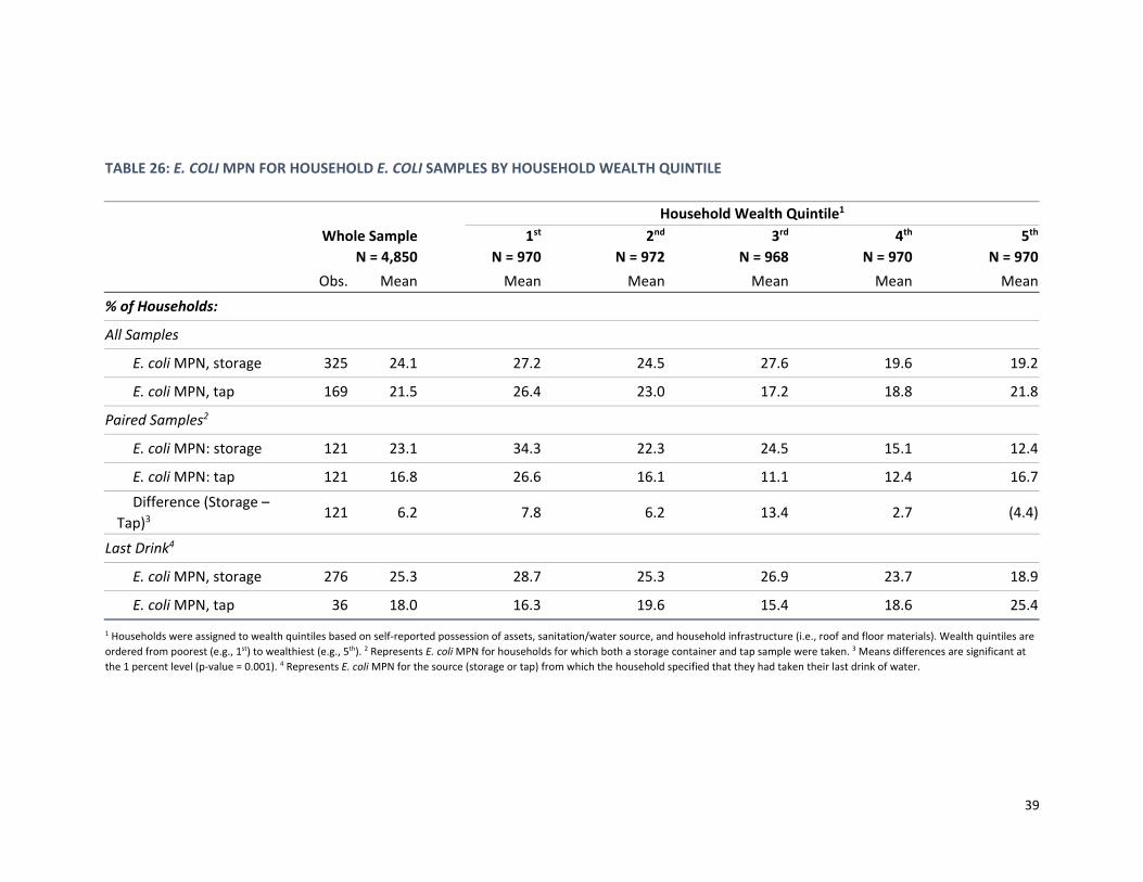
39

TABLE 26: E. COLI MPN FOR HOUSEHOLD E. COLI SAMPLES BY HOUSEHOLD WEALTH QUINTILE


Whole Sample

N = 4,850

1st

N = 970

2nd

N = 972

3rd

N = 968

4th

N = 970

5th

N = 970


% of Households:

All Samples

E. coli MPN, storage 325 24.1 27.2 24.5 27.6 19.6 19.2

E. coli MPN, tap 169 21.5 26.4 23.0 17.2 18.8 21.8

Paired Samples2

E. coli MPN: storage 121 23.1 34.3 22.3 24.5 15.1 12.4

E. coli MPN: tap 121 16.8 26.6 16.1 11.1 12.4 16.7

Difference (Storage –

Tap)3 121 6.2 7.8 6.2 13.4 2.7 (4.4)

Last Drink4

E. coli MPN, storage 276 25.3 28.7 25.3 26.9 23.7 18.9

E. coli MPN, tap 36 18.0 16.3 19.6 15.4 18.6 25.4

1 Households were assigned to wealth quintiles based on self‐reported possession of assets, sanitation/water source, and household infrastructure (i.e., roof and floor materials). Wealth quintiles are

ordered from poorest (e.g., 1st) to wealthiest (e.g., 5th). 2 Represents E. coli MPN for households for which both a storage container and tap sample were taken. 3 Means differences are significant at

the 1 percent level (p‐value = 0.001). 4 Represents E. coli MPN for the source (storage or tap) from which the household specified that they had taken their last drink of water.

40

TABLE 27: E. COLI RISK LEVELS FOR SAMPLES – SOURCE, TANK, TAP, AND STORAGE SAMPLES1

Risk Level2

% of samples: Safe Inter. High Very High

Source (N = 139) 59% 17% 6% 17%

Tank (N = 89) 58% 25% 10% 7%

Tap (N = 169) 26% 38% 22% 14%

Storage (N = 325) 27% 33% 30% 10%

Last Drink

Tap (N = 36) 31% 36% 25% 8%

Storage (N = 276) 25% 33% 32% 10% 1 Descriptive statistics for tap, storage, and last drink samples shown at the household level; statistics for source and tank samples shown at the system level. 2 Risk categories correspond to the following E. coli MPN: Safe (0), Intermediate (1 to 10), High (10 to 100), Very High (100 and above).

41

TABLE 28: SYSTEM‐LEVEL E. COLI MPN1 AND MPN DIFFERENCES BY QUINTILE OF AVERAGE HOUSEHOLD WEALTH SCORE2



1st N = 6

2nd N = 53

3rd N = 69

4th N = 71

5th N = 35


E. coli MPN: source 139 19.5 3.5 33.0 13.3 19.2 20.2

E. coli MPN: tank 89 10.6 0.8 12.9 12.7 9.4 10.2

E. coli MPN: tap 82 23.5 2.0 23.6 23.0 27.9 12.4

E. coli MPN: storage 139 22.7 12.4 29.7 26.2 15.6 18.9

Differences (Paired Samples Only)

Tank ‐ Source 60 ‐3.7 ‐1.1 ‐9.9 8.4 ‐10.9 0.0

Tap – Tank** 63 7.0 . 5.6 4.1 9.2 1.4

Storage ‐ Tap 75 ‐0.2 6.6 9.8 5.5 ‐13.0 ‐5.4

Storage – Source** 108 7.2 12.8 1.9 19.8 4.3 1.4 1 E. coli MPN represents average MPN for a system, averaged across all systems for which E. coli analyses were conducted. 2 Risk categories correspond to the following E. coli MPN: Safe (0), Intermediate (1 to 10), High (10 to 100), Very High (100 and above). 3 Households were assigned to wealth quintiles based on self‐reported possession of assets, sanitation/water source, and household infrastructure (i.e., roof and floor materials). Wealth quintiles are ordered from poorest (e.g., 1st) to wealthiest (e.g., 5th). Household wealth scores were then averaged across water systems, after which each water system was assigned to a wealth quintile based on thresholds utilized to group households into wealth quintiles. Wealth quintiles are ordered from poorest (e.g., 1st) to wealthiest (e.g., 5th). *** Statistically significant at the 1 percent level, ** Statistically significant at the 5 percent level

42

which paired source‐tank, tank‐tap, and tap‐storage samples exist. The greatest one‐step difference (i.e., source to

tank represents one step, while source to tap represents two steps) in water quality is between tank and tap samples,

with a gap of 7.0 E. coli MPN, with means differences statistically significant at the 5 percent level (p‐value = 0.05).

The difference in water quality from source to storage containers is 7.2 E. coli MPN, on average. Mean differences

are also significant at the 5 percent level (p‐value = 0.037). Paired storage‐tap differences are negligible.

While more than half of source and tank samples are classified as safe (Table 27), there is a clear deterioration of

water quality as it makes its way through the system. In the regressions displayed in Section 6, we explore the

determinants “safe” water quality at the system level.

5. Baseline Balance Check

In order for the results of a randomized control to be valid, the treatment and control groups must be exchangeable

with respect to observable and unobservable characteristics that could potentially impact the outcomes of interest.

To assess the effectiveness of randomization at creating balanced treatment arms we evaluated the balance of

measured baseline characteristics. Tables 29‐36 present baseline balance checks for key household, community,

system, and CAPS characteristics. The validity of the design relies on randomization to provide overall balance across

treatment arms; however, we also conducted tests for differences in means for specific variables and report resulting

test statistics, accordingly.

The results of balance checks suggest that treatment and control group households are relatively well‐balanced,

increasing the likelihood that we will be able to detect the impacts of the PROSASR intervention with respect to key

final and intermediate outcome variables, consistent with the initial IE design.

Overall, 176 variables are presented in the aforementioned tables. Across all characteristics there is evidence of

good balance between treatment and control arms. Key outcome variables, such as the proportion of households

with access to an improved water source and improved sanitation, as well as indicators of the sustainable operation

of CAPS, appear balanced, suggesting equivalence between treatment arms. Similarly, there are no significant

differences in most demographic, socio‐economic, and water use characteristics across treatment and control

households.

While treatment arms are well balanced overall, we note differences in specific characteristics that might be

important to account for in follow‐up analyses. Specifically, control households appear more likely to report their

last drink came from the tap, while treatment households are more likely to have taken their last drink from a storage

container (Table 30). Control households are also more likely to experience daily or weekly service disruptions in the

wet season relative to households in the treatment group (Table 30). Results from the community survey suggest

communities in the control group are more likely to report having sufficient water all year long compared to

treatment communities. Control group communities are also more likely to have a health post in the community

(Table 32). The average E. coli MPN for tap samples among treatment households taking their last glass of water

from the tap was higher than for control group households; though these estimates are based on a relatively small

sample (Table 35). To account for potential differences between treatment groups at baseline, these characteristics

will be controlled for in the follow‐up analyses to assess whether they impact the interpretation of results.

6. Correlates of Continuity of Water Service and Water Quality

This section discusses the implications of bivariate regressions exploring the correlates of water service continuity

and water quality. These analyses are purely informative and exploratory; no interpretation of causal link should be

drawn between the independent variables included in our analysis and the dependent variables we attempt to

explain. However, utilizing baseline data from the IE can offer some insight into factors that may contribute to water

system sustainability; these analyses could offer insight to PROSASR going forward.

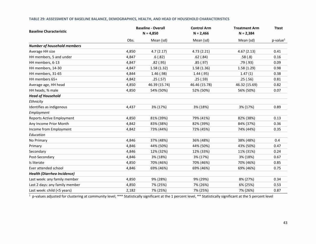
43

TABLE 29: ASSESSMENT OF BASELINE BALANCE, DEMOGRAPHICS, HEALTH, AND HEAD OF HOUSEHOLD CHARACTERISTICS

Baseline Characteristic Baseline ‐ Overall

N = 4,850

Control Arm

N = 2,466

Treatment Arm

N = 2,384

Ttest

Obs. Mean (sd) Mean (sd) Mean (sd) p‐value1

Number of household members

Average HH size 4,850 4.7 (2.17) 4.73 (2.21) 4.67 (2.13) 0.41

HH members, 5 and under 4,847 .6 (.82) .62 (.84) .58 (.8) 0.16

HH members, 6‐13 4,847 .82 (.95) .85 (.97) .79 (.93) 0.09

HH members, 14‐30 4,847 1.58 (1.32) 1.58 (1.36) 1.58 (1.29) 0.98

HH members, 31‐65 4,844 1.46 (.98) 1.44 (.95) 1.47 (1) 0.38

HH members 65+ 4,842 .25 (.57) .25 (.59) .25 (.56) 0.81

Average age, HH head 4,850 46.39 (15.74) 46.46 (15.78) 46.32 (15.69) 0.82

HH heads, % male 4,850 54% (50%) 52% (50%) 56% (50%) 0.07

Head of Household

Ethnicity

Identifies as indigenous 4,437 3% (17%) 3% (18%) 3% (17%) 0.89

Employment

Reports Active Employment 4,850 81% (39%) 79% (41%) 82% (38%) 0.13

Any Income Prior Month 4,842 83% (38%) 82% (39%) 84% (37%) 0.36

Income from Employment 4,842 73% (44%) 72% (45%) 74% (44%) 0.35

Education

No Primary 4,846 37% (48%) 36% (48%) 38% (48%) 0.4

Primary 4,846 44% (50%) 44% (50%) 43% (50%) 0.47

Secondary 4,846 12% (32%) 12% (33%) 11% (31%) 0.24

Post‐Secondary 4,846 3% (18%) 3% (17%) 3% (18%) 0.67

Is literate 4,850 70% (46%) 70% (46%) 70% (46%) 0.85

Ever attended school 4,846 69% (46%) 69% (46%) 69% (46%) 0.75

Health (Diarrhea Incidence)

Last week: any family member 4,850 9% (28%) 9% (29%) 8% (27%) 0.34

Last 2 days: any family member 4,850 7% (25%) 7% (26%) 6% (25%) 0.53

Last week: child (<5 years) 2,182 7% (25%) 7% (25%) 7% (26%) 0.87

1 p‐values adjusted for clustering at community level; *** Statistically significant at the 1 percent level, ** Statistically significant at the 5 percent level

44



N = 4,850

Control Arm N = 2,466

Treatment Arm

N = 2,384 Ttest

Obs. Mean (sd) Mean (sd) Mean (sd) p‐value1 Water

Source Characteristics

Improved Water Source 4,850 81% (39%) 80% (40%) 82% (39%) 0.71

Connected to Community System 4,844 62% (49%) 64% (48%) 60% (49%) 0.39

Sufficient Water (Dry Season) 4,850 61% (49%) 61% (49%) 61% (49%) 0.95

Sufficient Water (Wet Season) 4,850 81% (39%) 80% (40%) 83% (38%) 0.27

Last Drink of Water

Last Drink Source: Community System 4,797 62% (49%) 64% (48%) 59% (49%) 0.31

Last Drink Direct from Tap 4,850 14% (35%) 16% (37%) 12% (33%) 0.09

Last Drink from Storage Container 4,850 84% (36%) 82% (38%) 87% (34%) 0.05 **

Last Drink Treated 4,797 24% (42%) 23% (42%) 24% (43%) 0.53

Last Drink Treated with Chlorine 4,797 20% (40%) 18% (39%) 21% (41%) 0.19

Water Use

Believe treatment is Not Necessary 4,797 51% (50%) 52% (50%) 50% (50%) 0.51

Hours of service per day (Dry Season) 2,990 13.27 (10.13) 12.71 (10.13) 13.9 (10.09) 0.37

Hours of service per day (Wet Season) 2,990 15.21 (10) 14.26 (10.13) 16.27 (9.74) 0.13

Difference (Wet ‐ Dry) 2,981 2 (5.45) 1.65 (4.73) 2.38 (6.12) 0.19

Service interruption (Dry) 2,990 62% (49%) 65% (48%) 59% (49%) 0.25

Service interruption (Wet) 2,990 48% (50%) 54% (50%) 42% (49%) 0.02 **

Monthly payment (córdobas) 2,737 74.45 (92.06) 81.4 (92.25) 66.82 (91.29) 0.13

Amount of water used (Liters) 4,850 185.52 (164.11) 185.14 (163.96) 185.91 (164.29) 0.94

Amount of time to retrieve water 4,797 8.18 (29.03) 8.42 (35.37) 7.92 (20.59) 0.76

Who Manages Household Water?

Female Member 4,797 86% (35%) 87% (34%) 85% (36%) 0.17

Sanitation

Has Sanitation Facility 4,849 89% (31%) 90% (30%) 89% (31%) 0.48

Private Facility 4,849 82% (39%) 82% (38%) 82% (39%) 0.89

Improved Sanitation 4,849 40% (49%) 39% (49%) 42% (49%) 0.45

Open defecation 4,849 11% (31%) 10% (30%) 11% (31%) 0.59

Hand Hygiene

Reports Handwashing Station 4,850 70% (46%) 71% (46%) 70% (46%) 0.9

Station Convenient Location 4,849 67% (47%) 68% (47%) 67% (47%) 0.85

Water and Soap Available 4,849 62% (48%) 63% (48%) 62% (49%) 0.81

Environmental Hygiene

Trash in Yard 4,849 41% (49%) 39% (49%) 42% (49%) 0.43

Feces in Yard 4,849 36% (48%) 33% (47%) 38% (49%) 0.11


45



N = 4,850

Control Arm

N = 2,466

Treatment

Arm N = 2,384

Ttest

Mean (sd) Mean (sd) Mean (sd) p‐value1

Assets

Radio 60% (49%) 60% (49%) 60% (49%) 0.92

Television 64% (48%) 64% (48%) 64% (48%) 1

Refrigerator 25% (43%) 26% (44%) 24% (43%) 0.34

Iron 34% (47%) 34% (47%) 33% (47%) 0.81

Grinding Machine 35% (48%) 34% (48%) 35% (48%) 0.83

Cassette Recorder 6% (24%) 6% (24%) 6% (24%) 0.73

Stereo 20% (40%) 20% (40%) 19% (39%) 0.7

Fan 21% (41%) 22% (42%) 20% (40%) 0.49

Blender 17% (38%) 17% (38%) 17% (37%) 0.77

Sewing Machine 7% (25%) 7% (26%) 6% (24%) 0.17

Bicycle 28% (45%) 29% (45%) 27% (44%) 0.49

Motorcycle 14% (35%) 15% (35%) 14% (34%) 0.49

CD Player/DVD Player 19% (39%) 20% (40%) 18% (39%) 0.45

Cell Phone 65% (48%) 65% (48%) 66% (47%) 0.61

Computer 2% (15%) 2% (14%) 2% (15%) 0.66

Wealth Quintile

Poorest Quintile 20% (40%) 20% (40%) 20% (40%) 0.89

Second Wealth Quintile 20% (40%) 19% (39%) 21% (41%) 0.37

Third Wealth Quintile 20% (40%) 18% (39%) 22% (41%) 0.05 **

Fourth Wealth Quintile 20% (40%) 21% (41%) 19% (39%) 0.34

Richest Quintile 20% (40%) 21% (41%) 19% (39%) 0.35

Infrastructure

Floor Material

Concrete/tile 42% (49%) 43% (50%) 40% (49%) 0.39

Wood 3% (16%) 2% (15%) 3% (17%) 0.51

Earth/dirt 56% (50%) 55% (50%) 57% (50%) 0.49

Roof Material

Zinc sheet 88% (32%) 88% (33%) 88% (32%) 0.89

Tiled 10% (30%) 10% (30%) 10% (30%) 0.88

Fiberglass/asbestos 1% (9%) 1% (10%) 1% (9%) 0.89

Palm or non‐permanent 1% (10%) 1% (10%) 1% (10%) 0.84


46

TABLE 32: ASSESSMENT OF BASELINE BALANCE, WATER, SANITATION, AND HYGIENE: COMMUNITY SURVEY


N = 300

Control Arm

N = 150

Treatment Arm

N = 150 Ttest


General community characteristics

No. HH 294 115.2 (121.06) 116.48 (105.55) 113.93 (135.15) 0.86

No. systems 291 3.23 (15.6) 4.97 (22.03) 1.52 (1.49) 0.06

No. systems: 1 291 74% (44%) 75% (43%) 73% (45%) 0.67

No. systems: 2 291 12% (33%) 13% (34%) 11% (31%) 0.55

No. systems: 3 291 6% (23%) 3% (18%) 8% (27%) 0.09

Indigenous community 294 7% (25%) 7% (26%) 6% (24%) 0.64

Has improved sanitation 283 86% (35%) 83% (38%) 88% (33%) 0.23

>50% of HH have improved sanitation 300 49% (50%) 46% (50%) 53% (50%) 0.25

Water‐related epidemic in community 294 35% (48%) 33% (47%) 37% (49%) 0.47

% of communities with waste collected/treated 290 61% (49%) 62% (49%) 61% (49%) 0.86

% of communities with sufficient water 290 63% (48%) 71% (46%) 56% (50%) 0.01 ***

School characteristics

Has a school 294 93% (25%) 92% (27%) 95% (23%) 0.36

Has a school with water connection 274 79% (41%) 79% (41%) 78% (41%) 0.87

Has a school with improved sanitation 274 66% (47%) 67% (47%) 66% (47%) 0.93

Good hand washing practices taught 271 95% (22%) 93% (25%) 96% (19%) 0.24

Adequate water manipulation practices taught 268 93% (25%) 92% (28%) 95% (22%) 0.27

School bathroom has handwashing station w/soap and water 271 37% (48%) 35% (48%) 39% (49%) 0.5

Health post characteristics

Community has a health post 294 22% (42%) 29% (45%) 16% (37%) 0.01 ***

Community has a health post with a water connection 294 19% (39%) 24% (43%) 13% (34%) 0.01 ***

Community has a health post with improved sanitation 294 16% (36%) 19% (39%) 12% (33%) 0.11

Hands washed at health post 293 20% (40%) 25% (44%) 15% (36%) 0.03 **

Health post has handwashing station with soap and water 291 14% (34%) 15% (36%) 12% (33%) 0.45

Community infrastructure

Community has electricity 294 69% (46%) 69% (47%) 69% (47%) 1

Community has fixed phone lines 294 7% (26%) 8% (27%) 6% (24%) 0.5

Community has mobile phone connection 294 89% (31%) 90% (30%) 88% (32%) 0.71

Community has internet 294 17% (38%) 17% (38%) 17% (38%) 1

Household water use characteristics

>50% of HHs w/ hand‐washing station < 10m of latrine with water and soap 280 43% (50%) 41% (49%) 44% (50%) 0.62

>50% of HH have hand‐washing station < 10m of latrine/toilet 276 36% (48%) 33% (47%) 38% (49%) 0.41

>50% of HHs in which entire family using hand‐washing station 264 48% (50%) 45% (50%) 50% (50%) 0.45

>50% of HHs practicing safe water storage practices 281 86% (35%) 89% (32%) 83% (38%) 0.17

% of HH utilizing hygiene and water management practices 293 78% (41%) 79% (41%) 78% (42%) 0.86


47

TABLE 33: ASSESSMENT OF BASELINE BALANCE, WATER, SANITATION, AND HYGIENE: SYSTEM SURVEY

Baseline Characteristic

Baseline ‐ Overall N = 331

Control Arm

N = 159

Treatment Arm

N = 157 Ttest


Infrastructure

System age (Years) 287 12.4 (8.08) 12.37 (7.78) 12.44 (8.41) 0.94

No. system users 223 76.17 (110.19) 81.32 (98.88) 71.07 (120.59) 0.49

% of HHs connected to the system 220 62% (35%) 64% (35%) 60% (35%) 0.49

Drilled Well 305 12% (33%) 12% (33%) 13% (33%) 0.95

Dug Well 305 5% (21%) 6% (24%) 3% (18%) 0.29

Pumped system 305 25% (43%) 25% (44%) 24% (43%) 0.77

Manual well 305 11% (32%) 7% (26%) 16% (37%) 0.03 **

Gravity system 305 47% (50%) 49% (50%) 44% (50%) 0.39

Source characteristics

Number of sources 302 1.41 (1.11) 1.36 (.83) 1.47 (1.33) 0.43

Any source in poor condition 251 21% (41%) 19% (40%) 22% (42%) 0.6

Any source contaminated by garbage/sewage 297 22% (42%) 25% (44%) 19% (39%) 0.22

Any source contaminated by chemicals 289 22% (42%) 18% (39%) 26% (44%) 0.13

Any source not surrounded by green areas 294 14% (34%) 15% (36%) 12% (33%) 0.55

Any source surrounded by eroded areas 289 23% (42%) 21% (41%) 25% (44%) 0.36

Any source not protected 289 35% (48%) 35% (48%) 35% (48%) 1

Sources have sufficient water: summer 300 69% (46%) 72% (45%) 66% (47%) 0.26

Sources have sufficient water: winter 300 91% (28%) 89% (32%) 94% (24%) 0.11

Treatment characteristics

Treatment infrastructure exists 303 26% (44%) 23% (42%) 29% (45%) 0.23

Any treatment infra in poor condition 78 15% (36%) 17% (38%) 14% (35%) 0.71

Water treated with chlorine 298 33% (47%) 36% (48%) 29% (46%) 0.23

Receive assistance with chlorine treatment 108 46% (50%) 49% (50%) 43% (50%) 0.56

Residual chlorine analysis performed 120 20% (40%) 23% (42%) 17% (38%) 0.48

Chlorine applied in last 15 days 220 82% (39%) 83% (38%) 80% (40%) 0.6

Other infrastructure characteristics

Storage infrastructure exists 299 71% (46%) 73% (45%) 68% (47%) 0.43

Any storage infra in poor condition 210 15% (36%) 12% (33%) 19% (39%) 0.19

Distribution infrastructure exists 299 78% (41%) 79% (41%) 77% (42%) 0.61

Any distr. infra in poor condition 229 8% (28%) 8% (28%) 8% (27%) 0.92

No. public water intakes 296 1 (5.85) 1.26 (8.13) .74 (1.41) 0.44

>75% public water intakes >100m from HH 111 32% (47%) 25% (44%) 39% (49%) 0.12


48

TABLE 34: ASSESSMENT OF BASELINE BALANCE, WATER, SANITATION, AND HYGIENE: SERVICE PROVIDER SURVEY


N = 299

Control Arm

N = 150

Treatment Arm

N = 149 Ttest

Obs. Mean (sd) Mean (sd) Mean (sd) p‐value1 Institutionalism

Service Provider is a CAPS 276 70% (46%) 69% (46%) 71% (45%) 0.68

System age (Years) 287 12.4 (8.08) 12.37 (7.78) 12.44 (8.41) 0.94

CAPS is legalized 276 35% (48%) 33% (47%) 37% (48%) 0.49

CAPS fully‐elected 277 62% (49%) 60% (49%) 64% (48%) 0.45

No. meetings last 6 months 184 2.84 (2.68) 2.61 (2.42) 3.06 (2.91) 0.25

No. CAPS committee members 240 5.4 (1.7) 5.16 (1.83) 5.66 (1.52) 0.02 **

Women in CAPS leadership 230 37% (24%) 38% (24%) 36% (23%) 0.58

Professionalism

Has technical staff 258 67% (47%) 63% (48%) 72% (45%) 0.13

Technical staff is paid 257 44% (50%) 42% (49%) 46% (50%) 0.51

Participation

Has complaint mechanism 262 45% (50%) 41% (49%) 49% (50%) 0.18

Has accountability mechanism 251 52% (50%) 48% (50%) 56% (50%) 0.19

Women speak in meetings 258 89% (31%) 87% (34%) 92% (28%) 0.22

Finances

Has tariff 265 73% (44%) 71% (45%) 75% (43%) 0.47

Tariff is variable 265 21% (41%) 20% (40%) 22% (41%) 0.79

Average monthly tariff (USD) 192 3.09 (10) 2.92 (9.48) 3.24 (10.49) 0.82

% HH on time with payment 176 .72 (.27) .71 (.27) .72 (.28) 0.86

Accounting books to date 252 56% (50%) 51% (50%) 62% (49%) 0.07

Solvent 147 62% (49%) 61% (49%) 62% (49%) 0.91

Has savings account 231 26% (44%) 23% (42%) 29% (46%) 0.25

O&M and government assistance

Provides preventative care 266 53% (50%) 51% (50%) 55% (50%) 0.55

Provides corrective care 266 74% (44%) 77% (42%) 72% (45%) 0.33

Has materials for O&M 260 46% (50%) 42% (50%) 50% (50%) 0.22

Requested government support 270 54% (50%) 57% (50%) 52% (50%) 0.47

Requested and received government support 269 38% (49%) 35% (48%) 41% (49%) 0.31

Requested, did not receive government support 269 16% (37%) 21% (41%) 11% (32%) 0.02 **

Reports problems to UMAS 261 36% (48%) 34% (48%) 38% (49%) 0.52

UMAS responsive 261 24% (43%) 26% (44%) 22% (42%) 0.54

CAPS promotion activities

Promotes environmental sanitation 267 81% (39%) 84% (36%) 78% (42%) 0.18

Protects area around water source 267 90% (31%) 92% (27%) 87% (34%) 0.21 1 p‐values adjusted for clustering at community level; *** Statistically significant at the 1 percent level, ** Statistically significant at the 5 percent level

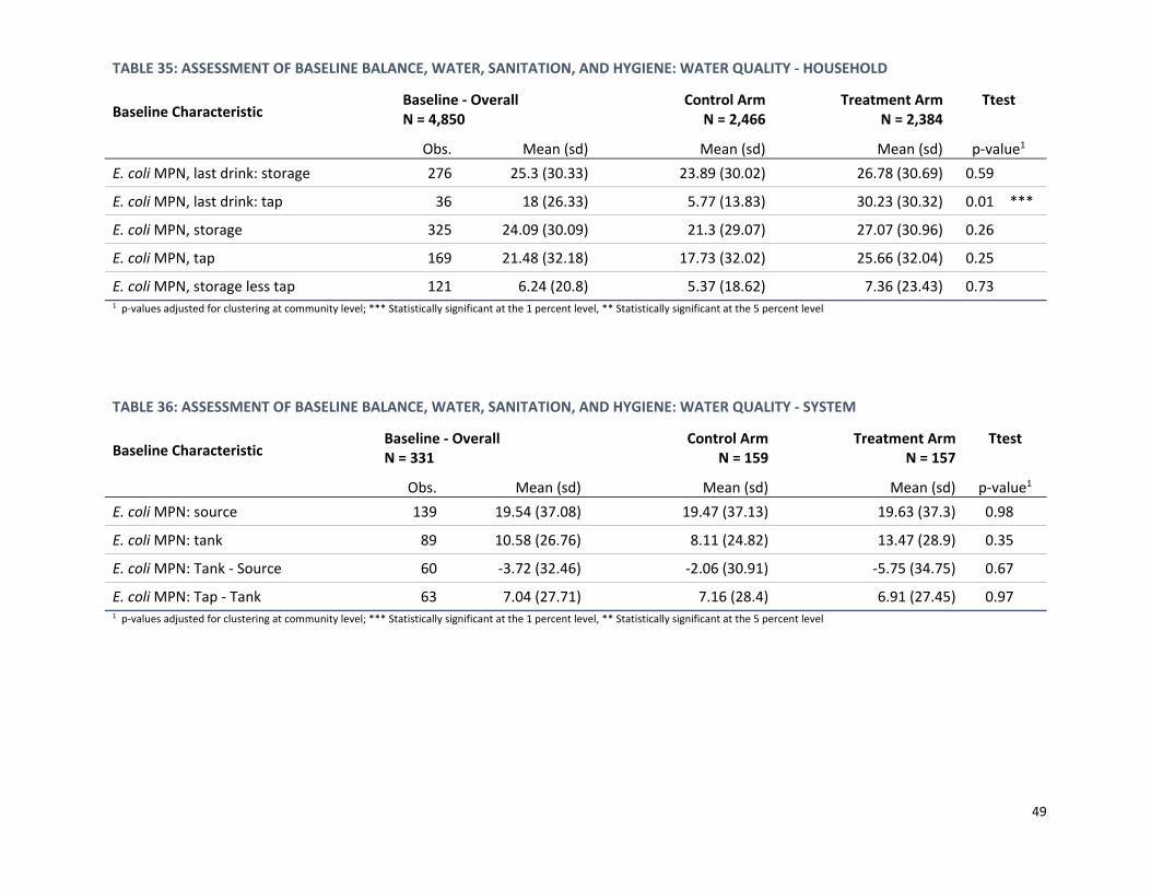
49

TABLE 35: ASSESSMENT OF BASELINE BALANCE, WATER, SANITATION, AND HYGIENE: WATER QUALITY ‐ HOUSEHOLD

Baseline Characteristic Baseline ‐ Overall N = 4,850

Control Arm

N = 2,466

Treatment Arm

N = 2,384 Ttest


E. coli MPN, last drink: storage 276 25.3 (30.33) 23.89 (30.02) 26.78 (30.69) 0.59

E. coli MPN, last drink: tap 36 18 (26.33) 5.77 (13.83) 30.23 (30.32) 0.01 ***

E. coli MPN, storage 325 24.09 (30.09) 21.3 (29.07) 27.07 (30.96) 0.26

E. coli MPN, tap 169 21.48 (32.18) 17.73 (32.02) 25.66 (32.04) 0.25

E. coli MPN, storage less tap 121 6.24 (20.8) 5.37 (18.62) 7.36 (23.43) 0.73 1 p‐values adjusted for clustering at community level; *** Statistically significant at the 1 percent level, ** Statistically significant at the 5 percent level

TABLE 36: ASSESSMENT OF BASELINE BALANCE, WATER, SANITATION, AND HYGIENE: WATER QUALITY ‐ SYSTEM

Baseline Characteristic Baseline ‐ Overall N = 331

Control Arm

N = 159

Treatment Arm

N = 157 Ttest


E. coli MPN: source 139 19.54 (37.08) 19.47 (37.13) 19.63 (37.3) 0.98

E. coli MPN: tank 89 10.58 (26.76) 8.11 (24.82) 13.47 (28.9) 0.35

E. coli MPN: Tank ‐ Source 60 ‐3.72 (32.46) ‐2.06 (30.91) ‐5.75 (34.75) 0.67

E. coli MPN: Tap ‐ Tank 63 7.04 (27.71) 7.16 (28.4) 6.91 (27.45) 0.97 1 p‐values adjusted for clustering at community level; *** Statistically significant at the 1 percent level, ** Statistically significant at the 5 percent level

50

6.1 Methodology

Given the need for evidence on the factors contributing to water system sustainability, we dedicate much of our

analysis to the correlates of water system continuity and microbial contamination. We use the average reported

number of hours of water service per day for households during the dry season as a proxy for water system

continuity. For each system, we averaged the reported number of hours of water service per day in the dry season

for all households connected to that system. For this analysis, data were available for 233 of the 316 systems (73.7%).

Next, we investigate the correlates of water quality at the system and household levels. We consider two measures

of water quality: (i) E. coli MPN and (ii) a binary variable for “safe water” (= 1 if 0 E. coli MPN per 100‐mL of water

were detected; = 0 if 1 or more E. coli MPN were detected in the sample). The first set of bivariate regressions

investigates system‐specific characteristics as correlates of household water quality. Water quality at the system

level, in this context, is gauged by averaging across all household tap samples linked to a given system.38 We

considered water quality at the tap as representative of the impact of the system on water quality before water is

handled by system end‐users in the household.

At the household level, we look at the water quality of household storage container samples. Storage container

samples offer insight into the quality of water once it has been handled by the end user, and is influenced by

household practices. In situations in which more than one storage container sample was taken, a household is

assigned the average E. coli MPN across all of that household’s samples. A second analysis was conducted using a

binary variable for safe water (= 1 if 0 E. coli MPN per 100‐mL of water were detected; = 0 if 1 or more E. coli MPN

were detected in the sample).

For water system continuity and quality at the system level, our independent variables of interest include water

system and CAPS characteristics. System‐level independent variables of interest include binary variables for the

following:

a. water system type (pumped versus gravity systems)

b. whether any water system source is:

i. contaminated by garbage or sewage

ii. contaminated by chemicals

iii. not surrounded by a green area

iv. surrounded by an eroded area

v. not protected

vi. in poor condition

c. whether a water system has:

i. treatment infrastructure

ii. storage infrastructure

iii. distribution infrastructure

d. whether any treatment, storage, and distribution infrastructure is in poor condition for systems with

associated treatment, storage, and distribution infrastructure.

For all binary variables other than water system type, a system was assigned a 1 in the case of an affirmative instance

(e.g., a system was contaminated with chemicals) and a 0 in the case of a negative instance (e.g., a system was not

contaminated by chemicals). System‐level variables were chosen based on the likelihood of their impacting water

quality and/or water service continuity. The rational for creating binary variables based on whether any component

is in poor condition or contaminated, not protected, etc. is that any water system weakness, regardless of the

magnitude, may have an adverse impact on water quality and/or water service continuity.

38 In cases in which more than one tap sample was taken for a given household, the value assigned to that household, for the purpose of this analysis, is the average of all tap samples associated with that household.

51

CAPS variables were taken into consideration to measure the extent to which the relative strength or weakness of a

local CAPS impacts the quality and continuity of the associated water system’s water. Variables proxying the level of

administrative and fiscal strength, as well as the level of service provided to water systems were incorporated into

bivariate regressions. Binary variables for whether the CAPS associated with a system fit the following criteria were

taken into consideration:

a. is legalized

b. has professional staff

c. has a verified complaint mechanism in place

d. is accountable to system users

e. charges a variable tariff

f. has accounting books that are to date

g. provides preventative care to water systems

h. applies a chlorination treatment and confirms that it works

i. applied a chlorination treatment in the 15 days preceding the survey

j. has received assistance from a municipal or national government entity

In addition to water system and CAPS variables, we look at means differences by (i) the quintile of the average

household wealth score for systems and (ii) region, utilizing Pacific, Central, and Atlantic region binary variables.

Given the richness of the household survey and the fact that storage container E. coli samples were taken during

data collection, we incorporate a series of bivariate regressions to investigate the correlates of water quality at the

household level. For bivariate regressions, we used binary variables for the characteristics of household water

source, household head characteristics, several proxies of wealth, as well as behaviors related to water and

sanitation. The specific binary variables we utilize for our analysis include the following:

a. Whether the household:

i. has an improved water source

ii. is connected to community system

iii. claims to have treated their last drink through chlorination

iv. practices open defecation

b. Whether the household head:

i. has studied some secondary school or more

ii. that manages the household’s water is female

iii. that manages the household’s water is female and has some secondary school or more

c. Household physical infrastructure characteristics

i. Floor type (firm versus earth)

ii. Roof type (zinc versus tiled/fiberglass/palm)

d. Whether the enumerator observed:

i. feces in the yard

ii. a handwashing station

iii. a handwashing station in a convenient location

iv. water and soap at the handwashing station

e. Whether the container used to store water had a wide mouth (e.g., one’s hand can fit into it) rather than a

small mouth.

Regional and household wealth quintile binary variables were also included in household water quality bivariate

regressions.

6.2 Results

This section summarizes findings for the correlates of water service levels and water quality based on bivariate

regressions. For each table, the independent variable of interest is found in the first column and is followed by the

52

number of observations and the mean for the two binary variable comparison groups (e.g., “does not have variable”

and “has variable”). The p‐value for means differences is found in the final column. Means differences significant at

the 1 and 5 percent levels are highlighted with three and two asterisks, respectively.

6.2.1 System‐Level Water Service

Table 37 exhibits the results of bivariate regressions for the number of hours of water service during the dry season.

For one, these results demonstrate that significant differences exist at the regional level; the greatest number of

hours of service is observed in the Atlantic (17.8), followed by the Central and Pacific regions (14.1 and 10.9,

respectively; Figure 5). All region‐versus‐region differences are significant at the 1 or 5 percent level. Secondly, there

is a tendency for systems serving poorer households to exhibit higher service levels than systems serving wealthier

households (Table 37, Figure 6).



There is also some evidence that service levels are correlated with water system and source characteristics. With

respect to system type, service levels are higher for gravity systems relative to pump systems (14.6 hours versus 12.2

hours, p‐value = 0.06; Table 37). In general, systems for which system components are in better condition (e.g.,

sources that are protected, not contaminated by chemicals/industrial residue) exhibit higher levels of water service,

though, means differences are not significant at conventional levels. For example, systems with any distribution

10.9

14.1

17.8

‐

5.0

10.0

15.0

20.0

Figure 5. Hours of water service in the dry season, system‐level

Pacific Central Atlantic

15.6 14.6

13.4 13.9

10.8

‐

5.0

10.0

15.0

20.0

Figure 6. Hours of water service in the dry season, by wealth quintile

Poorest (N = 6) Second (N = 53) Third (N = 64)

Fourth (N = 65) Richest (N = 31)

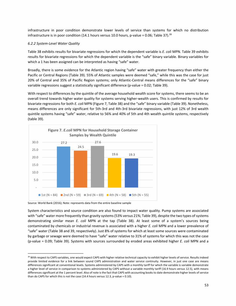
53

infrastructure in poor condition demonstrate lower levels of service than systems for which no distribution

infrastructure is in poor condition (14.1 hours versus 10.0 hours, p‐value = 0.06; Table 37).39

6.2.2 System‐Level Water Quality

Table 38 exhibits results for bivariate regressions for which the dependent variable is E. coli MPN. Table 39 exhibits

results for bivariate regressions for which the dependent variable is the “safe” binary variable. Binary variables for

which a 1 has been assigned can be interpreted as having “safe” water.

Broadly, there is some evidence for the Atlantic region having “safe” water with greater frequency than either the

Pacific or Central Regions (Table 39). 55% of Atlantic samples were deemed “safe,” while this was the case for just

20% of Central and 35% of Pacific Region systems; only Atlantic‐Central means differences for the “safe” binary

variable regressions suggest a statistically significant difference (p‐value = 0.02; Table 39).

With respect to differences by the quintile of the average household wealth score for systems, there seems to be an

overall trend towards higher water quality for systems serving higher‐wealth users. This is confirmed by results for

bivariate regressions for both E. coli MPN (Figure 7, Table 38) and the “safe” binary variable (Table 39). Nonetheless,

means differences are only significant for 5th‐3rd and 4th‐3rd bivariate regressions, with just 12% of 3rd wealth

quintile systems having “safe” water, relative to 56% and 40% of 5th and 4th wealth quintile systems, respectively

(table 39).


System characteristics and source condition are also found to impact water quality. Pump systems are associated

with “safe” water more frequently than gravity systems (53% versus 21%; Table 39), despite the two types of systems

demonstrating similar mean E. coli MPN at the tap (Table 38). At least some of a system’s sources being

contaminated by chemicals or industrial revenue is associated with a higher E. coli MPN and a lower prevalence of

“safe” water (Table 38 and 39, respectively). Just 8% of systems for which at least some sources were contaminated

by garbage or sewage were deemed to have “safe” water relative to 31% of systems for which this was not the case

(p‐value = 0.09; Table 39). Systems with sources surrounded by eroded areas exhibited higher E. coli MPN and a

39 With respect to CAPS variables, one would expect CAPS with higher relative technical capacity to exhibit higher levels of service. Results indeed provide limited evidence for a link between sound CAPS administration and water service continuity. However, in just one case are means differences significant at conventional levels. Systems administered by CAPS with a monthly tariff for which the variable is variable demonstrate a higher level of service in comparison to systems administered by CAPS without a variable monthly tariff (16.9 hours versus 12.5), with means differences significant at the 1 percent level. Also of note is the fact that CAPS with accounting books to date demonstrate higher levels of service than do CAPS for which this is not the case (14.4 hours versus 12.3, p‐value = 0.10).

27.2 24.5

27.6

19.6 19.3

‐

5.0

10.0

15.0

20.0

25.0

30.0

Figure 7. E.coli MPN for Household Storage Container Samples by Wealth Quintile

1st (N = 84) 2nd (N = 59) 3rd (N = 69) 4th (N = 58) 5th (N = 55)

54

lower prevalence of “safe” water.40 Other system variables support the premise that systems with sources and

infrastructure in poor condition are associated with “safe” water with less frequency than systems with sources and

infrastructure for which this is not the case (Figure 8).

Bivariate regressions for which CAPS characteristics are the independent variables demonstrate few consistent

trends or significant relationships between the institutional strength of CAPS and water quality.


6.2.3 Household Water Quality

Results for household water quality regressions using storage container samples are shown for E. coli MPN in Table

40 and for the “safe” water binary variable in Table 41. P‐values in both cases were adjusted for clustering at the

community level.

The Atlantic again has the highest prevalence of “safe” water (41%; Table 41), despite also having the highest average

E. coli MPN compared to the Central and Pacific regions (Table 40). In no cases were means differences significant.

There is some evidence for improved water quality in the higher wealth quintiles (Table 40 and 41). Households

with an improved water source exhibit a higher percentage of “safe” water samples and lower average E. coli MPN

than those without an improved water source; in neither of these cases are means differences significant (Table 40

and 41). Households headed by individuals with higher levels of education (some secondary school or greater) have

“safer” water and lower E. coli MPN than households where household heads have lower levels of education.

Whereas 42% of households with “educated” household heads have “safe” water, this is the case for just 24% of

households with less educated household heads (p‐value = 0.05; Table 41). Gender may also be a factor in household

water quality, with households for which the female is the household member in charge of water exhibiting “safe”

water in storage containers less frequently than for male‐headed households (25% versus 40%, p‐value = 0.09).

However, households for which an “educated” woman oversees water exhibit “safe” water 40% of the time relative

to 25% for households in which this is not the case (p‐value = 0.11). This interaction variable is negative and

40 Means differences are significant (p‐value = 0.05) in the case of E. coli MPN but not in the case of the “safe” water binary variable (p‐value = 0.50).

32% 31%34%

27% 29%

24%

29%33%

29%

9% 8%5%

29%

21%

35%

25%

9%14%

0%

10%

20%

30%

40%

Figure 8. % of "safe" tap samples according to infrastructure condition

Does not have variable Has variable

55

TABLE 37: BIVARIATE REGRESSIONS FOR HOURS OF WATER SERVICE IN THE DRY SEASON BY SYSTEM AND CAPS VARIABLES OF INTEREST

Variable of interest Does not have variable

Has variable

Ttest

Obs. Mean (sd) Obs. Mean (sd) p‐value

Regional differences

Central = 0, Pacific = 1 128 14.08 (8.4) 66 10.87 (8.79) 0.01 ***

Atlantic = 0, Pacific = 1 25 17.82 (6.68) 66 10.87 (8.79) 0 ***

Atlantic = 0, Central = 1 25 17.82 (6.68) 128 14.08 (8.4) 0.04 **

Wealth quintile differences

5th = 0, 1st = 1 31 10.82 (8.69) 6 15.58 (7.73) 0.22

4th = 0, 1st = 1 65 13.86 (9.52) 6 15.58 (7.73) 0.67

3rd = 0, 1st = 1 64 13.42 (8.26) 6 15.58 (7.73) 0.54

2nd = 0, 1st = 1 53 14.64 (7.64) 6 15.58 (7.73) 0.77

5th = 0, 2nd = 1 31 10.82 (8.69) 53 14.64 (7.64) 0.04 **

4th = 0, 2nd = 1 65 13.86 (9.52) 53 14.64 (7.64) 0.63

3rd = 0, 2nd = 1 64 13.42 (8.26) 53 14.64 (7.64) 0.41

5th = 0, 3rd = 1 31 10.82 (8.69) 64 13.42 (8.26) 0.16

4th = 0, 3rd = 1 65 13.86 (9.52) 64 13.42 (8.26) 0.78

5th = 0, 4th = 1 31 10.82 (8.69) 65 13.86 (9.52) 0.14

System variables of interest

Pumped system = 0, Gravity system = 1 63 12.19 (9.28) 131 14.64 (7.9) 0.06

Any source in poor condition 164 14.08 (8.53) 33 12.28 (7.99) 0.26

Any source contaminated by garbage/sewage 171 13.71 (8.68) 38 13.03 (8.11) 0.66

Any source contaminated by chemicals/industrial residue 160 14.04 (8.74) 47 12.2 (7.94) 0.2

Any source not surrounded by green areas 185 13.72 (8.43) 24 12.59 (9.65) 0.54

Any source surrounded by eroded areas 159 13.71 (8.61) 49 13.17 (8.59) 0.7

Any source not protected 139 14.23 (8.78) 65 12.3 (7.95) 0.13

Treatment infra exists 141 13.16 (8.69) 71 14.57 (8.33) 0.26

Any treatment infra in poor condition 59 14.4 (8.33) 12 15.39 (8.62) 0.71

Storage infra exists 18 16.44 (8.22) 192 13.32 (8.59) 0.14

Any storage infra in poor condition 162 13.22 (8.72) 29 13.78 (8.1) 0.75

Distribution infra exists 6 10.82 (10.54) 205 13.66 (8.52) 0.42

Any distribution infra in poor condition 184 14.1 (8.55) 17 10.04 (7.82) 0.06

CAPS variables of interest

CAPS legalized 124 13.25 (8.3) 81 14.09 (8.84) 0.49

Technical staff paid 99 13.83 (8.49) 101 13.36 (8.56) 0.69

Has complaint‐receiving mechanism 91 13.62 (8.38) 110 13.6 (8.62) 0.99

Accountable to system‐users 77 12.4 (8.44) 120 14.23 (8.38) 0.14

Has monthly tariff 28 15.61 (7.7) 174 13.29 (8.59) 0.18

Monthly tariff is variable 151 12.51 (8.14) 51 16.88 (8.77) 0 ***

Accounting books to date 69 12.32 (8.83) 131 14.4 (8.22) 0.1

Provides preventative care 80 12.59 (8.6) 123 14.23 (8.42) 0.18

Protects area around source 15 13.44 (9.02) 187 13.72 (8.49) 0.9

Water treated with chlorine 135 13.35 (8.75) 76 13.99 (8.26) 0.6

Chlorine applied in last 15 days 186 13.62 (8.62) 26 13.74 (8.42) 0.94

*** Statistically significant at the 1 percent level, ** Statistically significant at the 5 percent level

56

TABLE 38: BIVARIATE REGRESSIONS FOR TAP SAMPLE E. coli MPN BY SYSTEM AND CAPS VARIABLES OF INTEREST ‐ SYSTEM LEVEL


Has variable

Ttest



Central = 0, Pacific = 1 54 22.56 (34.32) 17 31.8 (42.43) 0.36

Atlantic = 0, Pacific = 1 11 15.44 (31.61) 17 31.8 (42.43) 0.28

Atlantic = 0, Central = 1 11 15.44 (31.61) 54 22.56 (34.32) 0.53


5th = 0, 2nd = 1 9 12.45 (32.95) 22 23.62 (35.23) 0.42

4th = 0, 2nd = 1 20 27.93 (39.07) 22 23.62 (35.23) 0.71

3rd = 0, 2nd = 1 25 22.98 (34.63) 22 23.62 (35.23) 0.95

5th = 0, 3rd = 1 9 12.45 (32.95) 25 22.98 (34.63) 0.43

4th = 0, 3rd = 1 20 27.93 (39.07) 25 22.98 (34.63) 0.65

5th = 0, 4th = 1 9 12.45 (32.95) 20 27.93 (39.07) 0.31


Pumped system = 0, Gravity system = 1 19 23.33 (41.67) 58 23.76 (34.86) 0.97

Any source in poor condition 66 23.2 (34.93) 11 24.46 (40.36) 0.91

Any source contaminated by garbage/sewage 68 21.94 (34.5) 13 33.59 (42.15) 0.29

Any source contaminated by chemicals/industrial residue 62 19.35 (33.89) 19 38.37 (38.92) 0.04 **

Any source not surrounded by green areas 74 24 (35.74) 7 21.83 (39.32) 0.88

Any source surrounded by eroded areas 62 19.55 (32.61) 19 37.72 (42.75) 0.05 **

Any source not protected 55 23.67 (35.42) 26 24.12 (37.32) 0.96

Treatment infra exists 54 18.16 (32.75) 28 33.87 (39.31) 0.06

Any treatment infra in poor condition 24 37.59 (40.7) 4 11.54 (20.81) 0.23

Storage infra exists 7 12.61 (21.48) 73 24.07 (36.39) 0.42

Any storage infra in poor condition 61 25.86 (38.77) 11 16.24 (19.44) 0.43

Distribution infra exists 1 1.95 (.) 80 24.09 (35.95) 0.54

Any distribution infra in poor condition 72 24.96 (36.24) 7 18.17 (36.76) 0.64


CAPS legalized 42 29.29 (39.86) 35 18.38 (31.01) 0.19

Technical staff paid 34 22.17 (31.56) 43 26.04 (39.93) 0.65

Has complaint‐receiving mechanism 34 17.21 (33.26) 43 29.97 (37.96) 0.13

Accountable to system‐users 23 24.54 (38.76) 52 24.69 (36.12) 0.99

Has monthly tariff 8 21.59 (33.34) 69 24.65 (36.84) 0.82

Monthly tariff is variable 56 23.86 (35.31) 21 25.58 (39.69) 0.85

Accounting books to date 21 17.39 (35.37) 55 26.99 (36.94) 0.31

Provides preventative care 29 25.3 (39.23) 48 23.75 (34.82) 0.86

Protects area around source 6 42.74 (48.74) 71 22.78 (35.06) 0.2

Water treated with chlorine 51 26.8 (36.01) 30 18.74 (35.49) 0.33

Chlorine applied in last 15 days 70 23.56 (35.78) 12 23.33 (36.65) 0.98

Receive assistance with chlorine treatment 20 15.43 (26.5) 14 25.94 (43.01) 0.38


57

TABLE 39: BIVARIATE REGRESSIONS FOR BINARY VARIABLE MEASURING WHETHER WATER IS SAFE BY SYSTEM AND CAPS VARIABLES OF INTEREST ‐ SYSTEM LEVEL


Has variable

Ttest



Central = 0, Pacific = 1 54 20% (41%) 17 35% (49%) 0.21

Atlantic = 0, Pacific = 1 11 55% (52%) 17 35% (49%) 0.33

Atlantic = 0, Central = 1 11 55% (52%) 54 20% (41%) 0.02 **


5th = 0, 2nd = 1 9 56% (53%) 22 27% (46%) 0.14

4th = 0, 2nd = 1 20 40% (50%) 22 27% (46%) 0.39

3rd = 0, 2nd = 1 25 12% (33%) 22 27% (46%) 0.19

5th = 0, 3rd = 1 9 56% (53%) 25 12% (33%) 0.01 ***

4th = 0, 3rd = 1 20 40% (50%) 25 12% (33%) 0.03 **

5th = 0, 4th = 1 9 56% (53%) 20 40% (50%) 0.45


Pumped system = 0, Gravity system = 1 19 53% (51%) 58 21% (41%) 0.01 ***

Any source in poor condition 66 32% (47%) 11 9% (30%) 0.13

Any source contaminated by garbage/sewage 68 31% (47%) 13 8% (28%) 0.09

Any source contaminated by chemicals/industrial residue 62 34% (48%) 19 5% (23%) 0.01 ***

Any source not surrounded by green areas 74 27% (45%) 7 29% (49%) 0.93

Any source surrounded by eroded areas 62 29% (46%) 19 21% (42%) 0.5

Any source not protected 55 24% (43%) 26 35% (49%) 0.31

Treatment infra exists 54 28% (45%) 28 29% (46%) 0.94

Any treatment infra in poor condition 24 29% (46%) 4 25% (50%) 0.87

Storage infra exists 7 14% (38%) 73 29% (46%) 0.42

Any storage infra in poor condition 61 33% (47%) 11 9% (30%) 0.11

Distribution infra exists 1 0% (.%) 80 28% (45%) 0.54

Any distribution infra in poor condition 72 29% (46%) 7 14% (38%) 0.41


CAPS legalized 42 29% (46%) 35 26% (44%) 0.78

Technical staff paid 34 24% (43%) 43 30% (46%) 0.52

Has complaint‐receiving mechanism 34 35% (49%) 43 21% (41%) 0.16

Accountable to system‐users 23 26% (45%) 52 29% (46%) 0.81

Has monthly tariff 8 13% (35%) 69 29% (46%) 0.33

Monthly tariff is variable 56 23% (43%) 21 38% (50%) 0.2

Accounting books to date 21 24% (44%) 55 29% (46%) 0.65

Provides preventative care 29 17% (38%) 48 33% (48%) 0.13

Protects area around source 6 33% (52%) 71 27% (45%) 0.73

Water treated with chlorine 51 24% (43%) 30 33% (48%) 0.34

Chlorine applied in last 15 days 70 26% (44%) 12 42% (51%) 0.26

Receive assistance with chlorine treatment 20 35% (49%) 14 36% (50%) 0.97


58

TABLE 40: BIVARIATE REGRESSIONS FOR STORAGE SAMPLE E. coli MPN BY HOUSEHOLD VARIABLES OF INTEREST


Has variable

Ttest

Obs. Mean (sd) Obs. Mean (sd) p‐value1


Central = 0, Pacific = 1 198 22.01 (28.92) 90 24.61 (28.87) 0.66

Atlantic = 0, Pacific = 1 37 33.94 (37.24) 90 24.61 (28.87) 0.39

Atlantic = 0, Central = 1 37 33.94 (37.24) 198 22.01 (28.92) 0.24


5th = 0, 1st = 1 55 19.31 (25.36) 84 27.21 (33.72) 0.18

4th = 0, 1st = 1 58 19.58 (25.15) 84 27.21 (33.72) 0.17

3rd = 0, 1st = 1 69 27.58 (30.76) 84 27.21 (33.72) 0.95

2nd = 0, 1st = 1 59 24.46 (32.08) 84 27.21 (33.72) 0.61

5th = 0, 2nd = 1 55 19.31 (25.36) 59 24.46 (32.08) 0.4

4th = 0, 2nd = 1 58 19.58 (25.15) 59 24.46 (32.08) 0.38

3rd = 0, 2nd = 1 69 27.58 (30.76) 59 24.46 (32.08) 0.6

5th = 0, 3rd = 1 55 19.31 (25.36) 69 27.58 (30.76) 0.12

4th = 0, 3rd = 1 58 19.58 (25.15) 69 27.58 (30.76) 0.11

5th = 0, 4th = 1 55 19.31 (25.36) 58 19.58 (25.15) 0.96

Household variables of interest

Improved Water Source 65 26.57 (31.44) 260 23.47 (29.77) 0.52

Connected to Community System 136 27.04 (32.01) 189 21.97 (28.52) 0.24

Some Secondary School or more 282 25.28 (30.83) 43 16.31 (23.5) 0.04 **

Female Member Manages Household Water 38 20.86 (28.52) 284 24.41 (30.07) 0.45

Female with Secondary or more Manages Water 287 24.73 (30.39) 35 17.93 (24.72) 0.16

Last drink treated through chlorination 252 22.92 (30.79) 70 27.85 (26.14) 0.29

Firm Floor = 0, Earth Floor = 1 124 22.4 (26.64) 188 25.03 (32.04) 0.52

Zinc Roof = 1, Other Type of Roof = 0 42 24.62 (29.58) 281 23.74 (29.97) 0.86

Open defecation 292 24.93 (30.26) 33 16.63 (27.81) 0.12

Feces in Yard 213 22.29 (27.19) 112 27.52 (34.81) 0.24

Reports Handwashing Station 88 22.43 (31.36) 237 24.71 (29.65) 0.59

Station Convenient Location 98 23.3 (31.25) 227 24.43 (29.64) 0.78

Water and soap avail at handwashing station 109 24.54 (32.17) 216 23.86 (29.06) 0.87

Wide‐mouthed storage container 38 22.77 (29.02) 238 25.71 (30.57) 0.56 1 p‐values adjusted for clustering at community level; *** Statistically significant at the 1 percent level, ** Statistically significant at the 5 percent level

59

TABLE 41: BIVARIATE REGRESSIONS FOR BINARY VARIABLE MEASURING WHETHER WATER IS SAFE BY HOUSEHOLD VARIABLES OF INTEREST


Has variable

Ttest

Obs. Mean (sd) Obs. Mean (sd) p‐value1


Central = 0, Pacific = 1 198 26% (44%) 90 22% (42%) 0.63

Atlantic = 0, Pacific = 1 37 41% (50%) 90 22% (42%) 0.24

Atlantic = 0, Central = 1 37 41% (50%) 198 26% (44%) 0.33


5th = 0, 1st = 1 55 35% (48%) 84 25% (44%) 0.34

4th = 0, 1st = 1 58 29% (46%) 84 25% (44%) 0.54

3rd = 0, 1st = 1 69 28% (45%) 84 25% (44%) 0.74

2nd = 0, 1st = 1 59 19% (39%) 84 25% (44%) 0.32

5th = 0, 2nd = 1 55 35% (48%) 59 19% (39%) 0.12

4th = 0, 2nd = 1 58 29% (46%) 59 19% (39%) 0.16

3rd = 0, 2nd = 1 69 28% (45%) 59 19% (39%) 0.25

5th = 0, 3rd = 1 55 35% (48%) 69 28% (45%) 0.5

4th = 0, 3rd = 1 58 29% (46%) 69 28% (45%) 0.82

5th = 0, 4th = 1 55 35% (48%) 58 29% (46%) 0.57

Household variables of interest

Improved Water Source 65 23% (42%) 260 28% (45%) 0.52

Connected to Community System 136 27% (45%) 189 26% (44%) 0.91

Some Secondary School or more 282 24% (43%) 43 42% (50%) 0.05 **

Female Member Manages Household Water 38 39% (50%) 284 25% (44%) 0.09

Female with Secondary or more Manages Water 287 25% (44%) 35 40% (50%) 0.11

Last drink treated through chlorination 252 30% (46%) 70 17% (38%) 0.03 **

Firm Floor = 0, Earth Floor = 1 124 27% (45%) 188 26% (44%) 0.83

Zinc Roof = 1, Other Type of Roof = 0 42 21% (42%) 281 28% (45%) 0.4

Open defecation 292 26% (44%) 33 33% (48%) 0.47

Feces in Yard 213 24% (43%) 112 31% (47%) 0.27

Reports Handwashing Station 88 35% (48%) 237 24% (43%) 0.08

Station Convenient Location 98 34% (48%) 227 24% (43%) 0.13

Water and soap avail at handwashing station 109 32% (47%) 216 24% (43%) 0.21

Wide‐mouthed storage container 38 24% (43%) 238 25% (44%) 0.85


60

significant in a simple regression including gender and education independent variables, indicating that this

subgroup may in fact be associated with improved water quality.41

7. Discussion

The above analyses of the PROSASR IE sample lead us to several observations about the IE, itself, in addition to the

general WSS situation in rural Nicaragua at the time baseline data were collected. First, the IE sample we describe

in this paper appears to be fairly representative of poor rural households in Nicaragua. However, it differs from the

2011 DHS rural sample in ways possibly related to the target population and eligibility constraints of the IE. For

example, households in our sample appear to have a higher prevalence of concrete/tile floors relative to earth/dirt

floors, increased access to a sanitation facility, and increased connectivity to a community water system. This may

also be indicative of general improvements in household economy and of efforts on the part of the Nicaraguan

government to expand access to WSS services (e.g., temporal changes in living standards since 2011). It may also be

because PROSASR targets water systems likely to show improvements through PROSASR’s capacity‐building efforts.

This targeting could be correlated with “better off” communities; to the extent that less well‐off households (e.g.,

households with an increased prevalence of earth/dirt floors versus concrete/tile) without access to a sanitation

facility and/or community water system connection have systems that would be less likely to benefit from PROSASR,

these households may have been left out of the IE sample frame. Our sample frame also relied on the availability of

SIASAR data; systematic differences between methodologies for SIARSAR and DHS data collection and reliability

could explain some of the differences between the samples.

Second, results from balance checks indicate that treatment and control households are well‐balanced with respect

to measurable characteristics. Assessments of baseline balance do suggest specific indicators that are not balanced

and could be of importance to follow‐up outcomes. For example, balance checks suggest that control households

may be more likely to have taken their last drink from the tap, while treatment households are more likely to have

taken their last drink from a storage container. Additionally, average E. coli MPN for tap samples for households

taking their last glass from the tap was higher among treatment households than control households. Nonetheless,

it appears that randomization was largely successful at ensuring a balance across the majority of observed baseline

characteristics. At follow‐up, variables for which means differences between the treatment and control group were

significant will be controlled for to assess whether imbalances in these variables impact our interpretation of results.

Baseline data suggest that access to a water system is not uniform across regions and wealth quintiles in our sample.

The Pacific region exhibits the highest prevalence of connectivity (66%) relative to the Atlantic and Central regions

(62% and 59%, respectively) (Table 8). Pacific households are also wealthier, on average, than households in the

Atlantic and Central regions (Figure 3). Across all regions, wealthier households exhibited higher levels of access to

a community system, as well as access to an improved water source and improved sanitation (Table 9).

Results from our assessment of correlates of water system sustainability and quality suggest that the Atlantic region

has some advantages over the Central and Pacific regions. Households in the Atlantic region report 17.6 hours of

service a day during the dry season, on average, relative to 11.6 and 13.7 hours of service a day in the Central and

Pacific regions, respectively (Table 8). Bivariate regressions for household service levels aggregated at the system

level (Figure 5; Table 37) confirm that the rain‐heavy Atlantic exhibits increased service levels relative to the Pacific

and Central regions. Samples taken from the taps of water systems in the Atlantic were safe in 55% of systems

relative to 35% and 20% of systems in the Pacific and Central regions, respectively (Table 39).

Our analysis also provides some evidence that systems serving wealthier households exhibit higher quality water

than do systems serving less‐wealthy households, but, perhaps counterintuitively, fewer hours of service. In terms

41 With regards to other household variables of interest, we find that, counterintuitively, households claiming that they had treated their last drink of water through chlorination exhibit lower levels of “safe” water than households not treating their last drink through chlorination (p‐value = 0.03). At the same time, given that an analysis of the chlorine samples taken at the household level indicated that very few households chlorinated water, there is little reason to read much into this result.

61

of water quality, results from bivariate regressions indicate that 56% of systems serving households at the top wealth

quintile exhibit safe water relative to 40% and 12% of systems serving households in the fourth and third wealth

quintiles, respectively (Table 39). However, households in the top wealth quintile report receiving just 12.2 hours of

service a day during the dry season in comparison to 14.8 hours a day for households in the bottom wealth quintile

(Table 14). Households in the top wealth quintile are also more likely to experience service interruptions than poorer

households (Table 14). Lower levels of service for wealthier households may be due to higher overall water

consumption on their part versus poorer households (Table 14), possibly contributing to increased pressure on water

systems. Alternatively, increased interruptions and reduced service time among wealthier households may also

reflect CAPS that are proactively managing water systems in response to dry season stresses and the actual capacity

of system sources.

Differences in water quality across wealth quintiles and regions may be related to the presence or absence of system

infrastructure components, as well as the condition of infrastructure components. For example, pump systems,

which are more prevalent among systems serving wealthier households (Table 19), exhibit safe water with greater

frequency than gravity systems, which are more prevalent among systems serving poorer households (53% and 21%,

respectively; Table 39). Additionally, systems with some sources in poor condition (less common among wealthier

households; Table 19) are less likely to have safe water than systems with no sources in poor condition (9% and 32%,

respectively; p‐value = 0.13; Table 39). Other variables correlated with decreased prevalence of safe water (i.e., any

source contaminated with garbage and/or sewage and any source contaminated with chemicals and/or industrial

residue) do not appear correlated with household wealth quintiles. There is also evidence that other variables

related to system infrastructure are correlated with water quality (i.e., condition of storage and treatment

infrastructure).

Bivariate regressions also illuminate correlations between system infrastructure and water system service levels. For

one, even though gravity systems are associated with lower prevalence of safe water relative to pump systems, they

are associated with higher levels of service (Table 37). This finding may be related to the fact that gravity systems

are more prevalent among systems serving poorer households, which also exhibit higher levels of water service,

while pump systems are more prevalent among systems serving wealthier households (Table 19). Secondly, even

though several variables demonstrate the general relationships we would expect to see between the prevalence of

certain infrastructure and service levels (i.e., any sources in poor condition and any sources contaminated by garbage

and/or sewage correlated with lower service levels), means differences are not significant for any of these variables

at conventional levels. Only means differences for any sources not being protected (p‐value = 0.13; Table 37), storage

infrastructure existing (p‐value = 0.14), and any distribution in poor condition (p‐value = 0.06), whereby a system

with said characteristic presents lower service levels, approach conventional levels of significance.

We found that relative administrative capacity levels among CAPS increased with the wealth level of households

served by the CAPS. For instance, just 35% of CAPS are legalized, even though more than 50% of CAPS serving

households at the top two wealth quintiles are legalized compared to 0% and 28% of CAPS serving the bottom two

wealth quintiles, respectively (Table 21). Trends for the prevalence of technical staff, paid technical staff, CAPS

having complaint‐receiving mechanisms, and CAPS being accountable to system users indicate that a higher

percentage of CAPS serving wealthier households have these administrative capacity characteristics than CAPS

serving poorer households. However, bivariate regressions provide little evidence that these and other CAPS

characteristics impact water quality and water service levels. There is, however, some evidence that variable tariffs

and accounting books being to date appear correlated with improved service levels (Table 37).42

42 Variable tariffs ensure that incentives are aligned such that tariff amounts are commensurate to water usage (e.g., if a household uses more water, it pays a higher tariff). Decreased water consumption may apply less pressure on water systems, potentially allowing them to provide water for a greater number of hours per day. Accounting books being to date may be reflective of increased administrative capacity on the part of CAPS.

62

In addition to insight into the correlates of water quality at the system level, our analysis also provides some insight

into WSS behavior at the household level. For one, households collect water from storage containers more

frequently than from the tap (84% and 14%, respectively; Table 12). Water samples from household storage

containers exhibited higher levels of E. coli MPN (Table 26) and were considered safe less frequently than water

coming from the tap (for samples from the household source from which the last drink was taken; Table 27). For

paired storage container‐tap samples, water from storage containers exhibited higher E. coli MPN (on average, 6.2

E. coli MPN; Table 26) compared to samples taken from the tap. Poorer relative water quality in storage containers

versus the tap would be less of an issue were households treating drinking water through chlorination. However,

despite 20% of households claiming to treat water through chlorination (Table 12), we found almost no evidence of

free or total chlorine in household water samples (data not shown). More than half of households said that they did

not treat water because someone told them that it was not necessary or their local CAPS told them that water had

already been treated (Table 12). Yet, there was little evidence that systems treated their water, or that chlorine was

present in the water when treatment was reported.

The bivariate regression results for water quality at the household level presented in Tables 40 and 41 do provide us

with some insight into the correlates of water quality at the household level. For one, there is some evidence for

water quality in storage containers being higher for households in higher wealth quintiles than poorer wealth

quintiles (i.e., means differences for 5th‐3rd and 4th‐3rd comparisons in Table 40, 5th‐2nd and 4th‐2nd comparisons

in Table 41). Secondly, there is evidence that households in which the household head has some secondary school

education or greater exhibit higher quality water in household storage containers. There is also evidence that

households for which a female household member manages the water supply exhibit safe water with less frequency

than households for which the household member is a male; however, the group of female household heads with

some secondary school education or more exhibit lower E. coli MPN levels and safe water with greater frequency

relative to households for which this is not the case. Household sanitation practices may also impact water quality

in storage containers: households practicing open defecation exhibit higher E. coli MPN levels than households not

practicing open defecation (p‐value = 0.12; Table 40). At the same time, there are several variables for which means

differences are significant that demonstrate relationships counter to what would be expected (i.e., households

treating their last drink of water with chlorination and households that report having a handwashing station exhibit

lower frequencies of safe water than for households for which that is not the case; Table 41); however, these results

could be explained by reverse causality, where treatment and hygiene increased in response to a household illness.

In the context of PROSASR, results from these exploratory analyses may provide insight to areas of future emphasis

for the capacity‐building of UMAS. For example, results indicate that capacity‐building may want to emphasize

support for maintaining distribution infrastructure in good condition and providing preventative care to systems to

ensure a high service levels. Additionally, the positive relationship between source condition (i.e., contamination,

not being surrounded by eroded areas) and service levels may imply that capacity‐building should emphasize the

need to protect and maintain system sources. Additionally, variable tariffs may act as a means incentivizing

sustainable use of water by households.

The primary purpose of baseline data collection is to establish the effectiveness of randomization at creating

comparable treatment groups. Baseline data collection activities can also provide key insights for follow‐up data

collection activities. In this context, baseline data collection relied heavily on existing SIASAR modules for system,

community, and CAPS surveys. SIASAR modules were designed for implementation across many countries and

contexts, and this broad approach led to some challenges with comprehension and execution among enumerators

and respondents in this specific (Nicaraguan) application. During follow‐up data collection, SIASAR modules will be

more carefully adapted to the specific context of this IE based on baseline experiences. Additionally, the IE team

plans on validating SIASAR indicator definitions with FISE in anticipation of follow‐up data collection activities. During

baseline, the conditions and speed of implementation also created some challenges with respect to data collection,

data management, and water sample collection. In the field and in the data, inconsistencies in E. coli results were

discovered that highlighted the need for improved training and quality control approaches for follow‐up. Specifically,

63

to ensure high quality water samples at IE follow‐up and in the context of other IEs, more emphasis should be put

on (i) adequate training of enumerators in the administration of water samples and (ii) monitoring the administration

of water sampling to ensure that any errors are corrected early on in data collection efforts. Accordingly, quality

assurance will be a focus during follow‐up data collection. We have no reason to believe that any measurement

errors introduced by these data collection challenges were differential with respect to treatment arm, further

indicating that the primary finding of balanced treatment arms is unbiased. Analysis of bivariate regressions and

lessons with respect to data collection and indicator definition should increase the likelihood of collecting high

quality data during PROSASR follow‐up data collection and IE efforts in the context of other rural water sustainability

projects.

8. Conclusion

This report presented descriptive statistics and analyses as they relate to a baseline survey conducted in 2016 in the

context of an IE which attempts to explain the causal impact of a large‐scale rural WSS program in Nicaragua. Data

were collected to assess current levels of functionality and durability of community water systems, the capacity of

service providers to administer systems sustainably, as well as the current state of WSS services at the community

and household level for treatment and control groups. Our results suggest that randomization of program treatment

resulted in balance across treatment and control groups. Additionally, several indicators were used to identify the

correlates of rural water system sustainability, including system characteristics (i.e., source condition, the presence

and condition of water system infrastructure components) and service provider characteristics (i.e., variable tariffs,

providing preventative care). Analyses were used to inform potential areas which PROSASR capacity‐building efforts

may want to emphasize to positively impact the sustainability of water systems. Lastly, we pointed out several areas

of improvement as they relate to data collection and indicator definitions that we hope will inform data collection

activities at follow‐up (2018), as well as other IEs in the context of rural water system sustainability.

64

ANNEX I: SUMMARY OF DATA COLLECTED FOR PROSASR IMPACT EVALUATION

Level of data collection Informant Sample size Data collected

Household Household head 4,850

Household head and members Household infrastructure Assets Water source Sanitation conditions Hand hygiene Environmental hygiene Waterborne illness prevalence Water quality

Community CAPS president, other official, or community leader

300

General characteristics (i.e., # households, schools, health post) Water and sanitation characteristics Infrastructure (i.e., electricity, internet)

System CAPS president or other official 316 Infrastructure (i.e., age, # users, technology) Source and infrastructure condition Water quality

Community Water Board (CAPS) CAPS president or other official 299

Institutional strength Financial sustainability Operations & Management Resources Government assistance

Municipal Technical Assistance Provider (UMAS)

UMAS manager or other official 77 Technical assistance to CAPS Budget Resources

65

ANNEX II: MEAN, STANDARD DEVIATION, AND PCA COMPONENT 1 WEIGHT FOR CREATION OF HOUSEHOLD WEALTH INDEX

Asset Mean Standard Deviation Weight

Radio 0.60 0.49 ‐0.03

Television 0.64 0.48 0.29

Refrigerator 0.25 0.43 0.33

Iron 0.34 0.47 0.31

Grinding Machine 0.35 0.48 ‐0.04

Cassette Recorder 0.06 0.24 0.10

Stereo Component 0.20 0.40 0.27

Fan 0.21 0.41 0.29

Blender 0.17 0.38 0.32

Sewing Machine 0.07 0.25 0.11

Bicycle 0.28 0.45 0.18

Motorcycle 0.14 0.35 0.18

Disc Player 0.19 0.39 0.27

Cell Phone 0.65 0.48 0.20

Computer 0.02 0.15 0.16

Connection Community System 0.62 0.48 0.11

Improved Sanitation 0.40 0.49 0.08

Open Defecation 0.11 0.31 ‐0.13

Wash Station 0.70 0.46 0.12

Burns Trash 0.81 0.39 ‐0.05

Firm Floor (concrete, tile) 0.42 0.49 0.29

Wood Floor 0.03 0.16 ‐0.01

Earthen Floor 0.56 0.50 ‐0.29

Zinc Sheet Roof 0.88 0.32 0.06

Tiled Roof 0.10 0.30 ‐0.06

Fiberglass/Asbestos Roof 0.01 0.09 0.01

Non‐permanent Roof (palm) 0.01 0.10 ‐0.05

66

References

Arnold, B., Arana, B., Mausezahi, D., Hubbard, A., Colford, J. (2009) Evaluation of pre‐existing three‐year household

water treatment and handwashing intervention in rural Guatemala. International Journal of Epidemiology. Vol 38

No. 6.

Barr Timothy and Tom Ash. (2015). Sustainable Water Rate Design at the Western Municipal Water District: The Art

of Revenue Recovery, Water use Efficiency and Customer Equity. In: Dinar, A., V. Pochat, and J. Albiac (Eds.), Water

Pricing Experiences and Innovations. Berlin: Springer.

Benova, L., Cumming, O. and Campbell, O. M. (2014). Systematic review and meta�analysis: association between water and sanitation environment and maternal mortality. Tropical Medicine & International Health, 19, 368‐387.

Bhandari, B. and Grant, M. (2007) User satisfaction and sustainability of drinking water schemes in rural communities

of Nepal . Sustainability : Science, Practice, & Policy 3.1

Briscoe, J. Furtado de Castro, P., Griffin, C., North, J. and Olsen, O. (1990) Toward Equitable and Sustainable Rural

Water Supplies: A Contingent Valuation Study in Brazil. World Bank Economic Review Vol. 4 (2): 115‐134

Carter, R. C., Tyrrel, S. F. and Howsam, P. (1999). The Impact and Sustainability of Community Water Supply and

Sanitation Programmes in Developing Countries. Water and Environment Journal, 13: 292–296.

Clasen, T. F., & Bastable, A. (2003). Faecal contamination of drinking water during collection and household storage:

the need to extend protection to the point of use. Journal of water and health, 1(3), 109‐115.

Dangour, A. D., Watson, L., Cumming, O., Boisson, S., Che, Y., Velleman, Y., Cavill, S., Allen, E. & Uauy, R. (2013).

Interventions to improve water quality and supply, sanitation and hygiene practices, and their effects on the

nutritional status of children. Cochrane Database Systematic Review, 8.

Del Borghi, A., Strazza, C., Gallo, M. et al. (2013) Water supply and sustainability: life cycle assessment of water

collection, treatment and distribution service. International Journal of Life Cycle Assessment Vol. 18 No. 1158.

DFID‐UKAid. (2012) Water, Sanitation and Hygiene Portfolio Review.

Dubios, A.E., Crump, J.A., Keswick, B.H., Slutsker, L., Quick, R.E., Vulule, J.M. and Luby, S.P. (2010) Determinants of

use of household‐level water chlorination products in rural Kenya. International Journal of Environmental Research

and Public Health. Vol. 7 I (10).

Dupont, D. (2014) “Water Conservation: Thinking Beyond the Tap,” in Dinar, A. and K. Schwabe (eds), Handbook of

Water Economics, Edward. Elgar Press. 32 ms pages.

ENDESA, 2011. <http://www.inide.gob.ni/endesa/Endesa11_12/BaseEndesa11.html> accessed October 2017.

EMNV, 2014. <http://www.inide.gob.ni/Emnv/Emnv14/EMNV%202014‐2%20Febrero%202016.pdf> accessed

October 2017.

Eneas da Silva et al. (2013) Developing sustainable and replicable water supply systems in rural communities in Brazil.

International Journal of Water Resources Development Volume 29, Issue 4

Etmannski and Darton (2013) Accounting for Sustainability in Bengal: Examining Arsenic‐Removal Technology using

Process Analysis Method Int. J. of Sustainable Water and Environmental SystemsVolume 4, No. 1

Fagan JE, Reuter MA, Langford KJ (2010) Dynamic performance metrics to assess sustainability and cost effectiveness

of integrated urban water systems. Resource Conservation Recovery 54:719–736

67

Ferraro, PJ, JJ Miranda Montero, M Price. (2011). Persistence of Treatment Effects with Norm‐based Policy

Instruments: evidence from a randomized environmental policy experiment. American Economic Review: papers and

proceedings. 101(3): 318–22.

Fewtrell, L., et al. (2005) Water, sanitation, and hygiene interventions to reduce diarrhea in less developed countries:

a systematic review and meta‐analysis. The Lancet infectious diseases. 5(1): p. 42‐52.

Foster, T. (2013) Predictors of sustainability for community‐managed handpumps in sub‐Saharan Africa: Evidence

from Liberia, Sierra Leone and Uganda. Environmental Science and Technology, 47(21): 12037‐12046

FONDO DE INVERSION SOCIAL DE EMERGENCIA (FISE), (2016). MANUAL DE ADMINISTRACIÓN DEL CICLO DE

PROYECTO MUNICIPAL‐MACPM, CAPÍTULO I: LA GESTION SOCIAL EN EL PROYECTO.

George, C. M., Oldja, L., Biswas, S., Perin, J., Lee, G. O., Kosek, M., Sack, R. B., Ahmed, S., Haque, R. & Parvin, T. (2015).

Geophagy is Associated with Environmental Enteropathy and Stunting in Children in Rural Bangladesh. The American

journal of tropical medicine and hygiene, 14‐0672.

Giné, R. and Pérez‐Foguet, A. (2008). Sustainability assessment of national rural water supply program in Tanzania.

Natural Resources Forum, 32: 327–342.

Gross, B., van Wijk, C. and Mukherjee, N. (2001) Linking Sustainability with Demand, Gender and Poverty: A study in

community‐managed water supply projects in 15 countries. IRC International Water and Sanitation Centre.

Harvey P.A., R.A. Reed. (2003) ”Sustainable rural water supply in Africa: Rhetoric and reality.”

Proceedings of the WEDC 29th Conference. Pages: 115�118. Hulland, K, Martin, N, Dreibelbis, R, DeBruicker, V and Winch, P (2015) What factors affect sustained adoption of

safe water, hygiene and sanitation technologies? 3ie Systematic Review Summary No. 2. Available at:

http://www.3ieimpact.org/media/filer_public/2015/08/23/srs_2‐_factors_for_sustained_wash_adoption.pdf

Hutton, G., Haller, L. and Bartram, J. (2007). Global cost‐benefit analysis of water supply and sanitation interventions.

Journal of water and health, 5, 481‐502.

Hutchings, P. Chan, Y.E. Cuadrado, L. Ezbakhe, F. Mesa, B. Tamekawa, C. Franceys, R. A systematic review of success

factors in the community management of rural water supplies over the past 30 years. Water Policy 17: 963–983.

INIDE (National Institute for Development Information), (2011). Encuesta Nicaragüense de Demografía y Salud

2011/12. Available at: http://ghdx.healthdata.org/record/nicaragua‐national‐demographic‐and‐health‐survey‐

2011‐2012

Jiménez, A. and Pérez‐Foguet, A. (2010b). Challenges for water governance in rural water supply: Lessons learned

from Tanzania. International Journal of Water Resources Development 26(2), 235–248.

Jiménez, A. and Pérez‐Foguet, A. (2011). The relationship between technology and functionality of rural water

points: Evidence from Tanzania. Water Science and Technology 63(5), 948–955.

Karamage, F., Zhang, C., Ndayisaba, F., Nahayo, L., Kayiranga, A., Omifolaji, J.K., Shao, H., Umuhoza, A., Nsengiyumva,

J.B. and Liu, T. (2016) The Need for Awareness of Drinking Water Loss Reduction for Sustainable Water Resource

Management in Rwanda. Journal of Geoscience and Environment Protection, Vol. 4, 74‐87

Kvarnström, E., McConville, J., Bracken, P., Johansso, M. and Fogde, M. (2011) The sanitation ladder – a need for a

revamp? Journal of Water, Sanitation and Hygiene for Development Vol 1 No 1 pp 3–12 IWA Publishing.

Levy, K., Nelson, K. L., Hubbard, A., & Eisenberg, J. N. (2008). Following the water: a controlled study of drinking

water storage in northern coastal Ecuador. Environmental health perspectives, 116(11), 1533.

68

Lockwood, H. 2002. Institutional support mechanisms for community‐managed rural water supply & sanitation

systems in Latin America. Strategic Report No. 6. Environmental Health Project (EHP). Washington, DC, US: USAID.

Lockwood, H. and Smits, S. 2011. Supporting rural water supply: Moving towards a service delivery approach. UK:

Practical Action Publishing.

Lockwood H.; Bakalian, A. and Wakeman, W. 2003. Assessing sustainability in rural water supply: The role of follow‐

up support to communities; Literature review and desk review of rural water supply and sanitation project

documents. Washington, DC: World Bank.

Lim, S. S., Vos, T., Flaxman, A. D., Danaei, G., Shibuya, K., Adair‐Rohani, H., Amann, M., Anderson, H. R., Andrews, K.

G. and Aryee, M. (2013). A comparative risk assessment of burden of disease and injury attributable to 67 risk factors

and risk factor clusters in 21 regions, 1990–2010: a systematic analysis for the Global Burden of Disease Study 2010.

The Lancet, 380, 2224‐2260.

Lundin, M., Molander, S., and Morrison, G. M. (1999). A set of indicators for the assessment of temporal variations

in sustainability of sanitary systems. Water Science and Technology, 39(5), 235–242.

Lyer, P., Davis, J., Yavuz, E. and Evans, B. (2002) Rural Water Supply, Sanitation and Hygiene: A Review of 25 Years of

World Bank Lending(1978–2003): Water Supply & Sanitation Working Notes, World Bank.

Mandara, C.G., Butjin, C., and Niehof, A. (2013) Community management and sustainability of rural water facilities

in Tanzania. Water Policy 15, 79‐100.

Mayer, Peter W., William B. DeOreo, et al. (1998). “Residential End Use Study Progress Report: Year 2.” AWWA

Annual Conference Proceedings, Dallas, TX.

Marks, S., Komices, K. and Davis, J. (2014) Community Participation and Water Supply Sustainability: Evidence from

Handpump Projects in Rural Ghana. Journal of Planning and Education Research. Sage Publication. 04‐041.

Mehta, L. and Movik, S. (2014) ‘Liquid dynamics: challenges for sustainability in the water domain’, WIREs Water 1:

369–84 <http://dx.doi.org/10.1002/wat2.1031>.

Mitchell, D. L. and Chesnutt, T.W. (2013). “Evaluation of East Bay Municipal Utility District’s Pilot of WaterSmart

Home Water Reports.” Report prepared for the California Water Foundation and East Bay Municipal Utility District.

Montgomery, M.A., Bartram, J. and Elimelech, M. (2009) Increasing Functional Sustainability of Water and Sanitation

Supplies in Rural Sub‐Saharan Africa. Environmental Engineering Science. 26(5): 1017‐1023.

doi:10.1089/ees.2008.0388.

Mukherjee, Nilanjana and van Wijk, Christina (2003) Sustainability planning and monitoring in community water

supply and sanitation. IRC International Water and Sanitation Centre.

Pullan, R. L., Freeman, M. C., Gething, P. W. and Brooker, S. J. (2014). Geographical Inequalities in Use of Improved

Drinking Water Supply and Sanitation across Sub‐Saharan Africa: Mapping and Spatial Analysis of Cross‐sectional

Survey Data. PLoS Med, 11, e1001626.

Ramesh, A., Blanchet, K., Ensink, J.H. and Roberts, B. (2015) Evidence on the Effectiveness of Water, Sanitation, and

Hygiene (WASH) Interventions on Health Outcomes in Humanitarian Crises: A Systematic Review. PLoS One. 10(9)

NCBI. Available at: https://www.ncbi.nlm.nih.gov/pubmed/26398228

Schouten, T. and Moriarty, P. 2003. Community water, community management; from system to service in rural

areas. London, UK: ITDG Publishing

69

Schmidt, W.P. and Cairncross, S. (2009). Household water treatment in poor populations: is there enough evidence

for scaling up now? Environmental science & technology, 43 (4), 986–992.

Schweitzer, R. and Mihelcic, J. (2012) Assessing sustainability of community management of rural water systems in

the developing world. Journal of Water, Sanitation and Hygiene for Development. Vol. 2 (1) 20‐30; DOI:

10.2166/washdev.2012.056

Snilstveit B. and Waddington H. (2009), "Effectiveness and sustainability of water, sanitation, and hygiene

interventions in combating diarrhoea", Journal of Development Effectiveness, Vol 1 Issue 3: 295–335.

Soley, Foster and Thøgersen, Jens (2003) Monitoring and evaluation system for rural water supply. Nigeria: 29th

WEDC International Conference blz 296‐298.

Sommer, M., Kjellen, M. and Pensulo, C. (2013). Girls' and women's unmet needs for menstrual hygiene

management (MHM): the interactions between MHM and sanitation systems in low‐income countries. Journal of

Water, Sanitation and Hygiene for Development, 3, 283‐297.

Spears, D. (2013). How much international variation in child height can sanitation explain? World Bank policy

research working paper.

Stanton BF and Clemens JD. (1987). An educational intervention for altering water‐sanitation behaviors to reduce

childhood diarrhea in urban Bangladesh. II. A randomized trial to assess the impact of the intervention on hygienic

behavior and rates of diarrhea. Am J Epidemiol. Feb. 1987, 125(2): 292─301.

Stocks ME, Ogden S, Haddad D, Addiss DG, McGuire C, Freeman MC (2014) Effect of Water, Sanitation, and Hygiene

on the Prevention of Trachoma: A Systematic Review and Meta‐Analysis. PLoS Med 11(2): e1001605.

doi:10.1371/journal.pmed.1001605.

Strunz, E.C., Addis, G.D., Stocks, M.E., Ogden, S., Utzinger, J., and Freeman, M.C. (2014) Water, sanitation, hygiene,

and soil‐transmitted helminth infection: a systematic review and meta‐analysis. PLoS Med.11(3) NCBI. Available at:

https://www.ncbi.nlm.nih.gov/pubmed/24667810

Taylor, D.L., Kahawita, T.M., Cairncross, S., Ensink, H. (2015). The Impact of Water, Sanitation and Hygiene

Interventions to Control Cholera: A Systematic Review. PLoS One. 10(8). Available at:

https://www.ncbi.nlm.nih.gov/pubmed/26284367

UNICEF (1999) Water Hand Book: Water, Environment and Sanitation Technical Guidelines Series ‐ No. 2

USAID (2009) Environmental guidelines for small‐scale activities in Africa: Chapter 16 water and sanitation.

Timmins, C. (2003). “Demand‐side Technology Standards Under Inefficient Pricing Regimes: Are They Effective Water

Conservation Tools in the Long Run?” Environmental and Resource Economics. 26: 107‐24.

Trevett, A. F., Carter, R. C., & Tyrrel, S. F. (2004). Water quality deterioration: a study of household drinking water

quality in rural Honduras. International journal of environmental health research, 14(4), 273‐283.

Whittington, D. et al. (2009) How well is the demand‐driven, community management model for rural water supply

systems doing? Evidence from Bolivia, Peru and Ghana. Water Policy. Vol 11 No 6. IWA Publishing.

Wutich, A. and Ragsdale, K. (2008). Water insecurity and emotional distress: coping with supply, access, and seasonal

variability of water in a Bolivian squatter settlement. Social science & medicine, 67, 2116‐2125.

Well (1998) DFID guidance manual on water supply and sanitation programs, WEDC, Loughborough University, UK,

1998

70

Whittington, D. Smith, V. K., Okorafor, A., Okore, A., Liu, JL. & Mcphail (1992) Giving Respondents Time to Think in

Contingent Valuation Studies: A Developing Country Application. Environmental Economic management 2:205‐545.

WHO/UNICEF (2014). Progress on Drinking Water and Sanitation ‐ 2014 Update. New York: WHO/UNICEF Joint

Monitoring Programme for Water and Sanitation. New York.

WHO/UNICEF. (2015). Progress on sanitation and drinking water: 2015 update and MDG assessment. World Health

Organization.

Wild, L. Chambers, V., King, M. and Harris, D. (2012) Common constraints and incentive problems in service delivery.

ODI Working Paper 351. U.K.

World Bank (2014). PROJECT APPRAISAL DOCUMENT ‐ SUSTAINABLE RURAL WATER SUPPLY AND SANITATION

SECTOR PROJECT.

World Bank (2015). NICARAGUA SUSTAINABLE RURAL WATER SUPPLY AND SANITATION PROJECT IMPACT

EVALUATION SIEF BASELINE VALIDATION REPORT.

Wright, J., Gundry, S. and Conroy, R. (2004). Household drinking water in developing countries: a systematic review

of microbiological contamination between source and point‐of‐use. Tropical Medicine & International Health, 9, 106‐

17.

WSP, 2011. Rural Water Supply and Sanitation Challenges in Latin America for the Next Decade. WSP‐WB

Washington D.C. <http://www.wsp.org/sites/wsp.org/files/publications/WSP‐LAC‐Rural‐Water‐Sanitation‐Next‐

Decade.pdf>

WSSCC, 2010. <http://www.wsscc.org/sites/default/files/publications/wsscc_hygiene_and_

sanitation_software_2010.pdf>

Documents

Increasing the Sustainability of Rural Water Service