Increased stray gas abundance in a subset of drinkingwater wells near Marcellus shale gas extractionRobert B. Jacksona,b,1, Avner Vengosha, Thomas H. Darraha, Nathaniel R. Warnera, Adrian Downa,b, Robert J. Poredac,Stephen G. Osbornd, Kaiguang Zhaoa,b, and Jonathan D. Karra,b

aDivision of Earth and Ocean Sciences, Nicholas School of the Environment and bCenter on Global Change, Duke University, Durham, NC 27708; cDepartmentof Earth and Environmental Sciences, University of Rochester, Rochester, NY 14627; and dGeological Sciences Department, California State PolytechnicUniversity, Pomona, CA 91768

Edited by Susan E. Trumbore, Max Planck Institute for Biogeochemistry, Jena, Germany, and approved June 3, 2013 (received for review December 17, 2012)

Horizontal drilling and hydraulic fracturing are transforming energyproduction, but their potential environmental effects remain contro-versial.We analyzed141drinkingwaterwells across theAppalachianPlateaus physiographic province of northeastern Pennsylvania, ex-amining natural gas concentrations and isotopic signatures withproximity to shale gas wells. Methane was detected in 82% ofdrinking water samples, with average concentrations six timeshigher for homes <1 km from natural gas wells (P = 0.0006). Eth-ane was 23 times higher in homes <1 km from gas wells (P =0.0013); propane was detected in 10 water wells, all within ap-proximately 1 km distance (P = 0.01). Of three factors previouslyproposed to influence gas concentrations in shallow groundwater(distances to gas wells, valley bottoms, and the Appalachian Struc-tural Front, a proxy for tectonic deformation), distance to gaswellswas highly significant for methane concentrations (P = 0.007; mul-tiple regression), whereas distances to valley bottoms and theAppalachian Structural Front were not significant (P = 0.27 andP = 0.11, respectively). Distance to gas wells was also the mostsignificant factor for Pearson and Spearman correlation analyses(P< 0.01). For ethane concentrations, distance to gas wells was theonly statistically significant factor (P < 0.005). Isotopic signatures(δ13C-CH4, δ13C-C2H6, and δ2H-CH4), hydrocarbon ratios (methaneto ethane and propane), and the ratio of the noble gas 4He to CH4

in groundwater were characteristic of a thermally postmatureMarcellus-like source in some cases. Overall, our data suggest thatsome homeowners living <1 km from gas wells have drinkingwater contaminated with stray gases.

carbon, hydrogen, and helium isotopes | groundwater contamination |geochemical fingerprinting | fracking | hydrology and ecology

Unconventional sources of gas and oil are transforming energysupplies in the United States (1, 2). Horizontal drilling and

hydraulic fracturing are driving this transformation, with shale gasand other unconventional sources now yielding more than one-half of all US natural gas supply. In January of 2013, for instance,the daily production of methane (CH4) in theUnited States rose to∼2 × 109 m3, up 30% from the beginning of 2005 (3).Along with the benefits of rising shale gas extraction, public

concerns about the environmental consequences of hydraulicfracturing and horizontal drilling are also growing (4, 5). Theseconcerns include changes in air quality (6), human health effectsfor workers and people living near well pads (5), induced seis-micity (7), and controversy over the greenhouse gas balance (8, 9).Perhaps the biggest health concern remains the potential fordrinking water contamination from fracturing fluids, naturalformation waters, and stray gases (4, 10–12).Despite public concerns over possible water contamination,

only a few studies have examined drinking water quality related toshale gas extraction (4, 11, 13).Working in theMarcellus region ofPennsylvania, we published peer-reviewed studies of the issue,finding no evidence for increased concentrations of salts, metals,or radioactivity in drinking water wells accompanying shale gasextraction (4, 11). We did find higher methane concentrations and

less negative δ13C-CH4 signatures, consistent with a natural gassource, in water for homeowners living<1 km from shale gas wells(4). Here, we present a more extensive dataset for natural gas inshallow water wells in northeastern Pennsylvania, comparing thedata with sources of thermogenic methane, biogenically derivedmethane, and methane found in natural seeps. We present com-prehensive analyses for distance to gas wells and ethane and pro-pane concentrations, two hydrocarbons that are not derived frombiogenic activity and are associated only with thermogenic sources.Finally, we use extensive isotopic data [e.g., δ13C-CH4, δ2H-CH4,δ13C-C2H6, δ13C-dissolved inorganic carbon (δ13C-DIC), andδ2H-H2O] and helium analysis (4He/CH4) to distinguish amongdifferent sources for the gases observed (14–16).Our study area (Figs. S1 and S2) is within the Appalachian

Plateaus physiographic province (17, 18) and includes six countiesin Pennsylvania (Bradford, Lackawanna, Sullivan, Susquehanna,Wayne, and Wyoming). We sampled 81 new drinking water wellsfrom the three principle aquifers (Alluvium, Catskill, and LockHaven) (Fig. S1) (11). We combined the data with results from 60previously sampled wells in Pennsylvania (4) and included a fewwells from the Genesee Formation in Otsego County of New York(4). The typical depth of drinking water wells in our study was 60–90 m (11). We also sampled a natural methane seep at Salt SpringsState Park in Franklin Forks, Pennsylvania (N 41.91397,W 75.8663;Susquehanna County) to compare with drinking water from homesin our study, some located within a few kilometers of the spring.Descriptions of the underlying geology, including the Marcellus

Formation found 1,500–2,500 m underground, are presented inrefs. 4 and 11 and Fig. S2. Previous researchers have characterizedthe region’s geology and aquifers (19–23). Briefly, the two majorbedrock aquifers are the Upper Devonian Catskill Formation,comprised primarily of a deltaic clastic wedge gray-green to gray-red sandstone, siltstone, and shale, and the underlying LockHaven Formation, consisting of interbedded fine-grained sand-stone, siltstone, and silty shale (19, 22, 24). The two formationscan be as deep as ∼1,000 m in the study area and have beenexploited elsewhere for oil and gas historically. The sedimentarysequences are gently folded and dip shallowly (1–3°) to the eastand south (Fig. S2), creating alternating exposures of synclinesand anticlines at the surface (17, 23, 25). These formations areoverlain by the Alluvium aquifer, comprised of unconsolidatedglacial till, alluvium sediments, and postglacial deposits foundprimarily in valley bottoms (20, 22).

Author contributions: R.B.J., A.V., T.H.D., N.R.W., and A.D. designed research; R.B.J., A.V.,T.H.D., N.R.W., A.D., R.J.P., S.G.O., K.Z., and J.D.K. performed research; R.B.J., A.V., T.H.D.,N.R.W., A.D., R.J.P., K.Z., and J.D.K. analyzed data; and R.B.J., A.V., T.H.D., N.R.W., andA.D. wrote the paper.

The authors declare no conflict of interest.

This article is a PNAS Direct Submission.

Freely available online through the PNAS open access option.1To whom correspondence should be addressed. E-mail: jackson@duke.edu.

This article contains supporting information online at www.pnas.org/lookup/suppl/doi:10.1073/pnas.1221635110/-/DCSupplemental.

www.pnas.org/cgi/doi/10.1073/pnas.1221635110 PNAS Early Edition | 1 of 6

ENVIRO

NMEN

TAL

SCIENCE

S

Results and DiscussionDissolved methane was detected in the drinking water of 82% ofthe houses sampled (115 of 141). Methane concentrations indrinking water wells of homes <1 km from natural gas wells (59of 141) were six times higher on average than concentrations forhomes farther away (P = 0.0006, Kruskal–Wallis test) (Fig. 1 andFig. S3). Of 12 houses where CH4 concentrations were greaterthan 28 mg/L (the threshold for immediate remediation set bythe US Department of the Interior), 11 houses were within 1-kmdistance of an active shale gas well (Fig. 1). The only exceptionwas a home with a value of 32 mg CH4/L at 1.4-km distance.Similar to the results for methane, concentrations of ethane

(C2H6) and propane (C3H8) were also higher in drinking waterof homes near natural gas wells (Fig. 1). Ethane was detected in40 of 133 homes (30%; 8 fewer homes were sampled for ethaneand propane than for methane). Propane was detected in waterwells in 10 of 133 homes, all approximately <1 km from a shalegas well (P = 0.01) (Fig. 1, Lower Inset). Ethane concentrationswere 23 times higher on average for homes <1 km from a gas well:0.18 compared with 0.008 mg C2H6/L (P = 0.001, Kruskal–Wallis).Seven of eight C2H6 concentrations >0.5 mg/L were found <1 km

from a gas well (Fig. 1), with the eighth point only 1.1 km away(Fig. 1). Moreover, the higher ethane concentrations all occurredin groundwater with methane concentrations>15 mg/L (P = 0.003for the regression of C2 and C1) (Fig. S4), although not all highermethane concentration waters had elevated ethane.Ratios of ethane to methane (C2/C1) and propane to methane

(C3/C1) were much higher for homes within ∼1 km of natural gaswells (Fig. 2). Our high C3/C1 samples were also an order ofmagnitude greater than in salt-rich waters from a natural methaneseep at the nearby Salt Springs State Park (mean [C3]/[C1] =0.000029 and [C3] = 0.0022 mg/L for the salt spring samples).Because microbes effectively do not produce ethane or propane inthe subsurface (26, 27), our observed values within ∼1 km ofdrilling seem to rule out a biogenic methane source, and they areconsistent with both wetter (higher C2 + C3 content) gases foundin the Marcellus Formation and our earlier observation of meth-ane in drinking water wells in the region (4).Along with distance to gas wells (4), proximity to both valley

bottom streams (i.e., discharge areas) (28) and the AppalachianStructural Front (ASF; an index for the trend in increasing thermalmaturity and degree of tectonic deformation) has been suggestedto influence dissolved gas concentrations. Of these factors, dis-tance to gas wells was the dominant statistical factor in our anal-yses for both methane (P = 0.0007) (Table 1, multiple regressionanalysis) and ethane (P < 0.005) (Table 1). In contrast, neitherdistance to the ASF (P = 0.11) nor distance to valley bottomstreams (P = 0.27) was significant for methane concentrationsanalysis using linear regression. For single correlation factors,distance to gas wells was again the dominant statistical term (P =0.0003 and P = 0.001 for Pearson and Spearman coefficients, re-spectively). Distance to the ASF was slightly significant by Pearsonand Spearman correlation analyses (P = 0.04 and P = 0.02, re-spectively), whereas distance to valley bottom streams was slightlysignificant only for the nonparametric Spearman analysis (P= 0.22for Pearson and P = 0.01 for Spearman) (Table 1). For observedethane concentrations, distance to gas wells was the only factor inour dataset that was statistically significant (P < 0.005, regardlessof whether analyzed by multiple regression, Pearson correlation,or Spearman analyses) (Table 1).

Fig. 1. Concentrations of (Upper) methane, (Lower) ethane, and (LowerInset) propane (milligrams liter−1) in drinking water wells vs. distance tonatural gas wells (kilometers). The locations of natural gas wells wereobtained from the Pennsylvania DEP and Pennsylvania Spatial Data Accessdatabases (54). The gray band in Upper is the range for considering hazardmitigation recommended by the US Department of the Interior (10–28 mgCH4/L); the department recommends immediate remediation for any value>28 mg CH4/L.

Fig. 2. The ratio of ethane to methane (C2/C1) and (Inset) propane tomethane (C3/C1) concentrations in drinking water wells as a function ofdistance to natural gas wells (kilometers). The data are plotted for all caseswhere [CH4], [C2H6], and [C3H8] were above detection limits or [CH4] was>0.5 mg/L but [C2H6] or [C3H8] was below detection limits using the de-tection limits of 0.0005 and 0.0001 mg/L for [C2H6] and [C3H8], respectively.

2 of 6 | www.pnas.org/cgi/doi/10.1073/pnas.1221635110 Jackson et al.

Isotopic signatures and gas ratios provide additional insight intothe sources of gases in groundwater. Signatures of δ13C-CH4 >−40‰ (reference to Vienna Pee Dee Belemnite standard) gen-erally suggest a thermogenic origin for methane, whereas δ13C-CH4 values < −60‰ suggest a biogenically derived methanesource (27, 29, 30). Across our dataset, the most thermogenicδ13C-CH4 signatures (i.e., most enriched in 13C) in drinking waterwere generally found in houses with elevated [CH4] <1 km fromnatural gas wells (Fig. 3A). In fact, all drinking water wells withmethane concentrations >10 mg/L, the US Department of Inte-rior’s threshold for considering remediation, have δ13C-CH4 sig-natures consistent with thermogenic natural gas. Our data alsoshow a population of homes near natural gas wells with water thathas δ13C-CH4 signatures that seem to be microbial in origin,specifically those homes shown in Fig. 3A, lower left corner. Thecombination of our δ13C-CH4 (Fig. 3A) and δ2H-CH4 data (Fig.3B) overall, however, suggests that a subset of homes near naturalgas wells has methane with a higher thermal maturity than homesfarther away.Analyses of δ13C-CH4 and δ13C-C2H6 can help constrain po-

tential sources of thermally mature natural gases (14, 15, 30).Because organic matter cracks to form oil and then natural gas,the gases initially are enriched in higher aliphatic hydrocarbonsC2 and C3 (e.g., C3 > C2 > C1; i.e., a relatively wet gas). Withincreasing thermal maturity, the heavier hydrocarbons are pro-gressively broken down, increasing the C1:C2

+ ratio and leadingto isotopic compositions that become increasingly heavier orenriched (31). In most natural gases, the isotopic composition(δ13C) of C3 > C2 > C1 (i.e., δ13C of ethane is heavier thanmethane). In thermally mature black shales, however, this ma-turity trend reverses, creating diagnostic isotopic reversals inwhich the δ13C-CH4 becomes heavier than δ13C-C2H6 (Δ13C =δ13C-CH4 − δ13C-C2H6 > 1) (14, 15, 28, 30, 32).For 11 drinking water samples in our dataset with sufficient

ethane to analyze isotopic signatures, 11 samples were located<1.1 km from drilling, and 6 samples exhibited clear isotopicreversals similar to Marcellus production gases (Fig. 4). Con-versely, five drinking water samples and spring water from SaltSprings State Park showed the more common trend consistentwith Upper Devonian production gases (Fig. 4). In the study area,these isotopic values suggest multiple sources for hydrocarbongases. The Upper Devonian gases are likely introduced into theshallow crust either by natural processes over geologic time orthrough leakage around the casing in the annular space of theproduction well. In contrast, natural gas with heavy δ13C-CH4 andΔ13C > 0 likely stems from Marcellus production gases or a mix-ture of Marcellus gases and other annulus gases that migrated tothe surface during drilling, well completion, or production.Similar to our data, independent CH4 measurements taken by

the US Environmental Protection Agency (EPA) in Dimock,Pennsylvania (Residential Data Reports found at http://www.epaosc.org/site/doc_list.aspx?site_id=7555) in January of 2012also show three δ13C-CH4 values in drinking water wells between

−24.98‰ and -29.36‰ δ13C-CH4 and five samples with δ13C-CH4 values in the range of Marcellus gas defined in ref. 28. Theheaviest methane isotopic signatures in the EPA samples

Table 1. Statistical analyses for [CH4] and [C2H6]

Distanceto gas wells

Distanceto streams

Distanceto ASF

[CH4]Multiple regression P = 0.0007 P = 0.27 P = 0.11Pearson r P = 0.0003 P = 0.22 P = 0.04Spearman ρ P = 0.007 P = 0.01 P = 0.02

[C2H6]Multiple regression P = 0.0034 P = 0.053 P = 0.45Pearson r P = 0.003 P = 0.36 P = 0.11Spearman ρ P = 0.004 P = 0.95 P = 0.21

Fig. 3. (A) Methane concentration, (B) δ2H-CH4, and (C) methane to ethane +propane ratio plotted against δ13C-CH4. The grayscale shading refers to (A)distance to nearest gas wells and (B and C) methane concentration. The solidlines in B distinguishing natural gas sources are from ref. 27; the mixed line inB comes from the standard mixing equations in ref. 14. C shows two hypo-thetical trajectories: simple mixing between thermogenically and biogeni-cally derived gas (lower curve) and either diffusive migration or a three-component mixture between Middle and Upper Devonian gases and shallowbiogenic gases (upper curve).

Jackson et al. PNAS Early Edition | 3 of 6

ENVIRO

NMEN

TAL

SCIENCE

S

(−24.98‰ δ13C-CH4) exceeded the values observed for ethane(−31.2‰ δ13C-C2H6), an isotopic reversal (Δ13C = 6.22‰)characteristic of Marcellus or other deeper gas compared withgases from Upper Devonian sequences (14, 28).Helium is an inert noble gas with a radiogenic isotope, 4He, that

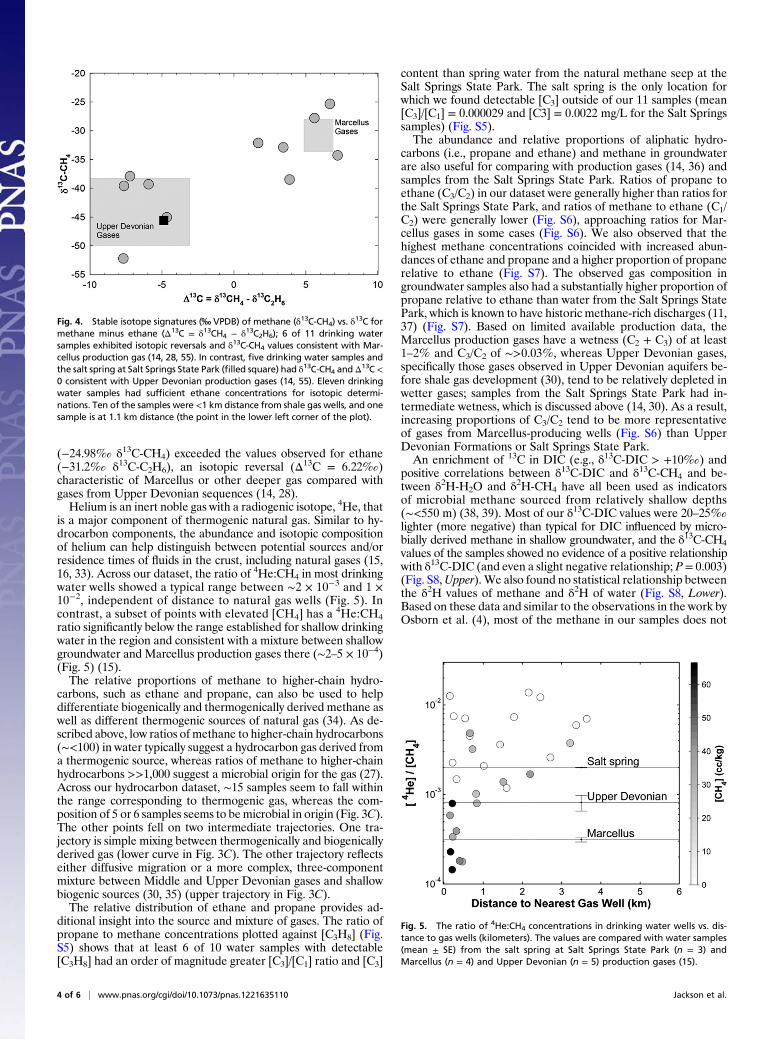
is a major component of thermogenic natural gas. Similar to hy-drocarbon components, the abundance and isotopic compositionof helium can help distinguish between potential sources and/orresidence times of fluids in the crust, including natural gases (15,16, 33). Across our dataset, the ratio of 4He:CH4 in most drinkingwater wells showed a typical range between ∼2 × 10−3 and 1 ×10−2, independent of distance to natural gas wells (Fig. 5). Incontrast, a subset of points with elevated [CH4] has a 4He:CH4ratio significantly below the range established for shallow drinkingwater in the region and consistent with a mixture between shallowgroundwater and Marcellus production gases there (∼2–5 × 10−4)(Fig. 5) (15).The relative proportions of methane to higher-chain hydro-

carbons, such as ethane and propane, can also be used to helpdifferentiate biogenically and thermogenically derived methane aswell as different thermogenic sources of natural gas (34). As de-scribed above, low ratios of methane to higher-chain hydrocarbons(∼<100) in water typically suggest a hydrocarbon gas derived froma thermogenic source, whereas ratios of methane to higher-chainhydrocarbons >>1,000 suggest a microbial origin for the gas (27).Across our hydrocarbon dataset, ∼15 samples seem to fall withinthe range corresponding to thermogenic gas, whereas the com-position of 5 or 6 samples seems to bemicrobial in origin (Fig. 3C).The other points fell on two intermediate trajectories. One tra-jectory is simple mixing between thermogenically and biogenicallyderived gas (lower curve in Fig. 3C). The other trajectory reflectseither diffusive migration or a more complex, three-componentmixture between Middle and Upper Devonian gases and shallowbiogenic sources (30, 35) (upper trajectory in Fig. 3C).The relative distribution of ethane and propane provides ad-

ditional insight into the source and mixture of gases. The ratio ofpropane to methane concentrations plotted against [C3H8] (Fig.S5) shows that at least 6 of 10 water samples with detectable[C3H8] had an order of magnitude greater [C3]/[C1] ratio and [C3]

content than spring water from the natural methane seep at theSalt Springs State Park. The salt spring is the only location forwhich we found detectable [C3] outside of our 11 samples (mean[C3]/[C1] = 0.000029 and [C3] = 0.0022 mg/L for the Salt Springssamples) (Fig. S5).The abundance and relative proportions of aliphatic hydro-

carbons (i.e., propane and ethane) and methane in groundwaterare also useful for comparing with production gases (14, 36) andsamples from the Salt Springs State Park. Ratios of propane toethane (C3/C2) in our dataset were generally higher than ratios forthe Salt Springs State Park, and ratios of methane to ethane (C1/C2) were generally lower (Fig. S6), approaching ratios for Mar-cellus gases in some cases (Fig. S6). We also observed that thehighest methane concentrations coincided with increased abun-dances of ethane and propane and a higher proportion of propanerelative to ethane (Fig. S7). The observed gas composition ingroundwater samples also had a substantially higher proportion ofpropane relative to ethane than water from the Salt Springs StatePark, which is known to have historic methane-rich discharges (11,37) (Fig. S7). Based on limited available production data, theMarcellus production gases have a wetness (C2 + C3) of at least1–2% and C3/C2 of ∼>0.03%, whereas Upper Devonian gases,specifically those gases observed in Upper Devonian aquifers be-fore shale gas development (30), tend to be relatively depleted inwetter gases; samples from the Salt Springs State Park had in-termediate wetness, which is discussed above (14, 30). As a result,increasing proportions of C3/C2 tend to be more representativeof gases from Marcellus-producing wells (Fig. S6) than UpperDevonian Formations or Salt Springs State Park.An enrichment of 13C in DIC (e.g., δ13C-DIC > +10‰) and

positive correlations between δ13C-DIC and δ13C-CH4 and be-tween δ2H-H2O and δ2H-CH4 have all been used as indicatorsof microbial methane sourced from relatively shallow depths(∼<550 m) (38, 39). Most of our δ13C-DIC values were 20–25‰lighter (more negative) than typical for DIC influenced by micro-bially derived methane in shallow groundwater, and the δ13C-CH4values of the samples showed no evidence of a positive relationshipwith δ13C-DIC (and even a slight negative relationship; P= 0.003)(Fig. S8,Upper).We also found no statistical relationship betweenthe δ2H values of methane and δ2H of water (Fig. S8, Lower).Based on these data and similar to the observations in the work byOsborn et al. (4), most of the methane in our samples does not

Fig. 4. Stable isotope signatures (‰ VPDB) of methane (δ13C-CH4) vs. δ13C formethane minus ethane (Δ13C = δ13CH4 − δ13C2H6); 6 of 11 drinking watersamples exhibited isotopic reversals and δ13C-CH4 values consistent with Mar-cellus production gas (14, 28, 55). In contrast, five drinking water samples andthe salt spring at Salt Springs State Park (filled square) had δ13C-CH4 and Δ13C <0 consistent with Upper Devonian production gases (14, 55). Eleven drinkingwater samples had sufficient ethane concentrations for isotopic determi-nations. Ten of the samples were <1 km distance from shale gas wells, and onesample is at 1.1 km distance (the point in the lower left corner of the plot).

Fig. 5. The ratio of 4He:CH4 concentrations in drinking water wells vs. dis-tance to gas wells (kilometers). The values are compared with water samples(mean ± SE) from the salt spring at Salt Springs State Park (n = 3) andMarcellus (n = 4) and Upper Devonian (n = 5) production gases (15).

4 of 6 | www.pnas.org/cgi/doi/10.1073/pnas.1221635110 Jackson et al.

seem to be derived locally in the shallow aquifers, and the gascomposition is not consistent with extensive microbial productionfrom methanogenesis or sulfate reduction. Methanotrophy alsodoes not seem to be occurring broadly across our dataset; it woulddecrease [CH4] and C1:C2 ratios and increase δ13CH4 values,reducing the differences that we observed for distance to gaswells. Overall, the combined results suggest that natural gas, de-rived at least in part from thermogenic sources consistent withMiddle Devonian origin, is present in some of the shallow waterwells <1 km away from natural gas wells.The two simplest explanations for the higher dissolved gas

concentrations that we observed in drinking water are (i) faulty orinadequate steel casings, which are designed to keep the gas andany water inside the well from leaking into the environment, and(ii) imperfections in the cement sealing of the annulus or gapsbetween casings and rock that keep fluids from moving up theoutside of the well (4, 40–42). In 2010, the Pennsylvania De-partment of Environmental Protection (DEP) issued 90 violationsfor faulty casing and cementing on 64 Marcellus shale gas wells;119 similar violations were issued in 2011.Distinguishing between the two mechanisms is important be-

cause of the different contamination to be expected through time.Casing leaks can arise from poor thread connections, corrosion,thermal stress cracking, and other causes (43). If the protectivecasing breaks or leaks, then stray gases could be the first sign ofcontamination, with less mobile salts and metals from formationwaters or chemicals from fracturing fluids potentially coming later.In contrast, faulty cement can allowmethane and other gases fromintermediate layers to flow into, up, and out of the annulus intoshallow drinking water layers. In such a scenario, the geochemicaland isotopic compositions of stray gas contamination would notnecessarily match the target shale gas, and no fracturing chemicalsor deep formation waters would be expected, because a directconnection to the deepest layers does not exist; also, such watersare unlikely to migrate upward. Comprehensive analyses of wellintegrity have shown that sustained casing pressure from annulargas flow is common. A comprehensive analysis of ∼15,500 oil andgas wells (43) showed that 12% of all wells drilled in the outercontinental shelf area of the Gulf of Mexico had sustained casingpressure within 1 y of drilling, and 50–60% of the wells had it from15 y onward. For our dataset, there is a weak trend to highermethane concentrations with increasing age of the gas wells (P =0.067 for [CH4] vs. time since initial drilling). This result couldmean that the number of drinking water problems may grow withtime or that drilling practices are improving with time; more re-search is needed before firm conclusions can be drawn.In addition to well integrity associated with casings or cement-

ing, two other potential mechanisms for contamination by hy-draulic fracturing/horizontal drilling include enhancing deep-to-shallow hydraulic connections and intersecting abandoned oil andgas wells. Horizontal drilling and hydraulic fracturing can stimu-late fractures or mineralized veins, increasing secondary hydraulicconnectivity. The upward transport of gases is theoretically pos-sible, including pressure-driven flow through open, dry fracturesand pressure-driven buoyancy of gas bubbles in aquifers and wa-ter-filled fractures (44, 45). Reduced pressures after the fracturingactivities could also lead to methane exsolving rapidly from solu-tion (46). If methane were to reach an open fracture pathway,however, the gas should redissolve into capillary-bound water and/or formation water, especially at the lithostatic and hydrostaticpressures present at Marcellus depths. Legacy or abandoned oiland gas wells (and even abandoned water wells) are another po-tential path for rapid fluid transport. In 2000, the PennsylvaniaDEP estimated that it had records for only 141,000 of 325,000 oiland gas wells drilled historically in the state, leaving the status andlocation of ∼184,000 abandoned wells unknown (47). However,historical drilling activity is minimal in our study area of north-eastern Pennsylvania, making this mechanism unlikely there.

This study examined natural gas composition of drinking waterusing concentration and isotope data for methane, ethane, pro-pane, and 4He. Based on the spatial distribution of the hydro-carbons (Figs. 1 and 2), isotopic signatures for the gases (Figs. 3and 4), wetness of the gases (Fig. 2 and Figs. S5, S6, and S7), andobserved differences in 4He:CH4 ratios (Fig. 5), we propose thata subset of homeowners has drinking water contaminated bydrilling operations, likely through poor well construction. Futureresearch and greater data disclosure could improve understandingof these issues in several ways. More research is needed across theMarcellus and other shale gas plays where the geological charac-teristics differ. For instance, a new study by Duke University andthe US Geological Survey showed no evidence of drinking watercontamination in a part of the Fayetteville Shale with a less frac-tured or tectonically deformed geology than the Marcellus andgood confining layers above and below the drinking water layers(48). More extensive predrilling data would also be helpful. Ad-ditional isotopic tools and geochemical tracers are needed to de-termine the source and mechanisms of stray gas migration that weobserved. For instance, a public database disclosing yearly gascompositions (molecular and isotopic δ13C and δ2H for methaneand ethane) from each producing gas well would help identify andeliminate sources of stray gas (49). In cases where carbon andhydrogen isotopes may not distinguish deep Marcellus-derivedmethane from shallower, younger Devonian methane, the geo-chemistry of 4He and other noble gases provides a promising ap-proach (15, 50). Another research need is a set of detailed casestudies of water-quality measurements taken before, during, andafter drilling and hydraulic fracturing. Such studies are underway,including partnerships of EPA- and Department of Energy-basedscientists and industry in Pennsylvania, Texas, and North Dakota.In addition to predrilling data, disclosure of data from mud-loggases and wells to regulatory agencies and ideally, publicly wouldbuild knowledge and public confidence. Ultimately, we need tounderstand why, in some cases, shale gas extraction contaminatesgroundwater and how to keep it from happening elsewhere.

MethodsA total of 81 samples from drinking water wells were collected in six countiesin Pennsylvania (Bradford, Lackawanna, Sullivan, Susquehanna, Wayne, andWyoming), and results were combined with 60 previous samples described inthe work by Osborn et al. (4). The samples were obtained from homeownerassociations and contacts with the goal of sampling Alluvium, Catskill, andLock Haven groundwater wells across the region. For analyses of 4He (Fig. 5),samples from 30 drinking water wells were used to estimate concentrationratios of 4He:CH4. Wells were purged to remove stagnant water and thenmonitored for pH, electrical conductance, and temperature until stablevalues were recorded. Samples were collected upstream of any treatmentsystems and as close to the water well as possible, preserved in accordancewith procedures detailed in SI Text, and returned immediately to DukeUniversity for analyses. The chemical and isotope (δ13C-DIC, δ2H-H2O, andδ18O-H2O) compositions of the collected waters were measured at DukeUniversity’s Environmental Stable Isotope Laboratory. Values of δ18O-H2Oand δ2H-H2O were measured using temperature conversion elementalanalysis/continuous flow isotope ratio MS using a ThermoFinnigan temper-ature conversion elemental analyzer and Delta+XL mass spectrometer andnormalized to Vienna Standard Mean Ocean Water (analytical precision of ±0.1‰ and ±1.5‰ for δ18O-H2O and δ2H-H2O, respectively). Samples of 4Hewere collected in refrigeration-grade copper tubes flushed with water be-fore sealing with stainless steel clamps and analyzed using a VG 5400 MS atthe University of Rochester (15, 51).

Dissolved gas samples were collected in the field using procedures detailedby Isotech Laboratories (52), stored on ice until delivery to their facilities,and analyzed for concentrations and isotopic compositions of methane,ethane, and propane. Procedures for gas analyses are summarized in ref. 4.Isotech Laboratories uses chromatographic separation followed by com-bustion and dual-inlet isotope ratio MS to measure dissolved gas concen-trations, δ13C-CH4, and δ13C-C2H6 (detection limits for C1, C2, and C3 were0.001, 0.0005, and 0.0001 mol %, respectively). Dissolved [CH4] and δ13C-CH4

were also determined by cavity ring-down spectroscopy in the Duke Environ-mental Stable Isotope Laboratory on eight samples using a Picarro G2112i.

Jackson et al. PNAS Early Edition | 5 of 6

ENVIRO

NMEN

TAL

SCIENCE

S

Dissolved [CH4] was equilibrated using a head-space equilibration method(53) and diluted when necessary using zero air. A set of 33 groundwatersamples with a range of [CH4] and δ13C-CH4 was collected in duplicate andanalyzed at both Duke University and Isotech Laboratories (Fig. S9). Hy-drocarbon concentrations in groundwater were converted to milligramsof CH4 L−1 from a correlation with mol % (R2 = 0.95). As in refs. 4 and 11,the derived distances to gas wells represent planimetric lengths fromsampling locations to nearest gas wells and do not account for the di-rection or extent of horizontal drilling underground. Distances to streams

were determined as the shortest lengths from sampled locations to valleycenterlines using the national stream network as the base map; distanceto the Appalachian Structural Front was measured using GIS software.Statistical analyses were performed using MATLAB and R software.

ACKNOWLEDGMENTS. W. Chameides, the Jackson laboratory, and anony-mous reviewers provided helpful suggestions on the work. We acknowledgefinancial support from the Nicholas School of the Environment and Center onGlobal Change and Fred and Alice Stanback to the Nicholas School. We thankWilliam Chameides, Dean of the Nicholas School, for supporting this research.

1. Kargbo DM, Wilhelm RG, Campbell DJ (2010) Natural gas plays in the Marcellus Shale:Challenges and potential opportunities. Environ Sci Technol 44(15):5679–5684.

2. Kerr RA (2010) Energy. Natural gas from shale bursts onto the scene. Science 328(5986):1624–1626.

3. US Energy Information Administration (2013) Natural Gas Monthly March 2013(US Energy Information Administration, Washington, D.C.), DOE/EIA 0130(2013/03).

4. Osborn SG, Vengosh A, Warner NR, Jackson RB (2011) Methane contamination ofdrinking water accompanying gas-well drilling and hydraulic fracturing. Proc NatlAcad Sci USA 108(20):8172–8176.

5. Schmidt CW (2011) Blind rush? Shale gas boom proceeds amid human health ques-tions. Environ Health Perspect 119(8):A348–A353.

6. Pétron G, et al. (2012) Hydrocarbon emissions characterization in the Colorado FrontRange: A pilot study. J Geophys Res 117(D4):D04304.

7. EllsworthWL, et al. (2012) Are Seismicity Rate Changes in the Midcontinent Natural orManmade? (US Geological Survey, Menlo Park, CA).

8. Howarth RW, Ingraffea A, Engelder T (2011) Natural gas: Should fracking stop? Na-ture 477(7364):271–275.

9. Jiang M, et al. (2011) Life cycle greenhouse gas emissions of Marcellus shale gas.Environ Res Lett 6(3):034014.

10. DiGiulio DC, Wilkin RT, Miller C, Oberley G (2011) Investigation of Ground WaterContamination Near Pavillion, Wyoming (US Environmental Protection Agency, Of-fice of Research and Development, National Risk Management Research Laboratory,Ada, OK), p 74820.

11. Warner NR, et al. (2012) Geochemical evidence for possible natural migration ofMarcellus Formation brine to shallow aquifers in Pennsylvania. Proc Natl Acad Sci USA109(30):11961–11966.

12. Chapman EC, et al. (2012) Geochemical and strontium isotope characterization ofproduced waters from Marcellus Shale natural gas extraction. Environ Sci Technol46(6):3545–3553.

13. Boyer EW, et al. (2012) The Impact of Marcellus Gas Drilling on Rural Drinking WaterSupplies (The Center for Rural Pennsylvania, Harrisburg, PA).

14. Jenden PD, Drazan DJ, Kaplan IR (1993) Mixing of thermogenic natural gases innorthern Appalachian basin. Am Assoc Pet Geol Bull 77(6):980–998.

15. Hunt AG, Darrah TH, Poreda RJ (2012) Determining the source and genetic fingerprintof natural gases using noble gas geochemistry: A northern Appalachian Basin casestudy. Am Assoc Pet Geol Bull 96(10):1785–1811.

16. Poreda RJ, Craig H, Arnorsson S, Welhan JA (1992) Helium isotopes in Icelandicgeothermal systems. 1. He-3, gas chemistry, and C-13 relations. Geochim CosmochimActa 56(12):4221–4228.

17. Frey MG (1973) Influence of Salina salt on structure in New York-Pennsylvania part ofAppalachian Plateau. Am Assoc Pet Geol Bull 57(6):1027–1037.

18. Faill R (1985) The Acadian Orogeny and the Catskill Delta. Geol Soc Am Spec Pap 201:15–38.

19. Lohman SW (1957) Ground Water in Northeastern Pennsylvania (Pennsylvania De-partment of Conservation and Natural Resources, Harrisburg, PA), p 31.

20. Geyer A, Wilshusen JP (1982) Engineering Characteristics of the Rocks of Pennsylva-nia; Environmental Geology Supplement to the State Geologic Map (PennsylvaniaGeological Survey, Harrisburg, PA), p 300.

21. Taylor L (1984) Groundwater Resources of the Upper Susquehanna River Basin,Pennsylvania: Water Resources Report 58 (Pennsylvania Department of EnvironmentalResources, Office of Parks and Forestry, Bureau of Topographic and Geologic Survey,Harrisburg, PA), p 136.

22. Williams J, Taylor L, Low D (1998) Hydrogeology and Groundwater Quality of theGlaciated Valleys of Bradford, Tioga, and Potter Counties, Pennsylvania: Water Re-sources Report 68 (Commonwealth of Pennsylvania Department of Conservation andNatural Resources, Harrisburg, PA), p 89.

23. Lash GG, Engelder T (2011) Thickness trends and sequence stratigraphy of the MiddleDevonian Marcellus Formation, Appalachian Basin: Implications for Acadian forelandbasin evolution. Am Assoc Pet Geol Bull 95(1):61–103.

24. Brett CE, Baird GC, Bartholomew AJ, DeSantis MK, Straeten CAV (2011) Sequencestratigraphy and a revised sea-level curve for the Middle Devonian of eastern NorthAmerica. Palaeogeogr Palaeoclimatol Palaeoecol 304(1-2):21–53.

25. Trapp H, Jr., Horn MA (1997) Ground Water Atlas of the United States: Delaware,Maryland, New Jersey, North Carolina, Pennsylvania, Virginia, West Virginia HA 730-L(USGS, Office of Ground Water, Reston, VA).

26. Bernard BB (1978) Light hydrocarbons in marine sediments. PhD dissertation (TexasA&M Univ, College Station, TX).

27. Schoell M (1980) The hydrogen and carbon isotopic composition of methane fromnatural gases of various origins. Geochim Cosmochim Acta 44(5):649–661.

28. Molofsky LJ, Connor JA, Wylie AS, Wagner T, Farhat SK (2013) Evaluation of methanesources in groundwater in northeastern Pennsylvania. Groundwater 51(3):333–349.

29. Whiticar MJ (1999) Carbon and hydrogen isotope systematics of bacterial formationand oxidation of methane. Chem Geol 161(1-3):291–314.

30. Revesz KM, Breen KJ, Baldassare AJ, Burruss RC (2010) Carbon and hydrogen isotopicevidence for the origin of combustible gases in water supply wells in north-centralPennsylvania. Appl Geochem 25(12):1845–1859.

31. Tilley B, et al. (2011) Gas isotope reversals in fractured gas reservoirs of the western Ca-nadian Foothills: Mature shale gases in disguise.AmAssoc Pet Geol Bull 95(8):1399–1422.

32. Burruss RC, Laughrey CD (2010) Carbon and hydrogen isotopic reversals in deep basingas: Evidence for limits to the stability of hydrocarbons.Org Geochem 41(12):1285–1296.

33. Ballentine CJ, Burgess R, Marty B (2002) Tracing fluid origin, transport and interactionin the crust. Noble Gases in Geochemistry and Cosmochemistry, eds Porcelli D,Ballentine CJ, Wieler R (Mineralogical Society of America, Washington, D.C.), pp539–614.

34. Prinzhofer AA, Huc AY (1995) Genetic and post-genetic molecular and isotopic frac-tionations in natural gases. Chem Geol 126(3-4):281–290.

35. Baldassare FJ, Laughrey CD (1997) Identifying the sources of stray methane by usinggeochemical and isotopic fingerprinting. Environ Geosci 4(2):85–94.

36. Laughrey CD, Baldassare FJ (1998) Geochemistry and origin of some natural gases inthe Plateau province of the central Appalachian basin, Pennsylvania and Ohio. AmAssoc Pet Geol Bull 82:317–335.

37. Osborn SG, Vengosh A, Warner NR, Jackson RB (2011) Methane contamination ofdrinking water accompanying gas-well drilling and hydraulic fracturing. Proc NatlAcad Sci USA 108:8172–8176.

38. Osborn SG, McIntosh JC (2010) Chemical and isotopic tracers of the contribution ofmicrobial gas in Devonian organic-rich shales and reservoir sandstones, northernAppalachian Basin. Appl Geochem 25(3):456–471.

39. Martini AM, et al. (1998) Genetic and temporal relations between formation watersand biogenic methane: Upper Devonian Antrim Shale, Michigan Basin, USA. GeochimCosmochim Acta 62(10):1699–1720.

40. Bachu S, Watson TL (2009) Review of failures for wells used for CO2 and acid gasinjection in Alberta, Canada. Energy Procedia 1(1):3531–3537.

41. Johns JE, Aloisio F, Mayfield DR (2011) Well integrity analysis in Gulf of Mexico wellsusing passive ultrasonic leak detection method. Society of Petroleum Engineers142076-MS.

42. Jackson RB, Rainey Pearson B, Osborn SG, Warner NR, Vengosh A (2011) Research andPolicy Recommendations for Hydraulic Fracturing and Shale-Gas Extraction. Center onGlobal Change (Duke Univ, Durham, NC).

43. Brufatto C, et al. (2003) From mud to cement—building gas wells. Oilfield Review15(3):62–76.

44. Myers T (2012) Potential contaminant pathways from hydraulically fractured shale toaquifers. Ground Water 50(6):872–882.

45. Schedl A, McCabe C, Montanez I, Fullagar P, Valley J (1992) Alleghenian regionaldiagenesis: A response to the migration of modified metamorphic fluids derived frombeneath the Blue Ridge-Piedmont thrust sheet. J Geol 100(3):339–352.

46. Cramer B, Schlomer S, Poelchau HS (2002) Uplift-related hydrocarbon accumulations:The release of natural gas from groundwater. Geolog Soc Special Pubs 196(1):447–455.

47. DEP (2000) Pennsylvania’s Plan for Addressing Problem Abandoned Wells and Or-phaned Wells (Department of Environmental Protection, Bureau of Oil and GasManagement, Harrisburg, PA), Document # 550-0800-001.

48. Kresse TM, et al. (2012) Shallow Groundwater Quality and Geochemistry in theFayetteville Shale Gas-Production Area, North-Central Arkansas, 2011 (USGS), USGeological Survey Scientific Report 2012–5273 (Lafayette Publishing Service Center,Lafayette, LA).

49. Jackson RB, Osborn SG, Vengosh A, Warner NR (2011) Reply to Davies: Hydraulicfracturing remains a possible mechanism for observed methane contamination ofdrinking water. Proc Natl Acad Sci USA 108(43):E872.

50. Sherwood Lollar B, Ballentine CJ (2009) Noble gas-derived insights into deep carbon.Nat Geosci 2(8):543–547e.

51. Poreda RJ, Farley KA (1992) Rare gases in Samoan xenoliths. Earth Planet Sci Lett113(1-2):129–144.

52. Isotech Laboratories (2011) Collection of Groundwater Samples From Domestic andMunicipal WaterWells for Dissolved Gas Analysis (Isotech Laboratories, Champaign, IL).

53. Kampbell DH, Vandegrift SA (1998) Analysis of dissolved methane, ethane, andethylene in ground water by a standard gas chromatographic technique. J Chroma-togr Sci 36(5):253–256.

54. Pennsylvania Spatial Data Access (PASDA) (2012) Online Mapping, Data Access Wiz-ard, Oil and Gas Locations (Pennsylvania Department of Environmental Protection,Harrisburg, PA).

55. Baldassare F (2011) The Origin of Some Natural Gases in Permian Through DevonianAge Systems in the Appalachian Basin and the Relationship to Incidents of Stray GasMigration (EPA Technical Workshops for Hydraulic Fracturing Study, Chemical &Analytical Methods, Murrysville, PA).

6 of 6 | www.pnas.org/cgi/doi/10.1073/pnas.1221635110 Jackson et al.

Supporting InformationJackson et al. 10.1073/pnas.1221635110SI TextGeological Setting. The study area (Fig. S1) was chosen because ofits rapid expansion of drilling for natural gas from the MarcellusShale (Pennsylvania); also, it has a limited history of prior oil andgas exploration. Additionally, the study area represents portions ofboth the upper Susquehanna and upper Delaware watersheds thatprovide drinking water to >15 million people. The geologicalsetting and methods for the work have been described previouslyin the works by Osborn et al. (1) andWarner et al. (2). Briefly, thesedimentary geology represents periods of deposition, burial,lithification, uplift, and subsequent erosion that form relativelysimple sets of horizontal strata dipping 1° to 3° to the south andeast derived from depositional environments that ranged fromproposed deep to midbasin black shales to terrestrial red beds(3–5). The monocline is bounded on the north by the PrecambrianCanadian Shield and Adirondack uplift (north to northeast), thewest by the Algonquin and Findlay arches, and the south and eastby the Appalachian fold belt (the Valley and Ridge Province) (6,7). In general, sedimentary deposition in the northern Appala-chian Basin was relatively continuous throughout the Paleozoicera. However, several unconformities erase sequence records re-gionally, such as the Tri-States unconformity that removed LowerDevonian strata in western NewYork, but complete sequences aregenerally found in central New York and our study region ofnortheastern Pennsylvania (3).The Appalachian Basin consists primarily of sedimentary

sequences of Ordovician to Pennsylvanian age that are derivedfrom the Taconic (∼450 Ma), Acadian (∼410–380 Ma), and Al-leghanian (∼330–250 Ma) orogenic events (8). Exposed at itsnorthern extent near Lake Ontario is the Upper Ordovician–Lower Silurian contact (Cherokee unconformity). Younger de-posits (Upper Silurian, Devonian, and Mississippian) occur insuccessive outcrop belts to the south to the Appalachian structuralfront (4, 9), whereas erosion has removed most post-Pennsylva-nian deposition within western-central New York and most of ourstudy area within northeastern Pennsylvania. Bedrock thicknesswithin the basin ranges from ∼920 m along the southern shore ofLake Ontario in northern New York to ∼7,600 m along the Ap-

palachian structural front to the south. A simplified stratigraphicreconstruction is presented in Fig. S2 for the study area, whichconstitutes a transition from the Valley and Ridge to the PlateauProvince. Compared with the Valley and Ridge Province or theregion near the Appalachian Structural Front, the plateau portionof the Marcellus Formation is significantly less deformed (10).Deformation began during the onset of the Alleghanian orogeny.In the plateau physiographic province, deformation is accommo-dated by a combination of layer parallel shortening, folding thatled to low-amplitude anticline/syncline sequences, low angle thrustfaulting structures, lineaments, joints, and natural fractures ob-servable in northeastern Pennsylvania (4, 11, 12).The Marcellus Formation is an organic-rich, hydrocarbon-

producing, siliciclastic-rich black shale present beneath much ofPennsylvania, New York, West Virginia, and other northeasternstates. It constitutes the stratigraphically lowest subgroup of theMiddle Devonian Hamilton Group (5, 9) and was deposited inthe foreland basin of the Acadian Orogeny (∼385–375 Ma). TheMarcellus Formation includes two distinct calcareous and iron-rich black shale members [i.e., the Union Springs (lower) andMount Marion/Oatka Creek (upper)) interrupted by the CherryValley limestone].Like the Marcellus, the upper part of the Devonian sequence is

deposited in the foreland basin of the Acadian Orogeny andconsistsofmaterial sourced fromtheAcadianorogenyaspartof theCatskill Deltaic sequence. Above the Marcellus, the HamiltonGroupconsistsof theMahantangogray shale locally interbeddedbylimestones and theTulley limestone. TheUpperDevonian consistsof thick synorogenic sequences of gray shales (i.e., the BrallierFormation) beneath the Lock Haven Formation sandstone andCatskill Formation clastic deltaic red sandstones. The Lock Havenand Catskill Formations constitute the two primary aquifer li-thologies in northeastern Pennsylvania along with the overlyingglacial and sedimentary alluvium, which is thicker in valleys thanthe uplands.Additional geological information is in the work by Osborn

et al. (1) and references therein and the work by Warner et al. (2)and references therein.

1. Osborn SG, Vengosh A, Warner NR, Jackson RB (2011) Methane contamination ofdrinking water accompanying gas-well drilling and hydraulic fracturing. Proc NatlAcad Sci USA 108(20):8172–8176.

2. Warner NR, et al. (2012) Geochemical evidence for possible natural migration ofMarcellus Formation brine to shallow aquifers in Pennsylvania. Proc Natl Acad Sci USA109(30):11961–11966.

3. Brett CE, Goodman WM, LoDuca ST, Lehmann DF (1996) Upper Ordovician andSilurian strata in western New York: Sequences, cycles and basin dynamics. New YorkState Geological Association Field Trip Guide, 1996, ed Brett CE (University ofRochester, Rochester, NY), pp 71–120.

4. Lash GG, Engelder T (2011) Thickness trends and sequence stratigraphy of the MiddleDevonian Marcellus Formation, Appalachian Basin: Implications for Acadian forelandbasin evolution. Am Assoc Pet Geol Bull 95(1):61–103.

5. Brett CE, Baird GC, Bartholomew AJ, DeSantis MK, Straeten CAV (2011) Sequencestratigraphy and a revised sea-level curve for the Middle Devonian of eastern NorthAmerica. Palaeogeogr Palaeoclimatol Palaeoecol 304(1-2):21–53.

6. Milici RC, de Witt W, Jr. (1988) The Appalachian Basin, ed Sloss LL (Geological Societyof America, Boulder, CO), The Geology of North America, pp 427–469.

7. Jenden PD, Drazan DJ, Kaplan IR (1993) Mixing of thermogenic natural gases inNorthern Appalachian Basin. Am Assoc Pet Geol Bull 77(6):980–998.

8. Rast N, ed (1989) The Evolution of the Appalachian Chain (Geological Society ofAmerica, Boulder, CO), Vol A, pp 347–358.

9. Straeten CAV, Brett CE, Sageman BB (2011) Mudrock sequence stratigraphy: A multi-proxy (sedimentological, paleobiological and geochemical) approach, DevonianAppalachian Basin. Palaeogeogr Palaeoclimatol Palaeoecol 304(1-2):54–73.

10. Faill RT (1997) A geologic history of the north-central Appalachians. 1. Orogenesisfrom the mesoproterozoic through the taconic orogeny. Am J Sci 297(6):551–619.

11. Jacobi RD (2002) Basement faults and seismicity in the Appalachian Basin of New YorkState. Tectonophysics 353(1–4):75–113.

12. Alexander S, Cakir R, Doden AG, Gold DP, Root SI (2005) Basement depth and relatedgeospatial database for Pennsylvania. 4th Open-File General Geology Report 05-01.00(Pennsylvania Geological Survey, Middletown, PA).

Jackson et al. www.pnas.org/cgi/content/short/1221635110 1 of 7

Fig. S1. Map of well water sampling locations in Pennsylvania and New York. The star in Upper represents the location of Binghamton, New York. (LowerRight) A close-up view of Susquehanna County, Pennsylvania. The stars in Lower Right represent the towns of Dimock, Brooklyn, and Montrose, Pennsylvania.The red and blue lines represent the approximate location of the cross-sections in Fig. S2.

Jackson et al. www.pnas.org/cgi/content/short/1221635110 2 of 7

Fig. S2. Generalized stratigraphic section of the study region from the work by Osborn et al. (1), Molofsky et al. (2), and Warner et al. (3) and referencestherein. The cross sections shown here refer to the locations identified in Fig. S1.

1. Osborn SG, Vengosh A, Warner NR, Jackson RB (2011) Methane contamination of drinking water accompanying gas-well drilling and hydraulic fracturing. Proc Natl Acad Sci USA108(20):8172–8176.

2. Molofsky LJ, Connor JA, Wylie AS, Wagner T, Farhat SK (2013) Evaluation of methane sources in groundwater in northeastern Pennsylvania. Groundwater 51(3):333–349.3. Warner NR, et al. (2012) Geochemical evidence for possible natural migration of Marcellus Formation brine to shallow aquifers in Pennsylvania. Proc Natl Acad Sci USA 109(30):

11961–11966.

Jackson et al. www.pnas.org/cgi/content/short/1221635110 3 of 7

Fig. S3. Methane concentrations (milligrams per liter) vs. distance to nearest gas wells (kilometers) with data from the initial study (1) in filled circles and newobservations in red triangles.

Fig. S4. Concentrations of ethane vs. methane across the groundwater dataset (P = 0.0034; R2 = 0.205).

1. Osborn SG, Vengosh A, Warner NR, Jackson RB (2011) Methane contamination of drinking water accompanying gas-well drilling and hydraulic fracturing. Proc Natl Acad Sci USA108(20):8172–8176.

Jackson et al. www.pnas.org/cgi/content/short/1221635110 4 of 7

Fig. S5. The ratio of propane to methane concentrations vs. propane concentrations (mol%) for our data from drinking water wells (filled circles), the saltspring at Salt Springs State Park in Franklin Forks, Pennsylvania (red squares), and Marcellus production gas (blue triangle) (1).

Fig. S6. The ratios of propane to ethane (C3/C2) and methane to ethane (C1/C2) concentrations for our data from drinking water wells (filled circles), the saltspring at Salt Springs State Park in Franklin Forks, Pennsylvania (red squares), and Marcellus production wells across the study area (blue triangles) (1, 2).

1. Jenden PD, Drazan DJ, Kaplan IR (1993) Mixing of thermogenic natural gases in Northern Appalachian Basin. Am Assoc Pet Geol Bull 77(6):980–998.

1. Jenden PD, Drazan DJ, Kaplan IR (1993) Mixing of thermogenic natural gases in Northern Appalachian Basin. Am Assoc Pet Geol Bull 77(6):980–998.2. Laughrey CD, Baldassare FJ (1998) Geochemistry and origin of some natural gases in the Plateau province, central Appalachian basin, Pennsylvania and Ohio. Am Assoc Pet Geol Bull

82(2):317–335.

Jackson et al. www.pnas.org/cgi/content/short/1221635110 5 of 7

Fig. S7. The ratio of propane to ethane concentrations vs. methane concentrations (mol%) for our data from drinking water wells (filled circles), the saltspring at Salt Springs State Park in Franklin Forks, Pennsylvania (red squares), and production gases in the area (blue triangles) (1, 2).

1. Jenden PD, Drazan DJ, Kaplan IR (1993) Mixing of thermogenic natural gases in Northern Appalachian Basin. Am Assoc Pet Geol Bull 77(6):980–998.2. Laughrey CD, Baldassare FJ (1998) Geochemistry and origin of some natural gases in the Plateau province, central Appalachian basin, Pennsylvania and Ohio.AmAssoc Pet Geol Bull 82(2):317–335.

Fig. S8. (Upper) Plot of the carbon isotopes in δ13C dissolved inorganic carbon (δ13C-DIC) in groundwater vs. carbon isotopes in coexisting methane (δ13C-CH4),which illustrates that samples do not plot within methanogenesis or sulfate reduction zones. Ranges in δ13C-DIC for methanogenesis and sulfate reduction aretaken from the work by Clark and Fritz (1). VPDB, Vienna Pee Dee belemnite. (Lower) Plot of δ2H-CH4 of dissolved methane in groundwater vs. δ2H-H2 of thegroundwater. The fractionation line for microbial methanogenesis by CO2 reduction depicted is from the work by Whiticar et al. (2). Microbial methane from theMichigan and Illinois Basins is depicted with the yellow oval (3, 4). Northern Appalachian Basin data are depicted in the gray oval (5). The lack of positive correlationbetween the two hydrogen sources indicates that microbial methane is negligible in the shallow groundwater. VSMOW, Vienna Standard Mean Ocean Water.

1. Clark ID, Fritz P (1997) Environmental Isotopes in Hydrogeology (Lewis, New York).2. Whiticar MJ, Faber E, Schoell M (1986) Biogenic methane formation in marine and freshwater environments: CO2 reduction vs. acetate fermentation—isotope evidence. Geochim

Cosmochim Acta 50(5):693–709.3. Martini AM, et al. (1998) Genetic and temporal relations between formation waters and biogenic methane: Upper Devonian Antrim Shale, Michigan Basin, USA. Geochim Cosmochim

Acta 62(10):1699–1720.4. McIntosh JC,Walter LM,Martini AM (2002) Pleistocene recharge tomidcontinent basins: Effects on salinity structure andmicrobial gas generation.GeochimCosmochimActa66(10):1681–1700.5. Osborn SG, McIntosh JC (2010) Chemical and isotopic tracers of the contribution of microbial gas in Devonian organic-rich shales and reservoir sandstones, northern Appalachian Basin.

Appl Geochem 25(3):456–471.

Jackson et al. www.pnas.org/cgi/content/short/1221635110 6 of 7

Fig. S9. Comparisons of Isotech Laboratories and cavity-ring down (CRD) spectrometry analyses for (Upper) [CH4] and (Lower) δ13C-CH4 analyzed in duplicateat both Isotech Laboratories and the Duke Environmental Stable Isotope Laboratory. These results show statistically indistinguishable differences between thetwo data analysis methods.

Jackson et al. www.pnas.org/cgi/content/short/1221635110 7 of 7