1. What is Stray Light - Photon Engineeringphotonengr.com/.../uploads/2010/10/ApplicationNote_StrayLight.pdf · Stray Light Application Note Stray Light is a problem in almost any

Copyright © 2007 Photon Engineering, LLC - All Rights Reserved 440 South Williams Blvd, Suite #106 Tucson, AZ 85711-520-733-9557- www.photonengr.com - [email protected] Page - 1

FRED®

Stray Light Application Note

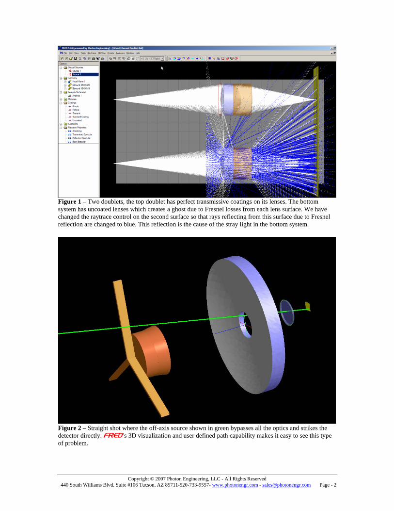
Stray Light is a problem in almost any opto-mechanical or illumination system. Reducing or eliminating Stray Light is possible by blocking or moving components, painting surfaces or applying coatings on optical components. In this note we will define terms to define what stray light is and how to use FRED to analyze and reduce stray light problems. 1. What is Stray Light Stray light is simply unwanted noise (light) that is added by either opto-mechanical structure, out of field sources, non-perfect optical components or through thermal emission in an optical or illumination system. It is this unwanted noise that FRED excels in finding and by using its virtual prototyping analysis capability helps us remove it. Stray light in imaging systems can come from a variety of sources, they are listed below. Ghost Images Ghost images are so called because they are out-of-focus or ghostly-looking images of bright sources of light.(1) Ghost images are caused by reflections from lens surfaces. To cause a ghost, light must reflect an even number of times from lens surfaces. There are two-reflection ghosts, four-reflection ghosts, etc. Optical systems consisting of only first-surface mirrors (a Cassegrain telescope, for example) do not suffer from ghost images. The sun causes ghost images in a photograph if it is in or near the field of view being photographed. Automobile headlights and streetlights cause stray light in a nighttime photograph. If the bright source is small, each ghost takes on the shape of the aperture stop of the optical system. A good ghost image example is shown in Figure 1 where one doublet has perfectly coated lenses and the second system has uncoated lenses. A diverging 21 by 21 grid of rays was traced to fill the first lens in each system. “Straight shots” Straight shots can occur for example in a Cassegrain-type system when the central obstruction is too large and/or the telescope tube is too short. Light from outside the field of view can enter the telescope, travel past the secondary mirror, through the hole in the primary mirror, and strike the focal plane directly as stray light. This type of stray light can be a disaster if sunlight is allowed to enter the telescope as shown in Figure 2.


Figure 1 – Two doublets, the top doublet has perfect transmissive coatings on its lenses. The bottom system has uncoated lenses which creates a ghost due to Fresnel losses from each lens surface. We have changed the raytrace control on the second surface so that rays reflecting from this surface due to Fresnel reflection are changed to blue. This reflection is the cause of the stray light in the bottom system.

Figure 2 – Straight shot where the off-axis source shown in green bypasses all the optics and strikes the detector directly. FRED’s 3D visualization and user defined path capability makes it easy to see this type of problem.


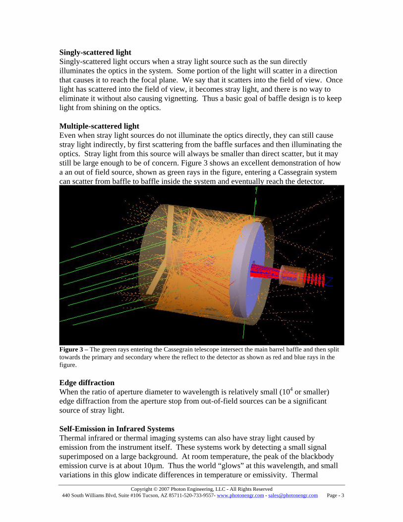
Singly-scattered light Singly-scattered light occurs when a stray light source such as the sun directly illuminates the optics in the system. Some portion of the light will scatter in a direction that causes it to reach the focal plane. We say that it scatters into the field of view. Once light has scattered into the field of view, it becomes stray light, and there is no way to eliminate it without also causing vignetting. Thus a basic goal of baffle design is to keep light from shining on the optics. Multiple-scattered light Even when stray light sources do not illuminate the optics directly, they can still cause stray light indirectly, by first scattering from the baffle surfaces and then illuminating the optics. Stray light from this source will always be smaller than direct scatter, but it may still be large enough to be of concern. Figure 3 shows an excellent demonstration of how a an out of field source, shown as green rays in the figure, entering a Cassegrain system can scatter from baffle to baffle inside the system and eventually reach the detector.

Figure 3 – The green rays entering the Cassegrain telescope intersect the main barrel baffle and then split towards the primary and secondary where the reflect to the detector as shown as red and blue rays in the figure. Edge diffraction When the ratio of aperture diameter to wavelength is relatively small (104 or smaller) edge diffraction from the aperture stop from out-of-field sources can be a significant source of stray light. Self-Emission in Infrared Systems Thermal infrared or thermal imaging systems can also have stray light caused by emission from the instrument itself. These systems work by detecting a small signal superimposed on a large background. At room temperature, the peak of the blackbody emission curve is at about 10µm. Thus the world “glows” at this wavelength, and small variations in this glow indicate differences in temperature or emissivity. Thermal


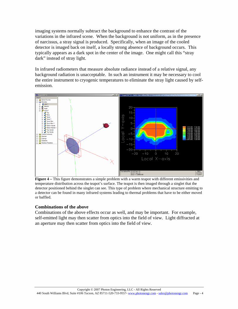
imaging systems normally subtract the background to enhance the contrast of the variations in the infrared scene. When the background is not uniform, as in the presence of narcissus, a stray signal is produced. Specifically, when an image of the cooled detector is imaged back on itself, a locally strong absence of background occurs. This typically appears as a dark spot in the center of the image. One might call this “stray dark” instead of stray light. In infrared radiometers that measure absolute radiance instead of a relative signal, any background radiation is unacceptable. In such an instrument it may be necessary to cool the entire instrument to cryogenic temperatures to eliminate the stray light caused by self-emission.

Figure 4 – This figure demonstrates a simple problem with a warm teapot with different emissivities and temperature distribution across the teapot’s surface. The teapot is then imaged through a singlet that the detector positioned behind the singlet can see. This type of problem where mechanical structure emitting to a detector can be found in many infrared systems leading to thermal problems that have to be either moved or baffled. Combinations of the above Combinations of the above effects occur as well, and may be important. For example, self-emitted light may then scatter from optics into the field of view. Light diffracted at an aperture may then scatter from optics into the field of view.


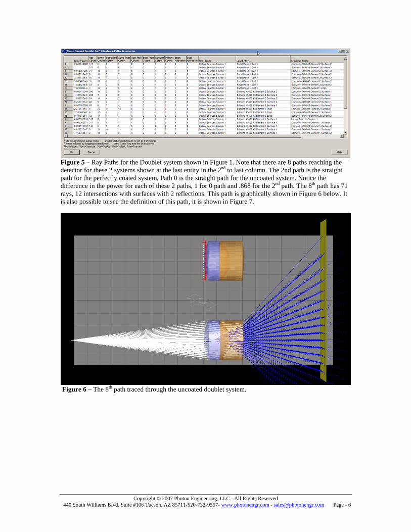
2. How does FRED visualize Stray Light? To track stray light there are several methods. The first is to create a source and ray trace it though the optical system. The second way is to ray trace backwards from the detector through the system. It is extremely important to be able to visualize stray light paths using almost any 3D ray tracing software program. Photon Engineering uses a product called FRED to show where stray light occurs. Reflected and refracted rays are only a partial part of the problem, turning scattering on is another problem altogether. 3. How does FRED create geometry? System geometry can be created directly in FRED through the simple to use graphical interface, imported from IGES or STEP CAD formats and optical design programs, or converted from ASAP output text files. The program has many options to create surfaces including standard planes, conics, cylinders, ellipsoids, hyperboloids, toroids, polynomial surfaces, Zernike, Nurb, Meshed, revolved curves, extruded curbs, composite curves, splines and user-defined surfaces. A selection of these surface created in FRED can be seen in the figures 1 and 2. Since FRED has a multiple document user interface, components may be cut, copied, and pasted between documents. Entities may be logically arranged into hierarchies of assemblies, subassemblies, elements, etc. that correspond to the physical layout of the system; each can be located relative to any arbitrary coordinate system. Any surface may be trimmed (sliced) by any implicit surface, or by an aperture collection curve, which is defined below. 4. How does FRED keep track of Ray Paths? FRED has the capability to do an advanced ray trace that keeps track of all the paths for all rays traced in a system. Figure 5 shows a list of ray paths for the two doublet lenses shown in Figure 1. This ray history is a complete report of the power for each path, the number of rays that followed that path, how they reached the last entity (Focal plane in this example) and how many surfaces they went through (Event Count). It is also possible to take any ray trace path and copy it to a user defined path list (select the path, right mouse click on the path and then select the option to copy this path to the user-defined path list). This path will now show up as an optional path in the advanced ray trace as one of the ray methods to use. It is then possible to do spot diagrams irradiance spread functions on only this path. It is by using this method that it is possible to see how much power each of the ghosting, straight shot, single or multiple scatter paths contribute versus the signal path.


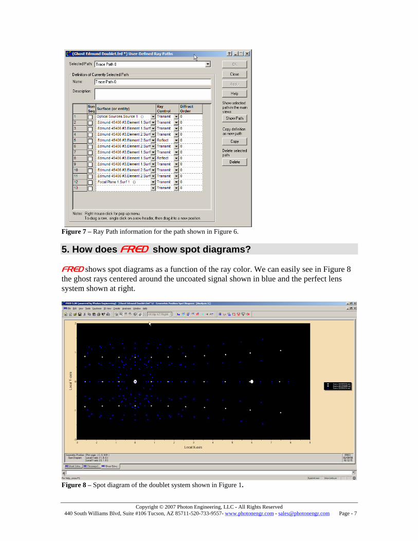
Figure 5 – Ray Paths for the Doublet system shown in Figure 1. Note that there are 8 paths reaching the detector for these 2 systems shown at the last entity in the 2nd to last column. The 2nd path is the straight path for the perfectly coated system, Path 0 is the straight path for the uncoated system. Notice the difference in the power for each of these 2 paths, 1 for 0 path and .868 for the 2nd path. The 8th path has 71 rays, 12 intersections with surfaces with 2 reflections. This path is graphically shown in Figure 6 below. It is also possible to see the definition of this path, it is shown in Figure 7.

Figure 6 – The 8th path traced through the uncoated doublet system.


Figure 7 – Ray Path information for the path shown in Figure 6. 5. How does FRED show spot diagrams? FRED shows spot diagrams as a function of the ray color. We can easily see in Figure 8 the ghost rays centered around the uncoated signal shown in blue and the perfect lens system shown at right.

Figure 8 – Spot diagram of the doublet system shown in Figure 1.


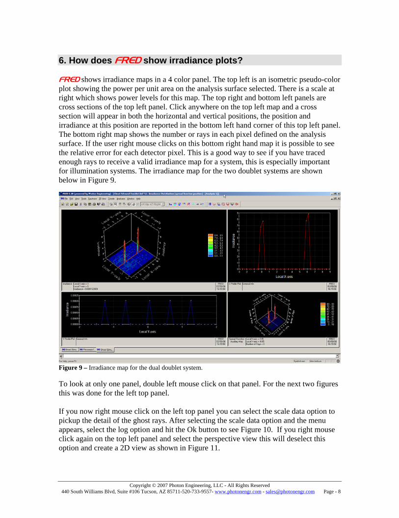
6. How does FRED show irradiance plots? FRED shows irradiance maps in a 4 color panel. The top left is an isometric pseudo-color plot showing the power per unit area on the analysis surface selected. There is a scale at right which shows power levels for this map. The top right and bottom left panels are cross sections of the top left panel. Click anywhere on the top left map and a cross section will appear in both the horizontal and vertical positions, the position and irradiance at this position are reported in the bottom left hand corner of this top left panel. The bottom right map shows the number or rays in each pixel defined on the analysis surface. If the user right mouse clicks on this bottom right hand map it is possible to see the relative error for each detector pixel. This is a good way to see if you have traced enough rays to receive a valid irradiance map for a system, this is especially important for illumination systems. The irradiance map for the two doublet systems are shown below in Figure 9.

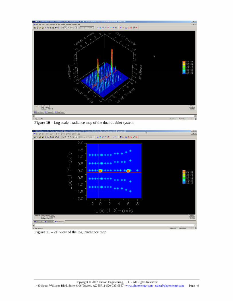
Figure 9 – Irradiance map for the dual doublet system. To look at only one panel, double left mouse click on that panel. For the next two figures this was done for the left top panel. If you now right mouse click on the left top panel you can select the scale data option to pickup the detail of the ghost rays. After selecting the scale data option and the menu appears, select the log option and hit the Ok button to see Figure 10. If you right mouse click again on the top left panel and select the perspective view this will deselect this option and create a 2D view as shown in Figure 11.


Figure 10 – Log scale irradiance map of the dual doublet system

Figure 11 – 2D view of the log irradiance map


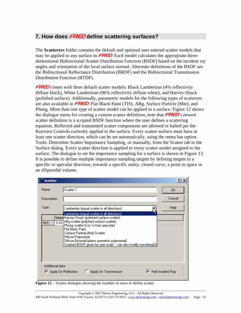
7. How does FRED define scattering surfaces? The Scatterers folder contains the default and optional user entered scatter models that may be applied to any surface in FRED. Each model calculates the appropriate three-dimensional Bidirectional Scatter Distribution Function (BSDF) based on the incident ray angles and orientation of the local surface normal. Alternate definitions of the BSDF are the Bidirectional Reflectance Distribution (BRDF) and the Bidirectional Transmission Distribution Function (BTDF).

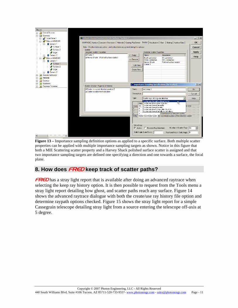
FRED comes with three default scatter models: Black Lambertian (4% reflectivity diffuse black), White Lambertian (96% reflectivity diffuse white), and Harvey-Shack (polished surface). Additionally, parametric models for the following types of scatterers are also available in FRED: Flat Black Paint (TIS), ABg, Surface Particle (Mie), and Phong. More than one type of scatter model can be applied to a surface. Figure 12 shows the dialogue menu for creating a custom scatter definition, note that FRED’s newest scatter definition is a scripted BSDF function where the user defines a scattering equation. Reflected and transmitted scatter components are allowed or halted per the Raytrace Controls currently applied to the surface. Every scatter surface must have at least one scatter direction, which can be set automatically, using the menu bar option Tools: Determine Scatter Importance Sampling, or manually, from the Scatter tab in the Surface dialog. Every scatter direction is applied to every scatter model assigned to the surface. The dialogue to set the importance sampling for a surface is shown in Figure 13. It is possible to define multiple importance sampling targets by defining targets in a specific or specular direction, towards a specific entity, closed curve, a point in space or an ellipsoidal volume.

Figure 12 – Scatter dialogue showing the number of ways to define scatter


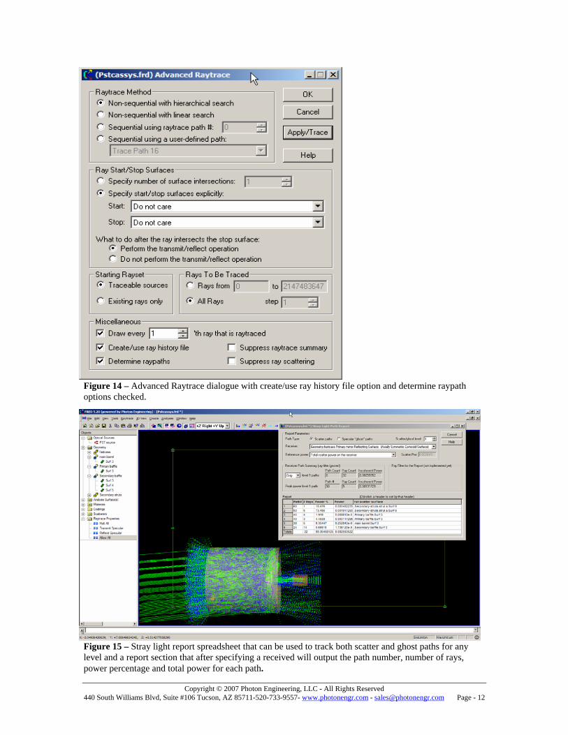
Figure 13 – Importance sampling definition options as applied to a specific surface. Both multiple scatter properties can be applied with multiple importance sampling targets as shown. Notice in this figure that both a MIE Scattering scatter property and a Harvey Shack polished surface scatter is assigned and that two importance sampling targets are defined one specifying a direction and one towards a surface, the focal plane. 8. How does FRED keep track of scatter paths? FRED has a stray light report that is available after doing an advanced raytrace when selecting the keep ray history option. It is then possible to request from the Tools menu a stray light report detailing how ghost, and scatter paths reach any surface. Figure 14 shows the advanced raytrace dialogue with both the create/use ray history file option and determine raypath options checked. Figure 15 shows the stray light report for a simple Cassegrain telescope detailing stray light from a source entering the telescope off-axis at 5 degree.


Figure 14 – Advanced Raytrace dialogue with create/use ray history file option and determine raypath options checked.

Figure 15 – Stray light report spreadsheet that can be used to track both scatter and ghost paths for any level and a report section that after specifying a received will output the path number, number of rays, power percentage and total power for each path.


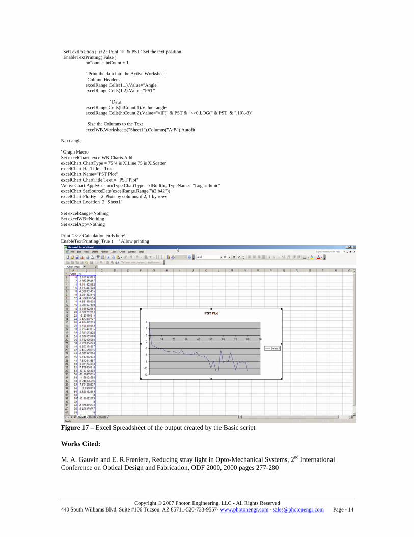
9. How does FRED iterate across multiple point sources to create a PST power per angle output? FRED has a built-in compiled Basic scripting language. Almost all Graphical User Interface (GUI) commands are available from the Visual Basic scripting language. FRED also has Automation Client and Server capability which can be called or call other Automation enabled programs like Excel. So it is possible to define multiple off-axis sources and the use For Next loops in the FRED Basic scripting language to do azimuth and zenith scans around a system to create a Point Source Transmittance curve. The Log PST curve for the Cassegrain system shown in Figure 15 is shown in Figure 17. Notice that the BASIC script in Figure 16 calls Excel to do the PST plotting in Log space which is shown Figure 17. Figure 16 – FRED Basic Script to create a Log PST plot in Excel 'PST script example showing changing incoming ray directions For analysis 'declarations Dim op As T_OPERATION Dim pRay As T_RAY Dim PST As Double Dim XlRows As Constant Dim xlXYScatterLinesNoMarkers As Long '' Connect to Excel ' OBjects to be used Dim excelApp As Object Dim excelWB As Object Dim excelRange As Object Dim excelChart As Object ' Excel Object Setup Set excelApp=CreateObject("Excel.Application") Set excelWB=excelApp.Workbooks.Add Set excelRange=excelWB.ActiveSheet.Cells(1,1) ' Show Excel excelApp.Visible=True htCount=1 'find source node, for the Cassys file this is the PST source, change as needed node = FindName( "PST source" ) Print "found PST source at node " & node 'find detector node, for the Cassys file this is the detector array, change as needed detNode = FindFullName( "Geometry.fastcass.dewar.FPA.detector array" ) Print "found detector at node " & detNode 'Print out column headers i = GetTextCurCol : j = GetTextCurRow SetTextPosition j, i+3 : Print "PST" EnableTextPrinting( False ) ' No printing 'Specify the detector area for the system, for cassys is is rectangular .125 in radius detArea = ( 2 * 0.125 )^2 'Loop to do the PST at every 2 degrees up to 80, change as needed For angle = 0 To 80 Step 2 SetSourceDirection node, 0, Tan( angle * .017453), 1 Update DeleteRays 'Delete rays for subsequent loops CreateSources ' Make sources TraceExisting 'Draw ' Trace (and optionally draw) the rays 'PST calculation PST = GetSurfIncidentPower ( detNode ) ' Get Power On Detector PST = PST * Cos( angle * .017453) / detArea ' Calculate PST EnableTextPrinting( True ) Print "PST at " & angle & " degrees = ;" ' Print out PST header to the output window i = GetTextCurCol : j = GetTextCurRow ' Get which row and column text cursor is on


SetTextPosition j, i+2 : Print "#" & PST ' Set the text position EnableTextPrinting( False ) htCount = htCount + 1 '' Print the data into the Active Worksheet ' Column Headers excelRange.Cells(1,1).Value="Angle" excelRange.Cells(1,2).Value="PST" ' Data excelRange.Cells(htCount,1).Value=angle excelRange.Cells(htCount,2).Value="=IF(" & PST & "<>0,LOG(" & PST & ",10),-8)" ' Size the Columns to the Text excelWB.Worksheets("Sheet1").Columns("A:B").Autofit Next angle ' Graph Macro Set excelChart=excelWB.Charts.Add excelChart.ChartType = 75 '4 is XlLine 75 is XlScatter excelChart.HasTitle = True excelChart.Name="PST Plot" excelChart.ChartTitle.Text = "PST Plot" 'ActiveChart.ApplyCustomType ChartType:=xlBuiltIn, TypeName:="Logarithmic" excelChart.SetSourceData(excelRange.Range("a2:b42")) excelChart.PlotBy = 2 'Plots by columns if 2, 1 by rows excelChart.Location 2,"Sheet1" Set excelRange=Nothing Set excelWB=Nothing Set excelApp=Nothing Print ">>> Calculation ends here!" EnableTextPrinting( True ) ' Allow printing

Figure 17 – Excel Spreadsheet of the output created by the Basic script Works Cited: M. A. Gauvin and E. R.Freniere, Reducing stray light in Opto-Mechanical Systems, 2nd International Conference on Optical Design and Fabrication, ODF 2000, 2000 pages 277-280

Documents

1. What is Stray Light - Photon Engineeringphotonengr.com/.../uploads/2010/10/ApplicationNote_StrayLight.pdf · Stray Light Application Note Stray Light is a problem in almost any