NASA

Technical Memorandum 106109

/

AVSCOM

Technical Report 92-C-022

Incompressible Spectral-Element MethodDerivation of Equations

Russell G. DeAnna

Vehicle Propulsion Directorate

U.S. Army Research Laboratory

Lewis Research Center

Cleveland, Ohio

(NASA-TM-106IO9) INCOMPRESSIBLESPECTRAL-ELEMENT METHOD: DERIVATION

OF EQUATIONS (NASA) 88 D

N93-26554

Unclas

April 1993 G3/34 0160303

N/ AA_A_ Ri,T

https://ntrs.nasa.gov/search.jsp?R=19930017365 2019-05-16T14:04:32+00:00Z

INCOMPRESSIBLE SPECTRAL-ELEMENT METHOD---DERIVATION OF EQUATIONS

Russell G. DeAnna

Vehicle Propulsion Directorate

U.S. Army Research LaboratoryLewis Research Center

Cleveland, Ohio 44135

ABSTRACT

A fractional-step splitting scheme breaks the full Navier-Stokes equations

into explicit and implicit portions amenable to the calculus of variations.

Beginning with the functional forms of the Poisson and Helmholtz equations, we

substitute finite expansion series for the dependent variables and derive the

matrix equations for the unknown expansion coefficients. This method employs a

new sphtting scheme which differs from conventional three-step (non-hnear,

pressure, viscous) schemes. The non-linear step appears in the conventional,

explicit manner, the difference occurs in the pressure step. Instead of solving for

the pressure gradient using the non-linear velocity, we add the viscous portion of

the Navier-Stokes equation from the previous time step to the velocity before

solving for the pressure gradient. By combining this "predicted" pressure

gradient with the non-linear velocity in an explicit term, and the Crank-

Nicholson method for the viscous terms, we develop a Helmholtz equation for the

final velocity.

LIST OF SYMBOLS

a = value of non-homogeneous essential boundary condition

g = value of non-homogeneous natural boundary condition

A = cross-sectional area

dA = differential surface area vector

B0 = 23112, coefficient used in Adams-Bashforth method

B I =-16/12, coefficient used in Adams-Bashforth method

B2 = 5/12, coefficient used in Adams-Bashforth method

Brgc = coefficients

(Cij)aebc = coefficients

Dn = Legendre collocation derivative of order n

Dij = derivative of expansion polynomial j evaluated at node i

ex, ey, e.z = unit vectors in the direction of the coordinate axes

f = body force vector

E = total number of elements

M = moment vector

F = __rn,1, also represents a force vector

J[P] = a functional depending on P

L = periodic length of domain

L2 = square-integrable function

Lk(x) = Legendre polynomial

it, jt, kt = the maximum number of nodes in the r, s, t directions

respectively

In = a system of interpolating polynomials of order n

Ipe = surface integral for side number p and element number e

_e = total surface integral for element number e

[J] = Jacobian matrix for the transformation between coordinate systems

n -- surface unit normal vector

s = surface unit tangent vector

R = position vector

p = pressure

pi(x) -- infinite sequence of orthogonal functions

p(x), q(x), w(x) = functions in Sturm-LiouviUe equation

P = pip + _V-V, dynamic pressure

Pn - a system of orthogonal polynomials of degree n

S - an infinite system of orthogonal polynomials

t -- time

At - time-step size

t(n) = force per unit area on a surface with unit normal n

ui = discrete expansion coefficient for the infinite series

_i = discrete expansion coefficient for the finite series

V -- velocity vector

= velocity after the non-linear step

= velocity after the explicit viscous step

= velocity after the pressure step

_r = corrected velocity after the explicit viscous step

Vout = average outflow velocity correction

U, V, W = x, y, z velocities respectively

wi = weight function, integral of the expansion polynomial over domain

x, y, z = coordinates in global or physical space

xr = partial derivative of the global co-ordinate x with respect to the local

co-ordinate r

r, s, t = coordinates in local or transformed space

rx = partial derivative of the local co-ordinate r with respect to the global

co-ordinate x

Greek and other Symbols

- constantin homogeneous boundary condition

= constant in homogeneous boundary condition

7 = coefficient in expansion polynomial relationships

6 - differential of a quantity

_ij "- Kronecker delta

_i(x) = a combination of Legendre polynomials

= infinitesimal quantity

_ijk "- alternating tensor

f_ = domain under consideration

8f/= boundary of domain under consideration

= nusn

V

= eigenvalue in Sturm-LiouviUe equation

A = matrix of coefficients representing A in the expression

11 = matrix of coefficients representing b in the expression

p = fluid density

a = stress tensorm

-- element surface area

aij = i, j component of the stress tensor

X -- moment arm

¥ = element volume

# = fluid viscosity

u = fluid kinematic viscosity

= _xex + _yey + _zez, vorticity vector

Ax=b

Ax=b

4

Subscripts

0 = initial value

® = free-stream value

e = element number

n = direction normal to the surface

s = direction tangential to the surface

ijk = co--ordinate system indices

in = value at inlet

out = value at outlet

wall -'- value at wall

x,y,z = streamwise, vertical, and spanwise values respectively, may also

refer to partial derivatives with respect to the global co-ordinates x, y, z

Superscripts

n --- time step number

e - element number

1,2,s,4, s, 6 = element side numbers

INTRODUCTION

The new splitting scheme, developed by Wessel (1992), contains variations

on the original three-step splitting method proposed by Korczak and Patera

(1986). In the previous scheme, the non-linear, pressure, and viscous terms in the

incompressible Navier-Stokes equations appear in separate fractional steps. By

introducing intermediate velocities, solutions of these equations yield,

consecutively, a velocity field based on the non-I/near, the pressure and non-

linear, and the viscous, pressure, and non-linear terms. The final step producing

the true velocity field.

\

5

The velocity field resulting from the non-linear step satisfies no boundary

conditions nor the incompressibility constraint. This velocity field supplies the

forcing function for the Poisson equation for pressure after applying the

divergence operator to the pressure step. The intermediate velocity contained in

the pressure step must satisfy the divergence free constraint, thus it vanishes

from the Poisson equation for pressure. Instead of solving a second-order Poisson

equation for pressure, a first-order equation for pressure gradient is solved using

methods from the calculus of variations-the velocity field follows directly from

the pressure step. Inviscid boundary conditions on velocity determine the

pressure boundary conditions; hence, errors of 0(_t) occur near solid boundaries.

Finally, the viscous step employs a Crank-Nicholson scheme yielding a Helmholtz

equation with a forcing function determined by the velocity after the pressure

step. Once again a variational form of the governing second-order differential

equation reduces the order by one. The velocity must satisfy the full, viscous

boundary conditions; however, it does not satisfy the incompressibility

constraint.

The new method varies slightly from the old. Instead of solving for the

pressure gradient using the non-linear velocity, we include the viscous term from

the previous time step. Thus, the forcing function appearing in the Poisson

equation for pressure contains contributions from both non-linear and viscous

terms. The resulting pressure gradient is not solved for the velocity after the

pressure step; instead, it, along with the velocity from the non-linear step, and a

Crank-Nicholson method for the viscous terms, produce a Helmholtz equation for

the full velocity. The boundary conditions and solution procedure remain

identical to the original method. The boon comes from including the viscous

6

terms in the pressuregradient prediction, resulting in a quicker solution of the

pressure step.

7

CHAPTER I

SPECTRAL APPROXIMATION

1.1SpectralTheory

The expansion of a function u in terms of an infinite sequence of

orthogonal functions {Pi}, u = _i---_ fiiPi, underlies many numerical methods

of approximation. The most familiar approximation results apply to periodic

functions expanded in Fourier series. In this case, the i-th coefficient of the

expansion decays faster than any inverse power of i for smooth functions with

periodic derivatives. The rapid decay of the coefficients implies that the Fourier

series truncated after a few terms represents a good approximation to the

function. This characteristic refers to the "spectral accuracy" of the Fourier

method.

Spectral accuracy for smooth but non-periodic functions occurs with the

proper choice of expansion functions. Not all orthogonal expansion functions

provide high accuracy; however, the eigenfunctions of a singular Sturm-Liouville

operator allow spectral accuracy in the expansion of any smooth function, with

no a priori restriction on the boundary behavior.

The expansion in terms of an orthogonal system introduces a linear

transformation between u and the sequence of its expansion coefficients {fii},

called the finite transform of u between physical space and spectral space. Since

the expansion coefficients depend on all the values of u in physical space, they

rarely get computed exactly; instead, a finite number of approximate expansion

coefficients result from using the values of u at a finite number of selected

points-the nodes. This procedure defines a discrete transform between the set of

values of u at the nodes and the set of approximate, or discrete coefficients.

With a proper choice of nodes and expansion functions, the finite series defined

by the discrete transform represents the interpolation of u at the nodes.

Maintaining spectral accuracy when replacing the finite transform with the

discrete transform allows use of the interpolation series instead of the truncated

series in approximating functions.

1.2 Sturm-Liouvine Problems

The importance of Sturm-Liouvil]e problems for spectral methods lies in the

fact that the spectral approximation of the solution of a differential problem

often occurs as a finite expansion of eigenfunctions of a suitable Sturm-Liouville

problem. The general form of the Sturm-Liouville problem satisfies

d , du_-_]xtp_ } + qu = _wu in fl E (-1,1/. (1.2.1/

The real-valued functions, p(x), q(x), and w(x), must behave properly: p(x)

must be continuously differentiable, strictly positive in (-1,1) and continuous at

x=*l; q(x) must be continuous, non-negative and bounded in (-1,1); the

weight function w(x) must be continuous, non-negative and integrable over

(-1,1/. The Sturm-Liouville problems of interest in spectralmethods allow the

expansion of an infinitely smooth function in terms of their eigenfunctions while

guaranteeing spectral accuracy.

1.30rthogonal Systems of Polynomials

Consider the expansion of a function in terms of a system of orthogonal

polynomials of degree less than or equal to n, denoted by Pn- Assume

{Pk}k--0,1.-. represents a system of algebraic polynomials (with degree of pk=k)

mutually orthogonal over the interval (-1,1) with respect to a weight function

w(x). The orthogonality condition requires

1

./_ - - - - --{'ipk(x)pm(x)w(x)dx=0 whenever rusk. (1.3.2)

9

The formal seriesof a square-integrable function,

system {Pk} appears as

when the expansion coefficients

C9

Su = k_0UkPk(X),

Uk satisfy

1 !

- ll ll2 -lu(x)pk(x)w(x)dx"

uEL_(--1,1)_:,

For an integer n>O, the truncated series of u of order n appears as

n

integration formulas on the interval [-1,1]. Let

(n+l)-th orthogonal polynomial Pn,l and let

the linear system given by

in terms of the

(1.3.3)

(1.3.4)

Pnu - k_=oUkPk(X). (1.3.,5)

1.4 Gauss-Lobatto Quadratures and Discrete Polynomial Tmndorms

Expanding any u(x)EL2(-1,1) in terms of the coefficients Uk, called the

continuous ezpaasion, depends on the known function u(x). With u(x) is not

known a priori, a discrete expansion for u(x)-which depends on the values at the

nodes-must suffice.

A close relation exists between orthogonal polynomials and Gauss-Lobatto

Xo,...,Xn equal the roots of the

Wo,...,Wn equal the solution of

0 < k < n, (1.4.1)

w(x) equals the weight function associated with the Sturm-LiouviUe

j = O,...,n, and

n I

j_0P(xjlw j -- f.,p(xlw(x)dx, (1.4.2)

The positive numbers wj are called "weights" (see Canuto

This version of Gauss integration produces roots,

where

problem, Wj>0 for

hold for all PEP2n+I.

et. al.(1988) for proof).

:_Identifying the function u(x) as "square integrable" on the given domainrequires Jlu(x)),2dx < ®.

10

corresponding to the collocationpoints,which appear in the interiorof (-i,i).

Since boundary conditionsrequireone or both end points,a generalized Gauss

integrationformula must include these points.

The Ganss-Lobatto formula considers

q(x) = pn.1(x) + apn(X) + bpn-1(x), (1.4.3)

with a and b chosen so that q(-1)=q(1)=0. For a given weight function

w(x) and corresponding sequence of orthogonal polynomials Pk, k=0, i, 2,...

we denote by x0,...,xn the nodes of the n+l point integration formula of

Gauss-Lobatto type, and by w0,...,Wn the corresponding weights.

In a collocation method the fundamental representation of a smooth

function u on (-1,1) appear in terms of its values at the discrete Gauss-

Lobatto points. Approximate derivatives of the function occur by analytic

derivatives of the interpolating polynomial. The interpolating polynomial,

denoted by Inu, belongs in the set Pn and satisfies

Since (1.4.4)

by

InU(Xj) = U(Xj) 0 < j < n. (1.4.4)

represents a polynomial of degree n, it admits an expression given

n

InU-- k_oUkPk(X). (1.4.5)

Since the interpolating polynomial must satisfy the function exactly at the nodes,

we get

n

U(Xj) ----k_0UkPk(Xj), (1.4.6)

equal the discrete polynomial or e_ar_ion coefficients of u. The

(1.4.7)

where _k

inverse relationship satisfies

1 u(xj)pk(xj)wj,

11

{u(xj)} and spectra] space

associated with the weights

1.5 Legend_e Polynomials

where the coefficients7k equal

n

"Fk-" j_ffi0p_ (xj)wj. (1.4.8)

Equations (1.4.6) and (1.4.7) enabling transforms between physical space

{uk} are called the discrete polynomial tra_sforms

w0,...,Wn and the nodes x0,...,Xn.

A collection of the essential features ofLegendre polynomials appears

below. The Legendre polynomials {Lk(x), k - 0, 1,...,} equal the eigenfunctions

of the singular Sturm-LiouvilIe problem given by

_:[(1--x2)_i_Lk(X)]+ k(k + 1)Lk(x)= 0, (1.5.1)

which equals (1.1.1) with p(x)=l-x _, q(x)=0 and w(x)=l. By normalizing

Lk(x) so that Lk(1)--l,the Legendre polynomials satisfy

d kL],(x) - 1! _k (x 2- 1) k

and _epresent the solutionto (1.5.i) with boundary conditions (1.5.5).

polynomials also satisfythe recurrence relation,expressed as

Lko(X) 2k + l xLk(x) k: 1 -- _ Lk-l(X),

where L0(x):l and Ll(x)--x,

(1.5.2)

These

(1.5.3)

ILk(x)l < I, --l<x_. 1,

Lk("l) -- (*I)},

IL'k(X) l <½k(k+l), -1<x__1,

L'k(4"l) = (4"1)k ½k(k "t"1),

/.' L_(x)dx -- (k + ½)",and

along with the property that Lk(x) iseven if k iseven, and odd if k isodd.

The continuous expansion of any ueL2(-1,1) in terms of the Legendre

(1.5.4)

(I.5.S)

(I.5.S)

(1.5.7)

(1.S.8)

12

polynomials appears as

U(X) = _ fikLk(X I. (1.5.9)k--O

Multiplying both sides by Lj(x) and integrating from x=- I to x=l, gives

1 k=O

where w(x)=l according to (1.3.2 I. Using the orthogonal properties of the

Legendre polynomials and (1.5.81 gives

I ,i I

fij = (j "-I-_)J.l.u(x)Lj(x)cbr-. 0.5.11)

The Legendre polynomials may appear directly as the expansion functions of

(1.5.9 / or as a combination of Legendre polynomials which satisfy

j(xi)= 6ij,

where _x) equals

1 (i - x21 di_Ln(xl. "(1.5.13)CJCX)=n(n+l)Ln(xjix- xj

This later form allows simpler implementation. The nodes {xj}, j-1,...,n-1,

equal the zeros of d[_Ln(x), with x0=- 1, and xn--1. The qua&ature weights,

shown in (1.4.21, satisfy

n

k_O_J(XkIW k -- /_: _j(x)w(x)dx. (1.5.14)

Since the Legendre polynomials correspond to w(x)=l, and the expansion

polynomials satisfythe relation _j(Xk)--bkj, (1.5.14) reduces to

Or

'_ _kjWk- f.l 1 _j(x)dx (1.5.15)k=O

Insertingthe expression for the expansion polynomial,

integration

(1.5.16)

(1.5.13),gives after

13

2 1

wj - n(n + I)_(_ ' j= 0,...,n

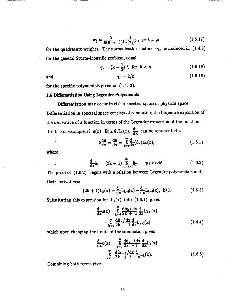
for the quadrature weights. The normalization factors "p,,

for the general Sturm-Liouville problem, equal

_=(k+½) -I, for k<n

and "Yn= 2/n.

for the specific polynomials given in (1.5.13).

1.6 Differentiation Using Legendre Polynomials

(1.5.17)

introduced in (1.4.8)

(1.5.18)

(1.5.19)

Differentiation may occur in either spectral space or physical space.

Differentiation in spectral space consists of computing the Legendre expansion of

the derivative of a function in terms of the Legendre expansion of the function

itself. For example, if u(x)=_k:0 _kLk(x), du_-_ can be represented as

where

S_ du _0_-(= -- l_tk)Lk(X),g_ k

The proof of (1.6.2)

their derivatives:

(2k÷Substituting this expression for Lk(x) into (1.6.1) gives

" dtlk / (ix _[_Lk_U(X)---- k_.O 2k + 1

® d_k / dx _]_L-- _ k-l(X)k--0 2k + 1

which upon changing the limits of the summation gives

(1.6.1)

®

_Uk -- (2k ÷ 1) p_k,Z_p, p÷k odd. (1.6.2)

begins with a relation between Legendre polynomials and

_]_u(x) = _, d_k-,/dx _Lk(x)k=x2k - 1

® d_k,I/dxd , r__--k_=.12k + 3 _[_'-k_,X].

Combining both terms gives

k>O. (1.6.3)

(1.6.4)

(1.6.5)

14

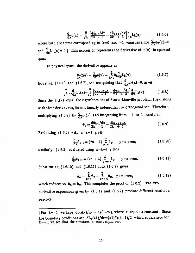
where both the terms corresponding to k=0 and -i vanishes since

and _[_L-1(x)= 0.:_This expressionrepresentsthe derivativeof u(x)

space.

In physical space,the derivativeappears as

Equating

Since the

(1.6.6)

_I_L0(x)=0

in spectral

_-(Su) _u(x) ® d-- = __ fk:;r=Lk(X).kffi0 u.A

(1.6.6) and (1.6.7),and recognizingthat _L0(x)--0, gives

® d ® rdfk-l/dX dfk. l/dx]d . ,_,fk-___-__Lk(X)----_k--1 ax k=lL2k - 1 2k % 3 J_ ''ktxj"

Lk(x)

(1.6.7)

(1.6.8)

equal the eigenfunctionsof Sturm-Liouville problem, they, along

with their derivatives, form a linearly independent or orthogonal set. Therefore,

_]_Lj(x) and integrating from -1 to 1 results inmultiplying (1.6.8) by

fk = dfik-l/dX_ dfk. l ldx (1.6.9)2k - 1 2k + 3 "

Evaluating (1.6.2) with n=k+l gives

df ®-= (2n-1)Z__Up,

similarly, (1.6.2) evaluated using n=k-i yields

®

_]Efn,,-" (2n -I- 31 pZ=n, fi p,

p+n even; (1.6.10)

p+n even.

Substituting (1.6.10) and (1.6.11) into (1.6.9) gives

® ®

fin -- _ Up -- _n+2Up, p+n even,p=n p

which reduces to fin - fin- This completes the proof of (1.6.2).

derivative expressions given by

(1.6.11)

(1.6.1) and (1.6.7)

(1.6.12)

The two

produce differentresultsin

practice:

:_For k=-i we have dL.1(x)/dx = c/(l-x2), where c equals a constant. Since

the boundary conditionsare dLk(*1)/dx=(*l)kk(k+l)/2 which equals zero for

k=-1, we see that the constant c must equal zero.

15

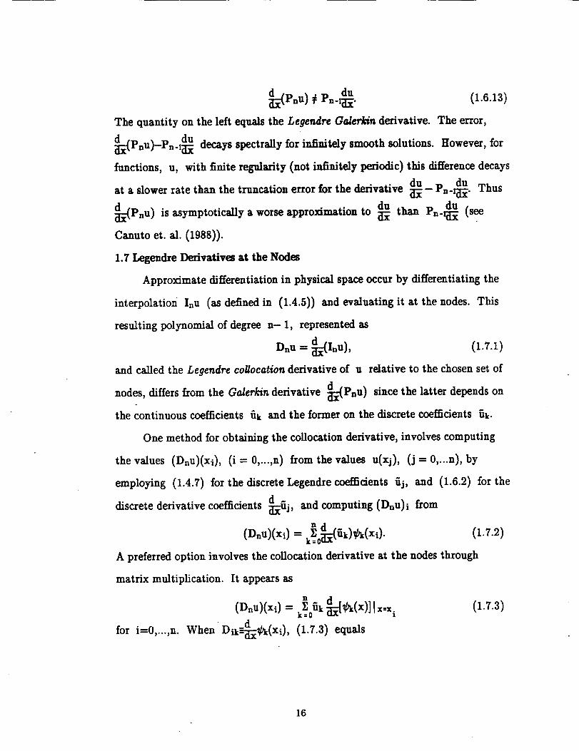
_'(Pnu) _ Pn-_. (1.6.13)

The quantity on the left equals the Legen_lre Galerkin derivative. The error,

__(p u _ p dun J- n-l_ decays spectrally for infinitely smooth solutions. However, for

functions, u, with finite regularity (not infinitely periodic) this difference decays

_[__ p duat a slower rate than the truncation error for the derivative n-r_. Thus

de p du (see_'_,Pnu) is asymptotically a worse approximation to _ than n-_

Canuto et. al. (1988)).

1.7 Legendre Derivatives at the Nodes

Approximate differentiation in physical space occur by differentiating the

interpolation InU (as defined in (1.4.511 and evaluating it at the nodes.

resulting polynomial of degree n- 1, represented as

Dnu = _'(Inul,

This

(1.7.1)

and called the Legendre collocation derivative of u relative to the chosen set of

nodes, differs from the Galerki_ derivative _-(Pnu) since the latter depends on

the continuous coefficients _k and the former on the discrete coefficients _k.

One method for obtaining the collocation derivative, involves computing

the values (Dnu)(xi), (i = 0,...,n) from the values u(xj), (j = 0,...n), by

employing (1.4.7) for the discrete Legendie coefficients _j, and (1.6.2) for the

d_.discrete derivative coefficients _ j, and computing (Dnu)i from

(Vnul(xi) - k_k-(Sk)_(xi). (1.7.2)

A preferred option involves the collocation derivative at the nodes through

matrix multiplication. It appears as

(Dnul(xiI - k_0Uk kCx)]l=r. X X I

for i=0,...,n. When'Dik=-_(xi), (1.7.31 equals

(1.7.3/

16

n

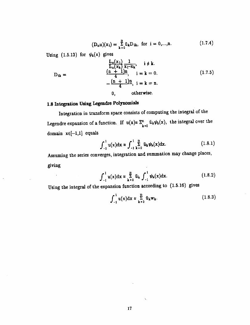
(Dnu)(xi) - kSo_kDik,= for i -- 0,...,n. (1.7.4)

Using (1.5.13) for _(x) gives

1 i_k.•Ln(Xk).X-'i-l-Xk'

(n + l)n i = k = O. (1.7.5)Dik = 4 '

_(n 4+ l)n, i=k=n.

O, otherwise.

1.8 Integration Using Legendre Polynomials

Integration in transform space consists of computing the integral of the

Legendre expansion of a function.

domain xe[-1,1] equals

If .(x)-- z" _k_(x),k=O

the integral over the

I.i*)Assuming the series converges, integration and summation may change places,

giving

1

I k=O 1

Using the integral of the expansion function according to (1.5.16) gives

(1.8.2)

__ niu(x)dx_ ]_5kwk.I k=O

(I.S.3)

17

CHAPTER II

SPECTRAL ELEMENT METHOD

2.1 Introduction

The spectral-element method, a variational procedure in which the

approximating functions depend on representing the given domain as a collection

of simple sub-domains, differs from both spectral methods and finite-element

methods in two ways: (1) pure spectral methods employ high degree

approximating functions with support defined over the entire domain, and (2)

finite-element methods use low degree approximating functions with compact

•support (i.e., a given element's approximating functions differ from zero only

within the element). Spectral-element methods exploit the advantage of high

degree functions inherent in pure spectral methods, along with the flexibility

finite-element methods provide in representing complex domains. The sub-

domains, or finite elements, equal geometrically simple shapes that permit a

systematic construction of the approximating functions. These ecumenical

functions satisfy all boundary conditions and problem data by employing

concepts of orthogonal polynomials from Sturm-Liouville theory. On an

elemental basis, the dependent variables appear as a finite sequence of the

approximation functions with coefficients representing the dependent variables at

a finite number of preselected points (i.e., nodes, whose number and location

dictates the degree and form of the approximating functions).

2.2 Partitioning of Domain

One feature of the spectral-element method distinguishing it from the pure

spectral method allows representing the given domain by a collection of sub-

domains. A subsequent transformation maps each sub-domain from the physical

18

(x,y,z) space to the local (r,s,t) space by an isoparametric mapping. The sub-

domains in local space equal simple geometries, such as cubes in three-

dimensional space. Two important features in typical geometries dictate this

mapping: first, the definition of the approximation functions from Sturm-

Liouville equations only apply to certain well-defined geometries; and second, an

arbitrary domain cannot accept a collection of simple domains without

introducing error. By defining the approximating functions element-wise, the

accuracy of the approximation improves by increasing either the number of

dements (i.e., refining the mesh) or the degree of the approximating functions.

In mathematical terms, the total domain _--[_U_3fl splits into a finite

number, E, of subsets, _e, called finite dements, such that: each l_e is closed

and non-empty; the boundary _fle of each _e is Lipschitz-continuous (no

singularities, cusps, et cetera); the intersection of any two distinct dements is

eSf; and the union _ of all dements _e equals theempty, i.e., fleNf]f-_e,

total domain, given as

E

fi -- Y' fie- (2.2.1)e--I

We could not satisfy the last property without the mapping between physical and

local space.

2.3 Spectral-Element Interpolation

By allowing the possibility that each element represents the entire domain

with the general boundary conditions of the differential equation, the essential

boundary conditions equal the values of the independent variables at the nodes,

while the natural boundary conditions get subsumed into the variational form of

the equation over the element. After assembling the elements, the boundary

values on portions of the boundaries of elements sharing the boundary of the

19

given domain are replaced by the actual specified values (imposition of boundary

conditions).

In the spectral-element method, the minimum degree of the algebraic

approximating functions depends on the order of the differential equation being

solved, and the degree of the polynomial in turn dictates the number of

interpolation points, called nodes, to be identified in the element.

The approximation functions, also called interpolation functions, depend on

interpolation of the function and possibly its derivatives at the nodes of the

element. The nodes placed along the boundary of the element un/cluely define the

element geometry. Place any additional nodes required to define the

interpolation functions at other points, either in the interior or on the boundary.

The boundary nodes also enable the connection of adjacent elements by requiring

equality of the primary degrees of freedom (i.e., variables that appear in essential

boundary condition) at nodes shared by any two elements. Thus, we cannot

accurately represent discontinuous primary variables. Such problems arise in, for

example, the study of compressible flow where shock waves contain velocity

discontinuities. These functions make poor primary variables in the spectral-

element model unless we employ special procedures during assembly.

For each _e, let Pne denote the finite-dimensional spaces spanned by

linearly independent local interpolation functions _}_=0 of the nodal points.

Over each element _eCt_ the approximation Inu e of u e equals

n

U e _ Inue --_05_(r), (2.3.1)

where the localexpansion coef_cients 5_ equal the values of ue at the

preselectednodes {r_} in the element _e. As indicatedin §1.5, the

interpolation functions satisfy

2O

_b_(rj) = _ij,

where 6ij is the Kronecker-delta function.

2.4 Connectivity (or Assembly) of Elements

(2.3.2)

As mentioned earlier, all elements contain boundary nodes defining their

geometry and allowing connection with their neighbors. The connectivity of

elements requires equal values of the primary variables in nodes common to

adjacent elements. Assembling the unique sub-domains into the entire domain, a

process known as direct stiffness, requires the identification of a universal or

global system of nodes, and a corresponding set of global expansion coefficients

for the primary variables. The resulting matrix expression relates the global

expansion coefficients to the parameters of the governing differential equation

and boundary conditions.

As indicated eaxlier, the primary variables, those associated with the

essential boundary conditions, appear as the global expansion coefficients of the

assembled matrix relation. The secondary variables appear in the natural

boundary conditions.

2.5 Isoparametric Formulation

Isoparametric schemes use the same interpolation functions to represent

both the co-ordinate mapping and the primary variables. Thus, the physical

space x maps into the local r co-ordinate system by

n

= (2.5.1)when primary variables appear as

n

Ue _ Inn e ---- Y, fie_b_l(r). (2.5.2)i:o

21

CHAPTER HI

TIME-SPLITTING SCHEME FOR THE NA IE --STOKES EQUATIONS

3.1 Governing Equations and Boundary Conditions

According to the formulation given below, the domain under consideration,

nc_ s with boundary Of/, may translate but not deform. The Navier-Stokes

equations on the closed domain,

continuity equation given by

_=f/UOfl, consist of the constant density

V-V= O, (3.1.1)

and the corresponding momentum equation expressed as

ov _Vp+ f+ _W._- + (v.v)v = p

Introducing

v,v,,v = -(v.v)v + _v(v.v)

into the momentum equation gives

aN _ v,v,v - v(pt+ _v.v) + f + w2v,YI--

(3.1.3)

(3.1.4)

in which both V and p along with the body force, f, depend on both position

in the fluid and time.

The physical boundary conditions for a given problem must allow us to

divide the entire boundary into regions associated with essential boundary

conditions (e.g., walls and inlets), natural boundary conditions (e.g., outlets and

fxee-streams), and periodicity boundary conditions. The numerical procedure

handles each of these regions separately.

The essential boundary conditions appear as

v = V.a,1 (3.1.s)

on solidwall boundaries, and

v = vi. (3.1.6)

22

on inlet boundaries.

where

and

The natural boundary condition at the outflow equals

(n-¥)V - 0, (3.1.7)

n is the outward surface normal vector, and along the free stream

n-V --- n'Vboundary (3.1.8)

n=(a-n) = 0, (3.1.9)

where __ equals the local stress tensor. Equation (3.1.9) expresses the fact that

the stress at the free stream must lie entirdy normal to the boundary. By

manipulating the pair of conditions (3.1.8) and (3.1.9) we can show that they

equal the homogeneous natural condition on velocity, (n-P)V=0, (see appendix

C). The boundary condition along periodic surfaces equals

V(x+L) = V(x), (3.1.10)

where L equals the relative position vector between the two periodic boundaries.

All of these conditions refer to velocity; pressure boundary conditions depend on

the governing equations. Finally, the initial conditions equal V(x,t=0)=V0(x)

for xEflC_ 3.

3.2 Splitting Method

In the variational solution of time-dependent problems, we represent the

dependent variables in a finite dimensional vector space. The undetermined

coefficients depend on time, while the base functions depend on spatial co-

ordinates. This leads to a two-stage approximation, both of which could employ

Variational methods. We choose to discretize the equations in space and iterate

in time, thus giving a spatial variational problem. Such a procedure,commonly

known as a semi-discrete approximation, results in a set of ordinary differential

equations in time.

23

No variational form exists for the full momentum equation; therefore, we

split it into simple forms and apply variational techniques to each portion

individually. Employing the splitting scheme followed by Wessel (1992), we

introduce intermediate velocities, V, _/', _r, and V, which allows splitting of

the momentum equation into fractional steps. The scheme employs a "predictor-

corrector" approach whereby the predicted velocity at time step n+l, which

results from sequentially computing intermediate velocities based on the non-

Linear terms, the viscous terms, and the pressure terms, determines the pressure

gradient. The corrected velocity depends on this predicted pressure gradient. A

brief explanation follows. The first, or non-linear, step appears as

•,_-.n+l _ V n _ VnxVxV n + i_,1" (3.2.1)At --

the second, or pisco_s, step equals

At -- uv_vn; (3.2.2)

and the third,or pres_re, step includes

-_ = -V(_ + ½vn'I"V n+')= -VP n.1. (3.2.3)

The velocity afterthe pressure step, _/_+i must satisfythe divergence-f_ee

constraint. By applying the divergence operator to (3.2.3),a relationship

between pressure and x_n*1 ensues. The solutionof thisPoisson equation for

pressure determines the predicted pressure gradient. Using the previously

computed velocityafterthe non-linearstep and thisnew pressure gradient,a new

velocityresultsafteradding the explicitviscousterm:

_[n,l _ _rn÷l = _vpn,1 + _vV2Vn. (3.2.4)At

We stillmust add another ½_2V to the fight-hand sideto yieldthe fullNavier-

Stokes equation. We use the Crank-Nicholson method by adding ½uV_V TM to

24

the velocity _n,1 giving an implicitviscous step appearing as

Vn,1_ _?n,1 ½w_vn*I- (3.2.5)at --

We benefit from this splitting scheme by representing the implicit viscous and

pressure steps in time-independent, elliptic form: the viscous step in the form of

Helmholtz's equation, and the pressure step as Poisson'sequation. We express

both equations in variationalform and solve them by findingthe extremum of

the corresponding functional. Some of the detailsof each of the fivesteps appear

below. The two steps containing the explicitviscousterms require no exposition.

3.3 Non-Linear Step

We solve the non-linearadvective term explicitlyusing a t_ee-step Adams-

Bashforth method given by (3.3.1)

Vat = B0(VxV=V + f)n÷ BI(V=VxV + f)n-1+ B_(V=V=V ÷ f)n-2.:_

This hyperbolic operator imposes stability conditions, in the form of a Courant-

Friedrich-Lewy number, on the scheme. Neither boundary conditions nor

continuity constraints apply to x_rn*1.

3.4 Pressure Step

The velocity after the pressure step, V, must satisfy the zero divergence

constraint. Applying the divergence operator to (3.2.2) gives

- V"a_ ,l.)= V.(_vpn,1)" (3.4.1)

Since V does not satisfythe zero divergence constraint, (3.4.1) simplifiesto

v'_rn÷l ----V-VP n*l (3.4.2)at

The boundary conditions on pressure depend on the governing equations.

:_The three--step Adams-Bashforth coefficients equal Bo=23/12, B1=-16/12,and B_=5/12.

25

We obtain the pressure boundary conditions by taking the inner product of

(3.1.4) with the surface outward unit normal n and rearranging. This yields

n-VP = ---_n-V) + un-V2V + n-f + n-(V_VxV). (3.4.3)

This expression represents the exact physical boundary condition on pressure

obtained from the governing differential equation. Unfortunately, we cannot use

this form since some of the terms on the right-hand side remain unknown.

Therefore, the numerical procedure uses a simplified form which neglects the

viscous term, the body force, and the non-linear term:

n-VP = - _--{n-V). (3.4.4)

When we discretize this equation in time by writing the time derivative of

velocity as (vn'l-Vn)/lit, we see that unknown terms still remain on the right-

hand side. By further approximating the time-derivative using intermediate

velocities we obtain

n-VP = -n-(_T n*l- _rn +1)/At. (3.4.5)

It appears that we still do not know -_rn,l at this point; however, a careful

vetting of the various boundary conditions reveals otherwise. This mathematical

approximation to the physical boundary condition may be good or bad depending

on the characteristics of the flow as indicated below. Where essential boundary

conditions occur n._/n'1 equals n-Vwall or n'Vinlet, and (3.4.5) becomes

n-VP - -n-(Vwan- _r n.1)/At" (3.4.6)

This term differsfrom the true physicalboundary condition at a solidsurface (or

at the inletif n-(VxV_V)=0) sinceitlacks both the viscous term, un-V2V, and

the body-force term, n-f. For a flow with no body force,the approximate

boundary condition differsfrom the physical boundary condition by the viscous

term. In other words, the mathematical boundary condition equals the inviscid

26

boundary condition along sold walls. DeviUe and Orszag (1980) showed that

this approximation introduces a time-splitting error 0(1) in n-V_V over a

layer of thickness 0(_/_). No error estimate exists at the outlet since even the

physical boundary conditions remain unknown.

Along the free-stream the viscous term remains negligibly small under most

circumstances;:_ while the advection term, n-(VxVxV), equals zero, since n

and V_gxV are perpendicular.:[E t Furthermore, when the body force is

perpendicular to the free-stream boundary-as in most flows-the body-force term

vanishes, and the simplified boundary condition equals the physical one.

Along exit boundaries where natural conditions get specified, the terms

neglected by the approximate pressure boundary condition do not vanish.

However, their influence remains confined to a region near the boundary, since

convection sweeps any induced errors out of the domain.

3.5 Vis_ons Step

The implicit viscous step appears as

_The viscous term equals n-V_V. The velocity can be written in terms of a localcoordinate system where n equals the normal to the surface and s liestangential to the surface. Hence V-Vss+Vnn, and n-V2V=n-[(-82Vs/&_+_2Vs/_n2)s+(_2Vn/_S2+_Vn/_n2)n]. The first term is zerobecause s and n remain perpendicular. The second term vanishes in mostcommon flows. For example, when a homogeneous body force or a body forcewith a vanishing or zero gradient near the free-stream boundary (e.g., the"Blasius" body force) forces the flow, the second derivatives of Vn vanishsufficiently far from disturbance generating structures. Likewise, when the f_ee-stream boundary represents a moving plate, as in Couette flow, _2Vn/#S2usually equals zero, and #2Vn/_n_ again vanishes far away from the disturbancegenerating structures.

:_tThe boundary conditions specified along a free stream reduce to n-VV-0,according to the results of appendix C. Thus, the gradient of velocity liesparallel to the surface, or alternatively, the cross product of V and V liesparallel to n (the zero normal velocity constraint requires V to lie in the planeof the boundary). Therefore, the cross product of V and VxV hes in the planeof the surface, or perpendicular to n. Whence n-(V_T_V)-0.

27

vn)l_ I_n.lAt = ½_2V _,I. (3.5.1)

This implicit equation remains unconditionally stable. Therefore, we could avoid

unreasonable time step restrictions due to the high spatial resolution of spectral

approximations near the boundaries of dements save the other explicit steps.

The boundary conditions on the velocity after the viscous step, V _'1, equal the

physical boundary conditions given in §3.1. In formulating the viscous stOp, we

did not subsume the zero divergence condition into the expression for V n)l.

Hence, V TM does not satisfy the Navier-Stokes equations exactly. Normally,

this error does not dominate the solution since the velocity after the viscous step

neatly equals the zero divergence velocity, _)1. Amon (1988) observed that

the divergence of V n )t remains a few orders-of-magnitude smaller than that of

_.1. We transform (3.5.1) into Helmholtz's equation by adding -V TM to

both sides of (3.5.1) giving

_ '_/'n+l = _ vn*t + ½u&tV_Vn+l. (3.5.3)

Rearranging yields

which appears as

2 2-u--_t = -_-_ (3.5.4)

V:_- A_) - F, (3.5.5)

when _=V n+1, 2 2A -_-_ and F- -A=V n*1. Since (_ depends on the velocity

satisfying the physical boundary conditions, the condition on _ associated with

essential boundary conditions equals

= Vw_n or Violet. (3.5.6)

The exit, or natural, boundary condition equals

n-V_) - 0, (3.5.7)

which also satisfiesthe fxee-streamboundary conditions when the fxee-stream

28

condition on velocitybehaves according to the restrictionsgiven in appendix C.

The periodicboundary conditionsequal _(x+L)-_(x), where L equals the

relativepositionvector between the two boundaries.

29

CHAPTER IV

NON-LINEAR STEP

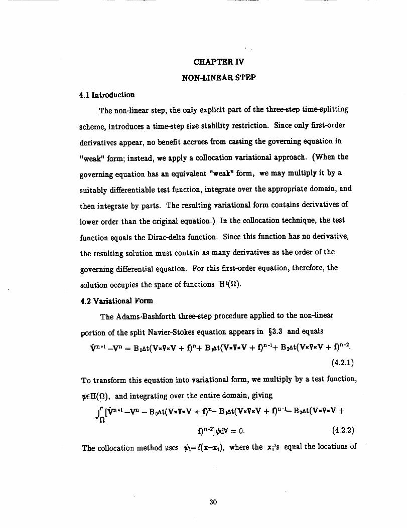
4.1 Introduction

The non-Linear step, the only explicit part of the three-step time-splitting

scheme, introduces a time-step size stability restriction. Since only first-order

derivatives appear, no benefit accrues from casting the governing equation in

"weak" form; instead, we apply a collocation variational approach. (When the

governing equation has an equivalent "weak" form, we may multiply it by a

suitably differentiable test function, integrate over the appropriate domain, and

then integrate by parts. The resulting variational form contains derivatives of

lower order than the original equation.) In the collocation technique, the test

function equals the Dirac-delta function. Since this function has no derivative,

the resulting solution must contain as many derivatives as the order of the

governing differential equation. For this first-order equation, therefore, the

solution occupies the space of functions Hl(fl).

4.2 Variational Form

The Adams-Bashforth three-step procedure applied to the non-linear

portion of the split Navier-Stokes equation appears in §3.3 and equals

_n.1 _V n = B_t(V=V=V + f)n+ BIat(V=V=V + t)n'l+ B_t(V=V=V + i')n-2.

(4.2.1)

To transform this equation into variational form, we multiply by a test function,

_H(_), and integrating over the entire domain, giving

r' [_Tn.l _V n _ BoAt(V=V=V + O n- BIAt(V=V=V + f)n-,_ B_At(V=V=V +Ja= 0.

The collocation method uses _i--_(I-Ii), where the xi's equal the locations of

3o

and

(The superscript e

into (4.3.1) gives

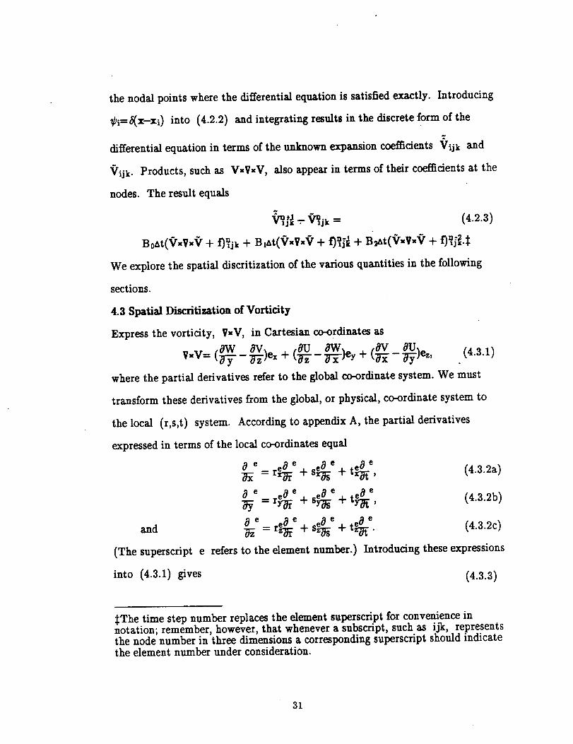
the nodal points where the differential equation is satisfied exactly. Introducing

_bi-6(x-xi) into (4.2.2) and integrating results in the discrete form of the

differential equation in terms of the unknown expansion coefficients Vijk and

Vijk- Products, such as V=VxV, also appear in terms of their coefficients at the

nodes. The result equals

V_l_ .-- _jk -_ (4.2.3)

We explore the spatial discritization of the various quantities in the following

sections.

4.3 Spatial Discritization of Vorticity

Express the vorticity, V=V, in Cartesian co-ordinates as

av (au _w av auwv= (_-y - _)e_ + _r- (_- _)e_,_--)ey + (4.3.1)

where the partial derivatives refer to the global co-ordinate system. We must

transform these derivatives from the global, or physical, co-ordinate system to

the local (r,s,t) system. According to appendix A, the partial derivatives

expressed in terms of the local co-ordinates equal

0 e -- r_ e S_ e t_ e, (4.3.2a,)+ +

o e ._ rez_e sez_e te_e (4.3.2C)+ + .

refers to the element number.) Introducing these expressions

(4.3.3)

:_The time step number replaces the element superscript for convenience innotation; remember, however, that whenever a subscript, such as ijk, represents

the node number in three dimensions a corresponding superscript should indicatethe element number under consideration.

31

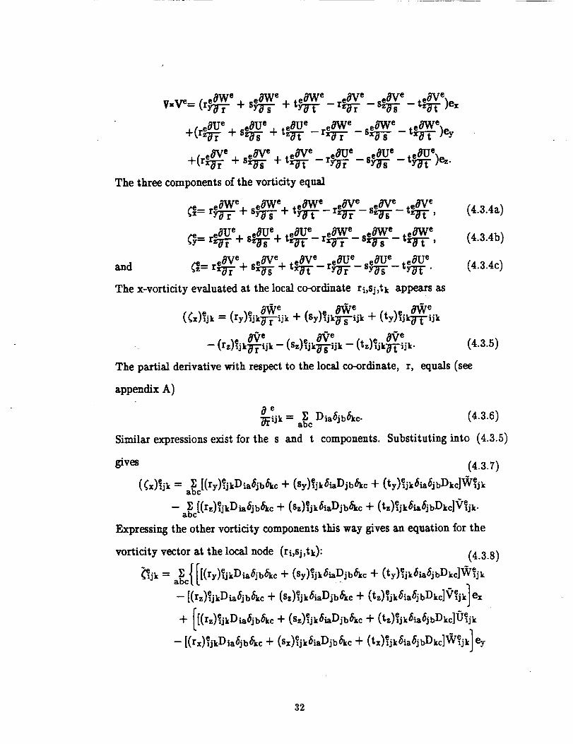
t-e _we __S e ,e 0Vv'e .eSVe _se ,eo"Vex..v-ve= _y-_-- + s + "Y_- - "_'d'_- - s - .z'_" j_x

, e0U e _eSU e .eSU e .eO_N e oeSV_ e_ t_t _e)eytr_-_- + o_ + _i- -_x_-_- -o_-

• .eSV • ,eSVe e _ _ t_t e)ez.+(r_- r + ox_- + ._--r_T r Se_Ue

The three components of the vorticity equal

_ex- r_--_-r e-_- S_-S e+ t_t e-- r_-r e- s_-/-- t_-t e,

_ey.= re_rU e_. se_s Ue.l. te_t Ue- r_-r e- s_-s e- t_-t e,

.e0Ve±.e0Ve±,eOVe eaU e seOUe +e_U eand _= _- _- Or-d_ -_ .r_-- rye-- _ -._-.

The x-vorticity evaluated at the local co-ordinate ri,sj,tk appears as

(_x)ejk = _ry),jk_-ijk _-

(rz)ej k__: :jk _ (sz)ejk__: iejk - ~e-- (tz)ejk_t ijk.

(4.3.4a)

(4.3.4b)

(4.3.4c)

(4.3.5)

The partial derivative with respect to the local co-ordinate, r, equals (see

appendix A)

_e----- Y_ Dia61b6kc._ijk abc

Similar expressions exist for the s and t components.

(4.3.6)

Substituting into (4.3.5)

gives (4.3.7)

(¢x)ejk = a_bc[(ry)ejkDia_jb_kc + (sy)ejk_iaDjb_kc + (ty)e_jk_ia_jbVkc]Wejk

e . -¢.

--a_bc[(rz)ejkDia_jb_kc + ($z)ejk_iaDjb_lkc -{- (tz)ljk_ia_jbDkc]V_jk.

Expressing the other vorticity components this way gives an equation for the

vorticity vector at the local node (ri,sj,tk): (4.3.8)

_jk--a_C{ [[(ry)_jkDia_jb_c-_-(S,)_jk_Djb_c "_" (ty)_jk_ia_jbDkc]*_jk

+ + + (t,) ,jk jbmkc]0 ,jk

32

r

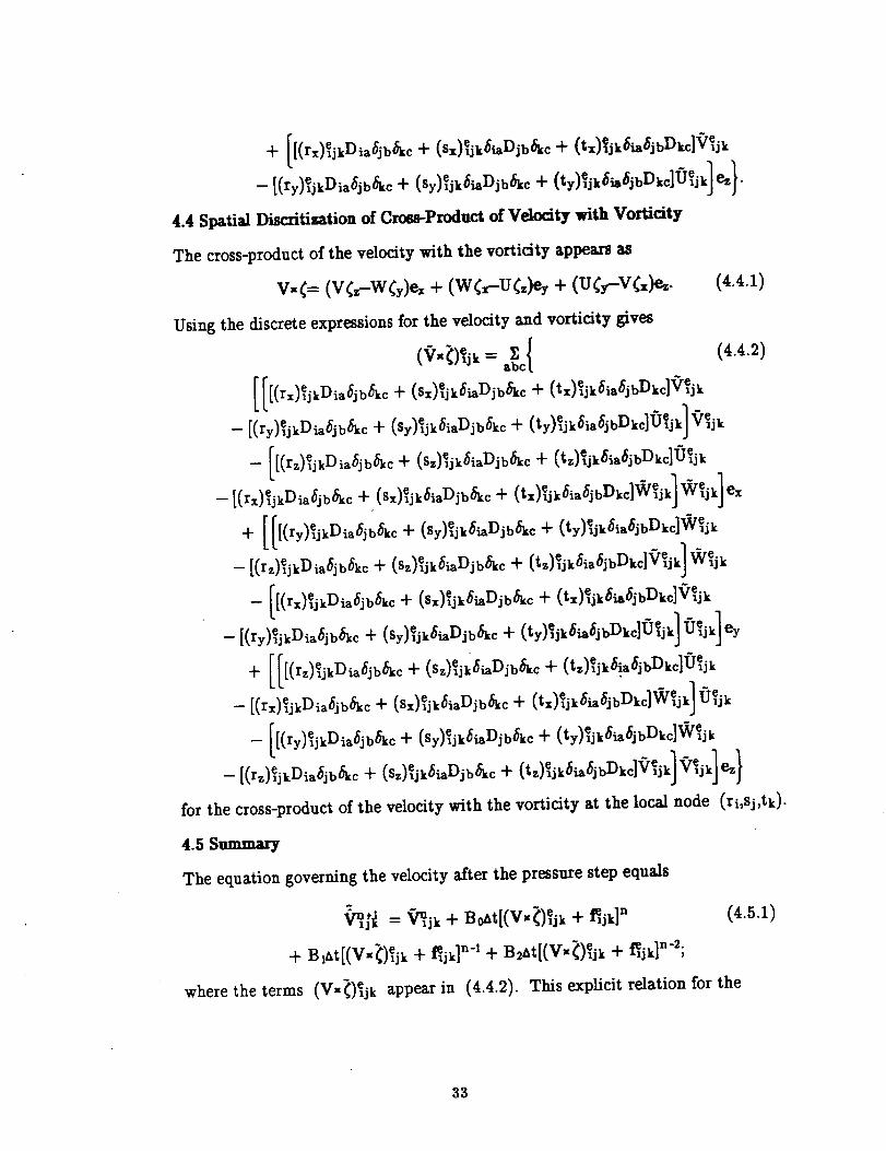
4- _[(rx)ejkDia6jb6kc 4- (sx)ejk6iaDjb6kc 4- (tx)ej k _ia_i bD kc]Vej k

--[(ry)_jkDia_jb_kc + ($y)eljk_iaDjb_kc + (ty)ejk_ia_jbDkc]UejkJez I.

4.4 Spatial Discritization of Cross-Product of Velocity with Vorticity

The cross-product of the velocity with the vorticity appears as

v.¢= (v&-wG)ez + (w&--u¢,)ey + (ucy--v&)e,. (4.4.1)

Using the discrete expressions for the velocity and vorticity gives

(V"_)_jk-- ...-_cl (4.4.2)

[[[(rx)ejkDia_jb_kc -{- (Sx),ejk_iaDjbOCkc + (tx)_jk_ia_jbDkc]'Qejk

- I(ry)Tj_D_jb_c + (sr)_6iaDjb_c + (ty)_j_Sia6jbDkc]Oe,i_]9_j_

t,. q..

J

- I[(r_)%kD_jba_+ (S,)%k6_Djb_,C+ (t,)%k_,%bDkc]0%kt.

--[(rx)e_jkDia_jb_kc 4- (Sx)_jk_iaDjb_kc + (tx)_jk_ia_jbDkc]Wejk[W%k[exJ J

P P

4- [[[(ry)ejkDia_jb_kc + (Sy)ejk_iaDjb_kc + (ty)ejk _ia_j bDkc]Wej k

--[(rz)ejkDia_jb_kc + (sz)ejk_iaDjb_kc + (tz)eljk_ia_jbDkc]Vejk]

- [[(rx)%kDi,%b&c+ (Sx)%k6_Djb&_+ (t,)%k6i_%bDk49%kt.

--[(ry)%kDia6jb6kc "4- (Sy)%k6iaDjb6kc 4-(ty)e_jk6ia6jbDkc]0ejk[ 0ejk[eyJ .J

-- [(rx)eljkDia6jb6kc + (Sx)eljk_iaDjb6_c + (tx)eljk_ia6jbDkc]We_jk I

-- [[(ry)_jkDia_jb_kc 4- (Sy)e_jk_iaDjb6kc 4- (ty)%k6ia6jbDkc]Wejk

--[(rz)C_jkeia_jb_c 4- (Sz)_jk_iaejb_kc 4- (tz)_jk6ia_jbDkc]V'jk l'_/e_jk] ez}

for the cross-product of the velocity with the vorticity at the local node (ri,sj,tk).

4.5 Summary

The equation governing the velocity after the pressure step equals

"2

V_ = _jk + B0at[(V,,_)%k + i_,jk]n (4.5.1)

+ Blat[(V*_)e, ik + _jk] n'l + B2At[(V"_)_jk + _jk]n'2;

where the terms (Vx_)_jk appear in (4.4.2). This explicit relation for the

33

unknownvelocity coefficientsat time step n+l dependson knownquantities

from the previousstep, denotedby the superscript n. Its solution doesnot

involve inverting the stiffnessmatrix; unfortunately, however, this simplicity

comes with a concomitant loss of accuracy-the collocation scheme searches for

the solution with a measurement device tolerating first-order errors in time.

34

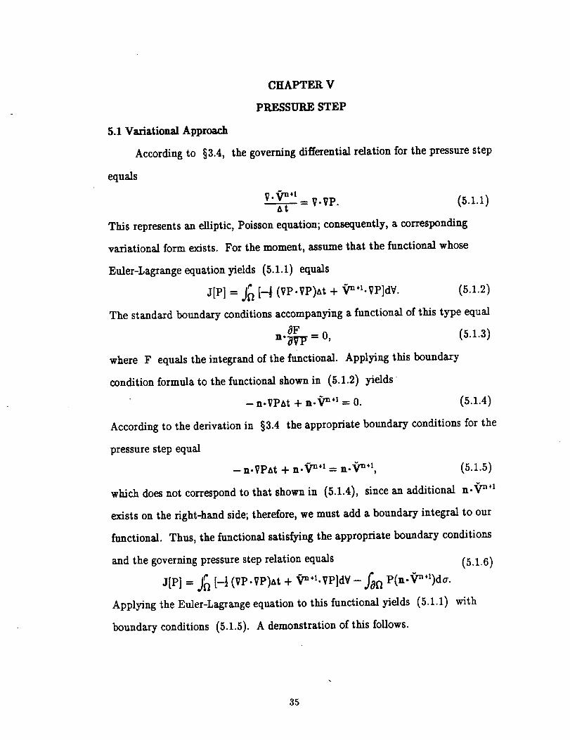
5.1 Variational Approach

According to §3.4,

equals

CHAPTER V

PRESSURE STEP

the governing differentialrelationfor the pressure step

V._ rnvl

A-----i--= V.PP. (5.1.1)

This representsan elliptic,Poisson equation; consequently, a corresponding

variationalform exists.For the moment, assume that the functionalwhose

Euler-Lagrange equation yields (5.1.1)equals

J[P] = J_ [--_ (VP-VP)_t + x_/n*"VP]d¥. (5.1.2)

The standard boundary conditions accompanying a functional of this type equal

n. p = 0, (5.1.a)

where F equals the integrand of the functional. Applying this boundary

condition formula to the functional shown in (5.1.2) yields

-n-VPAt + n-_ rn*l -- 0. (5.1.4)

According to the derivation in §3.4 the appropriate boundary conditions for the

pressure step equal

-n-VPat + n-_gn*1 = n-_/"n*1, (5.1.5)

which does not correspond to that shown in (5.1.4),since an additional n-_ rn'1

existson the right-hand side;therefore,we must add a boundary integralto our

functional. Thus, the functionalsatisfyingthe appropriate boundary conditions

and the governing pressure step relationequals (5.1.6)

J[P] = J_l [-_ (VP-VP)at + vn*1-VP]d¥ - f_f/P(n-_gn'*)da.

Applying the Euler-Lagrange equation to this functional yields (5.1.1) with

boundary conditions (5.1.5). A demonstration of this follows.

35

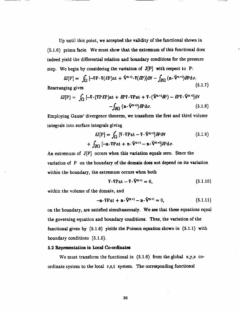
Up until this point, we accepted the validity of the functional shown in

(5.1.6) prima faeie. We must show that the extremum of this functional does

indeed yield the differential relation and boundary conditions for the pressure

step. We begin by considering the variation of J[P] with respect to P:

_[P]- J_ [-VP-V(o"P)At + (n-Qn+')o"Pdcr.

Rearranging gives (5.1.7)

(J[P]- j_ [-V.(VPo_P)At + oTV-VPAt + V-(_/_'t6P)- 5PV-Qn'I]dY

-fan (5.1.8)Employing Gauss' divergence theorem, we transform the first and third volume

integrals into surface integrals giving

_[P] = j_ [V-VPAt - V._rn*1]_Pd¥ (5.1.9)

+ fsfl [-n.VPAt + n._rn+l- n-'_v'n'll6Pd_.

An extremum of J[P] occurs when this variation equals zero. Since the

variation of P on the boundary of the domain does not depend on its variation

within the boundary, the extremum occurs when both

V-VPt_t - V._ ra'l = O, (5.1.10)

within the volume of the domain, and

-n.VPAt + n._ rn't - n-'_¢"n't = 0, (5.1.11)

on the boundary, are satisfied simultaneously. We see that these equations equal

the governing equation and boundary conditions. Thus, the variation of the

functional given by (5.1.6) yields the Poisson equation shown in (5.1.1) with

boundary conditions (5.1.5).

5.2 Representation in Local Co_rdinatm

We must transform the functional in (5.1.6) from the global x,y,z co-

ordinate system to the local r,s,t system. The corresponding functional

36

representation for a single element, designated by the superscript e, in local co-

ordinates equals

a[Pl'= f.'j'_',f.'[-I (vP.vP)_t+ V.vel'ldet[J'lId_dsdt

f 'f' P'(n-_)dA", (5.2.1)--p =l*_-I# -I

where we &op the superscriptindicatingthe time step number and replaceitby

a superscriptindicatingdement number. (Consult appendix B for detailsof the

volume dement conversion from globalto localco-ordinates.)The surface

integralcontains expressionsfor the summation over the six facesof each

dement. We willconsider the detailsof these terms later.

This functional,approximated by expressing itin terms of the expansion

polynomials, for example, Pe_cPebc_ba(r)Ibb(S)Ibc(t),__appears as

EP1e-"f_',.f.',j'_',6

+ Veabc •VibcP_bc]Iba(r)0b(S)Ibc(t)ldet[Je][abc&dsdt -- _ IPe.p=1

A briefexplanation of the accompanying notation seems appropriate. The

subscript abc refersto the node ra,Sb,tc,while the tilderefersto the

corresponding unknown expansion coefficients.We postpone treatment of the

0

surfaceintegral,conveniently expressed in the interim as P.Ipe, until §5.3.p--1

Many of the followingnumerical minutiae receivea more thorough

treatment in the followingchapter dealing with the viscous step. The gradient

operator in global co-ordinatesequals

In the local co-ordinate system this operator equals

e ~eVabcPabc --

_e _ebccse_ _e

(5.2.3)

(5.2.4)

37

8pebct_e_ "•[_r_)abc + _y)abc + _-y]aDcj_y +

~e

[_re)abc _e _t se)abc]es.+ _'(S_)abc +

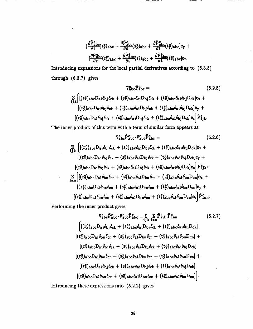
Introducing expansions for the local partial derivatives according to (6.3.5)

through (6.3.7) gives

re. _e. (5.2.5)_,DC aDC _-_

i_k[[(re)abcDai6bj6ck -t- (Sxe)abc_aiDbj6ck -t- (txe)abc6aiSbjD_]ex +

[(r_)abcDai_bj_ck -1- (S_)abc_aiDbj_ck "}" (t_)abc_ai_bjDck]ey "}-

e D -_ _e

The inner product of this term with a term of similar form appears as

e -e e "e (5.2.6)VabcPabc" VabcPabc ----

I[(rxe)abcDai6bj6ck -{- (Sxe)abc6aiDbj_ck -t- (txe)abc6ai6bjDck]ex -I-ijk L

[(r_)abcDai_bj6ck -t- (S_)abc6aiDbj_ck -F (t_)abc6ai_bjDck]ey -F

[(r_),bcD,_6bj6ck+ (se),bc_,iDbj6_k+ (te),bc6,i6bjDc_]e_]_jk"

l_n{[(rxe)abcDal_om6cn + (Sex)abc6alDbm6cn + (txe)abc_al6b-Dcn]ex +

P

[(r_)abcDal6bm6cn + (S_)abc6alDbm6cn -I- (t_)abc6al6bsDcn]ey q-

[(re)abcDal_bm_cn "F (se)abc_alDbm6cn -I- (te)abc6alSb,,Dcn]ezJ PTffin.

Performing the inner product gives

ve _e rTe _eabc abc'Vabc abc=i_k lsn_ _ejk P_-n (5.2.7)

[[(rxe)abcDai_bj_ck + (Sxe)abc_aiDbj_ck (te)abc_ai_bjDck]+

[(re)abcDal6bm6cn + (Sxe)abc6alDbm_cn + (txe)abc_al_bmDcn]-t-

[(r_)abcDai_bj_ck -1- (S_)abc_aiDbj_ck + (t_)abc_ai_bjDck]

[(r_)abcDal_bm/_cn + (S_)abc_alDbm_cn -t- (t_)abc_al_o-Vcn] -i-

[(rze)abcDai_bj_ck -F (sez)abc_aiDbj_ck _- (tze)abc_ai_bjDck]

[(rze)abcDal_bmEcn -t- (Sze)abc_,lDbffi_cn -F (te)abc_al_bsDcn]l.

Introducing these expressions into (5.2.2) gives

38

[(rxe)abcDai6bj6ck -t- (Sxe)abc6aiDbj6ck + (txe)abc6ai6bjI)ck]

[(rxe)abcDal6bm_cn _- (sxe)abc6alDbu6cn -I- (txe)abc6alSbuDcn] "{-

[(r_)abcDal6bm6cn ÷ (S_)abcSalDb-6cn + (t_)abc6al6bmVcn] +

[(re)abcDa16bu6cn + (se)abc6alDbm6¢_ -I- (tez)abc6al6bmDcn]lJ

-I- _rebc'i_kI[(re)abcDai_bj_ck Jr (se)abc_aiDbj_ck -}- (te)sbc_ai_bjDck]ex _-

[(r_)sbcDai_bj_ck Jr ($_)sbc_aiDbj_ck _- (t_)abc_ai_bjDck]ey -_

[(rze)abcDai_bj_ck + (8ze)abc_aiDbj_ck + (tze)abc_ai_bjDck]ez] lSejk ] drdsdt

6- _.Ip_. (5.2.s)

p=I

Evaluating the integrals by introducing wa--f__'¢.(r)dr according to (1.5.16)

gives

j[p]e=__ Z Z _ Pe_jkP_unAtWawbWc]det[Je]lab cabc ij k lun

[(rxe)abcDai_bj_ck _- (se)abc_aiDbj_ck + (txe)abc_ai_bjDck]

[(rxe)abcDal6bm_cn "}- (sxe)abc_alDbm$cn _- (txe)abc_aI_buDcn] -i-

[(r_.),b_D,_j_ck+ (S_.)abJ,_Dbj_c_+ (t_,),b¢_,_bjDck]

[(r_)abcDal_m_cn + (S_)abc_alDbu_cn "}" (t_)abc_al_buDcn]-{-

[(re)_.b_D,_¢k + (St),b_Dbj_c_+ (tt)_,bJ,,_bjDc_]

[(rze)abcDal_b._cn Jr (Sze)abc_alDb.$cn "t- (tze)abc$al_b.Dcn]]

"1" ab_c Vebc" ij_k Pe_jkWsWbWcl det[Je] [ abc

[(re)abcDai_bj_ck -{- (se)abc_aiDbj$ck -{- (tex)abc_ai_bjDck]ex -{-

[(r_)abcDai_bj_ck -i- (S_)abc_aiDbj_ck + (t_)abc_ai_bjDck]ey 4-

($ze)abc_aiDbj_ck -t- (te)abc_ai_bjDck]ez][(r_),_cDa_aj_¢_+

- _;_. (5.2._)p=!

39

Excluding the surface integral, this represents the governing functional in terms

of the local co-ordinates.

S.3SurfaceIntegral

The surface integral,

contains contributions from each of the six sides of each element.

(s3.1)

We must

express it in terms of the unknown expansion coefficients in the local (r,s,t) co-

ordinate system. Rearranging (5.3.1) by combining the surface unit normal

vector, n, with the differential area, dA, gives

' _ f Ifi (5.3.2)iPe _ pete. dAP.p'l p=l *1-1 "l-1

Introducing these expressions for each of the six faces on the local dement gives

6I pe -- (5.3.3)

p=!

-f.,f_'peve-(x,ex + ysey + z3ez)drds

+_" I_'I pe_.(x_e x + y2ey + z2ez)drdt-1 '¢ -1

+( ,(I pe_e.(x3e x + y3ey + z_ez)drds_' -1 ,s -1

--/-'1/-: peve'(x_ex + y2ey + z_ez)drdt

_f. ;f.11 pe_. (xlex + yley +z le_)dsdt

+( 1_'1 pe,_/e.(xlex + yley + zlez)dsdt,-1 ,/-1

where we expressed the area vectors shown in (5.3.2) in terms of their

component parts with the assistance of §A.7 in appendix A. Introducing the

expansion polynomials into these surface integrals gives

6zIpe=

pffil

-f_,f, PebiVeb1-(x,ex + y,ey -{-z,ez)ab,_a(r)_(s)drds

-l-/"'(" Z pae,cVe2c.(X2ex+ y2ey -I-z:e.z)a2cCa(r)_bc(t)drdt-I,s-I ac

(5.3.4)

4O

+f 'l"*/-I_"-I

I I bc

+f'f'-I,_-I bc

_ Peb_'[e_.(_3e.+ y_y+ -_)_,2_(r)_b(s)d_ds

P_a,c_,c"(_ + Y_y+ _)_,c¢_(_)¢_(t)d_dt

P_bcV_bc" (xlex + y tey -{- zlez) ibc_o($)_dt)clsdt

P_bc_bc'(xlex + yley + zlez)2bc_b(S)_dt)dsdt.

Evaluating the integrals using wa-/'l_/A(r)clr gives

6EIpe

pffi!

--a_b PeblVebl.(x3ex -I- y3ey -I" z3ez)ablWaWb

_e _re .tX^+ _ a2cVa2c t _x + y_ey + Z_.z)a2cWaWcac

+a_b Peb2Veb2" (X3ex + y3ey + z3ez)ab2WaWb

- I__ae_cV_ic•(x_ex+ y_ey+ z_e_)ajcWaWcac

--bc_ P_bcV_bc • (xlex -I- yley + zlez)ibcWbWc

(5.3.5)

+bc_ P_bcV_bc" (xlex + yley + zlez)2bcWbWc.

e e V e W e givesFinally, performing the inner product using Vabc--Uabcex+ abcey+ abce, z

6

Ipe _ (5.3.6)p=l

-- _ pebl(UeblX 3 -[- Veably3 + WeblZ3)ablWaWbab

_3e /U e X Wea2cZ2)a2cWaWcJr _ xa2ct a2c 2 "t" Ve2cY2 Jrac

+ab _ 15aeb2(Uaeb2X 3 + Veb2y_ -b Web2z_)ab2WaWb

- S P_c(U_cX2 + V_cy2 + W_cZ2)a_cWaWcac

-- _ P_bc(U_bcXl + V_bcYl + W_bcZl)IbcWbWcbc

P_bc(U_bcXl + V_bcYl + W_bcZl)2bcWbWc -+be

41

5.4 Variation of the Pauctional

All of the pieces corresponding to the terms in the governing functional

exist in terms of the local co-ordinates and expansion functions and coefficients.

Substituting (5.3.6) into (5.2.9) and performing the remaining inner product

gives

j[p]e = .._ Z Z _nPe_jk P_nbtWawbWc[ det[Je]lsbcabc ij k

[(re)abcDai_bj_ck -t- (Sxe)abc_aiDbj_ck + (txe)abc_ai_ojDck]

[(re)abcDal6bm6cn % (se)abc6alDbm6cn -F (txe)abc6al6bmDcn] %

[(r_)abcDai6bj_ck + (S_)abc6aiDbj6ck + (t_)abc6ai6bjDck]

[(r_)abCDal_b._+ (S_),b_6,_Db.6_.+ (t_)_b_,]Z_.Dc,]+e

[(rez)abcDai_bj6ck "t- (sze)abc6aiVbj6ck -t- (tz)abc6ai_bjDck]

[(r_),bcD_6b.6c_+ (se),b_Db.6_ + (te),b_6,_6b.D_]1

+ _ _ pejkWaWbWc[det[Je]labcabc ij k

[(rxe)abcDai_bj_ck + (Sxe)sbc_aiDbj_ck + (te)abc_ai_bjDck]_ebc_ -

[(r_)abcDai_oj_ck _" (S_)abc_aiDbj_ck Jr (t_)abc_ai_bjDck]Vebc_ -

e Dck]_ve]

- _ _eb,(Ueb_x3+ VXb_s+ W_b_Zs)_b_WaWbab

+ r. _e_(ue_cx_+ V%cy_+ we_cz_)a_cwawc

_eb_(fl_b_X_+ Qeb_yS+ Web_.S),b_W_Wb4"ab

_ y._e_(ue,cx_ + ve_cy_+ Vv'et_z2)stcW_Wc

The extremum of J[P],

ac

-- ]] P_bc(U_bcX1 "4"V_bcYl "]- W_bcZl)IbcWbWcbc

P_bc(U_bcXl "I-V_bcYl + W_bc_l)2bcWbWc.+bc

or the variation OJ[P]/OP, equals

42

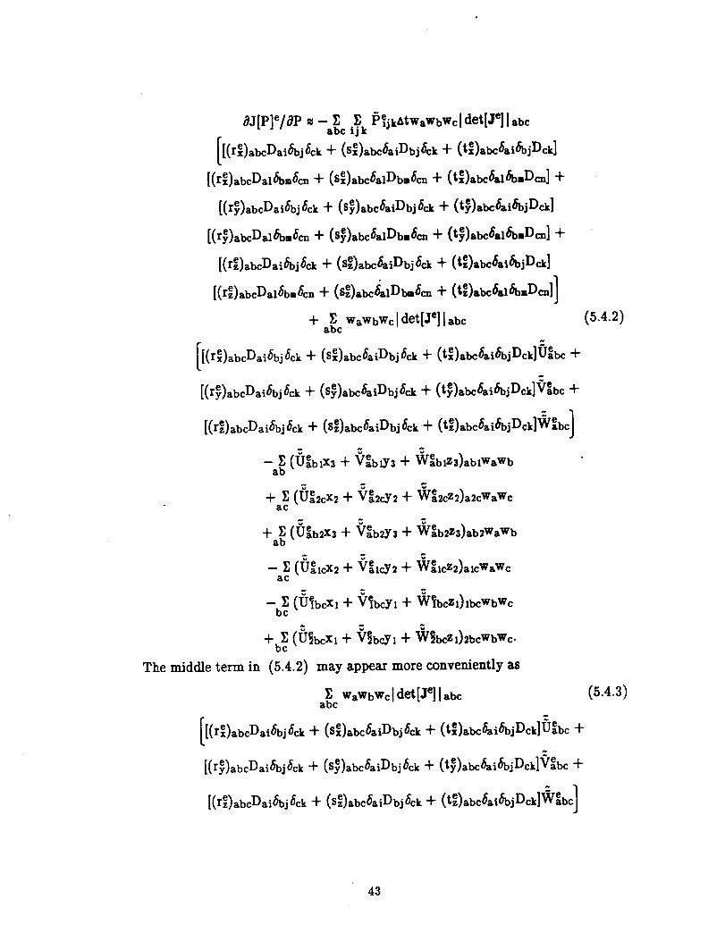
8j[p]e/_p __ y_ y, _ejkAtwaWbWc[det[Je]lab cabc ij k

[(rxe)abcDai6bj_ck 4- (Sxe)abc6aiI)bj_ck + (txe)abc6ai6bjDck]

[(re)abcDal6bu6cn + (sxe)abc_alDbu6cn + (txe)abc6al4_buDcn] +

[(r_),bcD,_6bj6_k+ (S_)abc_,_Dbj6ck+ (t_),b_,_6bjD_k]

[(r_),b_D,_6b.6_+ (S_),bc6,_Db._ + (t_),b_,,6b.D=] +

re D • "_[( z),bc ,,6bj ck+ (S'_),b_iDbj6ck+ (t',),b_6,t6bjD_k]

re D _, (se)abc_alDbm6cn q" (tze)abc6aldSbuDcn]J[( ,.),bc_6b. _. +

q- _ WaWbWcldet[Je]labcabc

[(re)abcDai_bj_ck -_ (se)abc_aiDbj6ck _- (tex)abc_ai_bjDck]0eabc +

[(r_)abcDai_bj_ck _r (S_)abc_aiDbj_ck _" (t_)abc_ai_biDck]Vebc +

e D _v'e 1[(re)abcDai_bj6ck -}- (sez)abc_aiDbj_ck+ (tz)abc_ai_bj ck] abcJ

-- E (UeblX._ + VeblY3 -[- V_eblz3)ablWaWbab

_- _ (We2cx2 + Ve2cY2 _- wea2cZ2)a2cWaWcac

"}-ab_ (Ueb_x3 + Veb_y_ _- Web2z3)ab2WaWb

- _,(Uezcx2+ V_Icy2+ Welcz_)alcW,Wc&c

-- _ (U_bcXl "4-V_bcYl "}-W_bcZl)IbcWbWcbc

_-bc_ (_bcXl + _bcYl "}"_]bcgl)2bcWbWc"

The middle term in (5.4.2) may appear more conveniently as

S WaWbWc[ det[Je] Iabcabc

[ -[(rex)abcDai_bjhk_- (se)abc_aiDbj_ckuc (txe)abc_ai_bjDck]Uebc-_

[(r_)abcDai_bj_ck-F (S_)abc_aiDbj_ck+ (t_)abc_ai_bjDck]Vebc"{"

e D _V e

(5.4.2)

(5.4.3)

43

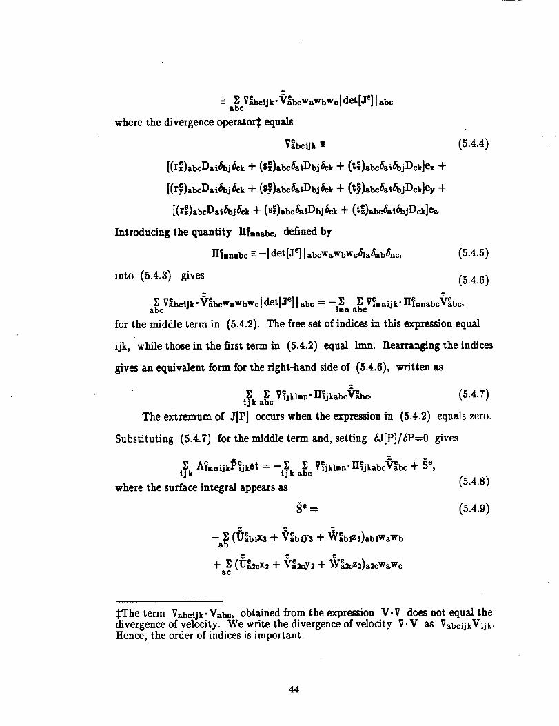
= a_bcVebcijk-_ebcWaWbWc[ det[Je] [ abe

where the divergence operator:[: equals

Vebeijk --

[(rxe)abcDai6bj6ck -I- (sxe)abc6aiDbj6ck "I- (txe)abc6ai6bjDck]ex +

[(r_)abcDai_bj_ck -I- (S_)abc_aiDbj_ck "I- (t_)abc_ai_bjDck]ey +

[(re)abcDai6bj6ck + (sze)sbc_aiDbj6ck -I" (tze)sbc6ai6bjDck]ez.

Introducing the quantity IITanabc, defined by

HT-nabc - -[det [Je] [ abcWaWbWc_la_b_nc ,

into

(5.4.4)

(5.4.5)

(5.4.3) gives (5.4.6)

ab_cVebcijk "VebcWaWbWc I det[Je] I abc -" --l_n ab_c VTunijk" H_mnabcVeabc_

for the middle term in (5.4.2). The free set of indices in this expression equal

ijk, while those in the first term in (5.4.2) equal hnn. Rearranging the indices

gives an equivalent form for the fight-hand side of (5.4.6), written as

The extremum of

_ Ve_jklmn" H e'ljj_aoc" V e'aDc- (5.4.7)ij k abc

J[P] occurs when the expression in (5.4.2) equals zero.

Substituting (5.4.?) for the middle term and, setting _J[P]/EP=0 gives

A_mnijk_ejkAt =_ _ _ Vejklmn.iie... _e.ijk ijk abc 1JKaoc aoc "}" _e,

where the surface integral appears as

-- _" (UeablX3 -I- VaeblY3 + Weblz3)ablWaWbab

_ v v

+ I1 (l/_cX_ + V_2 + W_2eZ_)a2eWaWcac

SThe term Vabcijk'Vabc, obtained from the expression V.V does not equal thedivergence of velocity. We write the divergence of velocity V. V as VabcijkVijk.

Hence, the order of indices is important.

44

(Ueb2x3 _- Veb2y3 -i-Web_zl)ab_WaWb"l'ab

- II (U_l_ + V_l_7_ + W_lcZ_)alcWaWeac

-b_ (U_bcX_+ VTbcY_+ W_z_)zbcWbW_• _, v v

_'bc_ (U_bcXl + V_bcYl 4" W_bcZl)2bcWbWc,

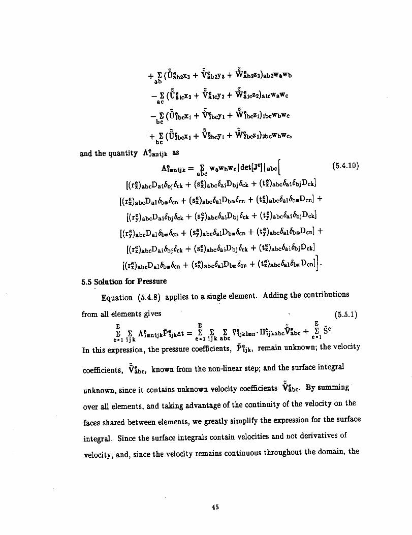
and the quantity A_mnijk as

A_mnijk = a_bcWaWbWc]det[Je] [abc[

[(r_)abJ)ai6bj6c_+ (S_)abc6_iI)bj_ok+ (t_),b_6bjD_k]

[(r_)ab¢I)_16b,6c_+ (S_)_bc6_lDb,6_n+ (t_)ab¢6_6b,Dc_]+

[(r_)abcI)ai_bj_ck-{-(S_)abc_aiI)bj_ck + (t_)abc_ai_bjDck]

[(r_)abcDal_bu6cn + (S_)abc6alDbm6cn + (t_)abc_al6b.Scn] +

[(rze)abcDaiSbj/_ck+ (se)abc_ail)bj_ck+ (te)abc_ai_bjSck]

[(ze)abcDal_bm6cn -I-(se)abc_alDbm_cn -F (te)abc_al_bmDcn]].

5.5SolutionforPressure

(s.4._0)

Equation (5.4.8)appliesto a singleelement. Adding the contributions

from all elements gives (5.5.1)

E E = E

Z Z A_mniikl_ejkAt = Z Z S Vejklmn. IIe'" " V e"e-*l ijk ell ijk abc _a_c at)c % e=l_" _e.

In this expression, the pressure coefficients, P_jk, remain unknown; the velocity

coefficients, Veabc, known from the non-linearstep;and the surfaceintegral

unknown, sinceitcontainsunknown velocitycoefficientsVaebc. By summing

over all elements, and taking advantage of the continuity of the velocity on the

faces shared between elements, we greatly simplify the expression for the surface

integral. Since the surface integrals contain velocities and not derivatives of

velocity,and, sincethe velocityremainscontinuousthroughoutthe domain, the

45

terms cancel on faces shared between two elements. Thus the summation over all

elements yields a contribution from only those dements on the boundary of the

domain. Unfortunately, the surface integral contains unknowns which represent

the velocity after the pressure step. Hence, (5.5.1) contains two unknowns:

v

pressure Pe_jk and velocity V_jk. Along surfaces where we specify essential

boundary conditions on velocity, the surface integral depends on known

quantities; along surfaces where we specify natural boundary conditions, the

velocity, V_jk, remains unknown. We may circumvent this problem by

approximating the surface integral of n'V along natural boundaries by n-_',

since we know V from the non, near step. However, since V does not satisfy

boundary conditions, a significant error may accrue from these integrals;

furthermore, these integrals over the boundaries where both natural and essential

conditions occur may require extensive computational time. Therefore, we use an

entirely different technique for the surface integral expression.

E

Since _. _e represents the net flux of velocity leaving the domain,e--1

ff_(n-V)dA, we choose to compute the integral of n-_" over the inlet and

exit boundaries and apply the difference of these terms to the exit velocity in the

form of a correction. Hence, no longer do we satisfy (5.5.1) exactly at each of

the nodal points. Instead, (5.5.1) holds only in a "global" sense. We

approximate the surface integral by

E

_e _ Vout'_oute=!

-- fSainn-_'d, +/_/_outn-_'da, (5.5.2)

where Pout equals the average outflow velocity correction and Aout equals the

outflow area. The velocity correction applies to the velocity after the non-linear

46

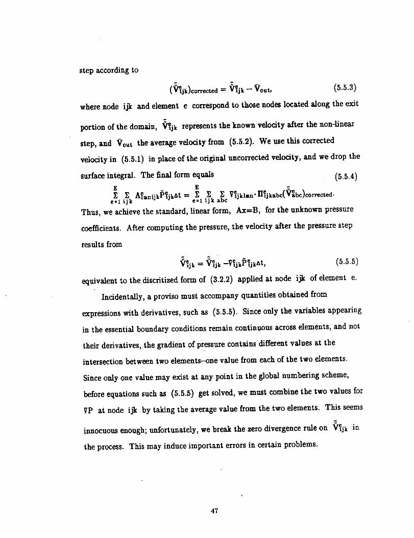
step according to

(5.5.3)

where node ijk and element e correspond to those nodes located along the exit

portion of the domain, V_jk represents the known velocity after the non-linear

step, and Vout the average velocity from (5.5.2). We use this corrected

velocity in (5.5.1) in place of the original uncorrected velocity, and we drop the

su_rface integral. The final form equals (5.5.4)E E ~

I; AT=nijkP_jkAt = l; l_ I; VC,jkl=n. II_jkabc(_re_bc)co_cted.e=! ijk e=l ijk abc

Thus, we achieve the standard, linear form, Ax=B, for the unknown pressure

coefficients. After computing the pressure, the velocity after the pressure step

results from

V_jk Vejk e. "e. (5.5.5)-- -VijkP ljkAt,

equivalent to the discritized form of (3.2.2) applied at node ijk of element e.

Incidentally, a proviso must accompany quantities obtained from

expressions with derivatives, such as (5.5.5). Since only the variables appearing

in the essential boundary conditions remain continuous across elements, and not

their derivatives, the gradient of pressure contains different values at the

intersection between two elements-one value from each of the two elements.

Since only one value may exist at any point in the global numbering scheme,

before equations such as (5.5.5) get solved, we must combine the two values for

VP at node ijk by taking the average value from the two elements. This seems

innocuous enough; unfortunately, we break the zero divergence rule on V_jk in

the process. This may induce important errors in certain problems.

47

CHAPTER VI

VISCOUS STEP

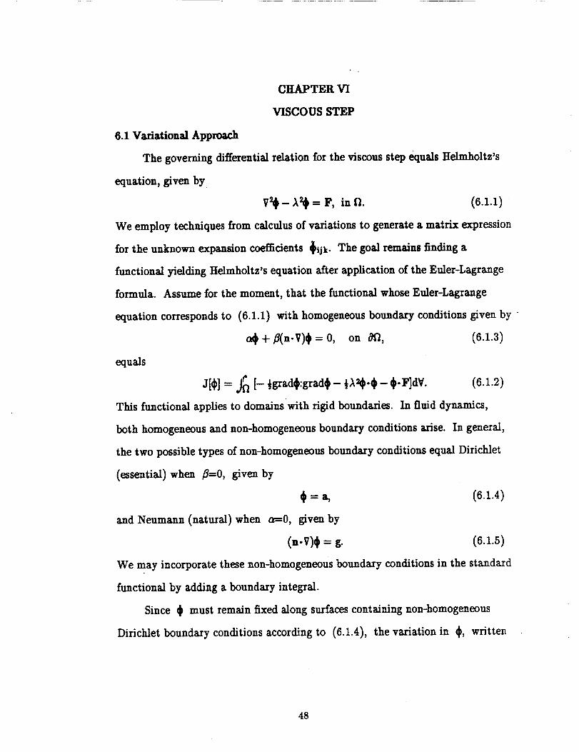
6.1 Variational Approach

The governing differential relation for the viscous step equals Helmholtz's

equation, given by

V_- A_ = F, in fL (6.1.1)

We employ techniques from calculus of variations to generate a matrix expression

for the unknown expansion coefficients _ijk. The goal remains finding a

functional yielding Helmholtz's equation after application of the Euler-Lagrange

formula. Assume for the moment, that the functional whose Euler-Lagrange

equation corresponds to (6.1.1) with homogeneous boundary conditions given by "

o4+ _(,,.v)_= o, on _, (6.1.3)

equals

J[_)]= j_ [- ½grad_:grad_ - ½A_-_- _-F]d¥. (6.1.2)

This functional appliesto domains with rigidboundaries. In fluiddynamics,

both homogeneous and non-homogeneous boundary conditionsarise.In general,

the two possibletypes of non-homogeneous boundary conditionsequal Dirichlet

(essential)when /_-0, given by

_=a,

a----O, given by

(n-v)_= g.

and Neumann (natural) when

(6.1.4)

(6.1.s)

We may incorporate these non-homogeneous boundary conditionsin the standard

functionalby adding a boundary integral.

Since @ must remain fixedalong surfacescontaining non-homogeneous

Dirichletboundary conditions according to (6.1.4),the variationin _, written

48

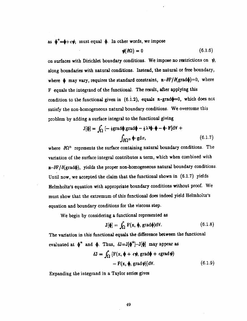
as (_*-----_+ e_b, must equal _. In other words, we impose

(on) = 0 (6.1.6)

on surfaces with Dirichlet boundary conditions. We impose no restrictions on _b,

along boundaries with natural conditions. Instead, the natural or free boundary,

where _ may vary, requires the standard constraint, n-_F/8(grad(_)=0, where

F equals the integrand of the functional. The result, after applying this

condition to the functional given in (6.i.2), equals n.grad(_=0, which does not

satisfy the non-homogeneous natural boundary conditions. We overcome this

problem by adding a surface integral to the functional giving

J[¢] = j_l [- ½grad(_:grad_- ½_.¢- ¢.F]dV +

fsan _.gda , (6.1.7)

where 8ft n represents the surface containing natural boundary conditions. The

variation of the surface integral contributes a term, which when combined with

n-aF/a(grad_), yields the proper non-homogeneous natural boundary conditions.

Until now, we accepted the claim that the functional shown in (6.1.7) yields

Helmholtz's equation with appropriate boundary conditions without proof. We

must show that the extremum of this functional does indeed yield Helmholtz's

equation and boundary conditions for the viscous step.

We begin by considering a functional represented as

J[_] = J_ F(x, _, grad(_)dV. (6.1.8)

The variation in this functional equals the difference between the functional

evaluated at _* and _. Thus, _=J[_*]-J[_] may appear as

&] = J_ IF(x, _ + elb, grad_ + egrad¢

- F(x, ¢, gradlb)]d¥. (6.1.9)

Expanding the integrand in a Taylor series gives

49

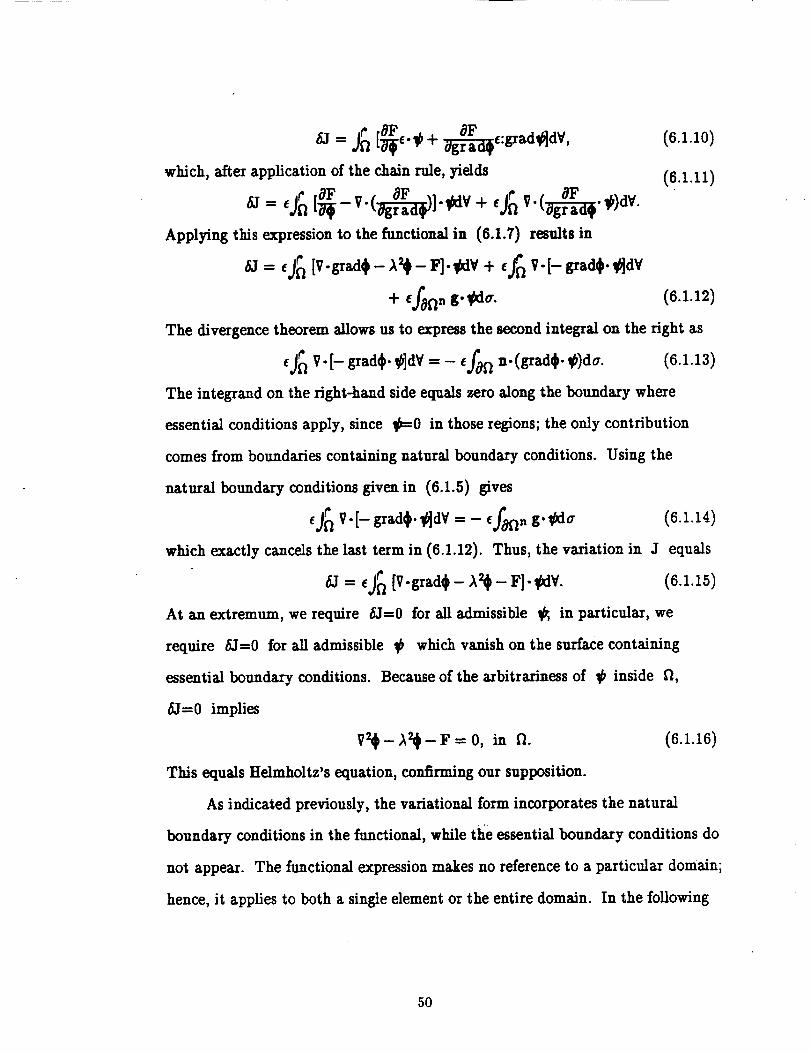
which, after application of the chain rule, yields

Applying this expression to the functional in (6.1.7) results in

- eJ_ [V-grsd_-A_-F]-lkl¥ + ej_ V-[-grad_. @]dV

+ efsf_n g-#de.

(B.i.lO)

(6.1.11)

(6.1.12)

The divergence theorem allows us to express the second integral on the right as

eJ_ V-[- grad_l._d¥ = - ef#fl n-(grad_l._)da. (6.1.13)

The integrand on the right-hand sideequals zero along the boundary where

essentialconditions apply, since _=0 in those regions;the only contribution

Using thecomes from boundaries containing natural boundary conditions.

natural boundary conditions given in (6.1.5) gives

eJ_ P-[--gradl_-_dV = - e/_n g-11_da (6.1.14)

which exactly cancelsthe lastterm in (6.1.12).Thus, the variationin J equais

= eJ_l [V-gradl_- A_I- F]-CdV. (6.1.15)

At am extremum, we require 5=0 for alladmissible _ in particular,we

require 6J=0 for alladmissible @ which vanish on the surfacecontaining

essentialboundary conditions. Because of the arbitrarinessof _ inside n,

6J=0 implies

V'_- A_- F = O, in fl. (6.1.16)

This equals IIelmholtz'sequation,confirming our supposition.

As indicated previously,the variationalform incorporates the natural

boundary conditionsin the functional,while ti_eessentialboundary conditions do

not appear. The functionalexpression makes no referenceto a particulardomain;

hence, itappliesto both a singleelement or the entiredomain. In the following

50

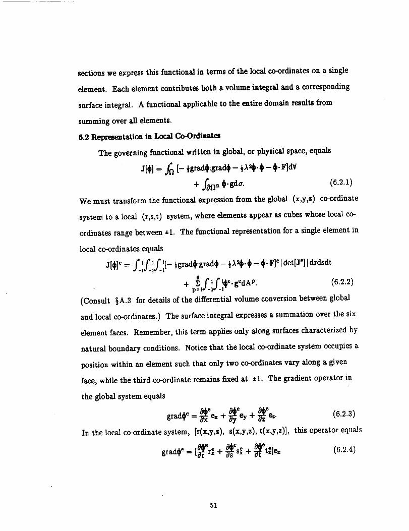
sections we express this functional in terms of the local coordinates on a single

dement. Each dement contributes both a volume integral and a corresponding

surface integral. A functional applicable to the entire domain results from

summing over all elements.

6.2 P,_resentafion in Local Co-Ordinates

The governing functional written in global, or physical space, equals

J[¢]= j_ [-,_ad_:_ad_- _._- #.Flay

+ f_° _.gd,. (8.z_)We must transform the functional expression from the global (x,y,z) coordinate

system to a local (r,s,t) system, where dements appear as cubes whose local co-

ordinates range between _1. The functional representation for a single element in

local coordinates equals

1 1 l_½grad_:grad_ ½A_.___.F]eldet[je][drdsdtJi'_le=f-I-l/.,[8

+ E (1(._e.gedAP" (6.2.2)p=1*I -lw -I

(Consult §A.3 for details of the differential volume conversion between global

and local co-ordinates.) The surface integral expresses a summation over the six

dement faces. Remember, this term applies only along surfaces characterized by

natural boundary conditions. Notice that the local coordinate system occupies a

position within an dement such that only two coordinates vary along a given

face, while the third coordinate remains fixed at _1. The gradient operator in

grad_e = _eex + _eey + _zeez.

the global system equals

In the local coordinate system, [r(x,y,z), s(x,y,z), t(x,y,z)],

(8.2.z)

this operator equals

(6.2.4)

51

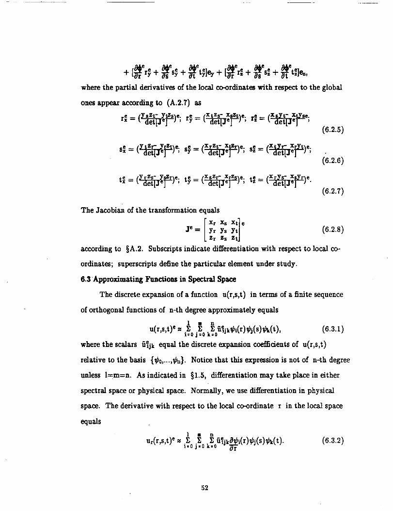
e e+tg,_+#,',_,+_,t,.l,.,,+t#',:+#,',:+_,°,:1_,where the partial derivatives of the local co-ordinates with respect to the global

ones appear according to (A.2.7) as

The Jacobian of the transformation equals

je= Yr Ys Yt (6.2.8)Zr Zs Zt

according to §A.2. Subscripts indicate differentiation with respect to local co-

ordinates; superscripts define the particular dement under study.

6.3Approximating Functions in Spectral Space

The discrete expansion of a function u(r,s,t) in terms of a finite sequence

of orthogonal functions of n-th degree approximately equals

1 m n

u(r,s,t) e _ _ _ k_oSejk_i(r)_j(S)_,(t), (6.3.1)i=0 j=0

where the scalars uejk equal the discrete expansion coefficients of u(r,s,t)

relative to the basis {tbo,...,1L'n}.

unless l=m=n. As indicated in

spectral space or physical space.

Notice that this expression is not of n-th degree

§1.5, differentiation may take place in either

Normally, we use differentiation in physical

The derivative with respect to the local co-ordinate r in the local spacespace.

equals

] [] n

Ur(r's't)e _ i=Oj=Ok_ _ _0uejk_r i(r)_j(s)_'(t)"

52

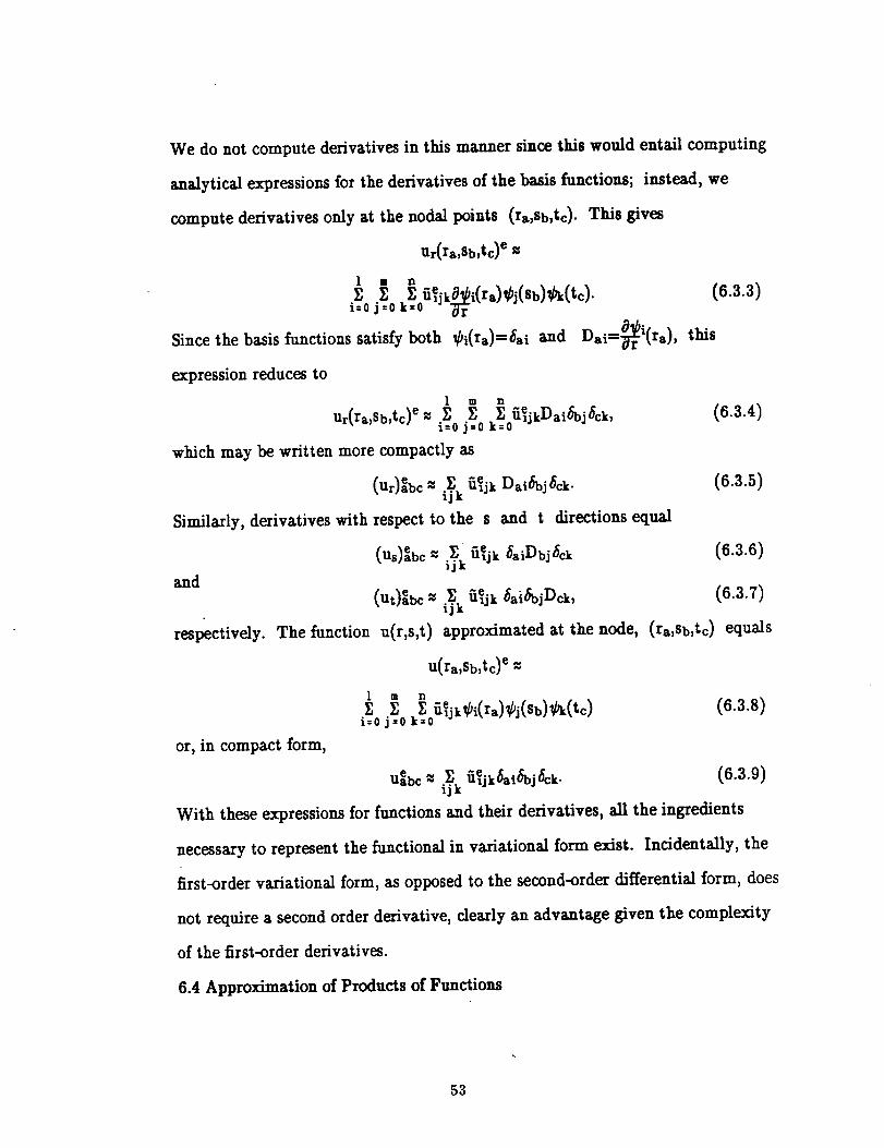
We do not computederivativesin this manner since this would entail computing

analytical expressions for the derivatives of the basis functions; instead, we

compute derivatives only at the nodal points (rs,sb,tc). This gives

Ur(ra,Sb,tc) e

| m n

_, _0U_j k_i(ra) _j($b) _k(tc).i--0 j =0 k

Since the basis functions satisfy both _i(ra)=Sai and

expression reduces to

(6.3.3)

Dai= i(ra), this

] m n

Ur(ra,sb,tc) e _ _ _ _ ueljkDai_bj_ck,iffi0 jffi0 kffi0

which may be written more compactly as

(ur)ebc "_ i_k 5e_jk DaiSbj_ck.

Similarly, derivatives with respect to the s and t directions equal

and

(us)ebc _ _ U_jk _aiDbj_ckijk

respectively.

(Ut)aebc = i{k 5e_jk _ai_bjDc_,

The function u(r,s,t) approximated at the node, (ra,Sb,tc)

u(ra,sb,tc)e

or,in compact form,

(6.3.4)

(6.3.5)

(6.3.6)

(6.3.:)

equals

1 m n

_, _, _=05ejk_bi(ra)_bj(Sb)_(tc) (6.3.8)i=0 j=0 k

uebc _ _ _ezjk_ai_oj_ck. (6.3.9)ijk

With these expressions for functions and their derivatives, all the ingredients

necessary to represent the functional in variational form exist. Incidentally, the

first-order variational form, as opposed to the second-order differential form, does

not require a second order derivative, clearly an advantage given the complexity

of the first-order derivatives.

6.4 Approximation of Products of Functions

53

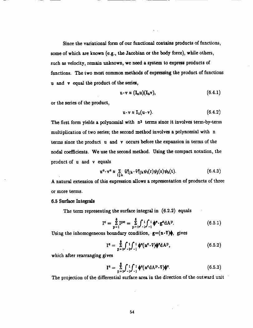
Sincethe variational form of our functional contains products of functions,

some of which are known (e.g., the Jacobian or the body force), while others,

such as velocity, remain unknown, we need a system to express products of

functions. The two most common methods of expressing the product of functions

u and v equal the product of the series,

u. v _ (Inu)(Inv), (6.4.1)

or the series of the product,

u-v = In(u'v). (6.4.2)

The first form yields a polynomial with n2 terms since it involves term-by-term

multiplication of two series; the second method involves a polynomial with n

terms since the product u and v occurs before the expansion in terms of the

nodal coefficients. We use the second method. Using the compact notation, the

product of u and v equals

ue've _ i_k _jk'Vejk_i(r)_J(S)_bk(t)" (6.4.3)

A natural extension of this expression allows a representation of products of three

or more terms.

6.6 Sudsce Integrals

The term representing the surface integral in (6.2.2) equals

I e - _ I pe = _}e._edAP. (6.5.1)p--1 pffil#-l_ -I

Using the inhomogeneous boundary condition, g=(n-V)_, gives

i e = _ f 1/'I _e(ne.V)_edAP ' (6.5.23p=l*r -1_ -I

which after rearranging gives

I e = _ {'1/'l_e(nedAP-V)_ e. (6.5.3)p=lW -1_ -1

The projection of the differential surface area in the direction of the outward unit

54

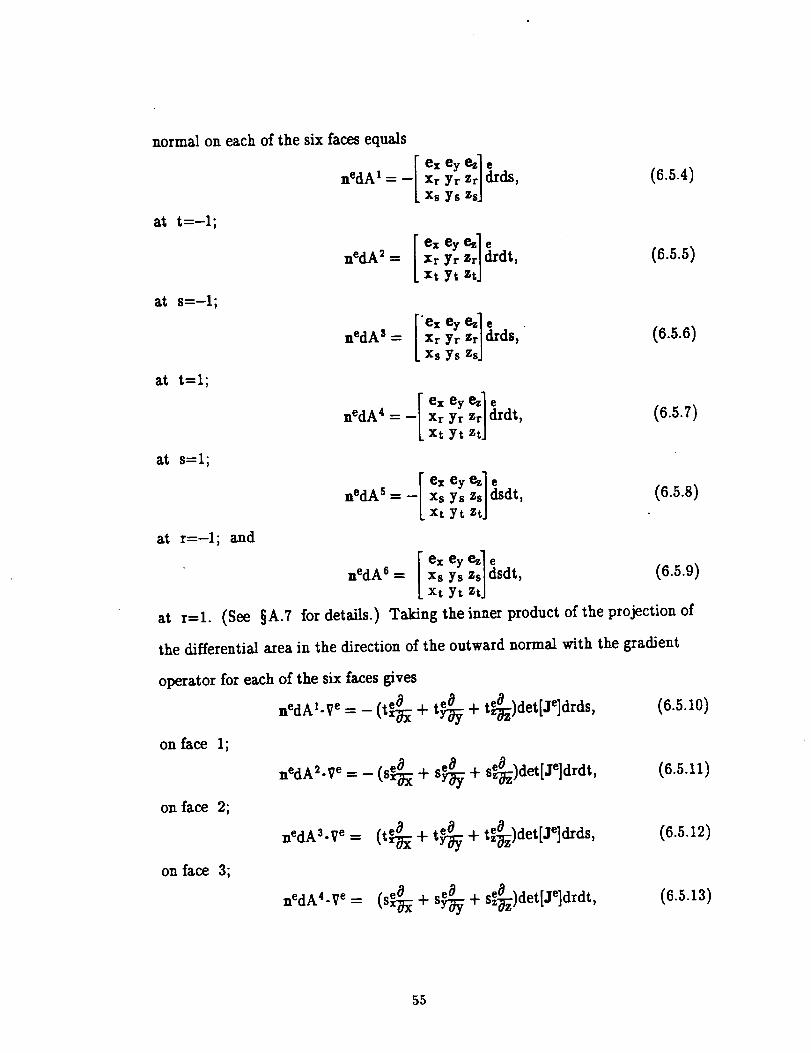
normal on each of the six faces equals

at t=-l;

at s--l;

at t-l;

I ex ey e_] enedA 1 = - Xr Yr z drds,

Xs Ys ZsJ

at s-l;

(8.5.4)

l ex ey !il enedA _ = Xr Yr drdt, (6.5.5)

xt Yt

"ex ey ze_rlenedA 3 = Xr Yr drds, (6.5.6)

Xs Ys ZsJ

at r=--l; and

at r=l. (See §A.7

ex ey e_] enedA 4--- XrYrZ drdt,

xt Yt ztJ

ex eynedA 5 = - Xs Ys Zs dsdt, (6.5.8)

xt Yt ztJ

[ "1eex eynedA _ - Xs Ys Zs dsdt, (6.5.9)

xt Yt ztj

for details.) Taking the inner product of the projection of

the differential area in the direction of the outward normal with the gradient

operator for each of the six faces gives

= _ (te#_-: +nedAl.Ve

on face 1;

on face 2;

on face 3;

nedA2.Ve - _ (sex_ +

nedA 3. ve =

nedA 4.Ve =

t_;; + te_z)dettJe]drds ,

s_d_ + Se_z)dettJe]drdt, (6.5.11)

(sex_ + s_ + Se_z)det[Je]drdt,

55

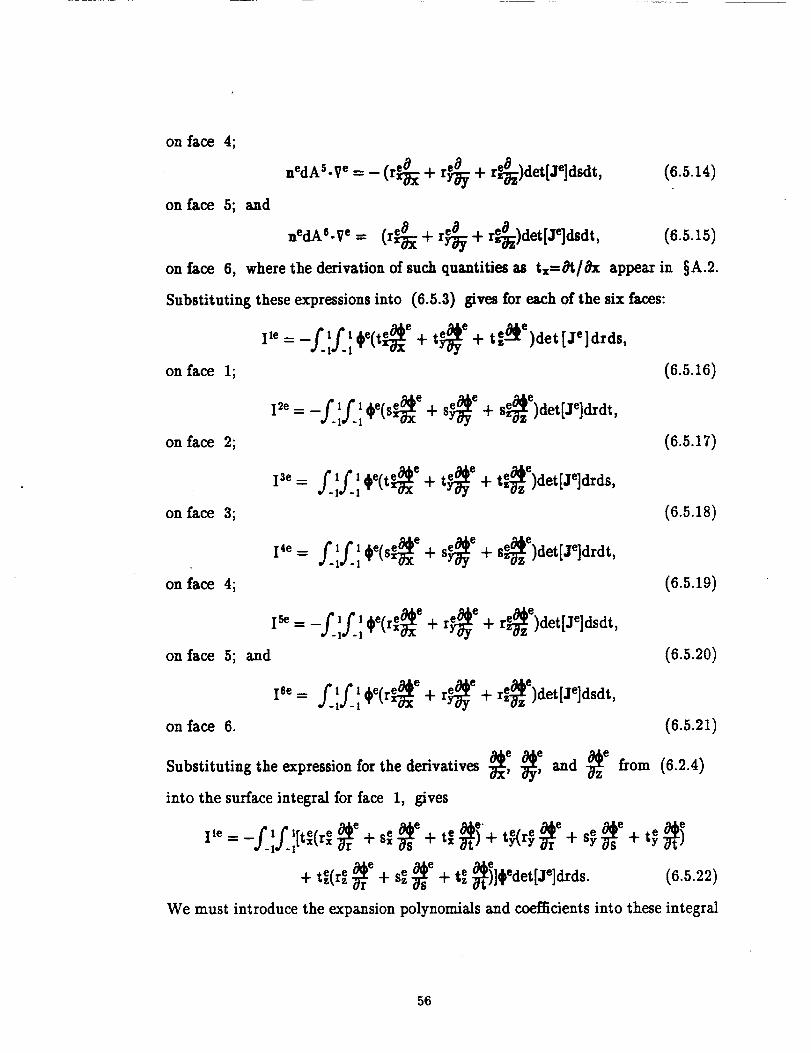
on face 4;

on face 5; and

nedA5, ve __.--(rex_ + r_d_ -i-rez_)det[Jeldsdt,

nedA°.Ve = (rex_ + r_d_ + re_)det[Je]dsdt,

on face 6, where the derivation of such quantities as tx-St/Sx

Substituting these expressions into (6.5.3) gives for each of the six faces:

1le-- -flf.' _e(tex_ e + t_d_ye + tze_e)det [Je]drds,

on face 1;

on face 2;

on face 3;

on face 4;

on face 5; and

I2e = -f.:f_: _e(se_ e + s_d_ e + Se_ze)det[Je]&dt,

I se= f.:f.: _e(te_xe + t_d_ e + t[_ze)det[Je]drds,

14e = f.:f_: _e(se_xe + S_y e + se_ze)det[Je]drdt,

+ r_y e + rez_ze)det[Je]dsdt,

1 1 e e eI',= f.f_, , + r y" + re_ze)det[Je]dsdt,

on face 6.

Substituting the expression for the derivatives

into the surface integral for face 1, gives

(6.5.14)

(6.5.15)

appear in §A.2.

(6.5.18)

(6.5.19)

(6.5.20)

I'e= £' £'rter-e _r e + se _s e + tze _ti+ t}(r} _r e + s} _se+ t_ _t i-J-1J- It x_-x

+ te(r e _r e + se _s e + tze _tilc}edet[Je]drds. (6.5.22)

We must introduce the expansion polynomials and coefficients into these integral

56

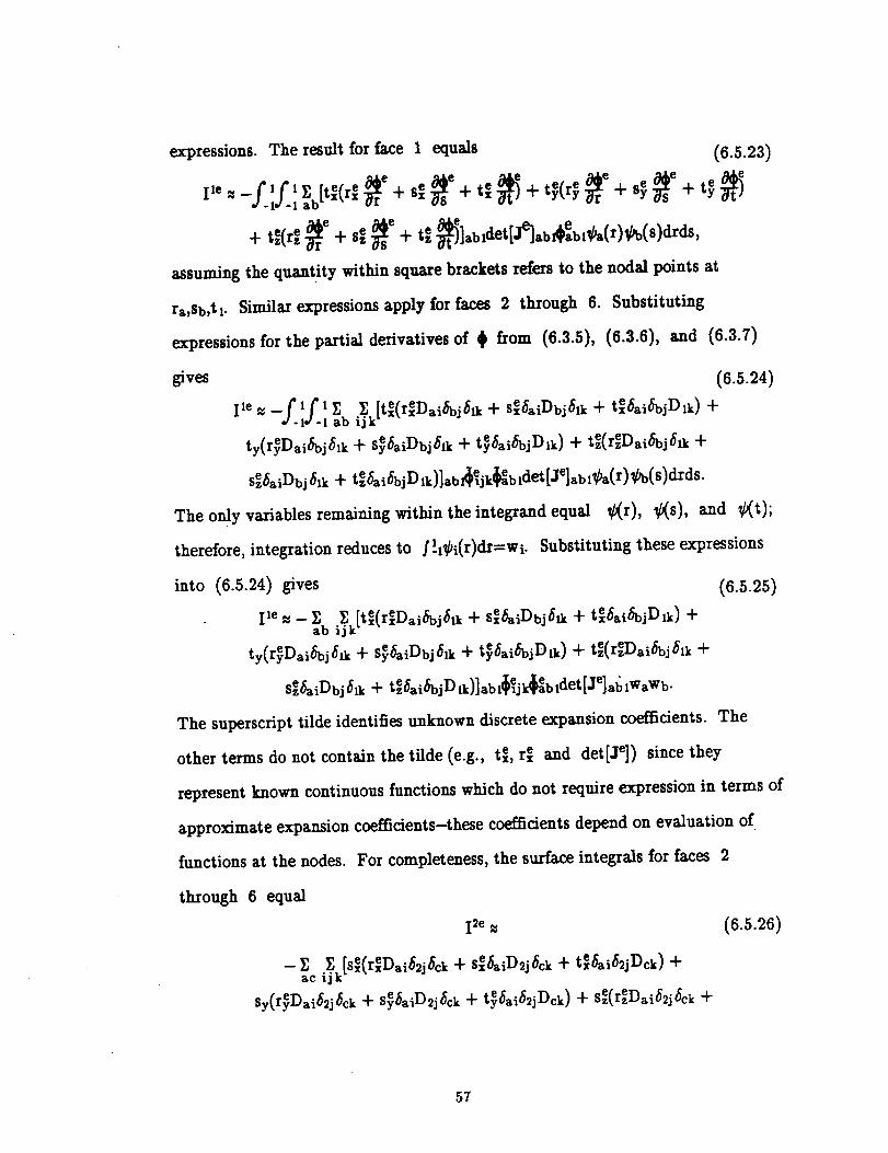
expressions.The result for face 1 equals (6.5.23)

"{" tze(re _e 4- sez _e+ tez _]abldet[je]ab1_eabl_a(r)_b(s)drd$,

assuming the quantity within square brackets refers to the nodal points at

ra,sb,t 1- Similar expressions apply for faces 2 through 6. Substituting

expressions for the partial derivatives of _ from (6.3.5),

gives

(6.3.6), and (6.3.7)

(6.5.24)

I'e_-f-:f-: _abi_k [txe(rxeDaiSbi6_ + se6aiDbj61k+ txe6aiSbjD1k)+

e ety(r_,Dai/_j_xk+ S_aiDbj_k + t_,6aiSbjD_k)+ tz(rzDai6bj6_k+

S_._Dbj6Zk+ t_&_b_Dzk)].b_jk_b_detIJe].bxf_(r)_(s)drds.

The only variablesremaining within the integrand equal _r), _s), and _t);

therefore, integration reduces to S l-t_i(r)dr=wi. Substituting these expressions

into (6.s.24) gives (6.s.2s)1 le _ - E E. [tex(reDai6bj61k + Sxe_aiDbj_lk + tex_ai_bjDlk) +

ab ij• ety(r_Dai_j_k+ s_aiDbj_ + t_a_jD_) + t,(r,D,_&j_k+

Sze_aiDbj_lk -[- te_ai_bjDtk)]ablCe_jk_aebldet[Je]al_lWaWb .

The superscript tilde identifies unknown discrete expansion coefficients. The

other terms do not contain the tilde (e.g., t e, re and det[Je]) since they

represent known continuous functions which do not require expression in terms of

approximate expansion coefficients-these coefficients depend on evaluation of

For completeness, the surface integrals for faces 2functions at the nodes.

through 6 equal

(_.5._)12e :

-- _ac i_k[se(reDai_2j_ck + Sxe_aiD2j_ck + te_ai_'jDck) +

eSy(rerDai_2j_ck 4- S_aiD2j_ck + t_ai_2jDck) -!- sz(r_Dai_j_c_ +

57

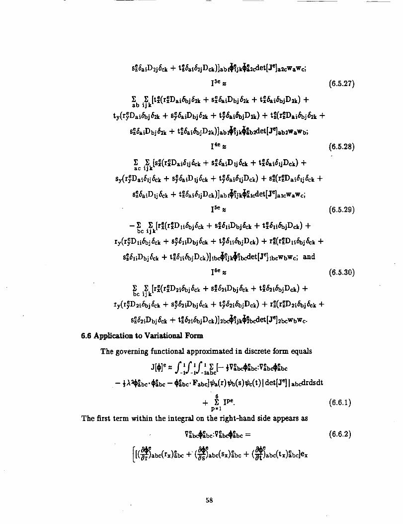
sze6aiD2j6ck + tez6ai62jDck)]ab_jk_cdet[Je]a2cWaWc;

13e

.._, [txe(rxeDai_oj62k + se6aiDbj_2k + te_ai6bjD2k) +a_b 1j_

ty(r_Dai6bj6_k + S_6aiDbj_2k + t_6ai_ojD2k) + te(reDai6bj62k +

S_Vbj6_k+ t_6._6bjD2k)].b_jk_b_et[Je].b_WaWb;

14e

se6aiDlj6ck + txe6si61jDck) +Y" i'k [sxe(rxeDai61j 6ck +ac j

Sy(r_I)ai_lj_ck + 8_aiDlj_ck + t_ai_ljDck) -[- se(rzeDai_lj_ck -_-

se_aiDlj_ck + te_ai_ljDck)]ab1_ejk_elcdet[JqalcWaWc;

15e

--Y, E [re(reDli6bj6ck -}- sex61iDbj6ck -}- tex_li_ojDck) +bc ij k

ry(r_D,_j6ck+ S_liDbj_ck+ t_61_bjDck)+ r_(r_D_6bj6_k+

sze61iDbj6ck + te61i_bjDck)]lbc_ejk_bcdet[Je]lbcWbWc; and

I ee

bc"_k [re(reD_i_bj_ck + se_iDbj_ck + te_i_bjDck) +

ry(r_D_i_bj_ck + S_iDbj_ck + t_i_bjDck) + re(rzeD_i_bj_ck +

8e_2iDbj_ck + tez_i_bjDck)]_bc_e_jk_]bcdet[Je]2bcWbWc.

6.6 Application to Variational Form

The governing functional approximated in discrete form equals

l 1 1

-- ½_ _bc" _ebc -- _bc" Fabc] _a(r) _b(S) _c(t) l det[Je] [ abc drdsdt

6+ _ I pe.

p=l

The first term within the integral on the right-hand side appears as

e e . e eVabAabc.VabAabc ----

[[(_iabc(rx)ebc +" (_siabc(Sx)ebc + (_tiabc(tx)_bc]ex

(6.5.26)

(6.5.29)

(6.5._o)

(6.6.1)

(6.6.2)

58

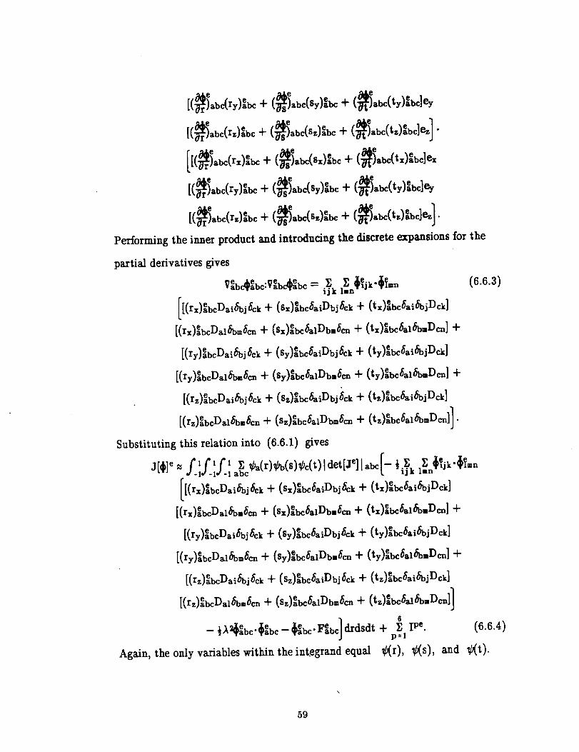
Performing the inner product and introducing the discrete expansions for the

partial derivatives gives

=[(rx)ebcDai_bj6ck + (Sx)aebc6aiDbj6ck + (tx)ebc_ai_bjDck]

[(rx)aebcDal6bm6cn + (Sx)ebc_alDbm6cn + (tx)aebc_l_buDcn] +

+ (ty)ebc6ai_ojDck]

+ (ty)esbc_aP_b, Dcn]+

+ (tz)aebc_ai_ojDck]

+ (tz)ebc_al_bmDcn]] •

[(ry)ebcDai_bj_ck + ($y)ehc_aiDbj_ck

[(ry)ebcD,_b._ + (sy)ebc_Db._

[(rz)ebcDai_bj_ck -}- (sz)ebc_aiDbj_ck

[(rz)ebcDal/_bm_cn + (sz)ebc_alDbm_cn

Substitutingthisrelationinto (6.6.11gives

j[¢]e m foily ":f Ii ab_c_a( r )_#b(S)_c(t )[ det [Je] [ abc [-- {i_k l_n _ejk "_mn

[[(rx)ebcDai_bj_ck + + (tx)ebc_ai_bjDck](sx)ebc_&iDbj _ck

[(_)_bcV_b._ + (S_)Ibc_Db-_ + (t_)Xbc_,_b-D_]+

[(ry)ebcDai_bj_ck + (sy)ebc_&iDbj_ck + (ty)ebc_&i_bjDck]

[(ry)ebcDal_m_cn + (Sy)eabc_alDbm_cn + (ty)ebc_al_ouDcn] +

[(r,)_b_D,_b_k+ (s,)ib_,_I)bj_k+ (t,)ib_,_ojI),k]

[(rz)eabcDal_bm_cn + (sz)ebc_alDbm_cn + (tz)eabc_alOCbzDcn]]

--½A2_ebc-_ebc--_ebc-F_abcldrdsdt + _ I pe.p=l

Again, the only variables within the integrand equal

(6.6.3)

(6.6.4/

_(r), _(s), _d _(t)

59

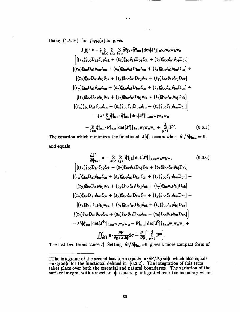
Using (1.5.16) for ll.l_i(x)dx gives

a[#le" - *,b_ci_k1._,_Jk'_'nIdet[aelI,b_W,WbWc

[[(rx)ebcDai6bj6ck + (sx)ebc_aiDbj6ck + (tx)_be6.i_jDck]

[(rx)ebcDal6bu6cn + (sx)ebe6alDbu6cn + (tx)ebe6al6b,Dcn] +

[(ry)ebcDai_bj_ck + (8y)ebc_aiDbj_ck + (ty)ebc_ai_bjDck]

[(ry)aebcDal6bu_cn + (8y)ebc6alDbu_cn + (ty)ebc_al_b,Dcn] +

[(rz)ebcDai_bj_ck + (sz)ebc_iDbj_ck + (tz)ebc_ai_bjDck]

[(rz)ebcDal_b._cn + (sz)ebc_alDb._cn -}- (tz)ebc_al_b,Dcn]]

6

-- Z _Tmn'F_mn [det[ael[ImnWlWmWn + Z Ipe.Iron p =!

The equation which minimizes the functional J[_] occurs when 6J/_Imn = 0,

and equals

_je_lun _ -- _ _ _eljkldet[Je]labcWaWbWcabc ij k

[(rx)aebcDai_bjtJck + (Sx)eabc_aiDbj_ck + (tx)ebc_ai_bjDck]

[(rx)%cDa16b,_cn + (sx)ebc6alDbm6cn + (tx)ebc6al6buDcn] +

[(ry)ebcDsi_oj_ck + (sy)ebc_aiDbj_ck + (ty)ebc_ai_vjDck]

[(ry)ebcDal(Vo._cn + (sy)ebc6alDbu6cn + (ty)ebc6al6buDcn] +

[(rz)ebcDai6bj_ck + (sz)ebc6aiDbj6ck + (tz)eabc6ai_bjDck]

[(rz)ebcDal_bm_cn + (sz)ebc_alDbu_cn + (tz)ebc_al6bmDcn]]

- A2_Tmn[ det[je] 1l_.WlW.W n - FT_n[ det[J_ 11..WlWfW. +

- - +i[ff_fl "Ugrad_ a° pffil

The last two terms cancel.$ Setting 5J/f_lffin-0

(6.6.5)

(6.6.6)

gives a more compact form of

_The integrand of the second-last term equals n-BF/_grad_ which also equals-n-grad_ for the functional defined in (6.2.2). The integration of this termtakes place over both the essential and natural boundaries. The variation of thesurface integral with respect to _ equals g integrated over the boundary where

6O

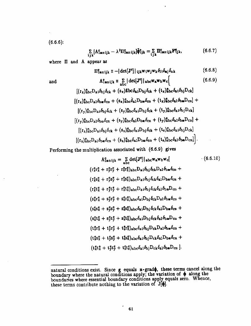
(6.6.61:

where II and A appear as

and

II_,nijk - -I det[Je] IijkWiWjWk_li_mj _nk

[(rx)aebcDai/_oj6ck + (Sx)Abc6&iDbj6ck + (tx)eabc_ai6bjDck]

[(rx)sebcDalSb-6cn -i- (Sx)ebc6alDb.6cn "I- (tx)sebc6al6b.Dcn] -{-

[(ry)aebcDai_oj_ck -{- (sy)ebc_aiDbj_ck -[- (ty)ebc_ai_bjDck]

[(ry)ebcDal_bm_cn + ($y)ebc_alDbm_cn + (ty)ebc_al_b.Dcn] -}-

J

+

(rxSxee -i- rySyee -i- rese)abcDai6bj6ck6sIDb.6cn-l-

(rxtxee + rytyee + rzetez)sbcDai6bj_ck_sl_.Dc_ +

ee ee(s,r_+ syry + S_ez)abc_aiDbj6ckDa16b.6cn+

(S_s_ee + SySyee + S_Sze)abc/_aiDbj6c_6aiDb.6cn+

ee ee(Sxtx+ +Syty szete)abc6aiDbj 6ck _&l _o.Dcn -t-

(txrxee + tyryee .i. t_e)abc_ai_bjDckDal_bm_cn .}.

(txSxee -{- tySyee + t_Sze)abc_ai6bjDck6alDb,_cn .4.

(txtxee _f tytyee + tzete)abc_ai_vjDck_alC_bmDcn ].

Performing the multiplication associated with (6.6.9) gives

A_fnijk = P" det[Je][abcWaWbWc[abc

e e e e r_ze)abcDai6bj6ckDal6b.6c_(rxrx + ryry -/-

(6.6.8)

(6.6.9)

natural conditions exist. Since g equals n-grad_, these terms cancel along theboundary where the natural conditions apply; the variation of _ along theboundaries where essential boundary conditions apply equals zero. Whence,

these terms contribute nothing to the variation of Jill.

61

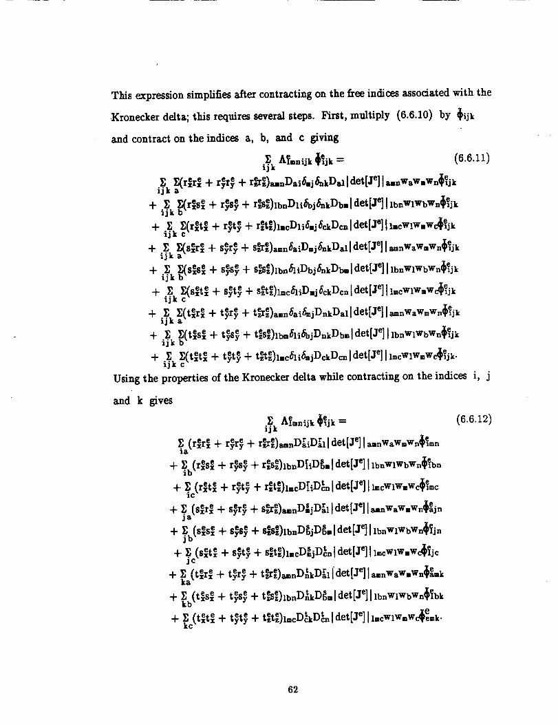
This expression simplifies after contracting on the free indices associated with the

Kronecker delta; this requires several steps. First, multiply (6.6.10) by _ijk

and contract on the indices a, b, and c giving

_zkAT..ijk_jk = (6.6.11)

ij_k a_rxe_e "}"ryryee + r_re)aanDai6.j_kDal[det[je] i amnWaW.wn_ejk

+ i_k b_rese + r_, + r_se)lbnDli_oj_nkDbu[ det[J e][ lbnW1WbWn_ejk

+ E cE(rxetxe+ r_t_ + r_e)l.cDli&j6ckDcn[det[Je][l.cWlW.,Wc_ejkijke e •

+ _k_(s_r'_÷ Syry+ S_,)_._6_D.j_.kV_xldet[J_]l,.w_w.wJ_jk-F i_k b_sese "4- S_ -_ s_se)lbn61iDbj6nkDbmldet[Je] IlbnWlWbWn_ejk

._. c_(Sxete + s_t_ + sete)lmcv_D_j6ckDcnldet[Je]ll.cWlWmWc_ejk1jk

tyry -_- t_re)amn&aiSmjDnkDa1[ det[Je] [amnWaWmWnC_ejk+ _ _terx e + eijk

+ ij_k bYa(txeSxe -I- t_S_ -F tese)lbmSliSbjDnkDbm[det[Je] [ lbnWlWbWn_ejk

+ iTk c_( tetxe + t_t_ + t_e)lmcSliSmjDckDcn Idet[J e]I lmcw]wmwJexjk.

Using the properties of the Kronecker delta while contracting on the indices i, j

and k gives

ijk

• ee ee e r r e e_" (rxrx -[- ryry _- r_z)amnDaiDal[ det[J ] I amnWaWmWn_mn

"i- _ib (resxe "4"r_rS_ -t- rese)lbnD_iD_ml det[Je] I IbnWlWbWn_ebn

• re e D t e e+ _c(retx e + r_t_ + ztz)lmcD_i cn[d t[J ]llmcWlWmwc_emc

e S. r

+ _a(Sxerxe + s_r_ + s_rz)aunDmjDalldet[Je] [aunWaWmWn_ejn

"["j_b(sxesex "{"8_ q- sesez)IbnD_jD_m[ det[Je] [ IbnWÂWbWn_jn

+ _c(Sextx e -I- S_t_ "t"setze)lmcI)SjDtnldet[Je] I lmcWlWmWc_jc

tyry + t_rz)amnDnkDal [det[Je] I amnWaWmwn_emk

t_Sz)lb_l)_kVi_,.Idet[J_]I_b_WlWbW_k"t" k_b(tesx e -I- t_s_ -I- e e t

ee ee D t t e+ _kc(tetxe + tyty + tztz)lmc ckDcnldet[J ][lmcWlWmwc_eemk.

62

The superscriptson D indicate the local direction associated with the

derivative. We must maintain this designation, since, in general, the number of

nodes in each of the three local directions differ. In other words, the quantities

D r, D s, and D t differ. A simplification occurs upon introduction of the

symmetric array of coefficients,

into

(6.6.13)(C 11)eaton --_

ee ee ee e(rxr= + ryry + r,.r,.)a=n Idet[J ]la=nWaW=Wn,

(C_2)_b_=ee ee(rxSx + r_, + rzSz)Ibn[det[Je][ IbnWlWbWn,

(C13)T,c-

e e e e rete_(rxtx 4- ryty "}" z zSl=c[det[Je][l=cWlW=Wc,

(C21)_=n=

ee ee ee t e(s,r, + syry+ s_,u)_=_lde [J][=_WaW.Wn,

(C_2)Tbn-

ee ee(SxSx+ s_s_ + SzSz)Ibnldet[Je]llbnWlWbWn,

(C23)_=c-=

e e e e szete)lmc[det[je][(Sxtx+ Syty + ImcWlWmWc,

(C3dhn-

ee ee e(txr_ + + [a_WaW.W_,tyry tzerz)amn [ det[J e]

(C32)_bn

(tes e + t_S_ + t_e)Ibnldet[Je][IbnWlWbWn,

and (C ss)_=c_- (6.6.21)

e e e e t=etze)l.cldet[Je]l(txtx+ tyty + ImcWlWmWc,

(6.6._2),_n_

_zAT=o_jk_,j==

(6.6.14)

(6.6.16)

(6.6.17)

(6.6.18)

(6.6.19)

(6.6.20)

63

ia e r. r e _ib(C,_)TbnD_iD_ebn +(Cn)amnDa_Dal_mn + .

(C_)_b.Dg_D_%n+ _(C2,)_,cD-_jD_#%c+jb

_ka(C 13)amnDnkDal_k +

_kc(C,,)_,,cDtkDt_..k.

Reordering the terms in this relation yields

i_kAU,_jk$',j_= (6.6.23)

e r. r e ja(Cl2e r s e. (Cn)unDa_Dal_xmn + r,. )afnDalDmj_ijn +la

e r t • _ib(Cl,)_bnD_.D_i_ebn "t"_(C_,).nD_ID_._ +.

_b(C_)Tb_D_jD_'$%°+ _b(C_')_bnD_'Dh$Tbk+t D' _c(C-,_)Ucck cJU_-D t D ¢ _. (C23)T-cDcn ,,j_jc + Dt Dt_cCC_)T.c_ h_.c+_c

Further arrangements produce

A_mnijk _%k ---- (6.6.24)ijk

e r e e D s e e t e_aCD_a)t[_i(Cn)amn(Dai_mn) + _ (C12)amn(.j_jn) 4- _k(Cl3)amnCDnk_amk)] +

_c_ (Ct3)Tmc(D[i_,c) + Z. (Cn)_.c(DSj_jc) + _k(Cs')_'c(Dtk_'k)]Dctn'$J

Introducing

and

and substituting into (6.6.24) gives

B_n = _.D_emn, (6.6.25)1

Ba_n_e - _.D-j_jn,S"e (6.6.26)J

- _k_._, (6.6.2_)ha_n - t e

:_The quantities within parentheses, for example Dai_ian, call be written as Aam

after performing the matrix multiplication. In this form the product DalAa_ndoes not satisfy the rules of matrix multiplication. In matrix multiplication thesecond index on Dal must equal the first index of Aa,,n. This involves

reorienting the indices of Dal by using the transpose. Hence the product should

be written as (Dla)tAamn, where the superscript t refers to the transpose.

64

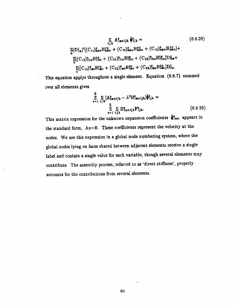
i_k A_.nijk _ejk =

t¢_ _e Bse e te+ +

b_[(Cl2)_bnB_gn + (C2_)_bnB_gn + (C23)_bnB_gn]D_,+

c_[(C,s)_-cB[ec + (C2s)_.cBTec + (C,,)T.cB_ee]Dt..

This equation applys throughout a single element. Equation (6.6.7)

over all elements _ves

E

e_=l ij_k[A_snij k -- _2II_.nijk]_ejk --

(8.6.28)

summed

E

l_kIl_snijk_jk -e=l ""

This matrix expression for the unknown expansion coefficients _.n appears in

the standard fore, Ax=B. These coefficients represent the velocity at the

nodes. We use this expression in a global node numbering system, where the

global nodes lying on faces shared between adjacent elements receive a single

label and contain a single value for each variable, though several dements may

contribute. The assembly process, referred to as 'direct stiffness', properly

accounts for the contributions from several elements.

65

REFERENCES

Korczak, K.Z. and Patera, A.T. 1986. An isoparametric spectral element method

for solution of the Navier-Stokes equations in complex geometry. J. Comp. Phys.

62:361.

Amon, C.H. 1988. Heat transfer enhancement and three-dimensional transitional

flows by a spectral-element-fourier method. Ph.D. Dissertation, Department of

Mechanical Engineering, Massachusetts Institute of Technology.

Wessel, R.G. 1992. Ph.D. Dissertation, Department of Mechanical and Aerospace

Engineering, Case Western Reserve University.

66

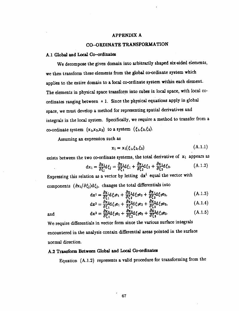
APPENDIX A

CO-ORDINATE TRANSFORMATION

A.I Global and Local Co-ordinates

We decompose the given domain into arbitrarily shaped six-sided elements,

we then transform these elements from the global coordinate system which

applies to the entire domain to a local coordinate system within each element.

The elements in physical space transform into cubes in local space, with local co-

ordinates ranging between • 1. Since the physical equations apply in global

space, we must develop a method for representing spatial derivatives and

integrals in the local system. Specifically, we require a method to transfer from a

coordinate system (x,,x_,xs) to a system (_b¢_,_s).

Assuming an expression such as

xi = (A.1.1)

exists between the two coordinate systems, the total derivative of xi appears as

Expressing this relation as a vector by letting dx i equal the vector with

components (_xi/_j)d_j, changes the total differentials into

dxt = _r_il_,e,+ _-_d2_2e,+ _sl _ses, (A.1.3)

dx' = _,el + _d_e, + _r_a _ses, (A.1.4)

and dxS = _dl _,e,+ _r_d_e, + _d_ses. (A.I.5)

We require differentialsin vector form sincethe various surface integrals

encountered in the analysiscontain differentialareas pointed in the surface

normal direction.

A.2 Transform Between Global and Local Co-ordinates

Equation (A.I.2) representsa valid procedure for transforming from the

67

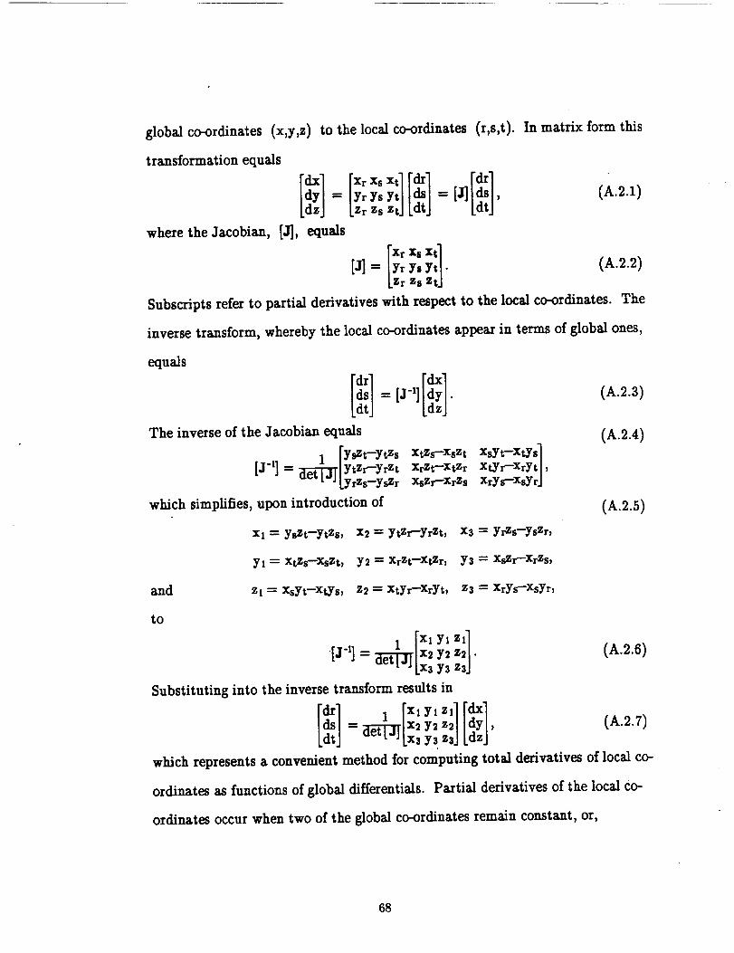
global co-ordinates (x,y,z) to the local co-ordinates (r,s,t).

transformation equals

dy - yrys y, = [_dz Zr Zs zt dt

In matrix form this

(A.2.1)

where the Jacobian, [J],equals

xt

[J]= Yry, y,. (A.2.2)Zr Zs Z

Subscripts refer to partial derivatives with respect to the local co-ordinates. The

inverse transform, whereby the local co-ordinates appear in terms of global ones,

equals

XtZs--XsZt xsYt--XtYs 1

XrZt--XtZr XtYr--XrYt],XsZr--XrZs XrYs--XsYrJ

[ii][d 1_ [j-l] l_zj"

The inverse of the Jacobian equals

I [yszt-ytzs

[j-l] = _]_j_/ytzr_yrz tlYrZs-YsZr

which simplifies, upon introduction of

X3 -- YrZs--YsZr,

YS -- XsZr--XrZs,

zs -- XrYs--XsYr,

(A.2.3)

(A.2.4)

(A.2.5)

and

to

xi = YsZt--YtZs, x_ = ytzr--YrZt,

yi "- XtZs--XsZt, Y2 "- XrZt--XtZr,

Zl -- XsYt--XtYs, Z2 -- XtYr--XrYt,

'[Jq] = _$']'[x] YsYszsZ_" (A.2.6)

Substituting into the inverse transform resultsin

lid,"I[11 [x, yl dx-- Z2

_-[_[Xx] y2yszs dY,dz (A.2.7)

which represents a convenient method for computing total derivatives of local co-

ordinates as functions of global differentials. Partial derivatives of the local Co-

ordinates occur when two of the global co-ordinates remain constant, or,

68

equivalently, by settingone or moreof the differential quantities dx, dy, or dz

equal to zero.

A.3 Volume Transformation

The variational form of the equations of motion contain volume integrals in

physical space; however, the expansion functions only apply in transform space.

Consequently, we require a transformation procedure for conversions between the

two systems.

If the vector dx i represents a differential length in the global system, a

differential volume equals

dV = dz1.(dz2,dz3).

Using the previously derived expressions for the vectors dx i gives

dV= eijk_d_i _d_j _d_k, (A.3.2)

equals the alternating unit tensor. Introducing the Jacobian gives

(A.3.3)

where eijk

dV = det[J]d_,d_gi_s;

where the determinant of the Jacobian depends on

det[J]d{,d{_3 = _iik_W_.I_ W_3 _id{jdfk

_ _(xl,x_,x3)_ j_ .2_ (A.3.4)- a(_1,_2,_3)_,_-_.

We require

0 < Idet[J]l < ® (A.3.5)

for a proper transformation. With (A.3.3) we have a method for transforming

volume integrals between the global and local c(>¢rdinate systems. This

transformation appears in the variational statement of the governing differential

equations, or whenever a volume integral in the global system appears.

A.4 Partial Derivatives

The governing differential equations require partial derivatives of the

69

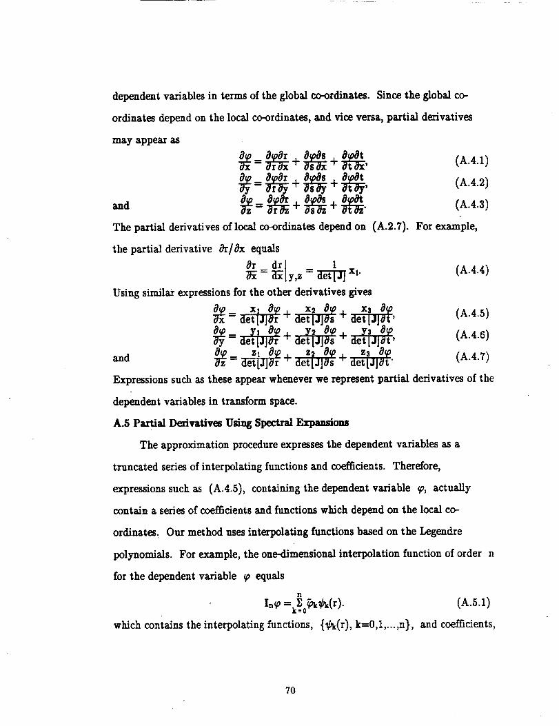
dependent variables in terms of the global co-ordinates. Since the global co-

ordinates depend on the local co-ordinates, and vice versa, partial derivatives

may appear as

The partial derivatives of local co-ordinates depend on (A.2.7).

the partial derivative _r/_x equals

y,z _ xl.

(A.4.2)

For example,

(A.4.4)

Using similar expressions for the other derivatives gives

_x = x, O_ _+_I_, (A.4.5)det [Jilt +

___at, (A.4.6)

and _z = _j_r + __S + _. (A.4.7)

Expressions such as these appear whenever we represent partial derivatives of the

dependent variables in transform space.

A.5 Partial Derivatives Using Spectral Expansions

The approximation procedure expresses the dependent variables as a

truncated series of interpolating functions and coefficients. Therefore,

expressions such as (A.4.5), containing the dependent variable _, actually

contain a series of coefficients and functions which depend on the local co-

ordinates. Our method uses interpolating functions based on the Legendre

polynomials. For example, the one-dimensional interpolation function of order n

for the dependent variable _ equals

n

In_ =k_0_Ck(r). (A.5.1)

which contains the interpolating functions, {g_,(r), k=0,1,...,n), and coefficients,

7o

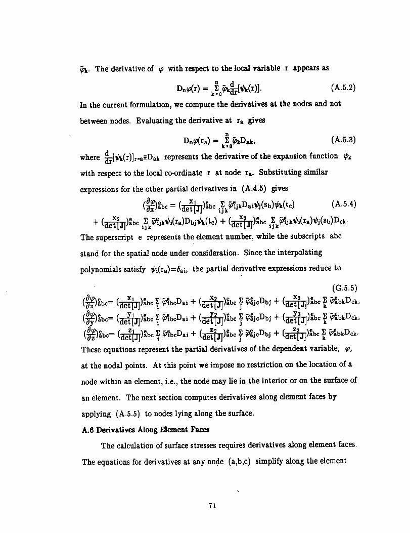
_. The derivative of _ with respect to the local variable r appears as

n dDn_r) = k_0_:[_Pk(r)]. (A.5.2)

In the current formulation, we compute the derivatives at the nodes and not

between nodes. Evaluating the derivative at ra gives

where _'[_(r)]r--a_Dak

with respect to the local co-ordinate r at node ra. Substituting similar

expressions for the other partial derivatives in (A.4.5) gives

n

Dn_ra) = k_f0_kDak, (A.5.3)

represents the derivative of the expansion function _

(A.5.4)

+ (_)ebc i_k_0_jk_i(ra)Dbj_bk(tc) -}- (_JI)aebc _Jg'_'"_e_jk_i(ra)_j(Sb)Dck"

The superscript e represents the dement number, while the subscripts abc

stand for the spatial node under consideration. Since the interpolating

polynomials satisfy _i(ra)=6ai, the partial derivative expressions reduce to

(G.5.5)

(_ 0)ebc-- (_-_J_)ebc _i _e_bcDai -b (_'_)ebc _ _jcDbj "b (_j])eabc _k _ebkI)ck'

(_ 0)eabc-_ (c_'FJ_)eabc _i _bcDal -b (_j])ebc _ _0_jcDbj "4- (_-_)aebc _k _eabkDck"

These equations represent the partial derivatives of the dependent variable, _o,

at the nodal points. At this point we impose no restriction on the location of a

node within an dement, i.e., the node may lie in the interior or on the surface of

an dement. The next section computes derivatives along dement faces by

applying (A.5.5) to nodes lying along the surface.

A.6 I)e.rivatives Along Element Faces

The calculation of surface stresses requires derivatives along element faces.

The equations for derivatives at any node (a,b,c) simplify along the element

71

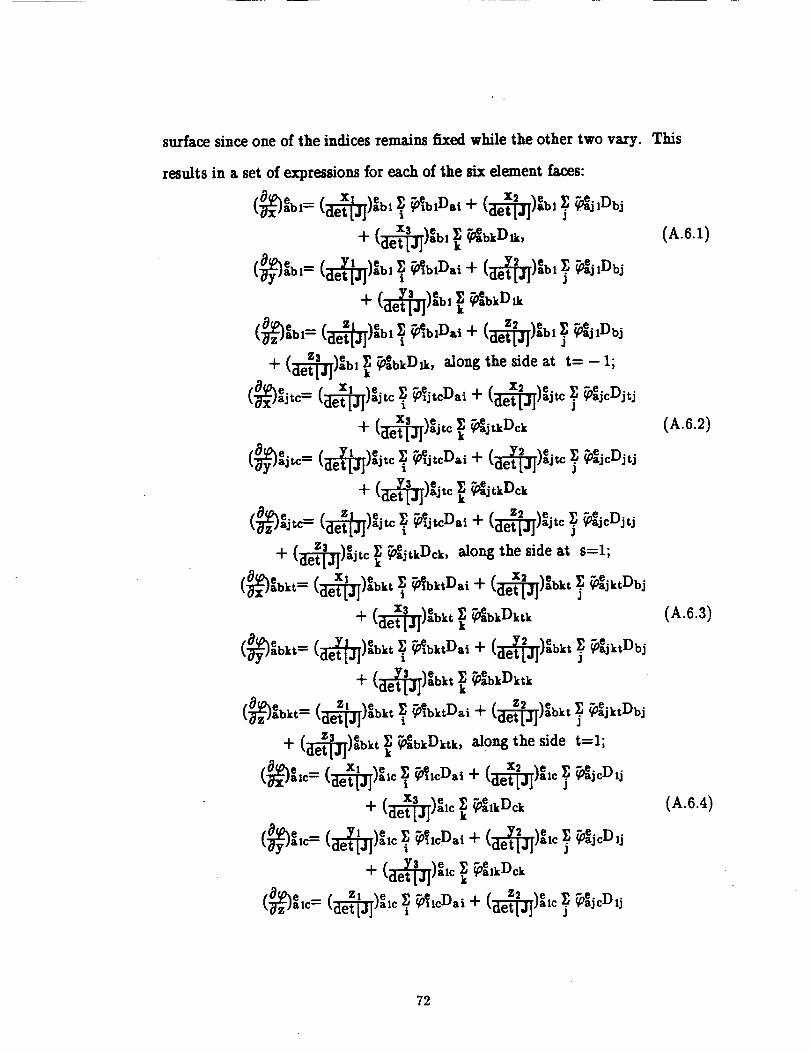
surface since one of the indices remains fixed while the other two vary. This

results in a set of expressions for each of the six element faces:

+ (_)_bl _ _bkD,_, along the side at t= - 1;

(_P)ejtc_.. [ Xl _e t" X2 _e. -e

/ X3 _e. t _jtkDck

4" (_)ejtc T _ejcDjtj

_ejtkDck

(_0)aejt c_ / Zl le. / z2 _e. -e D• _jc jtj_,_j_jajtc _i _jtcDai + I,_'_)ajtc

/ Z._ _e.

+ _-_ajtc k_ _ejtkDck, along the side at s=l;

(_ ebkt-_ (_)eabkt _i _elbktDai "_" (_)_bkt T _ejktDbj

"{- (_)eabkt k_

(_ebkt= (_)eabkt _i _bktDai

+ {(_ebkt-- (_J])ebkt _i _ebktDai

"[" (_)ebkt _k _ebkDktk'

_bkDktk

-{- (_-l_)ebkt _. _jktVbjJ

_ebkDktk

+ (_-_)ebkt _. _ejktDbjJ

along the side t=l;

/ x2 _e(_ezc'-" (_j])em _ _IcDai -I- ,_-F_jalc _ _oaejcD1j

+ (_)eic { m_kDck

+ (_)+,c _ _ea,kDck

(_O)ealc._/ Zl _e / Z2 _e _._ejcD1 j+

(A.6.1)

(A.6.2)

(A.6.3)

(A.6.4)

72

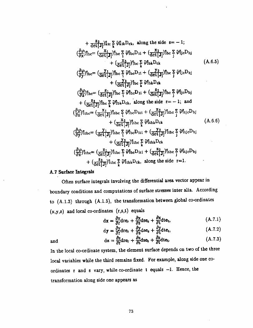
Z3 _e

+ _i)alc k_ _elkDck , along the side s-- - I;

(N_°-__c _._c_,,.(__c _._c_+ (_)_bc k__bkDck

_c= _)_bc __c_,_+I__ __c_+ (_)_o __b_D_

(_ _bc= (_I)_bc _i _bcD,i + (_i)_bc _ _jcDbj

-}- (_j_)_bc _k _bkDck, "along the side .r= - I; and

(_'_etbc= (_)e_tbc _. _ebcDiti + (_J_)etbc _. _etjcDbjj

_OetbkDck

"4- (_-_)etbc _. _etjcDbjJ

+ (_)e,bc k_ _tbkDck

_.c= __o __.cD_,+__c __c_._+ (_-_)etb c k_ _etbkDck , along the side r=l.

A.7 Surface Integrals

(A.6.6)

Often surfaceintegralsinvolving the differentialarea vector appear in

boundary conditions and computations of surface stresses inter alia. According

to (A.I.3) through (A.I.5), the transformation between globalco-ordinates

(x,y,z)and local co-ordinates (r,s,t) equals

dx = _-drer + _ises + _-dtet,

dy - _]Xer -l- _dses -I- _dtet,

_,-_e_+_s, +_,e_and

In the local coordinate system, the dement surface depends on two of the three

(A.Z.I)

(A.7.2)

(A.7.3)

localvariableswhile the third remains fixed. For example, along side one co-

ordinates r and s vary, while coordinate t equals -1. Hence, the

transformation along side one appears as

73

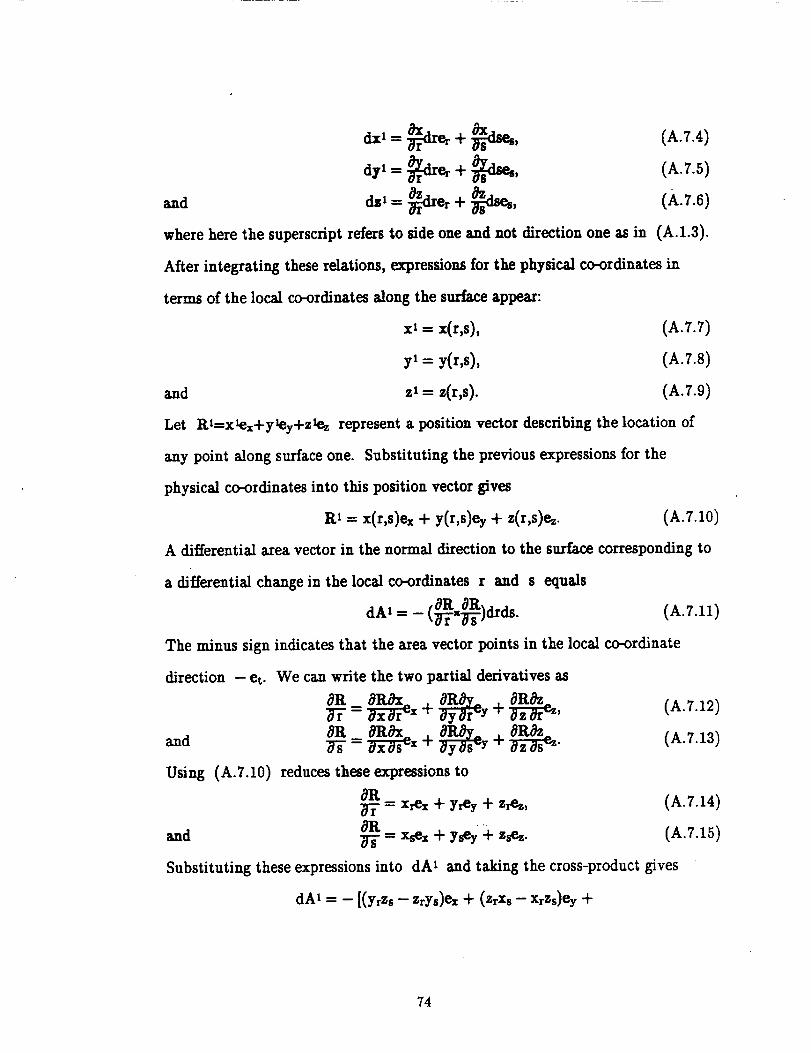
and

where here the superscript refers to side one and not direction one as in

(A.7.4)

(A.7.S)

(A.7.6)

(A.:.3).

After integrating these relations, expressions for the physical coordinates in

terms of the local co-ordinates along the surface appear:

_- _(r,s), (A.7.7)

y, = y(r,s), (A.7.8)

and zl --- z(r,s). (A.7.9)

Let Rt--xlex+y_y+Z_z represent a position vector describing the location of

any point along surface one. Substituting the previous expressions for the

physical coordinates into this position vector gives

R'-- x(r,S)ex + y(r,s)ey + z(r,s)ez. (A.7.10)

A differential area vector in the normal direction to the surface corresponding to

a differential change in the local coordinates r and s equals

,_TR 8Rx__j_ (A.7.11)dAl = - I._-"-_-]um_.

The minus sign indicates that the area vector points in the local co-ordinate

direction - et. We can write the two partial derivatives as

:taR=and _- + _-ey + _,_. (A.7.13)

Using (A.7.10) reduces these expressionsto

8R (A.7.14)_-- Xrex + y_y + Zrez,

_R (A.7.15)and _- = Xsex + ysey _-zsez.

Substituting these expressionsinto dAi and taking the cross-product gives

dA1 = -[(YrZs- ZrYs)ex+ (ZrXs- XrZs)ey"4-

74

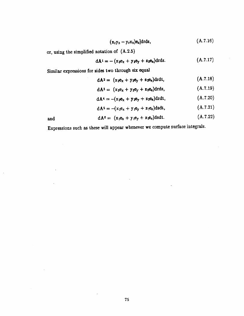
(XrYs--yrxs)ez]drds,

or,using the simplifiednotation of (A.2.5)

dA1 --- (x3ex + ysey + z_#.z)drds.

Similar expressionsfor sidestwo through six equal

dA2 - (x2ex + y_ey + z2ez)drdt,

dA3 = (x3ex + ysey + z3ez)drds,

dA4 ---(x_ex + y2ey + zg.z)&dt,

dAS = ---(xlex+ yley + zlez)dsdt,

and dA6 -- (xlex + yley + zlez)dsdt.

(A.7.16)

(A.7.17)

(A.7.18)

(A.7.19)

(A.7.20)

(A.7.21)

(A._.22)

Expressions such as these will appear whenever we compute surface integrals.

75

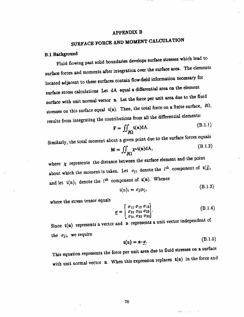
APPENDIX B

SURFACE FORCE AND MOMENT CALCULATION

B.1 Bartground

Fluid flowing past solid boundaries develops surface stresses which lead to

surface forces and moments after integration over the surface area. The elements

located adjacent to these surfaces contain flow--field information necessary for

surface stress calculations Let dA

surface with unit normal vector n.

stresses on this surface equal t(n).

equal a differential area on the element

Let the force per unit area due to the fluid

Then, the total force on a finite surface, _t2,

results from integrating the contributions from all the differential elements:

F = __/f&t(n)dA. (B.I.I)

Similarly,the totalmoment about a given point due to the surfaceforcesequals

M--- _'f _t(n)dA, (B.1.2)n

where X represents the distance between the surfaceelement and the point

about which the moment istaken. Let cji denote the ith component of t(j),

and let t(n)i denote the ith component of t(n). Whence

t(n)i- 0.jinj, (B.1.3)

where the stress tensor equals

0"11 0"12 0.131a_l a_ 0._a|- (B.1.4)0.31 0.32 0.33J

n represents a unit vector independent of

w

Since t(n) represents a vector and

the aji, we require

t(.)= n-_a. (B.I.5)

This equation representsthe forceper unit area due to fluidstresseson a surface

with unit normal vector n. When thisexpression replaces t(n) in the forceand

76

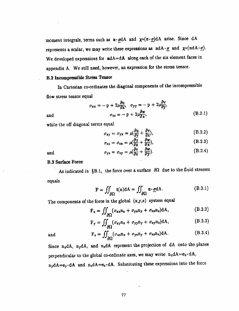
moment integrals, terms such as n.__lA and x_(n-_.)dA arise. Since dA

represents a scalar, we may write these expressions as ndA-£ and x_(ndA-_.

We developed expressions for adA--dA along each of the six element faces in

appendix A. We still need, however, an expression for the stress tensor.

B.2 Incompressible Stress Tensor

In Cartesian co-ordinates the diagonal components of the incompressible

flow stress tensor equal

__ 2_vaxx=-p+2#_x, ayy -p+ #_:,

azz = - p + 2_z, (B.2.1)and

while the off diagonal terms equal

and

B.3 Surface Force

As indicated in §B.1,

equals

(rxy= _ryx=#(_'{-_),

• o%vO'yz = O'zy /_(_Z "{- _').

the force over a surface 0fl

(B.2.2)

(B.2.3)

(B.2.4)

due to the fluid stresses

F=ff =fffl ""_fl -

The components of the force in the global (x,y,z)

and

Since nxdA, nydA,

perpendicular to the global co-ordinate axes, we may write nxdA=ex-dA,

nydA=ey-dA and nzdA=ez-dA. Substituting these expressions into the force

system equal

Fx = __f/_n(_xxnx+ ayxny + _rzxnz)dA, (B.3.2)

Fy = __ff_fl(gxYnx+ ¢ryyny+ azynz)dA, (B.3.3)

F, = ffm(ax,nx + Cryzny + crzznz)dA. (B.3.4)

and nzdA represent the projection of dA onto the planes

77

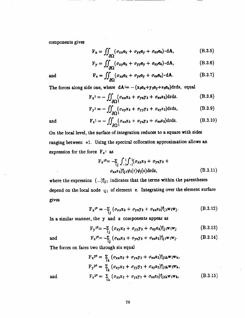
components gives

and

Fx -- ffafl(oxxex + oyxey + osxez)-dA,

Fy - :f_ (oxyex + oyyey + osyez)-dA,

F_ = f_n(o,,e_ + oy_ey + o_e._)-dA.

(B.3.5)

(B.3.6)

(B.3.7)

equal

(B.3.8)

(B.a.0)

The forcesalong side one, where dA1= - (xsex+ysey+zsez)drds,

Fx i = - :_ !_xxX_ + -yxY3 + osxz,)drds.n

::,!------ UxyX3 4- ¢ryyys-F O'zyzs)drds,FYl n

and Fz I - -f_, (uxzxs + Uyzys % czzzs)drds. (B.3.10)8nl

On the local level, the surface of integration reduces to a square with sides

ranging between _1. Using the spectral collocation approximation allows an

expression for the force Fx 1 as

.. 1 1Fx le-"-Y, _.l__,(o'xxxs-I-uy_ys %zj

u,xz3) j1 i(r) j(s)drds, 11)

wheretheexpression(.-.)_jlindicatesthatthetermswithintheparentheses

depend on the localnode ij_.ofelement e. Integratingover the element surface

gives

Fx le - -E.. (UxxXs + Uyxys + tyzxzs)_jlWiWj. (B.3.12)lJ

In a similar manner, the y and z components appear as

Fy le'--_.. (OxyXs "{"O'yyys _- _rzyZs)_jlwiwj (B.3.13)ij

and Fz re: -_.. (O'xzXS -[" _ryzYS + O'zzZS)_jlWiWj. (B.3.14)1j

The forces on faces two through six equal

Fx_e - _ik (_rxxx2 "_ UyxY2 % GrzxZ2)ejtkWiWk,

Fy_e - _ik (_xyX2 q- Cryyy2 -F _rzyZ2)eljtkWiWk,

and Fz2e"- _' (_rxzX2_" CryzY2-f O'zzZ2)e_jtkWiWk, (B.3.15)ik

78

on face two, where dA=(x2ex+y2ey+z_)drdt;

Fx 3e = _.. (_xxXs + CryxYs + ffzxV.3)xejktWiWj,ij

Fy se -- _.. (UxyXS + O'yyys + GzyZ3)_jktWiWj,lj

and Fz 3e = _.. (_rxzx3 -[- Gyzys + o'zzz3)exjktWiWj,1j

on face three, where dA=(xsex+Ysey+zse_)drds;

Fx4e - _ik (UxxX2 + _yxY2 + u=z_)elxkWiWk,

Fy4e = _ik (UxyX2 + "O'yyy2+ GzyZ2)_lkWiWk,

and Fz4e = _k (CrxzX_ + uyzy2 + _rzzZ_)_lkWiWk,

on face four, where dA= - (x2ex+y2ey+z_)drdt;

Fx se = _ (UxxXl + uyxyl + GzxZl)_jkWjWk,jk

PYre= ( xyxl + uyyyl+ .',) jkWjWk,

and FzSe -" _k (GxzX, + GyzYl + ffzzZl)_jkWjWk,

on face five, where dA--- - (Xlex+yley+zlez)dsdt; and

FxSe = I] (u_xxl + uyxyl + _,._zl)_tjkWjWk,jk

Fy6e - _k (ffxyXl + O'yyy! + O'zyZl)_tjkWjWk,

and Fz 6e - _ (ffxzXl + ffyzYl + ffzzZl)e_tjkWjWk,jk

on face six, where dA-(xlez+yley+zlez)dsdt. Note that when any of the

subscripts ijk equals 1, we refer to the node at the face corresponding to rat

equal to -1, and when any of the ij_ equals it, jt, or kt, we refer to the

node at the face corresponding to rat equal to 1. Also, the basis functions

integrated over the local co-ordinate domain, wi_=f.l_i(r)dr, wj=/_xl_j(s)ds ,

and Wk-f11_i(t)dt , differ when the number of nodes in the r, s, or t

directions differ; consequently, we must remember that wi refers to the r-

direction, wj refers to the s-direction, and Wk refers to the t-direction.

(B.3.16)

(B.3.17)

(B.3.18)

(B.3.19)

B.4 Surface Moment

79

The moment along a surface due to the fluid stresses appears as

M =/'/" x_n-adA, (B.4.1)-

where the moment "arm" equals X=xxex+Xyey+XLez. Substituting into (B.4.1)

and performing the cross product yidds the moment components in the global co-

ordinates as (B.4.2)

Mx = __ffRfl[XY(_xznx -1- (ryzny -i- (rzznz) -- Xz(_xynx -i- _ryyny -}- _zynz)]dA,

My "- :f_i_ [Xz(Crx=nx -1- ayxny + azxnz) - Xx(_x_nx + O'yzny + _zznz)]dA,

Mz = ff0 [Xx(axynx -F _yyny + azynz) - Xy(_rxxnx q- _yxny -}- azxnz)]dA.

Using the same notation as in the surface force calculation gives

Mx- __ffRi2[Xy(axzex + Cyzey + a_zez)- Xz(Cxyex + (ryyey + Czyez)]-dA,

My -- __ff_n[Xz(_xxex + _yxey -_- ffzxez) -- Xx(O'xzex -{- O'yzey -]- O'zzez)]-dA,

M, = vff_[xz(_zYe_ + ayyey+ _,_) - Xy(_xe_ + ay_ey+ _,_)]-di.(B.4.3)

For example, the x-component evaluated along side one, where

dA=-[xse=+y sey+zsez]drds, equals

Introducing the spectralexpansion functionsgives

M:= + ,,,,s, (s.4.4)+ ffzzZ3) -- Xz(CYxyX$ "F (ZyyY3 -F ffzyZ3)]ejl_bi(r)_bj(s)d_ds.

After integration we obtain

Mz_= -_.. [Xy(U_xs+ ay,S3+ a_za)D

-- Xz(O'xyX3 + ¢ryyys "t- _rzyZ3)]ejlWiWj.

In a similar manner, the y and z components appear as

(B.4.5)

8O

My le = -E.._j

M.le = __olj

The moments

Mx_e -

My2 e -

Mz2e -

along face

Mx3 e =

My3e --

Mz3e --

along face

[x.(_xxx3 + _y_y3+ a,_z3)- xz(_x,x3 + _y_y3+ _.,_3)]_jlwiwj,

[Xx(axyX3 + O'yyy3 + O'zyZ3) --Xy(_rxxX3 + ay-xY3 + a_zzs)]eljlwiwj.

along faces two through six equal

_ik

y_ik

two, where dA=(x2ex+y2ey+Z_.z)drdt;

[_y(GxzX2 "_- Gryz.V2 "[- ¢TzzZ2) -- _z(axyX2 4" O'yyY2 _" _zyZ2)]ejtkWiWk,

[_z(CTxxX2 + O'yx.V2 _" O'zxZ2) -- _x(CYxzX2 "1- _ysY2 + crzzZ2)]ejtkWiWk,

[xx(_zyX2+ ayyy_ + a.yZ2) - Xy(_._x_ + _y_y2+ _--z_)]ejtkWiWk,

(B.4.6)

_.. [Xy(CTxzX3 + ayzy3 -t- _rzzZ3) -- Xz(CTxyX3 + ¢TyyY3+ _rzyZ])]ejktWiWj,ij

_.. [x_(_x.X, + _y_y3+ _._z,)- x_(_,x3 + _y_y3+ _._3)]_jktW_Wj,_J

_. [_(_yX_ + _yyy_+ _zyZ,) - _y(_x_ + _y_y, + _z_)]e_ktWiWj,_J

three, where dA=(x_ex+yzey+zsez)drds; (B.4.7)

Mx4e = --_ik [Xy(_zzx2 + ¢ryzy2 + _zzZ2)- _z(_TxyX2 4" _yyY2 + _TzyZ2)]elkWiWk,

My4e= --_k [_z(O'xxX2 + ¢TyxY2 + _TzxZ2)- _x(CTxzX2 _- O'yzy2 "[" ¢TzzZ2)]elkWiWk,

Mz4e "" --_ik [Xx(CrzyX2 + O'yyY2 + _rzyZ2) -- Xy(O'xxX2 + ¢ryxY2 + ffzxZ2)]etkWiWk,

along face four, where dA= - (x2ex+y2ey+z_)drdt; (B.4.8)

Mx 5e = -_ [Xy(CrxzXl + O'yzy! -t- O'zzZl) -- Xz(O'xyXl-{- ¢Tyyy. l -I- O'zyZl)]_jkWjWk,jk

My 5e - -Y_ [Xz(_rxxxl + O'yxYl "_" O'zxZl) -- Xx(axzXl "}"O'yzYl + _TzzZl)]_jkWjWk,jk

_,_e = __ [_(_yx_ + _yyyl + _,yZ_)- _y(_,_x_ + _y_y_+ _z_)]_j_w_w_,jk

along face five, where dA= - (x_ex+y_ey+z_z)dsdt; (B.4.9)

Mx_ e =

My8 e :

Mz _e =

along face six, where dA---(X_ex+y_ey+ztez)dsdt.

_k [XY(O'xzXI _" _ryzYl + _rzzZl)- Xz(0"xyXl + O'YyYl + ¢TzYZl)]etjkWjWk'

[Xz(_rxxXl -l- _73rr.y I "[- _TzxZl)- Xx(ffxzX 1 + ¢ryzYl -{- ¢rzzZl)]extjkWjWk,jk

_k [_x(_TxyX1 "_ UyyYl -_- UzyZl)- _y(_TxxXl _- CryxYl -J- (TzxT.l)]eltjkWjWk,

(B.4.10)

81

APPENDIX C

IMPERMEABLE WALL BOUNDARY CONDITIONS

C.1 Physical Basis

Along an impermeable wall the normal fluid velocity must equal the normal

component of the wall velocity, while the tangential velocity may vary. We

express this as

n-V = n-Vwall. ((].1.1)

Another condition on impermeable wall boundaries requires zero tangential

stress, or, equivalently, that the stress points normal to the surface. In other

words, the cross product of the surface unit normal and the local stress vector

equals zero. Thus, an impermeable wall, unlike a solid wall, cannot support a

tangential stress. In symbolic form this boundary condition equals

= 0, (c.1.2)

where n represents the surface outward unit normal vector, and _u represents

the total stress tensor consisting of the sum of the isotropic and deviatoric terms.

We must prove that the combination of these two boundary conditions equals the

single condition given by

(n-V)V = 0. (C.2.1)

The derivation of thisrelationfollows.

C.2 Mathematical Derivation

Begin by expressing the unit normal as

n = nxex + nyey + nzez (C.2.2)

and the velocity as

V = Uex + Vey + Wez.

The inner product n'V gives

82

n-V = Unx + Vny + Wnz. (C.2.4)

Setting this equal to the normal velocity of the boundary gives

Unx + Vny + Wnz = n'Vwall. (C.2.5)

The stressvector on a surfacewith normal, n, equals t(n) which appears as

t(o)= _..n= (c.z0)

(o'xxnxJr O'yxny % _rzxnz)ex Jr

(azynx+ ayynz+ _,yn,.)ey+

(ax_nx+ _y_ny+ az,n,)e_

according to appendix B. The crossproduct ofthisrelationwith the unit normal

equals

nxt(.)= ___.n= (c.2.7)

[ny(_rxznx + ffyzny Jr O'zznz) -- nz(Crxynx Jr #yyny + Crzynz)]ex Jr

[nz(axxnx + ayxny + azxnz) -- nx(cxznx + ayzny + azznz)]ey +

[nx(axynx Jr O'yyny + O'zynz) --ny(O'xxnx + O'yxny + O'zxnz)]ez.

Using (B.2.1) through (B.2.4) for the stresscomponents gives the following

relationsfor the three components of the above expression:

,SUI#-W _N¢(_x..n)x--_nxnyt#z,_x)+_nyny(#yI_)+_ny(2_-p)-

n .aU oW. n "2°W" ]mznz(#_z_ 6W"- _ny_t _- (c.2.8)(nxo-.n)y _U n ,_U_ o_V 8W • 8U/_

=/_xnzC2_-p) +/_ny Z(#y, #x ) +/_n_nz(#x ,az/

n ,0U, OW, n ,#--W_#_zz) 2_TV'- -_zn_(_-_--p), (c.2.9)_IIx x(#z, _X } ]_[lyXtSy ,

• _U_aV ' n /2 _V- 8W_(n,__-n)_= _n_t#y, #_) + _-y _ _y P)+ _X(#y, _)-

aU _/ aU _nzny(_rz _ _tz (C.2.10)/atxny(2_-_- p) --/_lyny(_--F_-) - # y ).

The pressure terms cancel in each of these expressions giving

(n_o'-n)x-' n _U o_V _W _V ,2_W _V

ow av _w (c.2._1)_,n,(_ + #_-)- _n,(_- + _-_-),

83

"2aU + av aw(nx_a-n)y = pnx z_, _--- _-) + pnznz(_-_- +

o%V _vV oW), (C.2.12)_xnx(_zU + _-) - _ynx(_- + _-

_v)_(nxo'-n)z ----/mxnx(_y + _---_x)+/mynx(2_y- 2_x ) +/mznx(_-y + _-

8U _/mz, ny(_ z + 8W (C.2.13)]_Ilyny(_ X q" _') _'_-)"

After furtherrearrangement we obtain

"nSU nSV nSW" -nSU n_Tz )y_-/+(n_-n)x =-_nz( x_ + %+ _)+/my( x_+ n 8V

+ _(nx_ + ny_ + nz_)(nyW - nzV), (C.2.14)

"n 8U n _ n 8W) "n 8U n 8V n o'rW"(n-o'-n)y=-/_nx( _+ _+ _ +_nz( _+ _+ z-,d_)

+ _(nx_ + ny_ + n_z)(nzU- nxW), (C.2.15)

n _¢" n _ , tnSU n _ n 8W(n,,__-n),= __y(n_..U_.+ y._ + ,_.) + ,,.,xt _ + _ + _,_-)

+/_(nx_ + ny_ + nz_)(nxV - nyU). (C.2.16)

The partial derivatives of the unit normal vector with respect to the spatial co-

ordinates differ from zero on a curved surface. Hence, we cannot interchange the

derivative operator in the first two terms of each expression with the components

8U o_ o_q _-(nxU nyV nzW)).of the normal vector (e.g.,nx_--l-ny_-q-nz-,d- _- _ + +

However, the derivativemay move outside the components of the normal vector

if we only consider surfaces with zero curvature. When we restrict ourselves to

thiscase,the above relationsmay appear as

(nxo'-n)x = -_-{nxU + nyV + nzW)+/_ny_nxU + nyV + nzW)

+ _n_ + ny_ + nz_z)(nyW - nzV), (C.2.17)

(nxz-n)y- -/_nx_nxU + nyV + nzW)+/mz_nxU + nyV + nzW)

+ _(nx_ + ny_ + n_z)(n,U - nxU), (C.2.18)

(nx__-n)z- -/_ny_nxU + nyV + nzW)+/mx_nxU + nyV + nzW)

+ _(n_ + ny_ + n_z)(nxV - nyU). (C.2.19)

Introducing n-V=nxU+nyVTnzV and n-V--nx_ny_n_z into these

84

expressionsyields

(nx o'-n)x--- l*t"[n_0 nz_j:!0_n- V + _- V(nyW-nzV), (C.2.20)

(nx__-n)y = -_(n_z nz_)n.Y + _.V(nzU-nxW), (C.2.21)

= + --vcnxV-nyU). (C.2.22)After introducing the cross product, the three components of (n=o'-n) reduce to

a single vector expression given by

(n-__-n)= _[(n.V).-V + (n-V)n=V]. (c.2.23)

This equation also appears as

(n,K-n) = _,[V(n-V) + (n-V)V]. (C.2.24)

Introducing n-V=n-Vwall gives

(nx_.n) = //-Ux[V(n-Vwall) -_ (n.V)V]. (C.2.25)

For a general curved boundary moving with velodty Vwan, the quantity

V(n-Vwall), does not equal zero. However, since we are limiting our

consideration to fiat boundaries, this term does equal zero. In this case the

boundary condition reduces to

(n=__..)= _.=[(n-V)V]. (c._.2s)

Since the original boundary condition, n-_u-n, equals zero, we require

_.=[(n-V)V]= _(..v)(..v) = o. (c._..gz)

This equation is satisfied when the unit normal lies parallel to the velocity vector

giving n=V--O. This seems like a most unusual condition and we assume that it

does not hold for most boundaries. The other possibility requires

(n-V)V = 0, (C.2._-8)

and represents the desired form of the boundary conditions given in §C.1. This

proves that the two impermeable wall boundary conditions reduce to

homogeneous natural conditions when we enforce (1) zero surface curvature to

85

ensure V(n-Vwall)=O, and (2) a surface with unit normal not parallel to the

local velocity.

86

Form Approved

REPORT DOCUMENTATION PAGE OMB NO. 0704-0188

Public reportingburdenfor this collectionof informationis estimated to average 1 hour per response, including the time for reviewinginstructions,searching existing data sources,gatheringand maintainingthe data needed, and completingand reviewingthe collectionof information. Send comments regardingthis burden estimateor any other aspect of thiscollectionof infownation,including suggestionsfor reducingthis burden, to WashingtonHeadquarters Services, Directoratefor Information Operations and Reports, 1215 JeffersonDavis Highway.Su=te1204. Arlington.VA 22202-4302, and to the Office of Managementand Budget, PaperworkReductionProject(0704-0188), Washington. DC 20503.

1. AGENCY USE ONLY (Leave blank) 2. REPORT DATE 3. REPORT TYPE AND DATES COVERED

April 1993 Technical Memorandum

4. TITLE AND SUBTITLE

Incompressible Spectral-Element Method--Derivation of Equations

6. AUTHOR(S)

Russell G. DeAnna

7. PERFORMING ORGANIZATION NAME(S) AND ADDRESS(ES)

NASA Lewis Research Center

Cleveland, Ohio 44135-3191

and

Vehicle Propulsion Directorate

U.S. Army Research Laboratory

Cleveland, Ohio 44135-3191

9. SPONSORING/MONITORING AGENCY NAME(S) AND ADDRESS(ES)

National Aeronautics and Space Administration

Washington, D.C. 2054.6--.0001and

U.S. Army Research Laboratory

Adelphi, Maryland 20783-1145

5. FUNDING NUMBERS

WU-505--62--OK

1L161102AH45

PERFORMING ORGANIZATION

REPORT NUMBER

E-7758

10. SPONSORING/MONITORING

AGENCY REPORT NUMBER

NASA TM-106109

TR-92-C-022

11. SUPPLEMENTARY NOTES

Responsible person, Russell G. DeAnna, Propulsion Directorate, U.S. Army Research Laboratory, (216) 433--3385.

12a. DISTRIBUTION/AVAILABIUTY STATEMENT

Unclassified - Unlimited

Subject Category 34

12b. DISTRIBUTION CODE

13. ABSTRACT (Maximum 200 words)

A fractional-step splitting scheme breaks the full Navier-Stokes equations into explicit and implicit portions amenable to

the calculus of variations. Beginning with the functional forms of the Poisson and Helmholtz equations, we substitute

finite expansion series for the dependent variables and derive the matrix equations for the unknown expansion coefficients.

This method employs a new splitting scheme which differs from conventional three-step (non-linear, pressure, viscous)

schemes. The non-linear step appears in the conventional, explicit manner, the difference occurs in the pressure step.

Instead of solving for the pressure gradient using the non-linear velocity, we add the viscous portion of the Navier-Stokes

equation from the previous time step to the velocity before solving for the pressure gradient. By combining this "pre-

dicted" pressure gradient with the non-linear velocity in an explicit term, and the Crank-Nicholson method for the viscous

terms, we develop a Helmholtz equation for the final velocity.

14. SUBJECT TERMS

Numerical; Spectral-element method; Computational fluid dynamics

17. SECURITY CLASSIFICATION

OF REPORT

Unclassified

NSN 7540-01-280-5500

18. SECURITY CLASSIFICATIONOF THIS PAGE

Unclassified

19. SECURITY CLASSIFICATIONOF ABSTRACT

Unclassified

15. NUMBER OF PAGES

8816. PRICE CODE

A0520. LIMITATION OF ABSTRACT

Standard Form 298 (Rev. 2-89)

Prescribed by ANSI St¢l. Z39-1B298-102