Working Paper Incomplete Information and the

Cost-Efficiency of Ambient Charges

Yuri Emnoliev

Ger Klaassen

Andries Nentjes

WP-93-72

December 1993

BIIASA International Institute for Applied Systems Analysis o A-2361 Laxenburg o Austria

Telephone: +43 2236 715210 o Telex: 079 137 iiasa a a Telefax: +43 2236 71313

Incomplete Information and the

Cost-Efficiency of Ambient Charges

Yuri Ermoliev

Ger Klaassen

Andries Nentjes

WP-93-72

December 1993

Working Papers are interim reports on work of the International Institute for Applied

Systems Analysis and have received only limited review. Views or opinions expressed

herein do not necessarily represent those of the Institute or of its National Member

Organizations.

BIIASA International Institute for Applied Systems Analysis A-2361 Laxenburg Austria

Telephone: +43 2236 715210 o Telex: 079 137 iiasa a Telefax: +43 2236 71313

Incomplete Information and the

Cost-Efficiency of Ambient Charges

Yuri Emoliev*

Ger Klaassen**

Andries Nentjes***

Abstract.

The established opinion is that in the face of uncertain information on pollution control

costs, environmental agencies cannot set levels of ambient charges enabling the reaching of

desired concentration levels at receptor sites in a cost-effective way. Although a trial-and-error

procedure could finally result in the attainment of concentration standards this is generally not

cost-effective. This paper proves that environment agencies can develop adaptive procedures

that enable the achievement of the standards at minimum costs. The proof is based on ideas of

non-monotonic optimization. The adaptation mechanisms are applied in a case study of

charges for acidification in the Netherlands. The results show that the iterative procedure

approaches the cost- minimum fairly quickly but that over and undershooting may occur

underway. The number of iterations and extent of overshooting can be reduced by using

available knowledge on the violation of ambient concentrations at receptors and by a

simulation of polluters responses to charges.

Key-words: cost-effective emission charges, pollution charges, uncertainty, non-

monotonic optimization, adaptation, market mechanism.

'IIASA, Laxenburg, Austria.

"IIASA, Luenburg, Austria. "'University of Groningen, Groningen, The Netherlands.

1. Introduction.

Targets of environmental policy should be met and pollution control costs should not

be higher than is strictly necessary. Baumol and Oates [2] argued that a uniform emission

charge can be a cost effective instrument when the objective of the environmental authority is

to reduce total emissions at sources to a specified target level when complete information on

pollution control costs is given to every single firm and household. However, if the authority

has full information on the costs of reducing emissions it will also be possible to design cost-

effective emission standards for each individual source making it unclear why a charge should

be preferred. The choice between the two instruments appears to be particularly important

when the authority does not possess full information on abatement costs. Under conditions of

cost uncertainty the dilemma seems to be that of a choice between a cost-effective but

environmentally ineffective emission charge on the one hand and an environmentally effective

emission standard that is cost ineffective on the other. In their article, Baumol and Oates tried

to solve the dilemma by proposing a trial-and-error adjustment mechanism: if actual emissions

are below, respectively above, the emission target at the initial emission charge the tax should

be raised, respectively lowered. Baumol and Oates expect that emitters will adjust their

emissions and that after a number of steps the target level for total emissions would be

approached.

A uniform emission charge for all sources will generally not be cost effective

(Tietenberg [9],[10]). Since the contribution of different sources to concentration usually

differs, the emission charge has to be different for each source and should be tailored to its

location. Bohm and Russell [3] add uncertainty on costs and suggest that if there is more than

one receptor, the authority will not be able to set the appropriate level of ambient charge to

meet environmental standards at each receptor at minimum cost. If there is only one receptor,

trial-and-error can be used since in this case the ratios of the (source specific) emission charges

are equal to the transfer coefficients of the sources to the one receptor. The only action needed

is to set an initial level and change all charges with the same percentage until the ambient

standard is met. In case of multiple receptors, the environmental agency would have to know

not only the transfer coefficients but also the costs of emission reduction in order to determine

the shadow prices of each receptor. Bohrn and Russel conclude that although trial-and-error

can result in attainment of the ambient standards at each receptor there is no guaranty that

these standard will be met at minimal cost, if the environmental authority is uncertain about

pollution control costs.

The aim of this paper is to demonstrate that the vector of cost-effective emission

charges can be identified. An adjustment mechanism is introduced analogous to the trial-and-

error type of procedure suggested by Baumol and Oates. The difference is that in our paper the

adjustment mechanism uses the difference (generally random) between actual and target

concentrations of pollutants as a signal for the adjustment of ( emission ) charges instead of

the gap between actual and target emissions. It will be demonstrated by way of non-monotonic

optimization techniques that the search process converges and that the environmental authority

is able to determine a cost effective set of emission taxes without knowledge of pollution

control costs.

This paper is organized in 6 Sections. Section 2 formulates the problem of setting

emission standards and charges under the assumption that the environmental agency has

imperfect information on pollution control costs. Section 3 then proceeds to define an

adjustment mechanism that enables the agency to discover the cost minimizing vector of

emission charges without perfect knowledge of the costs. It is assumed that the sources have

perfect information. In section 4 the cost effectiveness of emission standards and emission

charges is discussed for the case where the environmental agency not only has imperfect

information, but costs are inherently stochastic and vary over time. Section 5 extends this

discussion to the case of uncertainties involved in the transfer coefficients. We show that under

conditions of cost uncertainty emission charges are environmentally effective and more cost

effective than emission standards. If in addition to that there is uncertainty about the transfer

coefficients, a system of pollution charges may be preferable to the emission charges. Section

6 applies the theory in an empirical setting to illustrate how the adjustment mechanism

functions. Conclusions are given in section 6.

2. Deterministic Pollution Control.

Let i = 1, ..., n be sources of emission (firms and households, regions or countries) and

j = 1, ..., m receptors. Each polluter i emits a single pollutant at the rate xi. The emission

vector x = (x, ,... , x,,) is mapped into concentrations at receptors by a transport equation,

which is described by a transfer matrix H = {hi), i = 1 ,..., n, j = 1 ,..., m, where hi stands for

the contribution made by one unit of emission of source i to the concentration of pollutants at

point j . Ambient concentrations q, at the receptor points Q = (q, , . .. ,q,) impose constraints

on emission rates

C:=,xihi ~ q , , j=l, . . . ,m, ( 1 )

xi 20 , i= l , ..., n. ( 2 )

The environmental authority's problem is to achieve target concentrations Q at

minimum total cost for polluters: that is to choose the vector x = (x, , . . . , xn ) to minimize the

total cost

subject to constraints ( 1 )-( 2 ).

The solution of this problem x* = (x; , . . . , x: ) defines the cost effective set of emission

levels which can be imposed on sources as emission standards. The implementation of such a

policy of direct regulation requires that the regulatory authority has full information on

parameters hi,, q, and cost functions A. (x) .

By using classical duality results Tietenberg [lo] has demonstrated that there exists a

vector h = (A,, ..., h,) of shadow prices (taxes) at receptors which corresponds with the vector

of cost - effective emission standards. The simple linear structure of the pollution transport

equations allows the calculation of a vector of emission charges u,. The emission charge can

be written as a function of transfer coefficients and the shadow prices h,, j = 1,. . . , m at the

receptors:

U, = hilhl +hi2h2+...+hi,h,. (4)

If optimal emission charges u, = u,* associated with optimal h, = $ are imposed they

will induce sources to adjust emissions in an optimal way:

i (xi )+uixi = ~ ( x i ) + ( ~ ~ = , h , h i , ) x i = min , xi 2 0

for i = 1 ,..., n, where h, = h; , j = 1 ,..., m, or y = u:. It results in the cost effective emission

. x i , z=l , ..., n.

The main question is how the environmental authority can determine the cost-

minimizing charges without knowledge of the cost functions where there is more than one

receptor (Bohm and Russel, [3]). In principle the authority could easily find a vector of high

enough emission taxes to meet the target concentrations, but there is, however, no guaranty

that the vector of emission charges is cost effective.

3. Adjustment mechanism.

This section describes an adjustment mechanism capable of implementing the cost-

effective policy through the adaptation of the emission taxes in successive steps to equilibrium

shadow prices. The proposed procedure decomposes the pollution control problem into two

types of decision problems. The first choice problem is that of the environmental authority

having to decide on the tax and adjust its level, given information on the discrepancy between

actual and target concentrations. The procedure for adjusting taxes is based on non-monotonic,

deterministic, and stochastic optimization techniques, which do not require information on the

total cost of controlling emissions. The proof will be given that actually the environmental

authority can concentrate only on monitoring target concentrations

T,(x) = z:=,xih, - q j , j = 1 ,..., m

without bothering about costs. The second optimization problem is that of individual cost

minimizing polluters which choose their emission level given the emission charge that is

imposed by the environmental agency. The formal description of the adjustment mechanism is

the following.

Suppose h0 = (hq ,.. . , h i ) is a vector of initial taxes on concentrations (or deposition) at

receptor points and let hk = (g , ..., h:) be the vector of pollution taxes at step k of the

adaptive process. Each polluter adjusts its emission level x,! ,i = 1, ..., n by minimizing its

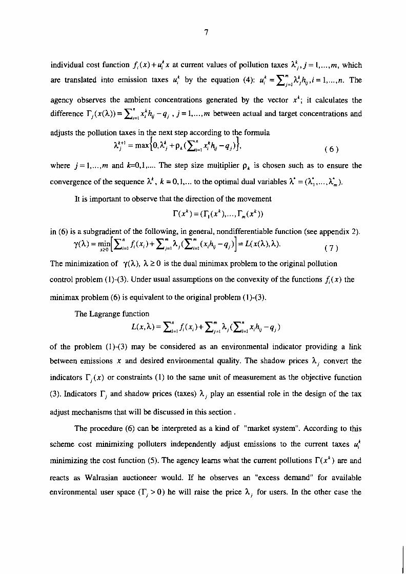
individual cost function f, (x) + ulk x at current values of pollution taxes q, j = 1,. . . ,m, which

are translated into emission taxes ulk by the equation (4): u,! = ELl h:h, ,i = 1, ... ,n. The

agency observes the ambient concentrations generated by the vector xk; it calculates the

difference r, (x(h)) = zn xlkh, - q, , j = I,. . . , m between actual and target concentrations and #=I

adjusts the pollution taxes in the next step according to the formula

= max{~ ,~ : + p k ( x n I=! x;hj -q,)},

where j = 1, ..., m and k=0,1, .... The step size multiplier p, is chosen such as to ensure the

convergence of the sequence hk , k = 0,1, ... to the optimal dual variables A* = (h; ,... , G). It is important to observe that the direction of the movement

r ( x k ) = ( r1(xk) ,..., rm(xk))

in (6) is a subgradient of the following, in general, nondifferentiable - function (see appendix 2).

The minimization of y(h), h 2 0 is the dual minimax problem to the original pollution

control problem (1)-(3). Under usual assumptions on the convexity of the functions f ; (x) the

minimax problem (6) is equivalent to the original problem (1)-(3).

The Lagrange function

of the problem (1)-(3) may be considered as an environmental indicator providing a link

between emissions x and desired environmental quality. The shadow prices h, convert the

indicators T,(x) or constraints (I) to the same unit of measurement as the objective function

(3). Indicators rj and shadow prices (taxes) A, play an essential role in the design of the tax

adjust mechanisms that will be discussed in this section .

The procedure (6) can be interpreted as a kind of "market system". According to this

scheme cost minimizing polluters independently adjust emissions to the current taxes ulk

minimizing the cost function (5). The agency learns what the current pollutions r ( x k ) are and

reacts as Walrasian auctioneer would. If he observes an "excess demand" for available

environmental user space ( r , > 0) he will raise the price h, for users. In the other case the

price will be lowered. Prices are a signal for users of environmental space to adjust their

emissions accordingly

The procedure (6) can be modified easily to include any additional a priori information

on possible tax values. For example, if we know an upper bound h,, j = 1, ..., rn on optimal

values q, the process (6) is modified as the following:

If the vector h* has to belong to a convex set A, the vector of new taxes hk" is calculated as

hk+' = Pr jA[hk + p k ~ ( h k ) ] , k = O,I, ... ( 9 )

wherePr j is the symbol of the projection operation on the set A :

Pr jA [y] = arg{minlly - hl12, h E A].

Examples of such operation on the set h 2 0 and on hypercube 0 5 h I h are given by

eqs. (6),(8). The main problem concerning the adjustment mechanisms (6), (8) and (9) is that

value pk , k = 0.1,. . . can not be chosen in order to decrease the total cost xn f, (xi ) by passing I='

from xk to xk" since this function is unknown to the agency. Besides this, the implementation

of a monotonic optimization procedure, which guarantees an improvement of the objective

function at each adjustment step, runs into difficulties since, in general, the direction of the

movement 1-(xk) in (6) is a subgradient of the non-differentiable function y(h) at h = hk . In

appendix 1 we outline the proof of the theorem showing that procedures (6). (8) and (9)

converge under rather general conditions for the values of the step size multipliers p,. Indeed

it may be any sequence po,pl. ... such that p, 20, xy=opk =m, for example pk = c / k , where

c is a positive constant. These conditions guarantee a convergence independently of the initial

vector of taxes hO. The procedure does not lead to monotonic improvements of total costs since

the choice of the step size multipliers p,, p, ,.. . is based on excess concentrations ( positive or

negative ) and not on the calculation of the total cost. Nevertheless the process enables to find

optimal taxes (see appendix 1). We also show that the convergence takes place even for

nonconvex functions f ' (x) , i = 1,. . . , n

4. Imperfect information of individual sources.

The deterministic pollution control problem discussed in section 3 assumed that the individual

sources have accurate information on costs. An implicit assumption in section 3 was that the

conditions determining costs remain unchanged during the whole period of adjusting the

environmental tax. Dynamic convergence to equilibrium (9) requires only the monitoring of

environmental indicators Tj (xk ) = xn x,! hi, - pj at emission levels xk = (x: ,...,xi), with 1=1

polluters minimizing costs f ; (x) + u:x at current emission charges u: = x;, k:.hi, .

In this section we drop the assumption of unchanged conditions. For each source the

costs of pollution control depend on a large number of factors. Some of them are of a rather

general kind, like weather conditions, prices of inputs; others are more specific; for example

types of fuel and other raw material used, type and age of existing pollution control equipment,

its state of maintenance, quality of operating personal, knowledge of available new abatement

technology. Even in such a case sources can not predict exact values of pollution control costs.

It will be assumed that the agency forms expectation about pollution control costs and sets out

to minimize the expected value of aggregate pollution control costs.

Actually the "state of the world" that affects cost will change during the adjustment

period. We assume that the polluter is informed about the current local conditions and

minimizes his costs given his certain information about factors affecting the cost-function. We

shall show that in the face of these assumptions the decentralized strategy of emission taxes

results in lower expected total pollution control costs than the centralized policy of setting

emission standards.

Suppose f, (xi ,v i ) is the cost function of the source i , where xi is an emission level

and v = (v, , ... , v, ) is a random vector representing variables that affect the source costs. It is

plausible to assume that under such circumstances the agency is able to compute only expected

costs (xi) = Ef; (xi, vi). We assume the existence of all necessary integrals. For example, we

can keep in mind the case that v has a finite number of values.

Let us first look at a policy of setting emission standards. The minimum cost emission

standard strategy for the environmental agency is found by solving the stochastic optimization

problem: minimize

subject to

z h l x i h G 59, . j = l , ..., rn, i = l , ..., n. (11 > If expected costs F; (x) = E i (x, V, ), i = 1,. . . ,n are convex functions, we can derive,

using duality theory, the existence of pollution charges 1; = (h; ,...,A:) and emission charges

u: = Em h;.hQ such that the least cost optimal strategy x: minimizes ]=I

for ui = u,', i = 1, ... ,m. Equation (12) represents the agency's expectation of the emission

reductions induced by charges u;. However, the agency's expectation of emissions will usually

not coincide with the actual reactions of polluters. Since each polluter i knows the situation

vi and costs at the source, he actually adjusts emission to the level xi (%, vi) minimizing

f;(x,vi)+uix, x 2 0 . ( 1 3 )

Therefore the environmental indicators r , (xk) of the procedure (6) are calculated at

random vector of emission levels xk = (x: ,..., xt ) minimizing cost functions (13) at random

situations v: , i = 1,. . . , n. In this case procedure (6) generates a sequence hO, h' , . . . of random

pollution charges and corresponding emission charges uO, u' , . . . . It can be shown (appendix 2)

that the direction of movement r ( x k ) = (TI (xk ), . . ., T, (xk )) in (6) is a stochastic subgradient of

the following function yl(h), which is similar to function y(h) defined by eq. (6):

In other words , the vector T(xk) is obtained formally by taking the gradient (with respect to

variables h = (h, ,..., h,) ) under the symbol of the mathematical expectation for observed

k k V, ,. ..,vf: and calculated x: ,..., x,. More precisely, it is possible to show (appendix 2) that the

random vector r ( x k ) is an unbiased estimate of a subgradient y i of function y' (h) at h = A! :

E[r(xk )lxk , hk ] = y: (hk ) , where E[. / .] is the conditional expectation symbol.

From the convergence of the stochastic quasigradient (see, for example, Ermoliev and

Wets (1987)) methods we can derive the convergence of the random sequence hO, A', . . . to the

minimal value of the function yl(h) , h 2 0 . The proof of this fact is close to the one given in

the appendix 1. Let us show that the expected cost of the emission charge strategy

u: = l i m x n h:.h, is less then the expected costs of the emission standard strategy derived it+- I='

from the problem (10)-(1 1).

It is easy to see that the minimization of y' (A) is a dual problem to the following: find

emission vector x(v) = (x, (v), ... , x,, (v)) that minimizes the expectation functional

subject to

x:=lExi(~)hij 5 q j , j = l , ..., m, xi(v)20. i = l , ..., n. ( 1 6 )

Suppose that x*(.) is an optimal solution of this problem. Consider the Lagrange

function

The existence of a saddle point (x* (v), A*) such that

L(x*(v), h) 5 L(x*(v),h*) 5 L(x(v),x) ( 17)

for all x(v) 2 0, h 2 0 follows from the convexity of the function i ( . ,v i ) for any fixed v .

Since decision x(-) in eqs. (15)-(16) depends on concrete situations v at sources, the optimal

value of the objective functions in eqs.(15)-(16) is smaller then the optimal value of the

objective function in eqs.(lO)-(1 1). Hence

F (x* ) 2 F (x* (.)) = ~ ( x * (v), X) = mar y ' (A).

5. Uncertainty on transfer coeflicients.

In the addition to the uncertainty involved in pollution control costs there exists

uncertainty about transfer coefficients. Transmission of pollutants by air is affected by factors

such as wind direction and speed and weather conditions. The concentration of effluents in

water depends on the volume and velocity of the flow. It is plausible to assume that the source

has better information on the specific conditions that determine the actual value of the transfer

coefficients than the agency has. Let us show that in such situations the policy of pollution

charges may be better than emission charges.

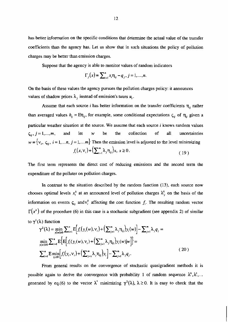
Suppose that the agency is able to monitor values of random indicators

r j ( ~ ) = z h 1 x i q U - q j , j= 1 ,.... n.

On the basis of these values the agency pursues the pollution charges policy: it announces

values of shadow prices h, instead of emission's taxes ui.

Assume that each source i has better information on the transfer coefficients q,, rather

than averaged values hU = Eq,,, for example, some conditional expectations G,, of q, given a

particular weather situation at the source. We assume that each source i knows random values

j 1 . m, and let w be the collection of all uncertainties

w = {v, , sU , i = I,. . . n, j = 1.. . . m) Then the emission level is adjusted to the level minimizing

The first term represents the direct cost of reducing emissions and the second term the

expenditure of the polluter on pollution charges.

In contrast to the situation described by the random function (13), each source now

chooses optimal levels x: at an announced level of pollution charges h: on the basis of the

information on events 5, and$ affecting the cost function 1. The resulting random vector

r ( x k ) of the procedure (6) in this case is a stochastic subgradient (see appendix 2) of similar

to y1 (A) function

y2(') = Y(W)M z := l~ [ f ; (~ i (w) ,v i )+ (z ; l h,~ij)y;(w)]-z;=, hjq, =

From general results on the convergence of stochastic quasigradient methods it is

possible again to derive the convergence with probability 1 of random sequence ho, h', ...

generated by eq.(6) to the vector h* minimizing y2(h), h 2 0. It is easy to check that the

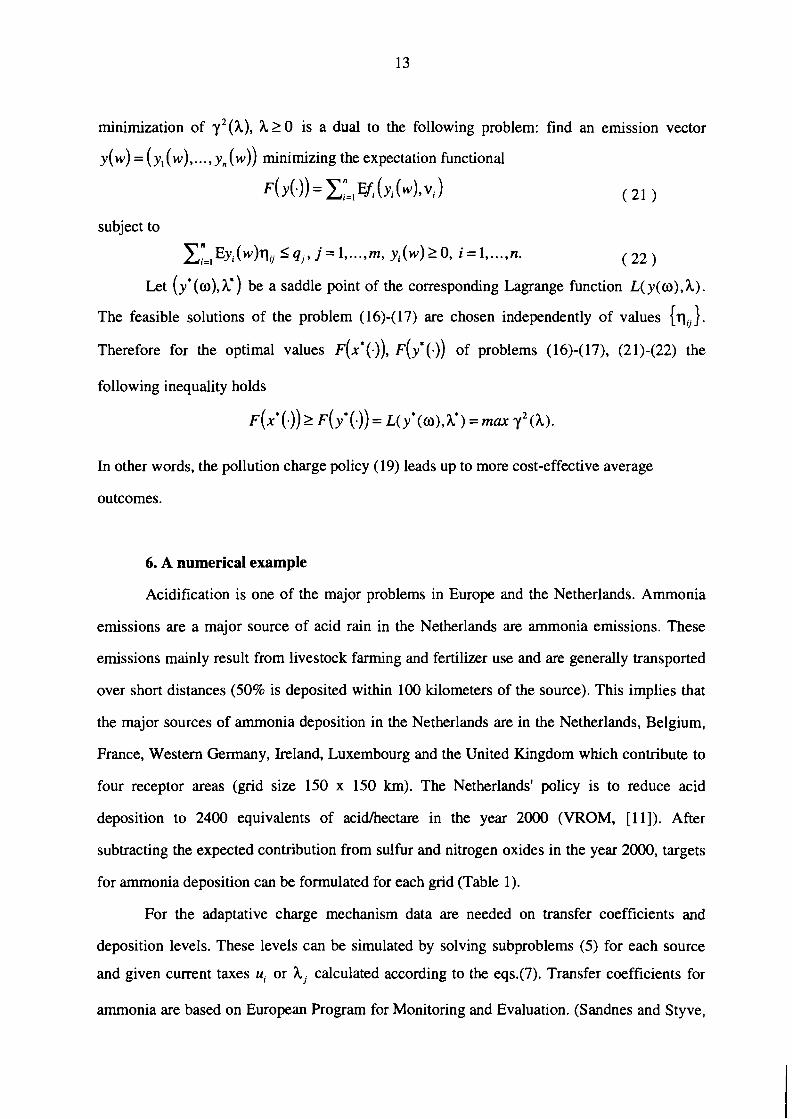
minimization of y2(h), h 2 0 is a dual to the following problem: find an emission vector

y (w) = ( y, ( w), . . . , y, (w)) minimizing the expectation functional

subject to

Let ( y* (a), h* ) be a saddle point of the corresponding Lagrange function L( y(a), A).

The feasible solutions of the problem (16)-(17) are chosen independently of values {q,,}.

Therefore for the optimal values ~ ( x * (a)), ~ ( y * ( a ) ) of problems (16)-(17), (2 1)-(22) the

following inequality holds

In other words, the pollution charge policy (19) leads up to more cost-effective average

outcomes.

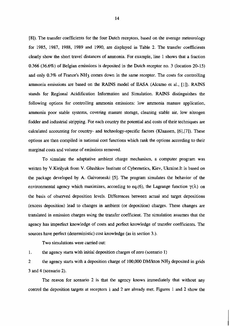
6. A numerical example

Acidification is one of the major problems in Europe and the Netherlands. Ammonia

emissions are a major source of acid rain in the Netherlands are ammonia emissions. These

emissions mainly result from livestock farming and fertilizer use and are generally transported

over short distances (50% is deposited within 100 kilometers of the source). This implies that

the major sources of ammonia deposition in the Netherlands are in the Netherlands, Belgium,

France, Western Germany, Ireland, Luxembourg and the United Kingdom which contribute to

four receptor areas (grid size 150 x 150 km). The Netherlands' policy is to reduce acid

deposition to 2400 equivalents of acidlhectare in the year 2000 (VROM, [Ill). After

subtracting the expected contribution from sulfur and nitrogen oxides in the year 2000, targets

for ammonia deposition can be formulated for each grid (Table 1).

For the adaptative charge mechanism data are needed on transfer coefficients and

deposition levels. These levels can be simulated by solving subproblems (5) for each source

and given current taxes u, or h, calculated according to the eqs.(7). Transfer coefficients for

ammonia are based on European Program for Monitoring and Evaluation. (Sandnes and Styve,

[8]). The transfer coefficients for the four Dutch receptors, based on the average meteorology

for 1985, 1987, 1988, 1989 and 1990, are displayed in Table 2. The transfer coefficients

clearly show the short travel distances of ammonia. For example, line 1 shows that a fraction

0.366 (36.6%) of Belgian emissions is deposited in the Dutch receptor no. 3 (location 20-15)

and only 0.3% of France's NH3 comes down in the same receptor. The costs for controlling

ammonia emissions are based on the RAINS model of IIASA (Alcamo et al., [I]). RAINS

stands for Regional Acidification Information and Simulation. RAINS distinguishes the

following options for controlling ammonia emissions: low ammonia manure application,

ammonia poor stable systems, covering manure storage, cleaning stable air, low nitrogen

fodder and industrial stripping. For each country the potential and costs of their techniques are

calculated accounting for country- and technology-specific factors (Klaassen, [6],[7]). These

options are then compiled in national cost functions which rank the options according to their

marginal costs and volume of emissions removed.

To simulate the adaptative ambient charge mechanism, a computer program was

written by V.Kirilyuk from V. Glushkov Institute of Cybernetics, Kiev, Ukraine.It is based on

the package developed by A. Gaivoronski [5]. The program simulates the behavior of the

environmental agency which maximizes, according to eq.(6), the Lagrange function y(h) on

the basis of observed deposition levels. Differences between actual and target depositions

(excess deposition) lead to changes in ambient (or deposition) charges. These changes are

translated in emission charges using the transfer coefficient. The simulation assumes that the

agency has imperfect knowledge of costs and perfect knowledge of transfer coefficients. The

sources have perfect (deterministic) cost knowledge (as in section 3.).

Two simulations were carried out:

1. the agency starts with initial deposition charges of zero (scenario 1)

2 the agency starts with a deposition charge of 100,000 DMkton NH3 deposited in grids

3 and 4 (scenario 2).

The reason for scenario 2 is that the agency knows immediately that without any

control the deposition targets at receptors 1 and 2 are already met. Figures 1 and 2 show the

values of both the total (annual) pollution control costs and the Lagrange function as a function

of the number of iterations. Figure 1 shows that after 12 iterations the total cost and Lagrange

function converges to around 2.9 billion DWyear (optimal value). Figure 2 clearly shows the

impact of starting from an initial deposition charge of 100,000 DMIkton NH3 deposited at

each receptor. In this case only seven iterations would be necessary to approach the cost-

minimum solution. Such an initial charge could be set if the environmental agency would ask

the individual source how they would respond to a certain emission charge before setting the

initial charges. If sources would overestimate their emission reductions in order to reduce the

charge level, the adaptation process would take longer and, as Figure 1 clearly indicates, costs

would be higher than necessary during the period of adaptation.

Figures 3 and 4 show the evolution of the emission charges over time for both

scenarios. Obviously, starting from a zero charge would initially lead (see step 2) very high

charges. This is especially so for Belgium and the Netherlands which have large impacts on the

deposition at the receptors located in the Netherlands. For Belgium the charges would reach

1596 x 1000 DWton NH3 at step 2 and would then gradually decrease to their final level of 72

x 1000 DWton ammonia controlled. Such overshooting might cause problems. Firstly, during

the adaptation period, charges and hence pollution control costs would be higher than

necessary. Secondly, if the fixed costs element of pollution control costs is high, high charges

may induce inflexibility since investments already taken are sunk costs. As Figure 5 shows,

starting from a deposition charge level of 100,000 DMkton NH3 deposited at receptors 3 and

4 would reduce the number of interactions to only seven. Moreover, the emission charges

would not fluctuate greatly over time. After some (small) overshooting at step 1 and

underscoring at step 2, the emission charges in all countries would gradually increase to the

level where the deposition constraints are met at minimum costs.

In conclusion, a system of adaptative deposition charges can be formulated that

converges to the cost-minimum solution even if the environmental agency has imperfect

knowledge on the costs. If some information on possible costs is available to the agency prior

to setting the initial charge, the adaptation can proceed faster and lead to less significant

fluctuations in costs and emission charge levels than if the agency starts with initial deposition

charges equal to zero.

7. Conclusions.

This paper discussed the feasibility of an emission charge policy applied to non

uniformly dispersed pollutants when the environmental authority's information on pollution

control costs and transfer coefficients is uncertain. We have shown that, contrary to established

opinion, the emission charge policy is both environmentally effective and cost effective. It has

also been demonstrated that under cost uncertainty deposition targets can be met but pollution

control cost will be lower if emission charges are imposed instead of emission standards. The

pollution charges are more cost effective than emission charges when the uncertainty is

involved in transfer coefficients.

It has been shown that an adjustment mechanism can be designed which resembles a

Walrasian process of "tatonnement". In a stepwise way taxes are adjusted such that ambient

concentration converges to the target levels and simultaneously total costs of pollution control

are minimized without the environmental agency having full information on costs andlor

transfer coefficients. In a mathematical sense the procedure deals with the solution of the

deterministic and stochastic minimax type problems. In the deterministic case this problem is

equivalent to the original pollution control problem assuming the cost functions are convex. In

general cases with stochastic costs and transfer coefficients the solution of the minimax

problems leads to more cost effective policies than the emission standard strategy. Since the

pollution control costs are unknown to the environmental authority the proposed adjustment

mechanisms are based on non-monotonic (deterministic and stochastic) techniques. By starting

from an arbitrary chosen vector of shadow prices, which are translated into emission taxes, the

authority observes the emission (or deposition) levels of polluters and assesses also the

environmental effectiveness of the solution by calculating the gaps between actual depositions

and deposition targets. When discrepancies are observed, shadow prices and corresponding

emission taxes are adjusted according to eq.(8) until all gaps are closed. The vector of

emissions then is both cost effective and environmentally effective.

Let us notice that this procedure can also be viewed as a "dialog" between the

environmental agency and polluters to investigate optimal taxes in order to avoid possible

troubles with investment in the case of overshooting taxes. The agency announces current

taxes and polluters report corresponding levels of emissions to the agency. The agency adjusts

taxes according to the proposed adjustment rule and announces new taxes and so on. Such a

preliminary, possibly highly computerized, dialog may provide a fairly accurate approximation

of taxes to be implemented in practice.

Our conclusion from the result is that there is no real difference in the applicability of

emission taxes, whether the environmental targets are formulated in terms of the emission goal

or as a set of ambient concentration standards. Under both types of environmental policy

emission charges can be applied as an instrument that is both cost and environmentally

effective and that is superior to an emission standard policy that could be environmentally

effective but less cost effective.

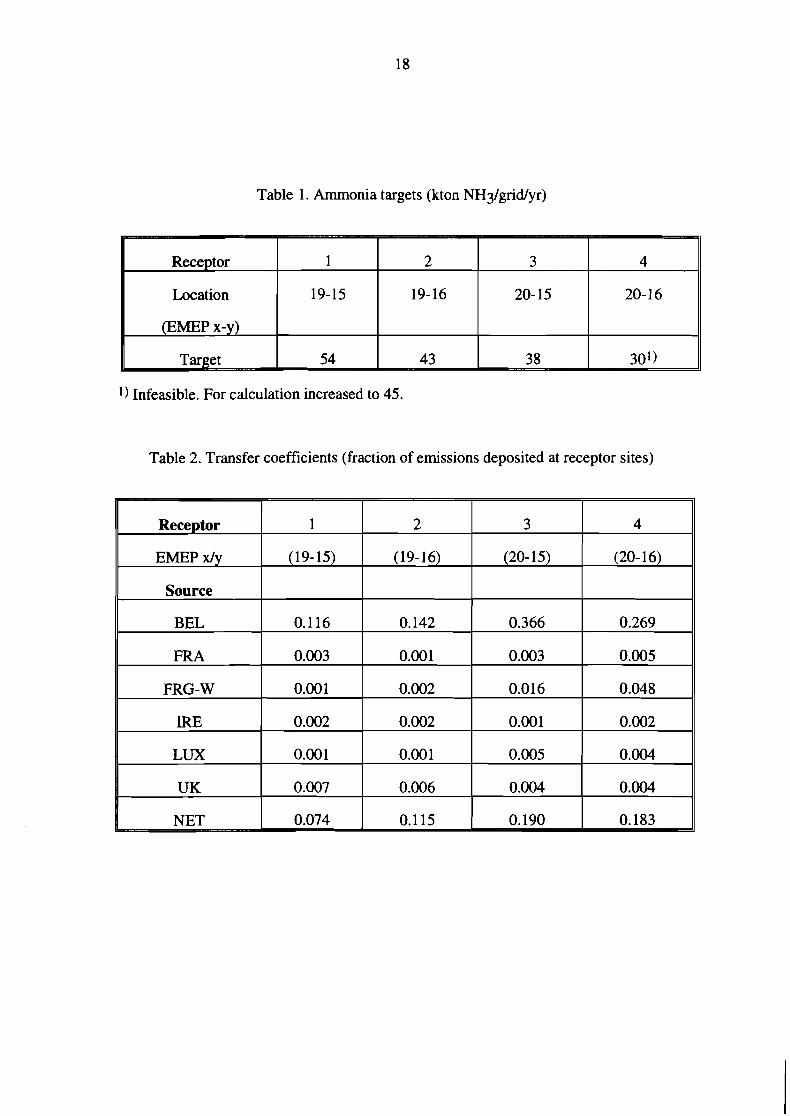
Table 1. Ammonia targets (kton NH3Igridlyr)

1) Infeasible. For calculation increased to 45.

Table 2. Transfer coefficients (fraction of emissions deposited at receptor sites)

Receptor

EMEP x/y

Source

BEL

1

(19-15)

0.1 16

2

(19-16)

0.142

3

(20- 1 5)

0.366

4

(20- 1 6)

0.269

Figure 1. Total costs and Lagrange function (106 DMIyr) with zero initial charges (scenario 1)

- Total costs . . @ . .

Lagrange function n

Figure 2. Total costs and Lagrange function (106 DMIyr) with zero initial charges (scenario 2)

Figure 3a. Emission charges (1000 DWton) with scenario (1) (iteration 1 - 5 )

BEL FRA FRG IRE LUX U K NET

Figure 3b. Emission charges (1000 DMJton) with scenario (1) (iteration 6 - 12)

r

BEL FRA FRG IRE LUX UK N ET

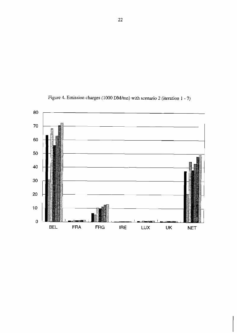
Figure 4. Emission charges (1000 DM/ton) with scenario 2 (iteration 1 - 7)

BEL FRA FRG IRE LUX UK NET

Appendix 1.

Asymptotic properties of the adjustment mechanisms.

Various requirements on the convergence of sequences hl, h2,. . . and xO, x1 , . . . generated

by rules (6),(8)-(9) can be derived from rather general results on the convergence of stochastic

quasigradient methods (see, for example, Ermoliev and Wets [4]). Let us outline the proof only

for the case where T(xk ) is the deterministic vector and the sequence p,, p,, ... satisfies the

condition

in particular, pk = c l k with c constant.

Suppose that p,, k = 0,1, ... satisfy conditions (23). We imply also the existence of

optimal solutions xO, x' , . . . defined according to eq.(S). Then the sequence of defined by the

rule (9), converges to the optimal dual variables (taxes) h* =(h;,...,h:). If in addition

xlk , k = 0, 1, . ..is the unique solution of the minimization problem (5) and f ; are convex

functions then the sequence xp , x,! , . . . converges to the cost effective emissions x,* , i = I,. . . , n.

Proof. From the projection operation definition follows that

where 11 - I denotes the Euclidean norm and (a,b) is the scalar product of vectors a and b. Since

r ( x k ) is a subgradient of the concave function y(h) at hk then for any vector h :

and hence

w h e r e y ( ~ ) = max y (h) .Therefore from the inequality (24) we have 120

From the problem formulation follows that x,(h) l x,(O) for each i=l, ... n and h 2 0.

Therefore, we can assume that IIr'(xk)l1 < const. In other words for some constant C

2 Define 6 , = Ilh* - hk 1 1 + C x W S= lr p: . From the above inequality follows that Sk+, 5 6,

and hence the sequence {6,} converges. Since zw L =O p i c - the sequence {llh* -hkl12} is also

convergent. From inequality (24) and taking into account that IIr(xk)ll c C (for some constant

C) we have

oiHh* - T I ~ ' - 2 x w k=O p k ( ~ ( ~ k ) , h * - h k ) + c z w k=o p i

Hence z- pk(r (xk) ,h* -hk) c -. Since x- pk = -, there exists a sequence {hki} such that k=O k=O

( r (xki ) ,h* -hkl) + 0 , I + -. Therefore y(hkl) + y(h*), I + -.

From this fact and the convergence of the sequence {~lh* -hkl12} follows the desired

result: hk + A*, k + DO.

Suppose 4 are convex functions. Consider now the sequence of emissions:

xk = urgmin L(x ,hk) , where L(x,h) is the Lagrange function of the pollution control 120

k problem. In other words, each component xjk of the vector xk = (x: , . . . , x,, ) is the solution of

the subproblem (5) for h, = h:, j = 1, ... ,m. Let us show that xk + x*, k + - From the definition of y(h) we have L(xk ,hk )= y (hk) . From the convergence

hk +A*, k + - and the inequality (25) follows that y(hk)+ y(h*). Therefore from the

duality theory follows that

L(xk ,Ak) = y (hk ) + y(h*) = L(x*,h*).

Suppose that xk does not converge to x*, that is to say there exists a sequence

xki + E f x*. hen

L(xki , hki ) = argmin ~ ( x , hki ) + L(Y, A*) 120

Since x* = urgmin L(x , h*) is uniquely defined, Y = x*. The contradiction completes the proof. xZO

Appendix 2. On the calculation of stochastic subgradients.

Functions y (h ) , y l (h ) , y 2 ( h ) belong to the following family of functions. Suppose

cp(x, h ,0) is a function defined on x E Rn , h E Rn and 0 E 0, where (0,3, P ) is a probability

space. Assume that (p(x,.,8) is a concave continuously differentiable function, cp , is its

gradient and there exist all necessary integrals which are considered further.

Consider maximization of the function

g(h) = E min ~[cp(x , A, e)lA] = ~rp(x (h , w), h , 8 )

where E[cp1A] is the conditional expectation with respect to a given family of events

o E A c 9. Let us show that the vector

5 = c p i (x. h,e)l x=x,A,wl

is an unbiased estimate of a subgradient g, (stochastic subgradient of g,):

g ( p ) - g(h) 5 (E[%lh],p - A ) 9 w. Indeed from the concavity of cp(x,., 8 ) follows

E[cp(x(p, w), p, e)lA] - ~[cp(x(h , w), h,e)lA] 5

E [ v ( x ( ~ , w)p, ~ ) I A ] - E [ v ( x ( ~ , w), h , e~A)] 5 (E[cp,(h, w), A, el A], p -A) .

The desired result follows now by taking the conditional expectation (for fixed p, h ) in both

sides of this inequality: g ( p ) - g(h) 5 (~ip, (x (h , w), h , 8), p - h) .

References

1 . J. Alcamo, R. Shaw and L. Hordijk (eds.) 1990 The RAINS model of acidijkation, science

and strategies in Europe. Kluwer Academic Publishers, Dordrecht/Boston/London . 2. W. Baumol and W.Oates 1971 The use of standards and prices for protection of the

environment. The Swedish Journal of Economics, 73 (March 1971), pp.42-54.

3. P. Bohm and C.S.Russe1 1985 Comparative analysis of alternative policy instruments. In:

A. V. Kneese and J.L.Sweeney (Eds) Handbook of natural resource and energy economics. Vol.

I, pp. 395-460. Amsterdam, New York, Ogord: North-Holland.

4. Y. Ennoliev and R. Wets (Eds.) 1988 Numerical techniques for Stochastic Optimization.

Springer - Verlag, Computational Mathematics.

5. A. Gaivoronski 1988 Implementation of Stochastic Quasigradient Methods, In: Y. Ermoliev

and R. Wets (Eds.) Numerical techniques for Stochastic Optimization. Springer - Verlag,

Computational Mathematics.

6. G. Kluassen 1991 Costs of controlling ammonia emissions in Europe. Status Report SR-91-

03. IIASA, Laxenburg, Austria.

7. G. Klaassen 1994 Cforthcoming) Options and costs of controlling ammonia emissions in

Europe. European Review of Agricultural Economics.

8. H. Sandnes and H. Styve 1992 Calculated budgets for airborne acidifying components in

Europe, 1985, 1987, 1988, 1989, 1990 and 1991. EMEP/SC- W report 1/92. Meteorological

Synthesizing Center- West, the Norwegian Meteorological Institute, Oslo, Norway.

9. T.H. Tietenberg 1974 Derived decision rules for pollution control in a general equilibrium

space economy, J.Environ: Econ. Manag. 1, 1-16.

10. T.H. Tietenberg 1978 Spatially diterentiated air pollutant emission charges: an economic

and legal analysis. The American Economic Review Land Economics V54, pp.265-277

1 1 . VROM 1989 National Environmental Policy Plan Plus. Ministry of Housing, Physical

Planning and Environment, The Hague, The Netherlands.