Embed Size (px)
Citation preview

seismic wave propagation through spherical sections
including anisotropy and visco-elastic dissipation
3D heterogeneities of all Earth model properties
inversion of seismic observables for 3D Earth structure


data
synthetic
period: 5 s
modelling volcanic
earthquakes on Iceland
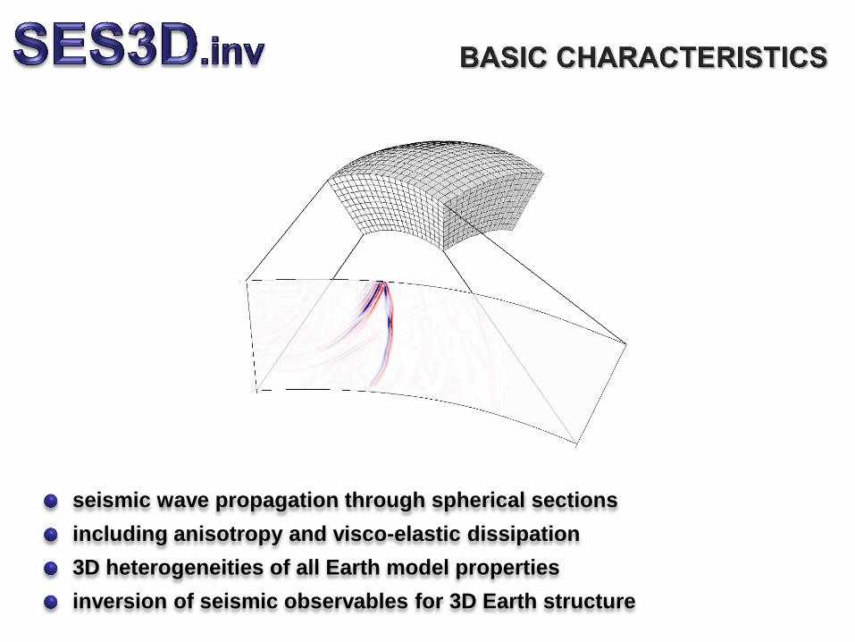
A collection of recent applications
sensitivity analysis:
How is my observable affected
by Earth structure? 15 s P wave
50 s Rayleigh wave
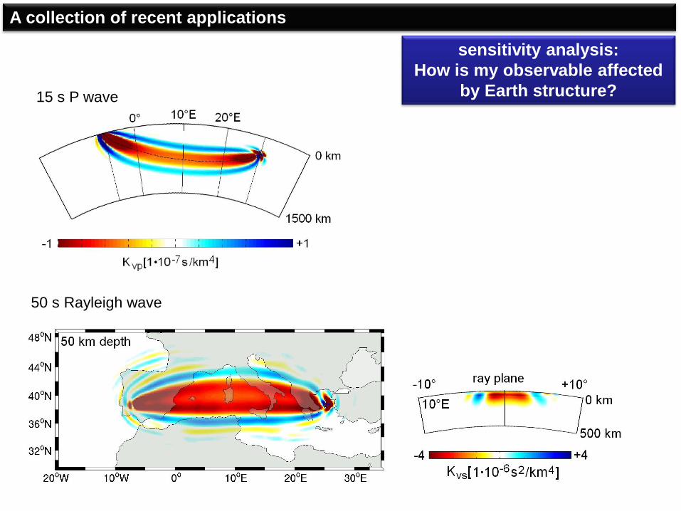
A collection of recent applications
A collection of recent applications
sensitivity analysis:
How is my observable affected
by Earth structure?
by Denise de Vos
Cross-correlation
measurements for regional
scale tomography.
Validation of the 2-station
method.
source
receiver 1
receiver 2

A collection of recent applications
sensitivity analysis:
How is my observable affected
by Earth structure?
||||
||||
rotation
velocityvelocitySapparent
by Moritz Bernauer
amplitudewaveS
source
source
receiver
receiver

waveform inversion for 3D
Earth structure
data initial model final model
T = 30 s
A collection of recent applications

Tomography is a 3-stage process:
(1) forward problem
(2) sensitivities
(3) optimisation
A collection of recent applications
waveform inversion for 3D
Earth structure
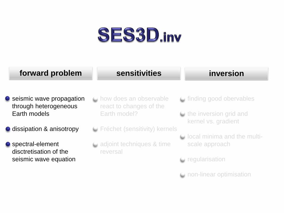
forward problem sensitivities inversion
seismic wave propagation
through heterogeneous
Earth models
dissipation & anisotropy
spectral-element
disctretisation of the
seismic wave equation
how does an observable
react to changes of the
Earth model?
Fréchet (sensitivity) kernels
adjoint techniques & time
reversal
finding good obervables
the inversion grid and
kernel vs. gradient
local minima and the multi-
scale approach
regularisation
non-linear optimisation

forward problem sensitivities inversion
finding good obervables
the inversion grid and
kernel vs. gradient
local minima and the multi-
scale approach
regularisation
non-linear optimisation
seismic wave propagation
through heterogeneous
Earth models
dissipation & anisotropy
spectral-element
disctretisation of the
seismic wave equation
how does an observable
react to changes of the
Earth model?
Fréchet (sensitivity) kernels
adjoint techniques & time
reversal
Thursday morning Thursday afternoon Friday morning

PART I
NUMERICAL SOLUTION OF THE SEISMIC WAVE EQUATION
1. Introduction
2. Spectral-element discretisation
3. Practical
4. Special topics (dissipation, point sources, absorbing boundaries)

Introduction

Introduction
(x,t)f(x,t)u(x,t)C(x,t)uρ ilkijklji ][
elastic displacement field
density elastic tensor external forces

Introduction
(x,t)f(x,t)u(x,t)C(x,t)uρ ilkijklji ][
elastic displacement field
density elastic tensor external forces
spectral-elements in a spherical section
operates in natural spherical coordinates
visco-elastic dissipation
radial anisotropy
absorbing boundaries: PML
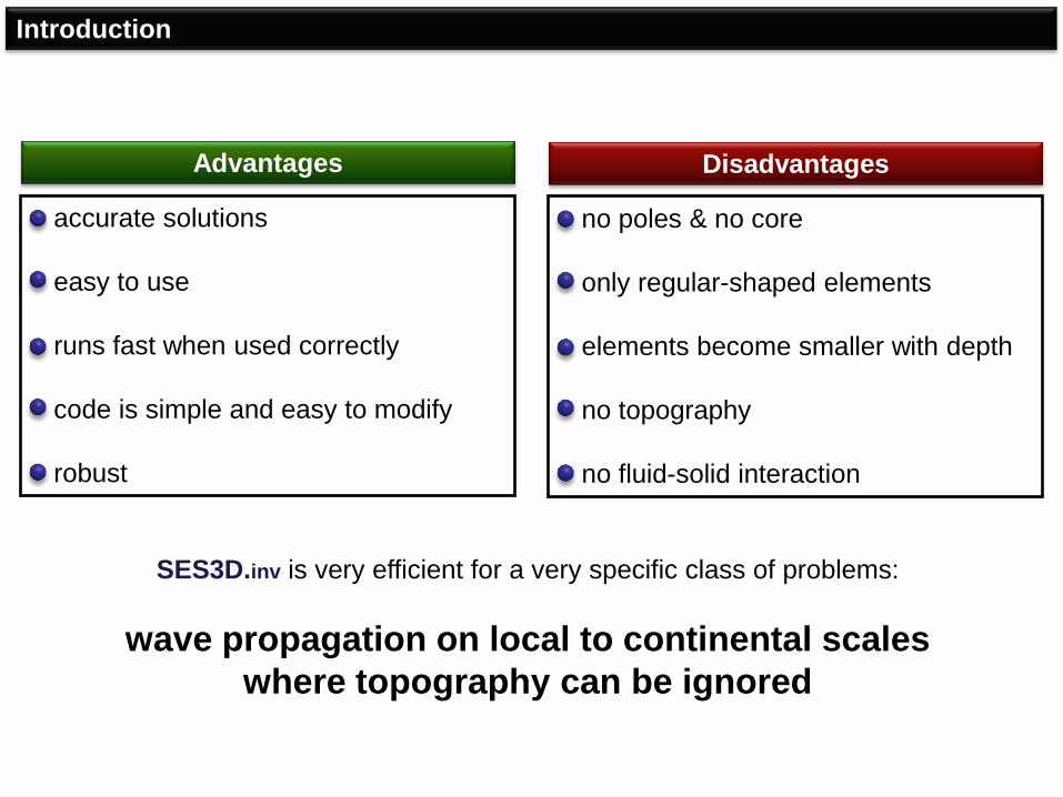
Introduction
accurate solutions
easy to use
runs fast when used correctly
code is simple and easy to modify
robust
Advantages
no poles & no core
only regular-shaped elements
elements become smaller with depth
no topography
no fluid-solid interaction
Disadvantages
SES3D.inv is very efficient for a very specific class of problems:
wave propagation on local to continental scales
where topography can be ignored

Spectral-element discretisation

Spectral-element discretisation
Priolo, Carcione & Seriani: 1994
reflection and transmission of
surface waves at material
discontinuities
• originally developed in fluid dynamics (Patera, 1984)
• migrated to seismology in the early 1990‘s (Seriani & Priolo, 1991)
• major advantage: accurate modelling of interfaces and the free surface (with topography)
The SEM origins

Spectral-element discretisation
The SEM concept in 1D: Weak form of the wave equation
0L)u(t,u(t,0)
xx
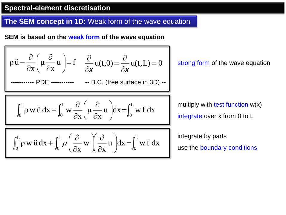
SEM is based on the weak form of the wave equation
0 L
vibrating string of length L
fux
μx
uρ
strong form of the wave equation
----------- PDE ----------- -- B.C. (free surface in 3D) --

Spectral-element discretisation
The SEM concept in 1D: Weak form of the wave equation
0L)u(t,u(t,0)
xx
SEM is based on the weak form of the wave equation
fux
μx
uρ
strong form of the wave equation
----------- PDE ----------- -- B.C. (free surface in 3D) --
multiply with test function w(x)
integrate over x from 0 to L
L
0
L
0
L
0dxfwdxu
xμ
xwdxuwρ
L
0
L
0
L
0dxfwdxu
xw
xdxuwρ
integrate by parts
use the boundary conditions

Spectral-element discretisation
L
0
L
0
L
0dxfwdxu
xw
xdxuwρ
Solving the weak form of the wave equation means
to find a displacement field u(x,t) such that
is satisfied for any differentiable test function w(x).
The SEM concept in 1D: Weak form of the wave equation

Spectral-element discretisation
L
0
L
0
L
0dxfwdxu
xw
xdxuwρ
Solving the weak form of the wave equation means
to find a displacement field u(x,t) such that
is satisfied for any differentiable test function w(x).
The SEM concept in 1D: Weak form of the wave equation
Basis of element-based methods (e.g. finite elements, spectral elements,
discontinuous Galerkin)
Boundary conditions are implicitly satisfied (no additional work required, as
in finite-difference methods)
Spectral-element discretisation
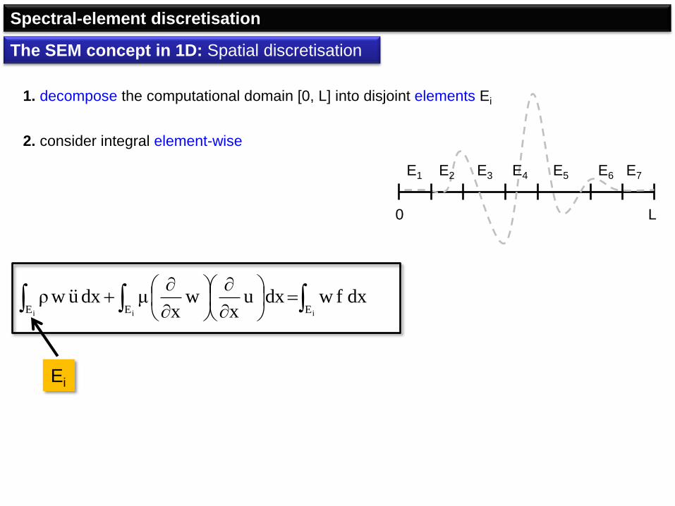
The SEM concept in 1D: Spatial discretisation
iii EEEdxfwdxu
xw
xμdxuwρ
0 L
E1 E2 E3 E4 E5 E6 E7
1. decompose the computational domain [0, L] into disjoint elements Ei
2. consider integral element-wise
Ei

Spectral-element discretisation
The SEM concept in 1D: Spatial discretisation
iii EEEdxfwdxu
xw
xμdxuwρ
0 L
E1 E2 E3 E4 E5 E6 E7
Ei
3. map each element to the reference interval [-1, 1]
x
Ei
-1 1 y
y = Fi(x)

Spectral-element discretisation
The SEM concept in 1D: Spatial discretisation
iii EEEdxfwdxu
xw
xμdxuwρ
0 L
E1 E2 E3 E4 E5 E6 E7
Ei
x
Ei
-1 1 y
y = Fi(x)
Is the same for every element !!!
All elements can now be treated in the same way.
...dydy
dxuwρ
1
1-
Spectral-element discretisation
The SEM concept in 1D: Spatial discretisation
...dydy
dxuwρ
1
1-
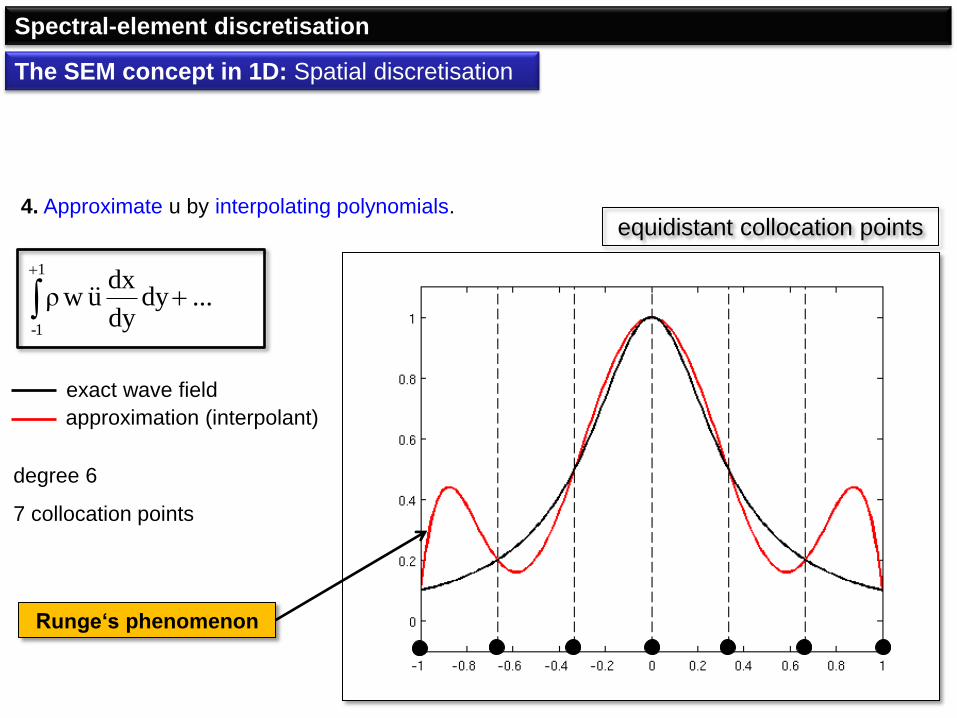
4. Approximate u by interpolating polynomials. equidistant collocation points
exact wave field
approximation (interpolant)
degree 6
7 collocation points
Runge‘s phenomenon

Spectral-element discretisation
The SEM concept in 1D: Spatial discretisation
...dydy
dxuwρ
1
1-
4. Approximate u by interpolating polynomials.
Gauss-Lobatto-Legendre points
exact wave field
approximation (interpolant)
degree 6
7 collocation points
Spectral-element discretisation
The SEM concept in 1D: Spatial discretisation
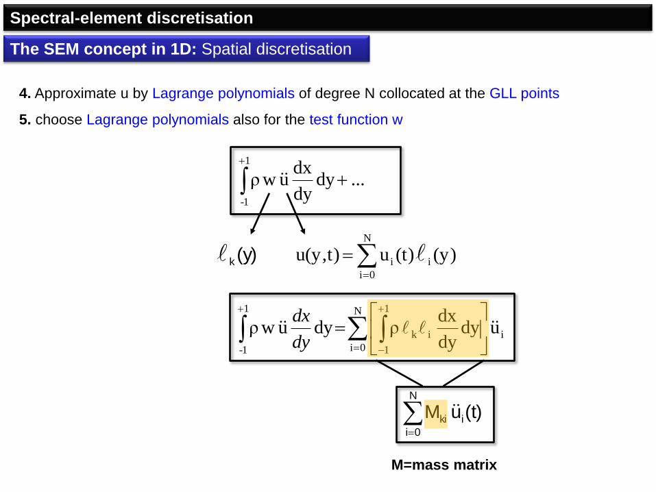
4. Approximate u by Lagrange polynomials of degree N collocated at the GLL points
5. choose Lagrange polynomials also for the test function w
N
0i
ii (y)(t)ut)u(y, (y)k
...dydy
dxuwρ
1
1-
N
0i
i
1
1
ik
1
1-
udydy
dx ρdyuwρ
dy
dx
N
0i
iki (t)uM
M=mass matrix
Spectral-element discretisation
The SEM concept in 1D: Spatial discretisation
N
0i
i
1
1
ik
1
1-
udydy
dx ρdyuwρ
dy
dx
N
0i
iki (t)uM
M=mass matrix
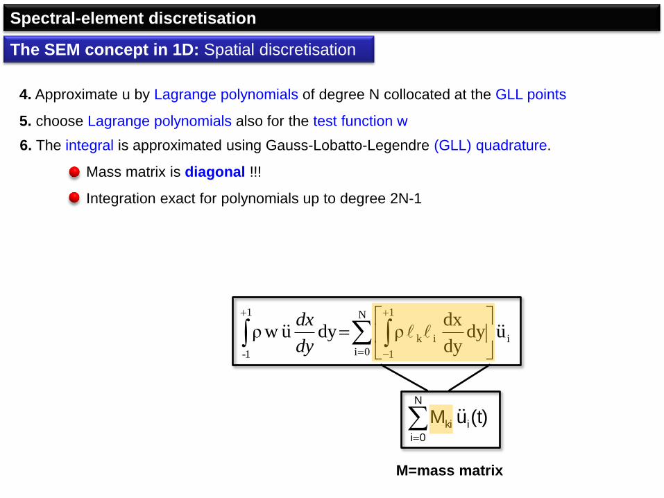
6. The integral is approximated using Gauss-Lobatto-Legendre (GLL) quadrature.
Mass matrix is diagonal !!!
Integration exact for polynomials up to degree 2N-1
4. Approximate u by Lagrange polynomials of degree N collocated at the GLL points
5. choose Lagrange polynomials also for the test function w
Spectral-element discretisation
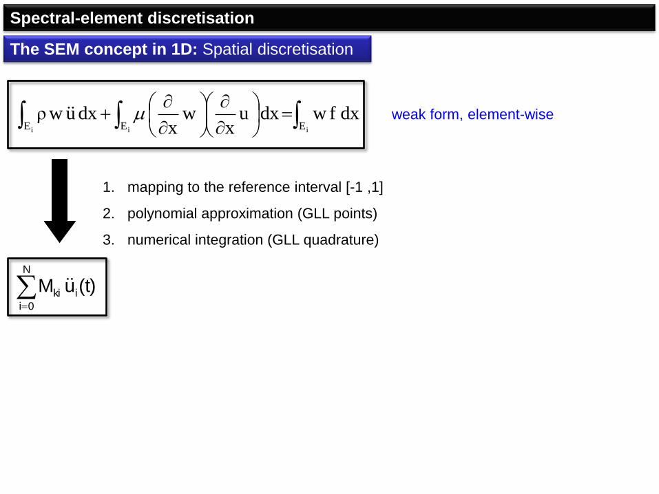
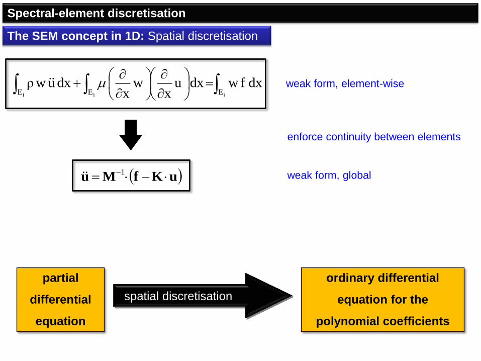
iii EEEdxfwdxu
xw
xdxuwρ weak form, element-wise
1. mapping to the reference interval [-1 ,1]
2. polynomial approximation (GLL points)
3. numerical integration (GLL quadrature)
N
0i
iki (t)uM
The SEM concept in 1D: Spatial discretisation

Spectral-element discretisation
iii EEEdxfwdxu
xw
xdxuwρ weak form, element-wise
The SEM concept in 1D: Spatial discretisation
repeat this for the remaining two terms …
N
0i
iiki
N
0i
iki fuK(t)uM
stiffness matrix discrete force vector
Spectral-element discretisation
iii EEEdxfwdxu
xw
xdxuwρ weak form, element-wise
The SEM concept in 1D: Spatial discretisation
uKfMu 1
partial
differential
equation
spatial discretisation
ordinary differential
equation for the
polynomial coefficients
enforce continuity between elements
weak form, global
Spectral-element discretisation
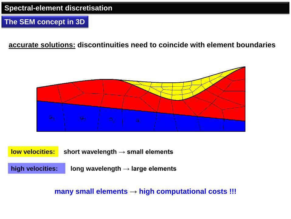
The SEM concept in 3D
accurate solutions: discontinuities need to coincide with element boundaries
low velocities: short wavelength → small elements
high velocities: long wavelength → large elements
many small elements → high computational costs !!!

Spectral-element discretisation
The SEM concept in 3D
Realistic example: The Grenoble valley
Stupazzini et al. (2009)

Spectral-element discretisation
The SEM concept in 3D
Essentially the same as in 1D:
1. mapping to the reference cube [-1 ,1]3
2. polynomial approximation (GLL points)
3. numerical integration (GLL quadrature)
uKfMu 1
if
lu
kxijkl
C
jxi
uρ
deformed element reference cube

Spectral-element discretisation
The SEM concept in 3D: SES3D discretisation
Each element is a small spherical subsection.
Discretisation of a spherical section without poles and core.
Speeds up the calculations.
Simplifies the programme code.
Reduces flexibility.

Practical
1. SES3D file structure
2. Input files
3. Model generation
4. Forward simulation: wiggly lines – at last!
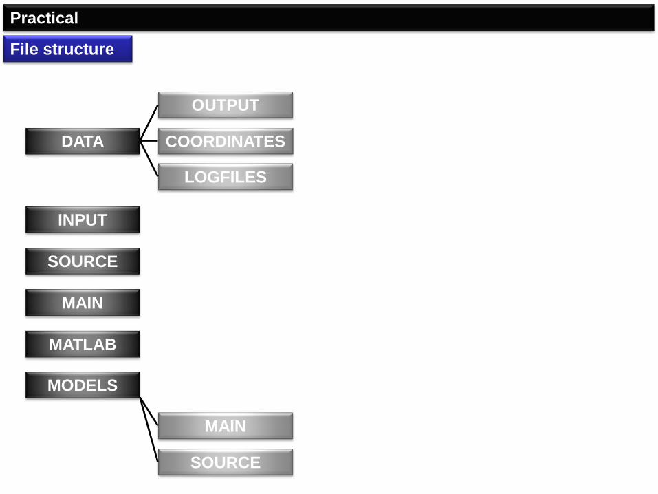
Practical
File structure
SOURCE
DATA
MAIN
MODELS
MATLAB
INPUT
OUTPUT
COORDINATES
LOGFILES
MAIN
SOURCE

Practical
File structure
SOURCE
DATA
MAIN
MODELS
MATLAB
INPUT
OUTPUT
COORDINATES
LOGFILES
MAIN
SOURCE
seismograms, snapshots, kernels
files with collocation point coordinates
logfiles written during runtime
simulation parameters, source time function, receivers
FORTRAN source code
executables and scripts for parallel jobs
collection of Matlab (plotting) tools
Earth model properties (density, elastic parameters, …)
executables for model generation
source code for model generation

Practical
Example
regional-scale wave
propagation
1 processor (not parallel)

Practical
Input files: Par file
total number of time steps (nt=500)
time increment in seconds (dt=0.75)
simulation length = nt∙dt (= 375 s)
dt must satisfy the stability criterion:
3.0,max
min cv
dxcdt

Practical
source position
colatitude (90°-latitude) in ° (90°)
longitude in ° (2.5°)
depth in m, not km (30000 m)
Input files: Par file

Practical
source characteristics
source type: 1,2,3=single forces, 10=moment tensor
moment tensor components in Nm
Mtt, Mpp, Mrr, Mtp, Mtr, Mpr
Input files: Par file
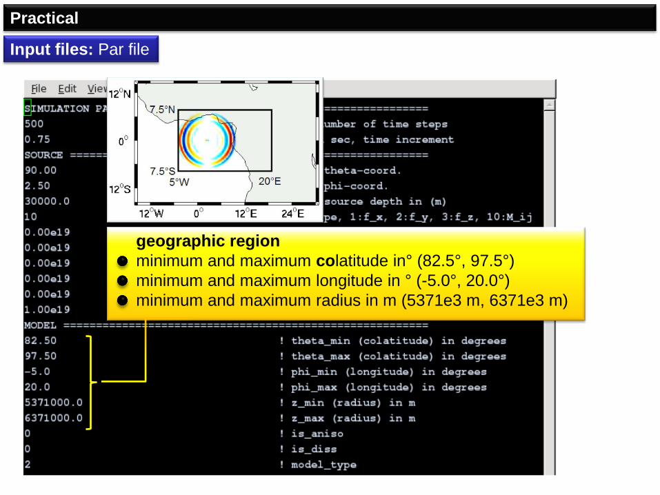
Practical
geographic region
minimum and maximum colatitude in° (82.5°, 97.5°)
minimum and maximum longitude in ° (-5.0°, 20.0°)
minimum and maximum radius in m (5371e3 m, 6371e3 m)
Input files: Par file

Practical
Input files: Par file
radial anisotropy switched on (=1) or off (=0)
visco-elastic dissipation switched on (=1) or off (=1)
structural model (2=PREM)
Practical
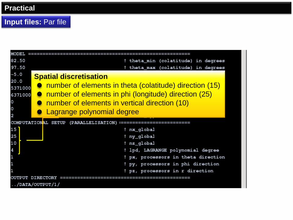
Input files: Par file
Spatial discretisation
number of elements in theta (colatitude) direction (15)
number of elements in phi (longitude) direction (25)
number of elements in vertical direction (10)
Lagrange polynomial degree
Practical
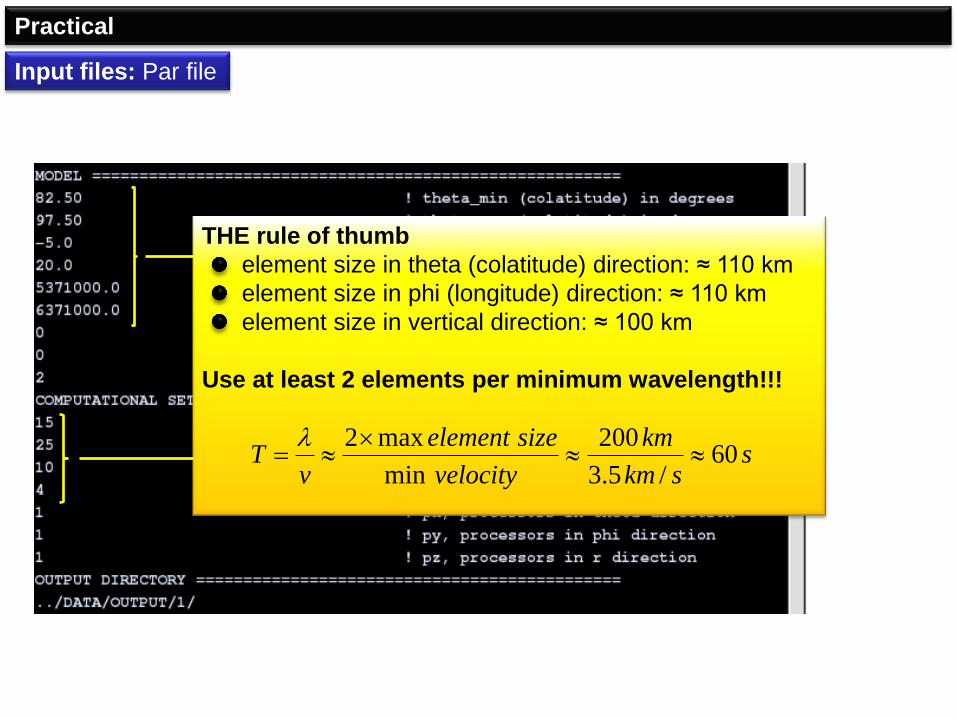
Input files: Par file
THE rule of thumb
element size in theta (colatitude) direction: ≈ 110 km
element size in phi (longitude) direction: ≈ 110 km
element size in vertical direction: ≈ 100 km
Use at least 2 elements per minimum wavelength!!!
sskm
km
velocity
sizeelement
vT 60
/5.3
200
min
max2
Practical
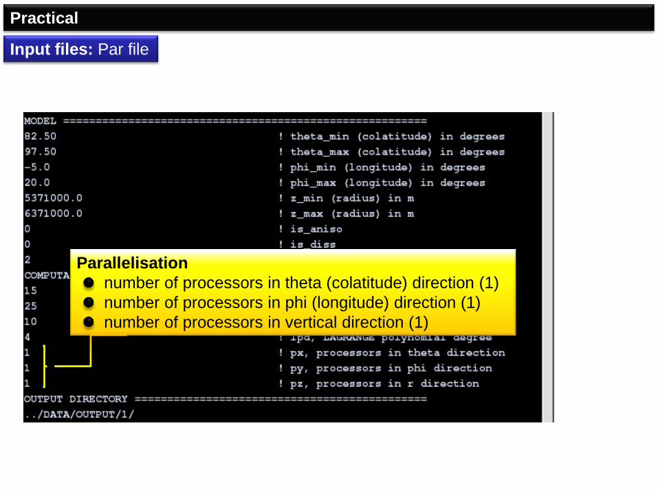
Input files: Par file
Parallelisation
number of processors in theta (colatitude) direction (1)
number of processors in phi (longitude) direction (1)
number of processors in vertical direction (1)
Practical
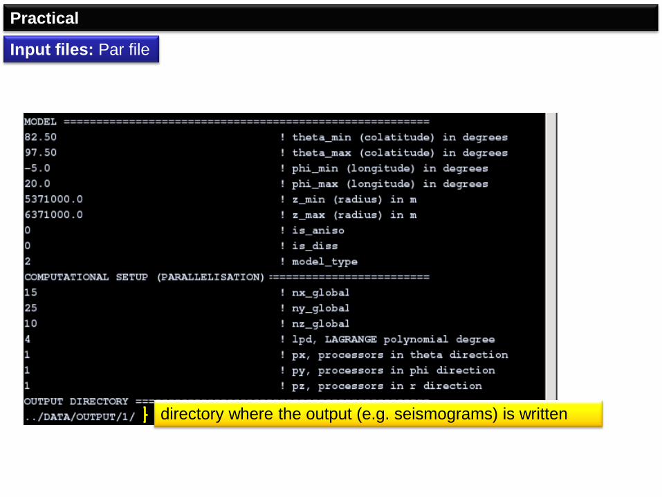
Input files: Par file
directory where the output (e.g. seismograms) is written

Practical
Input files: Par file
write snapshots of the wave field (1=yes, 0=no) into the
OUTPUT DIRECTORY every ssamp (=100) time steps
Practical
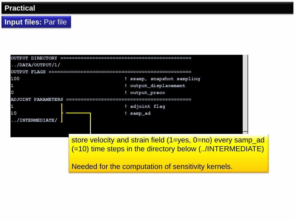
Input files: Par file
store velocity and strain field (1=yes, 0=no) every samp_ad
(=10) time steps in the directory below (../INTERMEDIATE)
Needed for the computation of sensitivity kernels.
Practical
Input files: source time function (stf)
Heaviside function, bandpass-filtered between 60 s and 500 s
lower cutoff period (60 s) dictated by the size of the elements
upper cutoff (500 s) ensures that the stf returns to zero
always use bandlimited stf‘s
time domain freq. domain
Practical
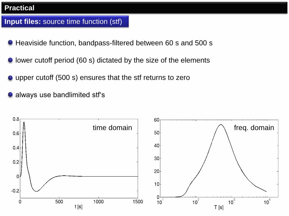
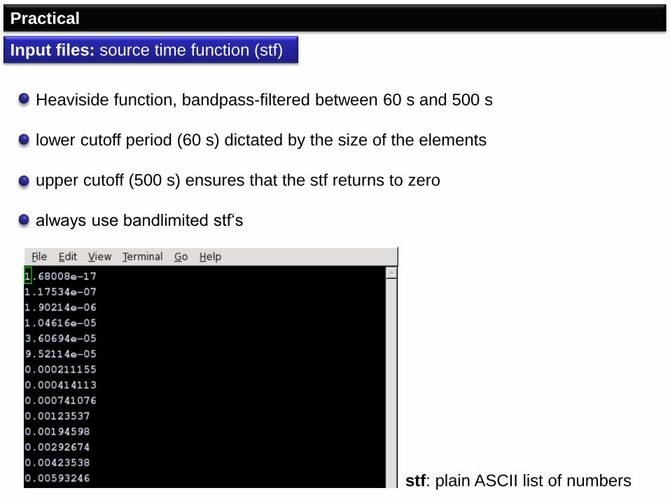
Input files: source time function (stf)
Heaviside function, bandpass-filtered between 60 s and 500 s
lower cutoff period (60 s) dictated by the size of the elements
upper cutoff (500 s) ensures that the stf returns to zero
always use bandlimited stf‘s
stf: plain ASCII list of numbers

Practical
Input files: receiver configuration (recfile)
number of receivers (2)
first station name (XX01)
station colatitude (90.0°), longitude (7.5°), depth (0.0 m)
second station name (XX02)
…

Practical
Model generation
MODELS
MAIN
SOURCE
run generate_models.exe
1 file for each model parameter (lambda, mu, 1/rho) …
… and for each processor.
Practical
Run SES3D
MAIN run main.exe and wait …

Practical
Simulation
75 s

Practical
Simulation
150 s
Practical
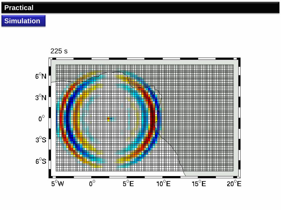
Simulation
225 s
Practical
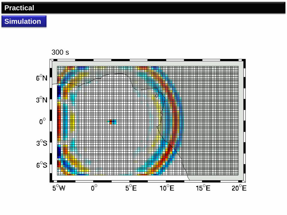
Simulation
300 s

Practical
Simulation
375 s
km/s4.1s75
km305
s75
elements2v 4
3
fundamental-mode Rayleigh wave @ 60 s period

Practical
Results: Synthetic seismograms
vr [m/s]
vϕ [m/s]
vθ [m/s]
prominent Rayleigh wave
no displacement on the N-S
component
pollution by reflections
because absorbing
boundaries are switched off

Special Topics
1. Visco-elastic dissipation
2. Point sources
3. Absorbing boundaries

Special Topics
Dissipation
Again, the concept in 1D:
The Earth is assumed to have a visco-elastic rheology defined as:
This convolution is very inconvenient in time-domain wave propagation!

Special Topics
Dissipation
Again, the concept in 1D:
The Earth is assumed to have a visco-elastic rheology defined as:
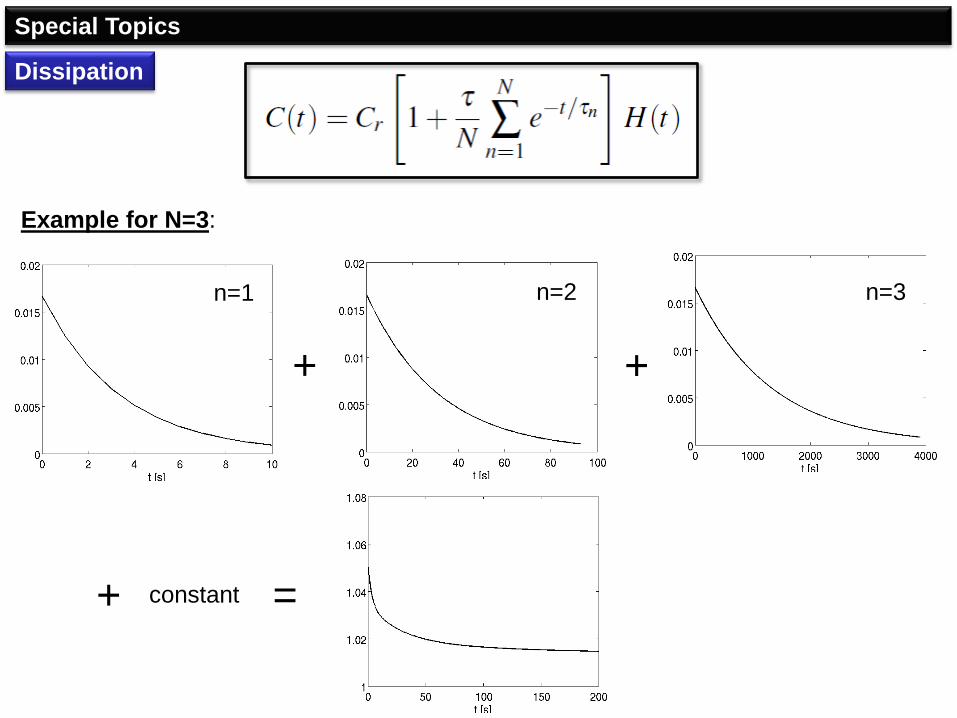
For the stress-relaxation function C(t) one assumes a superposition of standard-
linear solids:
C(t) describes the stress that occurs in response to a unit step strain.
The parameters of C(t) are chosen such that the corresponding Q(ω)
takes a specific form.
Special Topics
Dissipation
+ +
+ = constant
Example for N=3:
n=1 n=2 n=3
Special Topics
Dissipation
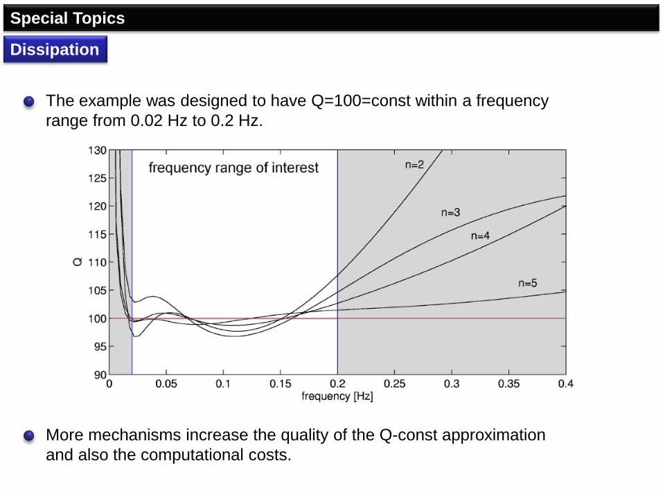
The example was designed to have Q=100=const within a frequency
range from 0.02 Hz to 0.2 Hz.
More mechanisms increase the quality of the Q-const approximation
and also the computational costs.

Special Topics
Point sources
There are generally two ways of implementing a point source – each with its
advantages and disadvantages:

Special Topics
Point sources
There are generally two ways of implementing a point source – each with its
advantages and disadvantages:
1. Grid point implementation
Force acts at the grid point that is closest to the true point source location.
grid points
implemented
point source
true point
source location
easy to implement
correct near field
numerical error when the true
location of the point force is too
far from the nearest grid point
Special Topics
Point sources
There are generally two ways of implementing a point source – each with its
advantages and disadvantages:
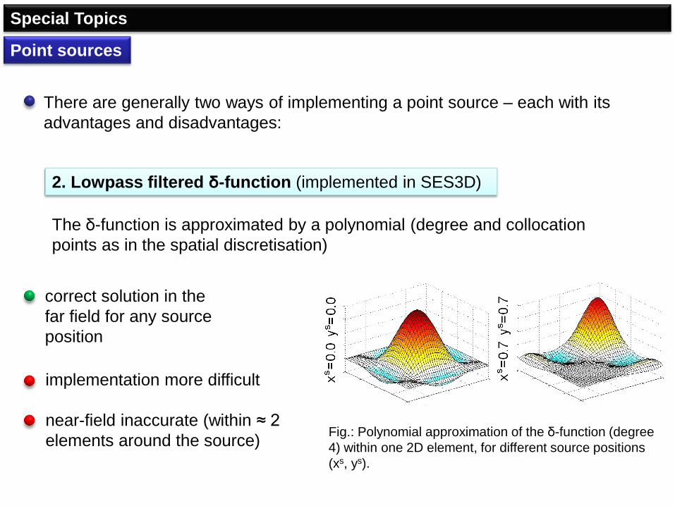
2. Lowpass filtered δ-function (implemented in SES3D)
The δ-function is approximated by a polynomial (degree and collocation
points as in the spatial discretisation)
correct solution in the
far field for any source
position
implementation more difficult
near-field inaccurate (within ≈ 2
elements around the source) Fig.: Polynomial approximation of the δ-function (degree
4) within one 2D element, for different source positions
(xs, ys).

Special Topics
Absorbing boundaries
Methods to avoid reflections from unphysical boundaries fall into 2 categories:
1. Absorbing boundary conditions
Boundary conditions that prevent the popagation of energy into the medium.
easy and elegant implementation
highly inefficient for large angles of incidence
2. Absorbing boundary layers (implemented in SES3D)
Boundary layers where the amplitudes of incoming waves decay rapidly
efficient for all angles of incidence
implementation more involved
can be unstable
can be unstable

Special Topics
Absorbing boundaries
2. Absorbing boundary layers (implemented in SES3D)
Perfectly Matched Layers (PML) are the most popular and efficient
absorbing technique.
Wave equation is modified within the boundary region so that incoming
waves decay exponentially:
Fig.: SES3D wavefield snapshots, illustrating the absorption of energy within the PML region.

Special Topics
Absorbing boundaries
2. Absorbing boundary layers (implemented in SES3D)
Perfectly Matched Layers (PML) are the most popular and efficient
absorbing technique.
Wave equation is modified within the boundary region so that incoming
waves decay exponentially:
Fig.: Total kinetic energy within the
model as a function of time. The
energy decreases rapidly but does
not reach 0 due to imprefect
absorption.