Embed Size (px)
Citation preview
Ocean Sci., 8, 567–586, 2012www.ocean-sci.net/8/567/2012/doi:10.5194/os-8-567-2012© Author(s) 2012. CC Attribution 3.0 License.
Ocean Science
In situ determination of the remote sensing reflectance:an inter-comparison
G. Zibordi 1, K. Ruddick2, I. Ansko3, G. Moore4, S. Kratzer5, J. Icely6, and A. Reinart3
1Institute for Environment and Sustainability, Joint Research Centre, Ispra, Italy2Royal Belgian Institute of Natural Sciences, Management Unit of the North Sea Mathematical Models, Brussels, Belgium3Tartu Observatory, Estonia4Bio-Optika, Crofters, Middle Dimson, Gunnislake, UK5Stockholm University, Department of Systems Ecology, Sweden6Sagremarisco Lda, Vila do Bispo, Portugal
Correspondence to:G. Zibordi ([email protected])
Received: 15 February 2012 – Published in Ocean Sci. Discuss.: 7 March 2012Revised: 15 June 2012 – Accepted: 4 July 2012 – Published: 6 August 2012
Abstract. Inter-comparison of data products from simulta-neous measurements performed with independent systemsand methods is a viable approach to assess the consis-tency of data and additionally to investigate uncertainties.Within such a context the inter-comparison calledAssess-ment of In Situ Radiometric Capabilities for Coastal Wa-ter Remote Sensing Applications(ARC) was carried out atthe Acqua Alta Oceanographic Tower in the northern Adri-atic Sea to explore the accuracy of in situ data productsfrom various in- and above-water optical systems and meth-ods. Measurements were performed under almost ideal con-ditions, including a stable deployment platform, clear sky,relatively low sun zenith angles and moderately low seastate. Additionally, all optical sensors involved in the ex-periment were inter-calibrated through absolute radiometriccalibration performed with the same standards and meth-ods. Inter-compared data products include spectral water-leaving radianceLw (λ), above-water downward irradianceEd(0+,λ) and remote sensing reflectanceRrs(λ). Data prod-ucts from the various measurement systems/methods weredirectly compared to those from a single reference sys-tem/method. Results forRrs(λ) indicate spectrally averagedvalues of relative differences comprised between−1 and+6 %, while spectrally averaged values of absolute differ-ences vary from approximately 6 % for the above-water sys-tems/methods to 9 % for buoy-based systems/methods. Theagreement betweenRrs(λ) spectral relative differences andestimates of combined uncertainties of the inter-comparedsystems/methods is noteworthy.
1 Introduction
Climate studies largely rely on environmental indices de-rived from remote sensing data (e.g. Behrenfeld et al., 2006;Achard et al., 2002; Kaufman and Tanre, 2002; Stroeve etal., 2007). Satellite ocean color data are also increasinglyapplied for coastal and inland water management, includ-ing water quality monitoring, harmful algal bloom detectionand sediment transport studies (Brando and Dekker, 2003;Stumpf and Tomlinson, 2005; Ruddick et al., 2008). How-ever, the confident use of these data requires the quantifi-cation of their uncertainties. This is generally accomplishedthrough the comparison of satellite products with in situ ref-erence measurements. In the case of satellite ocean color, thespectral remote sensing reflectanceRrs determined from top-of-atmosphere radiance is the primary data product used forthe generation of higher level products such as chlorophylla
concentration (Chla). As a consequence, access to accuratein situ Rrs is essential for the assessment of primary dataproducts from satellite ocean color missions.
In situ Rrs data are obtained through in-water and above-water optical measurement systems. Both approaches rely ona number of methods frequently tied to a variety of instru-ments characterized by different design and performances.This aspect together with a diverse implementation of mea-surement methods, the application of different processingschemes, and the use of various sources and methods forthe absolute radiometric calibration of field instruments may
Published by Copernicus Publications on behalf of the European Geosciences Union.
568 G. Zibordi et al.: In situ determination of the remote sensing reflectance
lead to unpredictable uncertainties affecting the assessmentof satellite products.
The quantification and the successive reduction of uncer-tainties for in situ measurements is thus a major challengefor ocean color scientists actively involved in field radiome-try. Basic tasks include the precise implementation and ap-plication of established measurement and analysis methods,and additionally an investigation and quantification of eachsource of uncertainty in primary data products. Best practicesuggests the verification of each measurement and process-ing step through inter-comparison exercises.
This work summarizes results from a radiometric inter-comparison performed in the northern Adriatic Sea with themain objective of evaluating the agreement of in situRrsproducts determined through the application of independentmeasurement systems and methods.
2 The inter-comparison
Inter-comparison activities are essential to evaluate the per-formance of independent measurement methods and alsothe ability of individuals to properly implement them (e.g.Thome et al., 1998; Hooker et al., 2002a; Barton et al.,2004). A major requirement for field inter-comparisons isthe need for performing measurements with different sys-tems/methods under almost identical conditions. In the caseof optical oceanography, this is better achieved with theuse of fixed deployment platforms instead of ships. In fact,grounded platforms offer the major advantage of deployinginstruments under controlled geometries not affected by su-perstructure drift and roll. This favourable situation is easilyachieved at the Acqua Alta Oceanographic Tower (AAOT)in the northern Adriatic Sea (e.g. Zibordi et al., 1999, 2009a;Hooker and Zibordi, 2005).
The inter-comparison activity presented and discussed inthis work focuses on a variety of measurement systems andmethods applied to produce in situ data for the validation ofmarine primary radiometric products for the Medium Reso-lution Imaging Spectrometer (MERIS) onboard the Envisatplatform of the European Space Agency (ESA). The inter-comparison, calledAssessment of In Situ Radiometric Ca-pabilities for Coastal Water Remote Sensing Applications(ARC) was conceived within the framework of the MERISValidation Team (MVT) and supported by ESA in the contextof international activities promoted by the Working Groupon Calibration and Validation (WGCV), Infrared and Visi-ble Optical Systems (IVOS) subgroup of the Committee onEarth Observation Satellites (CEOS).
ARC activities comprise two successive phases carriedout during July 2010. In the first phase, field measurementswere carried out at the AAOT during four days character-ized by favourable illumination and sea state conditions. Inthe second phase, the optical sensors previously deployed atthe AAOT were inter-calibrated at the Joint Research Centre
(JRC). This inter-calibration was achieved through the abso-lute radiometric calibration of the optical sensors by usingidentical laboratory standards and methods, with the excep-tion of one system (see Sect. 3.3.3) also calibrated at the JRCusing the same standards and methods, but at a different time.Data products included in the inter-comparison were then allcomputed from data calibrated (or corrected) using consis-tently determined radiometric coefficients.
The inter-comparison of data products from different mea-surement systems and methods is here performed, relying ondata from a single system/method considered as the refer-ence because of its well documented performances and long-standing application to the validation of satellite ocean colorproducts. Due to the variety of multispectral and hyperspec-tral sensors included in the inter-comparison, the data anal-ysis has been restricted to the center-wavelengths of majorinterest for satellite ocean color: 412, 443, 490, 510, 555,and 665 nm. The presentation of results is supported by un-certainty budgets quantified for each system/method.
3 Measurement systems and methods
The ARC inter-comparison includes an assortment of in- andabove-water measuring systems and methods. To rational-ize their description, the basic elements common to genericmethods (i.e. in- and above-water) are hereafter summarized,then details on each measurement system and method areprovided. It is anticipated that the analysis of results is fo-cused onRrs determined according to its simplest defini-tion (see Sect. 3.1) without applying any correction for theanisotropy of in-water radiance distribution (i.e. the bidirec-tional effects). In fact, the objective of this work is to quan-tify differences among fundamental radiometric products de-rived from the application of various systems and methods;the use of the same scheme to account for bidirectional ef-fects would not impact the comparison, while the applicationof different schemes is out of the scope of the study. In linewith such a strategy, the dependence on the viewing geome-try of above-water measurements (also depending on the in-water radiance distribution) has been addressed by applyingan identical correction scheme for all considered methods.
3.1 Overview on in-water measurements
In-water radiometry relies on subsurface continuous or fixed-depth profiles of upwelling radianceLu(z,λ, t), downwardirradianceEd(z,λ, t) and occasionally also upward irradi-anceEu(z,λ, t) at depthz, wavelengthλ and timet . Theabove-water downward irradianceEd(0+,λ, t) is also mea-sured to complement the in-water data. These latter data areused to extrapolate to 0− (i.e. just below the water surface)the radiometric quantities which cannot be directly measuredbecause of wave perturbations. Above-water downward irra-diance data are used to minimize the effects of illumination
Ocean Sci., 8, 567–586, 2012 www.ocean-sci.net/8/567/2012/
G. Zibordi et al.: In situ determination of the remote sensing reflectance 569
changes on in-water radiometric measurements during datacollection.
In-water continuous profiles of radiometric quantities re-sult generally from measurements performed with opticalsensors operated on profiling systems (e.g. winched or free-fall). Due to wave focusing and defocusing, the accuracy ofsub-surface radiometric products largely depends on the sam-pling depth interval and on the depth resolution (Zaneveld etal., 2001; D’Alimonte et al., 2010). Thus, highly accurate in-water radiometric products can only be determined by sam-pling near the surface (especially in coastal regions due topossible vertical non-homogeneities in the optical propertiesof seawater), and by producing a large number of measure-ments per unit depth not significantly affected by tilt (Zibordiet al., 2004a).
In-water fixed-depth profiles mostly result from the use ofoptical sensors operated on buoys at nominal depths. Thesebuoy-based systems generally provide the capability of mea-suringLu(z,λ, t), Ed(z,λ, t) and possibly alsoEu(z,λ, t) atmultiple depths (typically between 1 and 10 m), in addition toEd(0+, λ, t). By neglecting the effects of system tilt, the ac-curacy of radiometric products determined with buoy-basedsystems is a function of the discrete depths selected for theoptical sensors, the acquisition rate and the duration of log-ging intervals (Zibordi et al., 2009a).
The same data reduction process is in principle applicableto both fixed-depth and continuous profile radiometric data=(z,λ, t) (i.e.Lu(z,λ, t), Eu(z,λ, t) andEd(z, λ,t)). The ini-tial step, leading to minimization of perturbations created byillumination change during data collection, is performed ac-cording to:
=0(z,λ, t0) ==(z,λ, t)
Ed(0+,λ, t)Ed(0
+,λ, t0), (1)
where =0(z,λ, t0) indicates radiometric values as if theywere all taken at the same timet0, andEd(0+,λ, t0) speci-fies the above-water downward irradiance at timet0 (with t0generally chosen to coincide with the beginning of the acqui-sition sequence).
Omitting the variable t , the sub-surface quantities=0(0−,λ) (i.e.Lu(0−,λ), Eu(0−,λ) andEd(0−,λ)) are thendetermined as the exponentials of the intercepts resultingfrom the least-squares linear regressions of ln=0(z,λ) versusz within the extrapolation interval identified byz1 < z < z2and chosen to satisfy the requirement of linear decay ofln=0(z,λ) with depth. The negative values of the slopes ofthe regression fits are the so-called diffuse attenuation co-efficientsK=(λ) (i.e. Kl(λ), Ku(λ) and Kd(λ) determinedfrom Lu(z,λ, t), Eu(z,λ, t) and Ed(z,λ, t) values, respec-tively, from the selected extrapolation interval).
The radiometric quantity of major relevance here isthe so-called water-leaving radianceLw(λ) in units ofmW cm−2 µm−1 sr−1. This is the radiance leaving the sea
quantified just above the surface from:
Lw(λ) = 0.543Lu(0−,λ), (2)
where the factor 0.543, derived assuming the seawater re-fractive index is independent of wavelength (Austin, 1974),accounts for the reduction in radiance from below to abovethe water surface.
A second radiometric quantity central to this study is theremote sensing reflectanceRrs(λ) in units of sr−1, given by:
Rrs(λ) =Lw(λ)
Ed(0+,λ), (3)
with Ed(0+,λ) in units of mW cm−2 µm−1 .Rrs(λ) is thus a quantity corrected for illumination condi-
tions depending on sun zenith angle, Sun–Earth distance andatmospheric transmittance (Mueller et al., 2002).
3.2 Overview on above-water measurements
Above-water methods generally rely on measurements of(i) total radiance from above the seaLT(θ,1φ,λ) (thatincludes water-leaving radiance as well as sky- and sun-glint contributions); (ii) the sky radianceLi(θ ′,1φ,λ); and(iii) usually alsoEd(0+,λ). The measurement geometry isdefined by the sea-viewing angleθ , the sky-viewing angleθ ′ and the difference between sun and sensor azimuth an-gles,1φ = φ0 − φ (Deschamps et al., 2004; Hooker et al.,2004; Zibordi et al., 2004b). The accurate determination ofLw(λ) then depends on the capability of minimizing glintcontributions through the use of suitable measurement ge-ometries (Mobley, 1999), and additionally, the application ofstatistical filtering schemes toLT (Hooker et al., 2002a; Zi-bordi et al., 2002b), or physically-based correction methodsrelying on known reflectance properties of seawater in thenear-infrared spectral region (Ruddick et al., 2006), or al-ternatively, polarisers to directly reduce sky- and sun-glint(Fougnie et al., 1999).
In the case of non-polarized systems, measurements ofLT(θ,1φ,λ) and Li(θ ′,1φ,λ) for the determination ofLw(λ) are generally performed atθ = 40◦ and θ ′
= 140◦,with 1φ chosen between+90◦ and+135◦ or alternatively−90◦ and−135◦. The value of1φ = ±135◦ is consideredthe most appropriate (see Mobley, 1999). However, its ap-plication must be regarded with special care because it maymore likely lead to measurements significantly affected bythe shadow cast by the deployment superstructure in the anti-solar region (i.e. nearby the sea area seen by the sensor).
The water-leaving radianceLw(θ,1φ,λ) for a given view-ing geometry is computed as:
Lw(θ,1φ,λ) = LT(θ,1φ,λ)
−ρ(θ,1φ,θ0,W)Li(θ′,1φ,λ), (4)
whereρ(θ,1φ,θ0,W) is the sea surface reflectance that canbe theoretically determined as a function of the measurement
www.ocean-sci.net/8/567/2012/ Ocean Sci., 8, 567–586, 2012
570 G. Zibordi et al.: In situ determination of the remote sensing reflectance
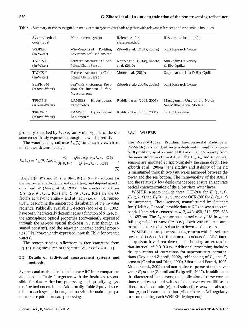
Table 1.Summary of codes assigned to measurement systems/methods together with relevant references and responsible institutes.
System/methodcode (type)
Measurement system References forsystem/method
Responsible institutes(s)
WiSPER(In-Water)
Wire-Stabilized ProfilingEnvironmental Radiometer
Zibordi et al. (2004a, 2009a) Joint Research Centre
TACCS-S(In-Water)
Tethered Attenuation Coef-ficient Chain Sensor
Kratzer et al. (2008), Mooreet al. (2010)
Stockholm University& Bio-Optika
TACCS-P(In-Water)
Tethered Attenuation Coef-ficient Chain Sensor
Moore et al. (2010) Sagremarisco Lda & Bio-Optika
SeaPRISM(Above-Water)
SeaWiFS Photometer Revi-sion for Incident SurfaceMeasurements
Zibordi et al. (2004b, 2009c) Joint Research Centre
TRIOS-B(Above-Water)
RAMSES HyperspectralRadiometers
Ruddick et al. (2005, 2006) Management Unit of the NorthSea Mathematical Models
TRIOS-E(Above-Water)
RAMSES HyperspectralRadiometers
Ruddick et al. (2005, 2006) Tartu Observatory
geometry identified byθ , 1φ, sun zenithθ0, and of the seastate conveniently expressed through the wind speedW .
The water-leaving radianceLw(λ) for a nadir-view direc-tion is then determined by:
Lw(λ) = Lw(θ,1φ,λ)<0
<(θ,W)
Q(θ,1φ,θ0,λ,τa, IOP)
Qn(θ0,λ,τa, IOP),
(5)
where<(θ,W ) and<0 (i.e. <(θ,W ) at θ = 0) account forthe sea surface reflectance and refraction, and depend mainlyon θ and W (Morel et al., 2002). The spectral quantitiesQ(θ,1φ,θ0,λ,τa, IOP) andQn(θ0,λ,τa, IOP) are the Q-factors at viewing angleθ and at nadir (i.e.θ = 0), respec-tively, describing the anisotropic distribution of the in-waterradiance. Publically available Q-factors (Morel et al., 2002)have been theoretically determined as a function ofθ , 1φ, θ0,the atmospheric optical properties (conveniently expressedthrough the aerosol optical thicknessτa, even though as-sumed constant), and the seawater inherent optical proper-ties IOPs (conveniently expressed through Chla for oceanicwaters).
The remote sensing reflectance is then computed fromEq. (3) using measured or theoretical values ofEd(0+,λ).
3.3 Details on individual measurement systems andmethods
Systems and methods included in the ARC inter-comparisonare listed in Table 1 together with the institutes respon-sible for data collection, processing and quantifying sys-tem/method uncertainties. Additionally, Table 2 provides de-tails for each system in conjunction with the main input pa-rameters required for data processing.
3.3.1 WiSPER
The Wire-Stabilized Profiling Environmental Radiometer(WiSPER) is a winched system deployed through a custom-built profiling rig at a speed of 0.1 m s−1 at 7.5 m away fromthe main structure of the AAOT. TheLu, Eu andEd opticalsensors are mounted at approximately the same depth (seeZibordi et al., 2004a). The rigidity and stability of the rigis maintained through two taut wires anchored between thetower and the sea bottom. The immovability of the AAOTand the relatively low deployment speed ensure an accurateoptical characterization of the subsurface water layer.
WiSPER sensors include three OCI-200 forEu(z,λ, t),Ed(z,λ, t) andEd(0+,λ, t), and one OCR-200 forLu(z,λ, t)measurements. These sensors, manufactured by SatlanticInc. (Halifax, Canada), provide data at 6 Hz in seven spectralbands 10 nm wide centered at 412, 443, 490, 510, 555, 665and 683 nm. TheLu sensor has approximately 18◦ in-waterfull-angle field of view (FAFOV). Each WiSPER measure-ment sequence includes data from down- and up-casts.
WiSPER data are processed in agreement with the schemepresented in Sect. 3.1. Radiometric products for ARC inter-comparison have been determined choosing an extrapola-tion interval of 0.3–3.0 m. Additional processing includesthe application of corrections for superstructure perturba-tions (Doyle and Zibordi, 2002), self-shading ofLu andEusensors (Gordon and Ding, 1992; Zibordi and Ferrari, 1995;Mueller et al., 2002), and non-cosine response of the above-waterEd sensor (Zibordi and Bulgarelli, 2007). In addition tothe diameter of the sensors, the application of these correc-tions requires spectral values of the above-water diffuse todirect irradiance ratio (r), and subsurface seawater absorp-tion (a) and beam-attenuation (c) coefficients (all regularlymeasured during each WiSPER deployment).
Ocean Sci., 8, 567–586, 2012 www.ocean-sci.net/8/567/2012/

G. Zibordi et al.: In situ determination of the remote sensing reflectance 571
Table 2. Summary of ARC systems/methods details and of main input quantities required for data processing (symbolsr, a andc indicatethe above-water diffuse to direct irradiance ratio, the seawater absorption and beam attenuation coefficients, respectively).
System/method code Measurement type(radiance)
FAFOV(radiance sensors)
Acquisition frequency andsampling time
Main input quantities
WiSPER In-water manned continu-ous profiles of multispec-tral data in the 400–700 nmspectral region with 10 nmresolution
18◦ (in water) 6 Hz, 160 ms Lu(z,λ, t),Ed(0+,λ, t),a(λ), c(λ), r(λ)
TACCS-S In-water autonomous fixed-depth multispectral data inthe 400–700 nm spectral re-gion with 10 nm resolution
20◦ (in water) 1 Hz, 15 ms(with 1 Hz low-pass filter)
Lu(zi ,λ, t),Ed(zi ,λ, t),Ed(0+,λ, t),a(λ),c(λ)
TACCS-P In-water autonomous fixed-depth hyperspectral data inthe 350–800 nm spectral re-gion with 11 nm resolution
18◦ (in water) 2 Hz, 500 ms(typical forLu(zi ,λ, t))
Lu(zi ,λ, t),Ed(zi ,λ, t),Ed(0+,λ, t),a(λ),c(λ),r(λ)
SeaPRISM Above-water autonomousmultispectral data in the400–1020 nm spectral re-gion with 10 nm resolution
1.2◦ (in air) 1 Hz, 200 ms(spectrally asynchronous)
LT(θ,1φ,λ),Li (θ
′,1φ,λ),Es(θ0,φ0,λ)),W , Chl a, τa(λ)
TRIOS-B Above-water manned hy-perspectral data in the 400–900 nm spectral region with10 nm resolution
7◦ (in air) 0.1 Hz, 250 ms(typical for LT(θ,1φ,λ)during ARC)
LT(θ,1φ,λ),Li (θ
′,1φ, λ),Ed(0+,λ, t),W , Chl a
TRIOS-E Above-water manned hy-perspectral data in the 400–900 nm spectral region with10 nm resolution
7◦ (in air) 0.1 Hz, 250 ms(typical for LT(θ,1φ,λ)during ARC)
LT(θ,1φ,λ),Li (θ
′,1φ, λ),Ed(0+, λ, t),W , Chl a
An analysis of uncertainties of WiSPERRrs(λ) from ARCmeasurements, performed assuming each contribution inde-pendent from the others, indicates values in the range of ap-proximately 4–5 % in the selected spectral region (see Ta-ble 3). The uncertainty sources considered here are (i) un-certainty of the absolute radiance calibration (Hooker et al.,2002b) and immersion factor (Zibordi, 2006) for theLu sen-sor (i.e. 2.7 % and 0.5 %, respectively, composed statisti-cally); (ii) uncertainty of the correction factors applied forremoving self-shading and tower-shading perturbations com-puted as 25 % of the applied corrections; (iii) uncertainty ofthe absolute irradiance calibration of the above-waterEd sen-sor (Hooker et al., 2002b) and uncertainties of the correctionapplied for the non-cosine response of the related irradiancecollectors (Zibordi and Bulgarelli, 2007) (i.e. 2.3 % and 1 %,respectively, composed statistically); (iv) uncertainty in theextrapolation of sub-surface values due to wave perturbationsand changes in illumination and seawater optical propertiesduring profiling cumulatively quantified as the average of thevariation coefficient ofRrs(λ) from replicate measurements.
It is noted that the proposed uncertainty analysis accountsfor fully independent calibrations ofEd andLu sensors (i.e.
Table 3. Uncertainty budget (in percent) forRrs determined fromWiSPER data.
Uncertainty source 443 555 665
Absolute calibration ofLu(z,λ, t) 2.8 2.8 2.8Self- and tower-shading corrections 3.0 1.8 3.2Absolute calibration ofEd(0+,λ, t) 2.5 2.5 2.5Environmental perturbations 0.7 0.7 0.8Quadrature sum 4.9 4.2 5.0
as obtained with different lamps and laboratory set-ups). Theuse of the same calibration lamp and set-up leads to a reduc-tion of approximately 1 % of the quadrature sum of spectraluncertainties for WiSPERRrs(λ).
It is additionally noted that the bottom effects were not in-cluded in the uncertainty analysis being assumed to be negli-gible for the measuring conditions characterizing the ARCinter-comparison. In fact, despite the shallow water depthat the AAOT (i.e. 17 m), an evaluation of bottom perturba-tions based on the scheme proposed by Zibordi et al. (2002a)
www.ocean-sci.net/8/567/2012/ Ocean Sci., 8, 567–586, 2012
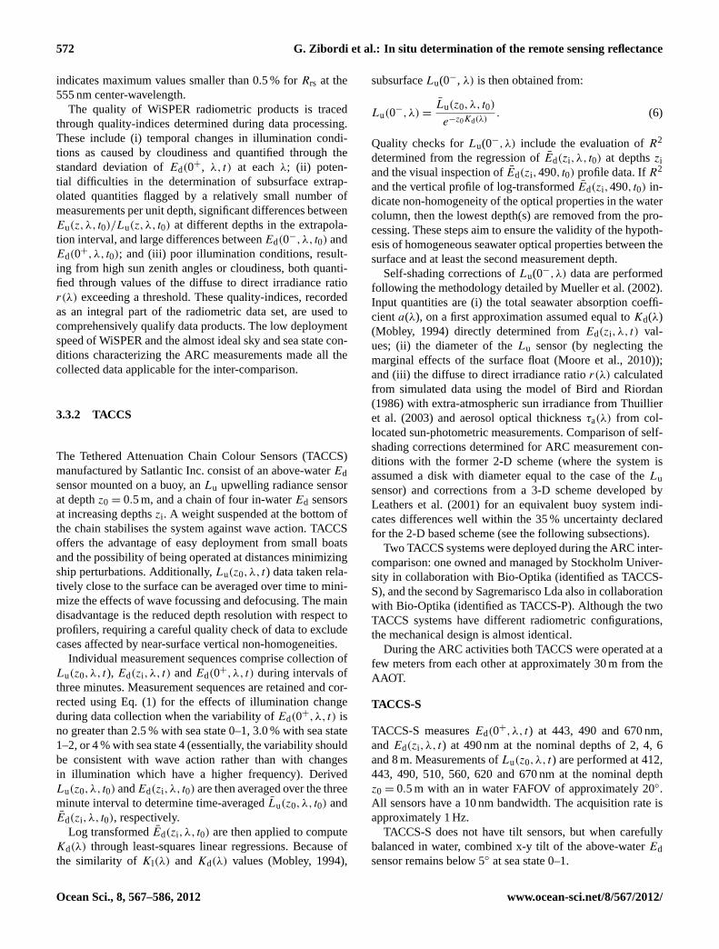
572 G. Zibordi et al.: In situ determination of the remote sensing reflectance
indicates maximum values smaller than 0.5 % forRrs at the555 nm center-wavelength.
The quality of WiSPER radiometric products is tracedthrough quality-indices determined during data processing.These include (i) temporal changes in illumination condi-tions as caused by cloudiness and quantified through thestandard deviation ofEd(0+, λ, t) at eachλ; (ii) poten-tial difficulties in the determination of subsurface extrap-olated quantities flagged by a relatively small number ofmeasurements per unit depth, significant differences betweenEu(z,λ, t0)/Lu(z,λ, t0) at different depths in the extrapola-tion interval, and large differences betweenEd(0−,λ, t0) andEd(0+,λ, t0); and (iii) poor illumination conditions, result-ing from high sun zenith angles or cloudiness, both quanti-fied through values of the diffuse to direct irradiance ratior(λ) exceeding a threshold. These quality-indices, recordedas an integral part of the radiometric data set, are used tocomprehensively qualify data products. The low deploymentspeed of WiSPER and the almost ideal sky and sea state con-ditions characterizing the ARC measurements made all thecollected data applicable for the inter-comparison.
3.3.2 TACCS
The Tethered Attenuation Chain Colour Sensors (TACCS)manufactured by Satlantic Inc. consist of an above-waterEdsensor mounted on a buoy, anLu upwelling radiance sensorat depthz0 = 0.5 m, and a chain of four in-waterEd sensorsat increasing depthszi . A weight suspended at the bottom ofthe chain stabilises the system against wave action. TACCSoffers the advantage of easy deployment from small boatsand the possibility of being operated at distances minimizingship perturbations. Additionally,Lu(z0,λ, t) data taken rela-tively close to the surface can be averaged over time to mini-mize the effects of wave focussing and defocusing. The maindisadvantage is the reduced depth resolution with respect toprofilers, requiring a careful quality check of data to excludecases affected by near-surface vertical non-homogeneities.
Individual measurement sequences comprise collection ofLu(z0,λ, t), Ed(zi,λ, t) andEd(0+,λ, t) during intervals ofthree minutes. Measurement sequences are retained and cor-rected using Eq. (1) for the effects of illumination changeduring data collection when the variability ofEd(0+,λ, t) isno greater than 2.5 % with sea state 0–1, 3.0 % with sea state1–2, or 4 % with sea state 4 (essentially, the variability shouldbe consistent with wave action rather than with changesin illumination which have a higher frequency). DerivedLu(z0,λ, t0) andEd(zi,λ, t0) are then averaged over the threeminute interval to determine time-averagedLu(z0,λ, t0) andEd(zi,λ, t0), respectively.
Log transformedEd(zi,λ, t0) are then applied to computeKd(λ) through least-squares linear regressions. Because ofthe similarity of Kl(λ) and Kd(λ) values (Mobley, 1994),
subsurfaceLu(0−, λ) is then obtained from:
Lu(0−,λ) =
Lu(z0,λ, t0)
e−z0Kd(λ). (6)
Quality checks forLu(0−,λ) include the evaluation ofR2
determined from the regression ofEd(zi,λ, t0) at depthsziand the visual inspection ofEd(zi,490, t0) profile data. IfR2
and the vertical profile of log-transformedEd(zi,490, t0) in-dicate non-homogeneity of the optical properties in the watercolumn, then the lowest depth(s) are removed from the pro-cessing. These steps aim to ensure the validity of the hypoth-esis of homogeneous seawater optical properties between thesurface and at least the second measurement depth.
Self-shading corrections ofLu(0−,λ) data are performedfollowing the methodology detailed by Mueller et al. (2002).Input quantities are (i) the total seawater absorption coeffi-cienta(λ), on a first approximation assumed equal toKd(λ)(Mobley, 1994) directly determined fromEd(zi,λ, t) val-ues; (ii) the diameter of theLu sensor (by neglecting themarginal effects of the surface float (Moore et al., 2010));and (iii) the diffuse to direct irradiance ratior(λ) calculatedfrom simulated data using the model of Bird and Riordan(1986) with extra-atmospheric sun irradiance from Thuillieret al. (2003) and aerosol optical thicknessτa(λ) from col-located sun-photometric measurements. Comparison of self-shading corrections determined for ARC measurement con-ditions with the former 2-D scheme (where the system isassumed a disk with diameter equal to the case of theLusensor) and corrections from a 3-D scheme developed byLeathers et al. (2001) for an equivalent buoy system indi-cates differences well within the 35 % uncertainty declaredfor the 2-D based scheme (see the following subsections).
Two TACCS systems were deployed during the ARC inter-comparison: one owned and managed by Stockholm Univer-sity in collaboration with Bio-Optika (identified as TACCS-S), and the second by Sagremarisco Lda also in collaborationwith Bio-Optika (identified as TACCS-P). Although the twoTACCS systems have different radiometric configurations,the mechanical design is almost identical.
During the ARC activities both TACCS were operated at afew meters from each other at approximately 30 m from theAAOT.
TACCS-S
TACCS-S measuresEd(0+,λ, t) at 443, 490 and 670 nm,andEd(zi,λ, t) at 490 nm at the nominal depths of 2, 4, 6and 8 m. Measurements ofLu(z0,λ, t) are performed at 412,443, 490, 510, 560, 620 and 670 nm at the nominal depthz0 = 0.5 m with an in water FAFOV of approximately 20◦.All sensors have a 10 nm bandwidth. The acquisition rate isapproximately 1 Hz.
TACCS-S does not have tilt sensors, but when carefullybalanced in water, combined x-y tilt of the above-waterEdsensor remains below 5◦ at sea state 0–1.
Ocean Sci., 8, 567–586, 2012 www.ocean-sci.net/8/567/2012/
G. Zibordi et al.: In situ determination of the remote sensing reflectance 573
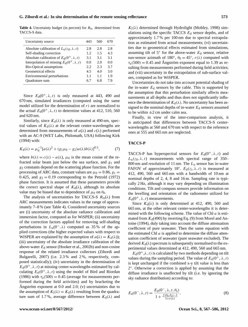
Table 4. Uncertainty budget (in percent) forRrs determined fromTACCS-S data.
Uncertainty source 443 560 670
Absolute calibration ofLu(z0,λ, t) 2.8 2.8 2.8Self-shading correction 1.2 1.5 4.3Absolute calibration ofEd(0+,λ, t) 3.1 3.1 3.1Interpolation of missingEd(0+,λ, t) 0.0 2.0 0.0Bio-Optical assumptions 2.2 2.3 3.7Geometrical effects 4.5 4.0 3.0Environmental perturbations 1.1 1.1 1.9Quadrature sum 6.7 6.8 7.9
Since Ed(0+,λ, t) is only measured at 443, 490 and670 nm, simulated irradiances (computed using the samemodel utilized for the determination ofr) are normalized tothe actualEd(0+,λ, t) to determine values at 412, 510, 560and 620 nm.
Similarly, sinceKd(λ) is only measured at 490 nm, spec-tral values ofKd(λ) at the relevant center-wavelengths aredetermined from measurements ofa(λ) andc(λ) performedwith an AC-9 (WET Labs, Philomath, USA) following Kirk(1994) with:
Kd(λ) = µ−10 [a(λ)2
+ (g1µ0 − g2)a(λ)b(λ)]0.5, (7)
whereb(λ) = c(λ) − a(λ), µ0 is the mean cosine of the re-fracted solar beam just below the sea surface, andg1 andg2 constants depend on the scattering phase function. For theprocessing of ARC data, constant values areµ0 = 0.86,g1 =
0.425, andg2 = 0.19 corresponding to the Petzold (1972)phase function. It is assumed that these parameters providethe correct spectral shape ofKd(λ), although its absolutevalue may be biased due to dependence ofµ0 on θ0.
The analysis of uncertainties for TACCS-SRrs(λ) fromARC measurements indicates values in the range of approx-imately 7–8 % (see Table 4). Considered uncertainty sourcesare (i) uncertainty of the absolute radiance calibration andimmersion factor, computed as for WiSPER; (ii) uncertaintyof the correction factors applied for removing self-shadingperturbations inLu(0−,λ) computed as 35 % of the ap-plied corrections (the higher expected values with respect toWiSPER are explained by the assumption ofa(λ) = Kd(λ));(iii) uncertainty of the absolute irradiance calibration of theabove-waterEd sensor (Hooker et al., 2002b) and non-cosineresponse of the related irradiance collectors (Zibordi andBulgarelli, 2007) (i.e. 2.3 % and 2 %, respectively, com-posed statistically); (iv) uncertainty in the determination ofEd(0+,λ, t) at missing center-wavelengths estimated by cal-culatingEd(0+,λ, t) using the model of Bird and Riordan(1986) withτa(500) = 0.45 (average for measurements per-formed during the field activities) and by bracketing theAngstrom exponent at 0.0 and 2.0; (v) uncertainties due tothe assumption ofKl(λ) = Kd(λ) resulting from the quadra-ture sum of 1.7 %, average difference betweenKd(λ) and
Kl(λ) determined through Hydrolight (Mobley, 1998) sim-ulations using the specific TACCSEd sensor depths, and ofapproximately 1.7 % per 100 nm due to spectral extrapola-tion as estimated from actual measurements; (vi) uncertain-ties due to geometrical effects estimated from simulations,assuming tilt of 5◦ for the above-waterEd sensor, relativesun-sensor azimuth of 180◦, θ0 = 45◦, r(λ) computed withτa(500) = 0.45 andAngstrom exponent equal to 1.39 as re-sulting from measurements performed during field activities;and (vii) uncertainty in the extrapolation of sub-surface val-ues, computed as for WiSPER.
Uncertainties do not take into account potential shading ofthe in-waterEd sensors by the cable. This is supported bythe assumption that this perturbation similarly affects mea-surements at all depths and thus does not significantly influ-ence the determination ofKd(λ). No uncertainty has been as-signed to the nominal depths of in-waterEd sensors assumedto be within±2 cm under calm sea.
Finally, in view of the inter-comparison analysis, itis anticipated that differences between TACCS-S center-wavelengths at 560 and 670 nm with respect to the referenceones at 555 and 665 nm are neglected.
TACCS-P
TACCS-P has hyperspectral sensors forEd(0+,λ, t) andLu(z0,λ, t) measurements with spectral range of 350–800 nm and resolution of 11 nm. TheLu sensor has in-waterFAFOV of approximately 18◦. Ed(zi,λ, t) is measured at412, 490, 560 and 665 nm with a bandwidth of 10 nm atnominal depths of 2, 4, 8 and 16 m. Sampling rate is typi-cally 2 Hz, although it may vary depending on illuminationconditions. Tilt and compass sensors provide information onthe levelling and orientation of the radiometer utilized forEd(0+,λ, t) measurements.
Since Kd(λ) is only determined at 412, 490, 560 and665 nm, at the other relevant center-wavelengths it is deter-mined with the following scheme. The value of Chla is esti-mated fromKd(490) by inverting Eq. (9) from Morel and An-toine (1994), duly taking into account the diffuse attenuationcoefficient of pure seawater. Then the same equation withthe estimated Chla is applied to determine the diffuse atten-uation coefficient of seawater (pure seawater excluded). ThederivedKd(λ) spectrum is subsequently normalised to the ex-perimental values determined at 412, 490, 560 and 665 nm.
Ed(0+,λ, t) is calculated by two methods depending on tiltvalues during the sampling period. The value ofEd(0+, λ, t)
is kept unchanged if the combined x-y tilt value is less than2◦. Otherwise a correction is applied by assuming that thediffuse irradiance is unaffected by tilt (i.e. by ignoring thesky radiance distribution) according to:
Ed(0−,λ, t) =
Ed(0−,λ, t,θs)
1+f (θ0,θs)−1
1+r(λ)
, (8)
www.ocean-sci.net/8/567/2012/ Ocean Sci., 8, 567–586, 2012
574 G. Zibordi et al.: In situ determination of the remote sensing reflectance
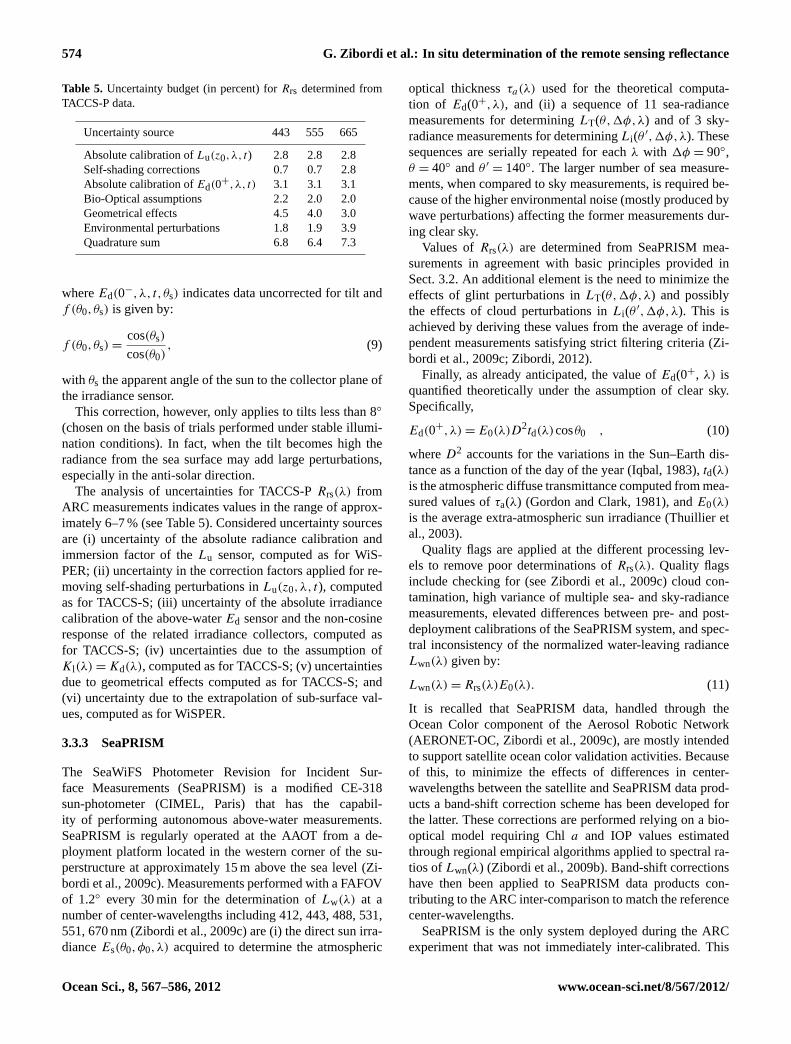
Table 5. Uncertainty budget (in percent) forRrs determined fromTACCS-P data.
Uncertainty source 443 555 665
Absolute calibration ofLu(z0,λ, t) 2.8 2.8 2.8Self-shading corrections 0.7 0.7 2.8Absolute calibration ofEd(0+,λ, t) 3.1 3.1 3.1Bio-Optical assumptions 2.2 2.0 2.0Geometrical effects 4.5 4.0 3.0Environmental perturbations 1.8 1.9 3.9Quadrature sum 6.8 6.4 7.3
whereEd(0−,λ, t,θs) indicates data uncorrected for tilt andf (θ0,θs) is given by:
f (θ0,θs) =cos(θs)
cos(θ0), (9)
with θs the apparent angle of the sun to the collector plane ofthe irradiance sensor.
This correction, however, only applies to tilts less than 8◦
(chosen on the basis of trials performed under stable illumi-nation conditions). In fact, when the tilt becomes high theradiance from the sea surface may add large perturbations,especially in the anti-solar direction.
The analysis of uncertainties for TACCS-PRrs(λ) fromARC measurements indicates values in the range of approx-imately 6–7 % (see Table 5). Considered uncertainty sourcesare (i) uncertainty of the absolute radiance calibration andimmersion factor of theLu sensor, computed as for WiS-PER; (ii) uncertainty in the correction factors applied for re-moving self-shading perturbations inLu(z0,λ, t), computedas for TACCS-S; (iii) uncertainty of the absolute irradiancecalibration of the above-waterEd sensor and the non-cosineresponse of the related irradiance collectors, computed asfor TACCS-S; (iv) uncertainties due to the assumption ofKl(λ) = Kd(λ), computed as for TACCS-S; (v) uncertaintiesdue to geometrical effects computed as for TACCS-S; and(vi) uncertainty due to the extrapolation of sub-surface val-ues, computed as for WiSPER.
3.3.3 SeaPRISM
The SeaWiFS Photometer Revision for Incident Sur-face Measurements (SeaPRISM) is a modified CE-318sun-photometer (CIMEL, Paris) that has the capabil-ity of performing autonomous above-water measurements.SeaPRISM is regularly operated at the AAOT from a de-ployment platform located in the western corner of the su-perstructure at approximately 15 m above the sea level (Zi-bordi et al., 2009c). Measurements performed with a FAFOVof 1.2◦ every 30 min for the determination ofLw(λ) at anumber of center-wavelengths including 412, 443, 488, 531,551, 670 nm (Zibordi et al., 2009c) are (i) the direct sun irra-dianceEs(θ0,φ0,λ) acquired to determine the atmospheric
optical thicknessτa(λ) used for the theoretical computa-tion of Ed(0+,λ), and (ii) a sequence of 11 sea-radiancemeasurements for determiningLT(θ,1φ,λ) and of 3 sky-radiance measurements for determiningLi(θ ′,1φ,λ). Thesesequences are serially repeated for eachλ with 1φ = 90◦,θ = 40◦ andθ ′
= 140◦. The larger number of sea measure-ments, when compared to sky measurements, is required be-cause of the higher environmental noise (mostly produced bywave perturbations) affecting the former measurements dur-ing clear sky.
Values ofRrs(λ) are determined from SeaPRISM mea-surements in agreement with basic principles provided inSect. 3.2. An additional element is the need to minimize theeffects of glint perturbations inLT(θ,1φ,λ) and possiblythe effects of cloud perturbations inLi(θ ′,1φ,λ). This isachieved by deriving these values from the average of inde-pendent measurements satisfying strict filtering criteria (Zi-bordi et al., 2009c; Zibordi, 2012).
Finally, as already anticipated, the value ofEd(0+, λ) isquantified theoretically under the assumption of clear sky.Specifically,
Ed(0+,λ) = E0(λ)D2td(λ)cosθ0 , (10)
whereD2 accounts for the variations in the Sun–Earth dis-tance as a function of the day of the year (Iqbal, 1983),td(λ)
is the atmospheric diffuse transmittance computed from mea-sured values ofτa(λ) (Gordon and Clark, 1981), andE0(λ)
is the average extra-atmospheric sun irradiance (Thuillier etal., 2003).
Quality flags are applied at the different processing lev-els to remove poor determinations ofRrs(λ). Quality flagsinclude checking for (see Zibordi et al., 2009c) cloud con-tamination, high variance of multiple sea- and sky-radiancemeasurements, elevated differences between pre- and post-deployment calibrations of the SeaPRISM system, and spec-tral inconsistency of the normalized water-leaving radianceLwn(λ) given by:
Lwn(λ) = Rrs(λ)E0(λ). (11)
It is recalled that SeaPRISM data, handled through theOcean Color component of the Aerosol Robotic Network(AERONET-OC, Zibordi et al., 2009c), are mostly intendedto support satellite ocean color validation activities. Becauseof this, to minimize the effects of differences in center-wavelengths between the satellite and SeaPRISM data prod-ucts a band-shift correction scheme has been developed forthe latter. These corrections are performed relying on a bio-optical model requiring Chla and IOP values estimatedthrough regional empirical algorithms applied to spectral ra-tios ofLwn(λ) (Zibordi et al., 2009b). Band-shift correctionshave then been applied to SeaPRISM data products con-tributing to the ARC inter-comparison to match the referencecenter-wavelengths.
SeaPRISM is the only system deployed during the ARCexperiment that was not immediately inter-calibrated. This
Ocean Sci., 8, 567–586, 2012 www.ocean-sci.net/8/567/2012/
G. Zibordi et al.: In situ determination of the remote sensing reflectance 575
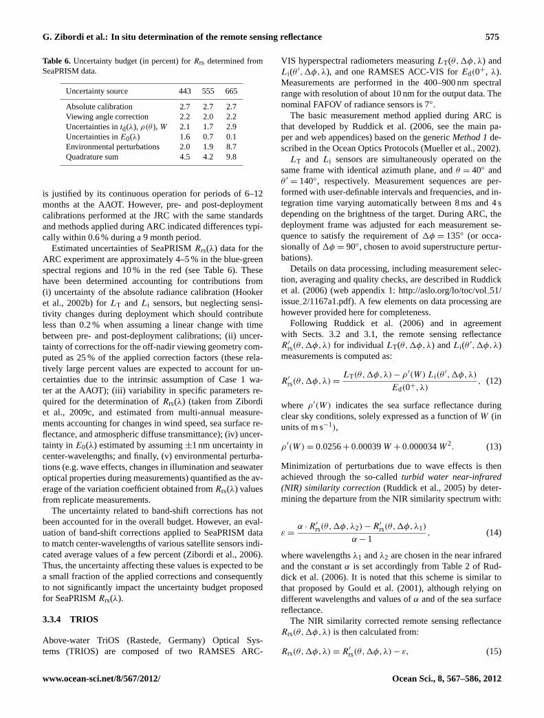
Table 6. Uncertainty budget (in percent) forRrs determined fromSeaPRISM data.
Uncertainty source 443 555 665
Absolute calibration 2.7 2.7 2.7Viewing angle correction 2.2 2.0 2.2Uncertainties intd(λ), ρ(θ ), W 2.1 1.7 2.9Uncertainties inE0(λ) 1.6 0.7 0.1Environmental perturbations 2.0 1.9 8.7Quadrature sum 4.5 4.2 9.8
is justified by its continuous operation for periods of 6–12months at the AAOT. However, pre- and post-deploymentcalibrations performed at the JRC with the same standardsand methods applied during ARC indicated differences typi-cally within 0.6 % during a 9 month period.
Estimated uncertainties of SeaPRISMRrs(λ) data for theARC experiment are approximately 4–5 % in the blue-greenspectral regions and 10 % in the red (see Table 6). Thesehave been determined accounting for contributions from(i) uncertainty of the absolute radiance calibration (Hookeret al., 2002b) forLT andLi sensors, but neglecting sensi-tivity changes during deployment which should contributeless than 0.2 % when assuming a linear change with timebetween pre- and post-deployment calibrations; (ii) uncer-tainty of corrections for the off-nadir viewing geometry com-puted as 25 % of the applied correction factors (these rela-tively large percent values are expected to account for un-certainties due to the intrinsic assumption of Case 1 wa-ter at the AAOT); (iii) variability in specific parameters re-quired for the determination ofRrs(λ) (taken from Zibordiet al., 2009c, and estimated from multi-annual measure-ments accounting for changes in wind speed, sea surface re-flectance, and atmospheric diffuse transmittance); (iv) uncer-tainty in E0(λ) estimated by assuming±1 nm uncertainty incenter-wavelengths; and finally, (v) environmental perturba-tions (e.g. wave effects, changes in illumination and seawateroptical properties during measurements) quantified as the av-erage of the variation coefficient obtained fromRrs(λ) valuesfrom replicate measurements.
The uncertainty related to band-shift corrections has notbeen accounted for in the overall budget. However, an eval-uation of band-shift corrections applied to SeaPRISM datato match center-wavelengths of various satellite sensors indi-cated average values of a few percent (Zibordi et al., 2006).Thus, the uncertainty affecting these values is expected to bea small fraction of the applied corrections and consequentlyto not significantly impact the uncertainty budget proposedfor SeaPRISMRrs(λ).
3.3.4 TRIOS
Above-water TriOS (Rastede, Germany) Optical Sys-tems (TRIOS) are composed of two RAMSES ARC-
VIS hyperspectral radiometers measuringLT(θ,1φ,λ) andLi(θ ′,1φ,λ), and one RAMSES ACC-VIS forEd(0+, λ).Measurements are performed in the 400–900 nm spectralrange with resolution of about 10 nm for the output data. Thenominal FAFOV of radiance sensors is 7◦.
The basic measurement method applied during ARC isthat developed by Ruddick et al. (2006, see the main pa-per and web appendices) based on the genericMethod 1de-scribed in the Ocean Optics Protocols (Mueller et al., 2002).
LT and Li sensors are simultaneously operated on thesame frame with identical azimuth plane, andθ = 40◦ andθ ′
= 140◦, respectively. Measurement sequences are per-formed with user-definable intervals and frequencies, and in-tegration time varying automatically between 8 ms and 4 sdepending on the brightness of the target. During ARC, thedeployment frame was adjusted for each measurement se-quence to satisfy the requirement of1φ = 135◦ (or occa-sionally of1φ = 90◦, chosen to avoid superstructure pertur-bations).
Details on data processing, including measurement selec-tion, averaging and quality checks, are described in Ruddicket al. (2006) (web appendix 1:http://aslo.org/lo/toc/vol51/issue2/1167a1.pdf). A few elements on data processing arehowever provided here for completeness.
Following Ruddick et al. (2006) and in agreementwith Sects. 3.2 and 3.1, the remote sensing reflectanceR′
rs(θ,1φ,λ) for individual LT(θ,1φ,λ) andLi(θ ′,1φ,λ)measurements is computed as:
R′rs(θ,1φ,λ) =
LT(θ,1φ,λ) − ρ′(W) Li(θ′,1φ,λ)
Ed(0+,λ), (12)
where ρ′(W) indicates the sea surface reflectance duringclear sky conditions, solely expressed as a function ofW (inunits of m s−1),
ρ′(W) = 0.0256+ 0.00039W + 0.000034W2. (13)
Minimization of perturbations due to wave effects is thenachieved through the so-calledturbid water near-infrared(NIR) similarity correction(Ruddick et al., 2005) by deter-mining the departure from the NIR similarity spectrum with:
ε =α · R′
rs(θ,1φ,λ2) − R′rs(θ,1φ,λ1)
α − 1, (14)
where wavelengthsλ1 andλ2 are chosen in the near infraredand the constantα is set accordingly from Table 2 of Rud-dick et al. (2006). It is noted that this scheme is similar tothat proposed by Gould et al. (2001), although relying ondifferent wavelengths and values ofα and of the sea surfacereflectance.
The NIR similarity corrected remote sensing reflectanceRrs(θ,1φ,λ) is then calculated from:
Rrs(θ,1φ,λ) = R′rs(θ,1φ,λ) − ε, (15)
www.ocean-sci.net/8/567/2012/ Ocean Sci., 8, 567–586, 2012
576 G. Zibordi et al.: In situ determination of the remote sensing reflectance
Table 7. Uncertainty budget (in percent) forRrs determined fromTRIOS-B data.
Uncertainty source 443 555 665
System calibration 2.0 2.0 2.0Straylight effects 5.0 0.5 1.0Polarization effects 1.0 1.0 1.0Non-cosine response ofEd 2.0 2.0 2.0Sky-light correction 2.0 1.0 2.9Viewing angle correction 1.5 1.5 1.5Quadrature sum 6.3 3.5 4.5
where the correction is assumed spectrally invariant. The cor-responding NIR similarity corrected water-leaving radianceis calculated as:
Lw(θ,1φ,λ) = Ed(0+,λ)Rrs(θ,1φ,λ). (16)
A number of data products (i.e. 5) are then averaged to obtainthe NIR similarity correctedLw(θ,1φ,λ).
For ARC measurements a viewing angle correction is alsoapplied toLw(θ,1φ,λ) in agreement with Eq. (5) to deter-mine Lw(λ). The values of Chla required for such a cor-rection were estimated using a regional band-ratio algorithm(Berthon and Zibordi, 2004).
Two TRIOS systems were deployed at the AAOT adjacentto the SeaPRISM during the ARC experiment: one ownedand handled by the Management Unit of the North Sea Math-ematical Models (identified as TRIOS-B) and the other byTartu Observatory (identified as TRIOS-E). The two sys-tems are equivalent, but measurements have been performedindependently and reduced by applying slightly differentschemes, corresponding to the standard practices of the twoinstitutions and with some differences in the approach for un-certainty estimate. These elements are separately presentedin the following subsections.
Data for inter-comparisons have been constructed by lin-early interpolating quality checked products at the referencecenter-wavelengths.
TRIOS-B
Ed(0+,λ), LT(θ,1φ,λ) and Li(θ ′,1φ,λ) are simultane-ously acquired for 10 min taking measurements every 10 s.Calibrated data are quality checked for incomplete and for in-dividual measurements differing by more than 25 % from theneighbouring ones. In the case of ARC data, quality check-ing led to the rejection of 1 % of measurements. The NIRsimilarity correction is then performed usingλ1 = 780 nm,λ2 = 870 nm, andα = 1.91 (Ruddick et al., 2006).
Estimated uncertainties ofRrs(λ) for TRIOS-B approxi-mately vary between 4 and 6 % in the spectral range of in-terest (see Table 7). The considered uncertainty sources are(i) uncertainty of system calibration determined assumingthe same irradiance standard is utilized for the absolute cal-
Table 8. Uncertainty budget (in percent) forRrs determined fromTRIOS-E data.
Uncertainty source 443 555 665
System calibration 2.0 2.0 2.0Straylight effects 5.0 0.5 1.0Polarization effects 1.0 1.0 1.0NIR similarity correction 0.5 0.4 2.2Viewing angle correction 1.5 1.7 1.3Non-cosine response ofEd 2.0 2.0 2.0Environmental perturbations 1.8 1.0 2.0Quadrature sum 6.3 3.6 4.5
ibration of theEd, LT, and Li sensors, and thus only ac-counting for effects of mechanical setup, inadequate baf-fling and reference plaque uncertainties (see Hooker et al.,2002b); (ii) uncertainty due to straylight effects quantifiedthrough the application of laboratory characterizations per-formed for RAMSESEd, LT and Li sensors (Ansko, un-published); (iii) polarization effects quantified as the max-imum sensitivity to polarization determined through labo-ratory characterizations for RAMSESLT and Li sensors(Ruddick, unpublished); (iv) effects of non-cosine responseof the above-waterEd collector determined from labora-tory measurements (Ruddick, unpublished); (v) uncertaintyin sky-light correction quantified in agreement with Ruddicket al. (2006) as a function of the uncertainty inρ′(W); and(vi) uncertainty in the correction for off-nadir viewing anglequantified as 25 % of the applied corrections, and exhibit-ing different values than those proposed for SeaPRISM be-cause of the diverse viewing geometry generally relying on1φ = 135◦ instead of1φ = 90◦.
It is noted that the uncertainty for the sky glint correction ishighly dependent on sea state, and the relative percent valueof this uncertainty is inversely proportional toRrs(θ,1φ,λ)
(see web appendix 2 of Ruddick et al., 2006). The valuesgiven here have, therefore, been calculated very specificallyaccounting for the sea state recorded during the ARC activ-ities and the observed water-leaving radiances (see Sect. 4).Measurements performed in different waters or sea state con-ditions may lead to different uncertainties.
TRIOS-E
The LT(θ,1φ,λ), Li(θ ′,1φ,λ), and Ed(0+,λ) measure-ment sequences are simultaneously recorded every 10 sec-onds for approximately 6 min, commonly using1φ = 135◦.The NIR similarity correction is performed withλ1 =
720 nm,λ2 = 780 nm andα = 2.35 (Ruddick et al., 2006).The rationale for choosing this wavelength pair, differentfrom that applied for TRIOS-B, is the higher signal tonoise ratio characterizing measurements at the shorter wave-lengths.
Ocean Sci., 8, 567–586, 2012 www.ocean-sci.net/8/567/2012/
G. Zibordi et al.: In situ determination of the remote sensing reflectance 577
0.00
0.25
0.50
0.75
1.00
400 500 600 700
L w [m
W cm
-2
m-1
sr-1
]
Wavelength [nm]
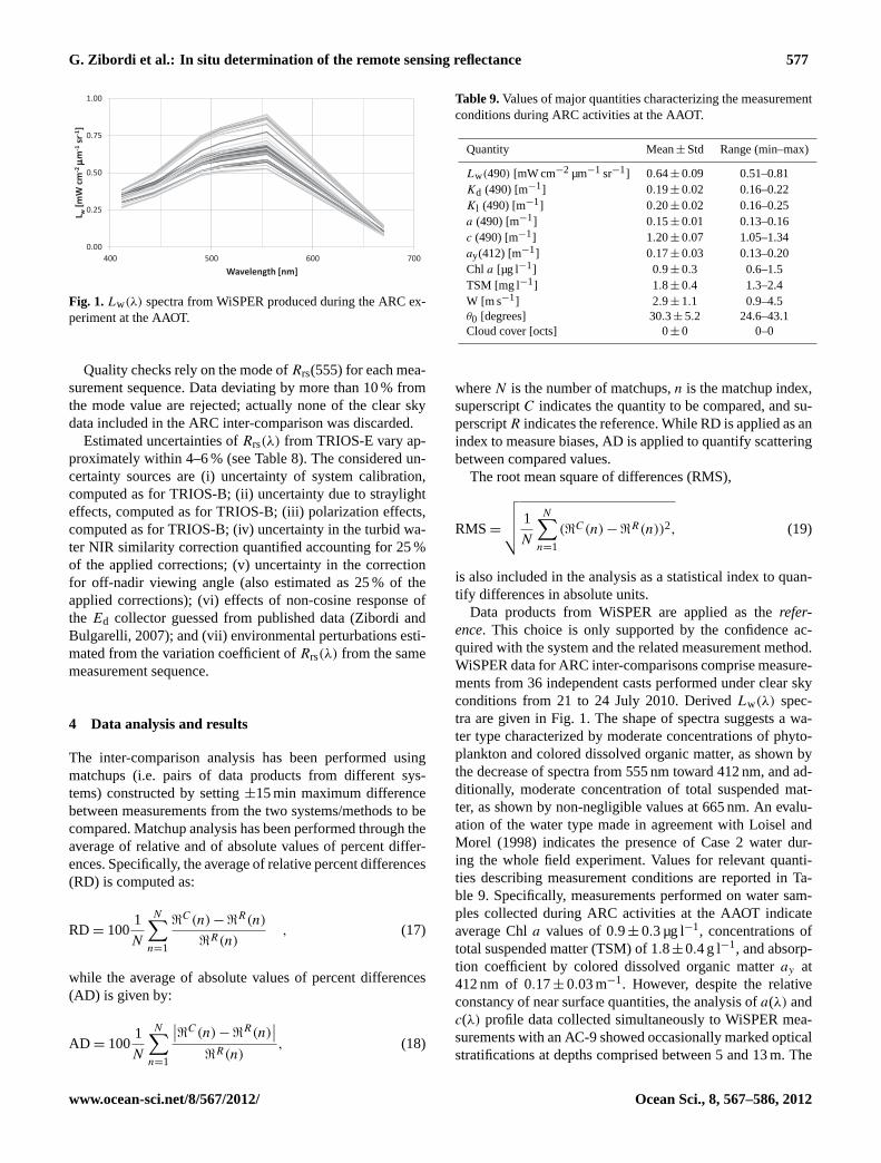
Fig. 1.Lw(λ) spectra from WiSPER produced during the ARC ex-periment at the AAOT.
Quality checks rely on the mode ofRrs(555) for each mea-surement sequence. Data deviating by more than 10 % fromthe mode value are rejected; actually none of the clear skydata included in the ARC inter-comparison was discarded.
Estimated uncertainties ofRrs(λ) from TRIOS-E vary ap-proximately within 4–6 % (see Table 8). The considered un-certainty sources are (i) uncertainty of system calibration,computed as for TRIOS-B; (ii) uncertainty due to straylighteffects, computed as for TRIOS-B; (iii) polarization effects,computed as for TRIOS-B; (iv) uncertainty in the turbid wa-ter NIR similarity correction quantified accounting for 25 %of the applied corrections; (v) uncertainty in the correctionfor off-nadir viewing angle (also estimated as 25 % of theapplied corrections); (vi) effects of non-cosine response ofthe Ed collector guessed from published data (Zibordi andBulgarelli, 2007); and (vii) environmental perturbations esti-mated from the variation coefficient ofRrs(λ) from the samemeasurement sequence.
4 Data analysis and results
The inter-comparison analysis has been performed usingmatchups (i.e. pairs of data products from different sys-tems) constructed by setting±15 min maximum differencebetween measurements from the two systems/methods to becompared. Matchup analysis has been performed through theaverage of relative and of absolute values of percent differ-ences. Specifically, the average of relative percent differences(RD) is computed as:
RD = 1001
N
N∑n=1
<C(n) − <
R(n)
<R(n), (17)
while the average of absolute values of percent differences(AD) is given by:
AD = 1001
N
N∑n=1
∣∣<C(n) − <R(n)
∣∣<R(n)
, (18)
Table 9.Values of major quantities characterizing the measurementconditions during ARC activities at the AAOT.
Quantity Mean± Std Range (min–max)
Lw(490) [mW cm−2 µm−1 sr−1] 0.64± 0.09 0.51–0.81Kd (490) [m−1] 0.19± 0.02 0.16–0.22Kl (490) [m−1] 0.20± 0.02 0.16–0.25a (490) [m−1] 0.15± 0.01 0.13–0.16c (490) [m−1] 1.20± 0.07 1.05–1.34ay(412) [m−1] 0.17± 0.03 0.13–0.20Chl a [µg l−1] 0.9± 0.3 0.6–1.5TSM [mg l−1] 1.8± 0.4 1.3–2.4W [m s−1] 2.9± 1.1 0.9–4.5θ0 [degrees] 30.3± 5.2 24.6–43.1Cloud cover [octs] 0± 0 0–0
whereN is the number of matchups,n is the matchup index,superscriptC indicates the quantity to be compared, and su-perscriptR indicates the reference. While RD is applied as anindex to measure biases, AD is applied to quantify scatteringbetween compared values.
The root mean square of differences (RMS),
RMS=
√√√√ 1
N
N∑n=1
(<C(n) − <R(n))2, (19)
is also included in the analysis as a statistical index to quan-tify differences in absolute units.
Data products from WiSPER are applied as therefer-ence. This choice is only supported by the confidence ac-quired with the system and the related measurement method.WiSPER data for ARC inter-comparisons comprise measure-ments from 36 independent casts performed under clear skyconditions from 21 to 24 July 2010. DerivedLw(λ) spec-tra are given in Fig. 1. The shape of spectra suggests a wa-ter type characterized by moderate concentrations of phyto-plankton and colored dissolved organic matter, as shown bythe decrease of spectra from 555 nm toward 412 nm, and ad-ditionally, moderate concentration of total suspended mat-ter, as shown by non-negligible values at 665 nm. An evalu-ation of the water type made in agreement with Loisel andMorel (1998) indicates the presence of Case 2 water dur-ing the whole field experiment. Values for relevant quanti-ties describing measurement conditions are reported in Ta-ble 9. Specifically, measurements performed on water sam-ples collected during ARC activities at the AAOT indicateaverage Chla values of 0.9± 0.3 µg l−1, concentrations oftotal suspended matter (TSM) of 1.8±0.4 g l−1, and absorp-tion coefficient by colored dissolved organic matteray at412 nm of 0.17± 0.03 m−1. However, despite the relativeconstancy of near surface quantities, the analysis ofa(λ) andc(λ) profile data collected simultaneously to WiSPER mea-surements with an AC-9 showed occasionally marked opticalstratifications at depths comprised between 5 and 13 m. The
www.ocean-sci.net/8/567/2012/ Ocean Sci., 8, 567–586, 2012
578 G. Zibordi et al.: In situ determination of the remote sensing reflectance
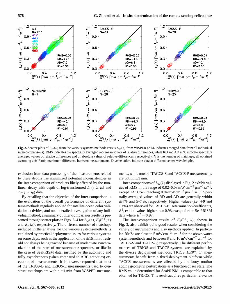
Fig. 2.Scatter plots ofLw(λ) from the various systems/methods versusLw(λ) from WiSPER (ALL indicates merged data from all individualinter-comparisons). RMS indicates the spectrally averaged root mean square of relative differences, while RD and AD in % indicate spectrallyaveraged values of relative differences and of absolute values of relative differences, respectively.N is the number of matchups, all obtainedassuming a±15 min maximum difference between measurements. Diverse colors indicate data at different center-wavelengths.
exclusion from data processing of the measurements relatedto these depths has minimized potential inconsistencies inthe inter-comparison of products likely affected by the non-linear decay with depth of log-transformedLu(z,λ, t0) andEd(z,λ, t0) data.
By recalling that the objective of the inter-comparison isthe evaluation of the overall performance of different sys-tems/methods regularly applied for satellite ocean color vali-dation activities, and not a detailed investigation of any indi-vidual method, a summary of inter-comparison results is pre-sented through scatter plots in Figs. 2–4 forLw(λ), Ed(0+,λ)
andRrs(λ), respectively. The different number of matchupsincluded in the analysis for the various systems/methods isexplained by practical deployment issues for various systemson some days, such as the application of the±15 min thresh-old not always being reached because of inadequate synchro-nization of the start of measurement sequences, or like inthe case of SeaPRISM data, justified by the automatic andfully asynchronous (when compared to ARC activities) ex-ecution of measurements. It is however reported that mostof the TRIOS-B and TRIOS-E measurements used to con-struct matchups are within±1 min from WiSPER measure-
ments, while most of TACCS-S and TACCS-P measurementsare within±3 min.
Inter-comparisons ofLw(λ) displayed in Fig. 2 exhibit val-ues of RMS in the range of 0.02–0.03 mW cm−2 µm−1 sr−1,except TACCS-P reaching 0.04 mW cm−2 µm−1 sr−1. Spec-trally averaged values of RD and AD are generally within±4 % and 5–7 %, respectively. Higher values (i.e.+9 and10 %) are observed for TACCS-P. Determination coefficients,R2, exhibit values higher than 0.98, except for the SeaPRISMdata whereR2
= 0.97.The inter-comparison results ofEd(0+, λ), shown in
Fig. 3, also exhibit quite good results when considering thevariety of instruments and also methods applied. In particu-lar, RMSs are close to 5 mW cm−2 µm−1 for the above-watersystems/methods and between 8 and 10 mW cm−2 µm−1 forTACCS-S and TACCS-P, respectively. The different perfor-mances of TRIOS and TACCS systems are explained bythe diverse deployment methods; TRIOSEd(0+, λ) mea-surements benefit from a fixed deployment platform whileTACCS measurements are affected by the buoy motionadding geometric perturbations as a function of sea state. TheRMS value determined for SeaPRISM is comparable to thatobtained for TRIOS. This result acquires particular relevance
Ocean Sci., 8, 567–586, 2012 www.ocean-sci.net/8/567/2012/
G. Zibordi et al.: In situ determination of the remote sensing reflectance 579
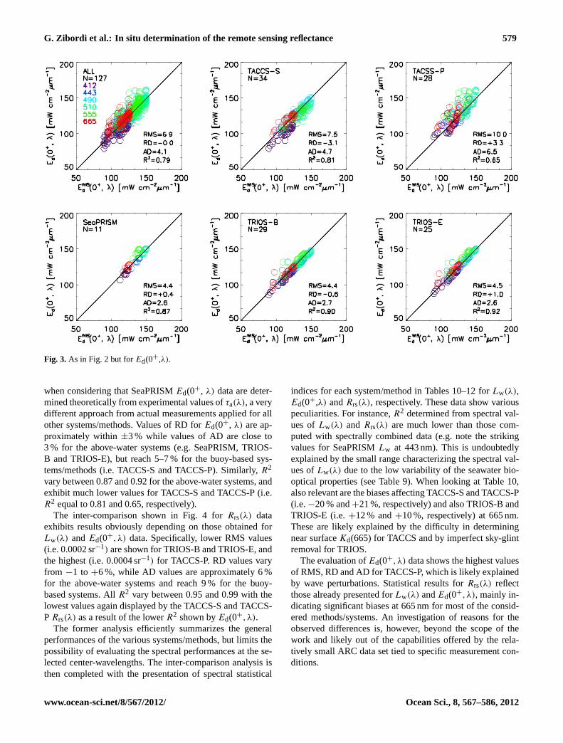
Fig. 3.As in Fig. 2 but forEd(0+,λ).
when considering that SeaPRISMEd(0+, λ) data are deter-mined theoretically from experimental values ofτa(λ), a verydifferent approach from actual measurements applied for allother systems/methods. Values of RD forEd(0+, λ) are ap-proximately within±3 % while values of AD are close to3 % for the above-water systems (e.g. SeaPRISM, TRIOS-B and TRIOS-E), but reach 5–7 % for the buoy-based sys-tems/methods (i.e. TACCS-S and TACCS-P). Similarly,R2
vary between 0.87 and 0.92 for the above-water systems, andexhibit much lower values for TACCS-S and TACCS-P (i.e.R2 equal to 0.81 and 0.65, respectively).
The inter-comparison shown in Fig. 4 forRrs(λ) dataexhibits results obviously depending on those obtained forLw(λ) andEd(0+,λ) data. Specifically, lower RMS values(i.e. 0.0002 sr−1) are shown for TRIOS-B and TRIOS-E, andthe highest (i.e. 0.0004 sr−1) for TACCS-P. RD values varyfrom −1 to +6 %, while AD values are approximately 6 %for the above-water systems and reach 9 % for the buoy-based systems. AllR2 vary between 0.95 and 0.99 with thelowest values again displayed by the TACCS-S and TACCS-PRrs(λ) as a result of the lowerR2 shown byEd(0+,λ).
The former analysis efficiently summarizes the generalperformances of the various systems/methods, but limits thepossibility of evaluating the spectral performances at the se-lected center-wavelengths. The inter-comparison analysis isthen completed with the presentation of spectral statistical
indices for each system/method in Tables 10–12 forLw(λ),Ed(0+,λ) andRrs(λ), respectively. These data show variouspeculiarities. For instance,R2 determined from spectral val-ues ofLw(λ) and Rrs(λ) are much lower than those com-puted with spectrally combined data (e.g. note the strikingvalues for SeaPRISMLw at 443 nm). This is undoubtedlyexplained by the small range characterizing the spectral val-ues ofLw(λ) due to the low variability of the seawater bio-optical properties (see Table 9). When looking at Table 10,also relevant are the biases affecting TACCS-S and TACCS-P(i.e.−20 % and+21 %, respectively) and also TRIOS-B andTRIOS-E (i.e.+12 % and+10 %, respectively) at 665 nm.These are likely explained by the difficulty in determiningnear surfaceKd(665) for TACCS and by imperfect sky-glintremoval for TRIOS.
The evaluation ofEd(0+,λ) data shows the highest valuesof RMS, RD and AD for TACCS-P, which is likely explainedby wave perturbations. Statistical results forRrs(λ) reflectthose already presented forLw(λ) andEd(0+,λ), mainly in-dicating significant biases at 665 nm for most of the consid-ered methods/systems. An investigation of reasons for theobserved differences is, however, beyond the scope of thework and likely out of the capabilities offered by the rela-tively small ARC data set tied to specific measurement con-ditions.
www.ocean-sci.net/8/567/2012/ Ocean Sci., 8, 567–586, 2012

580 G. Zibordi et al.: In situ determination of the remote sensing reflectance
Fig. 4.As in Fig. 2 but forRrs(λ).
4.1 Discussion
Results for the ARC inter-comparison illustrate the bestthat can be achieved with the considered systems/methodsunder almost ideal measurement circumstances driven byfavourable deployment capabilities as offered by the stabilityof the AAOT platform (i.e. makingEd(0+, λ) measurementsunaffected by tilt, when performed from the main superstruc-ture), almost ideal environmental conditions characterizedby relatively low sun zenith angles, clear sky and moder-ately low sea state, and finally inter-calibration of measure-ment systems. By solely considering this latter element, itis recalled that the inter-calibration removes potential biasesin derived radiometric products generated by out-of-date orinaccurate calibrations. The comparison of absolute coeffi-cients obtained at the JRC during the inter-calibration withthose previously applied for the various systems includedin ARC has shown minimum differences of 1–2 % but alsovalues exceeding 4 % for individual radiometers. These sec-ond relatively high differences, if not removed, would signifi-cantly degrade the inter-comparison for one of the consideredsystems/methods.
Processing of data from in-water systems/methods re-quires values ofa(λ) and c(λ). Differently, processing ofdata from above-water systems/methods requires valuesW
and Chla. The impact of uncertainties of these input quanti-
ties is accounted for in theRrs(λ) uncertainty budget for eachsystem/method. It is however of interest to evaluate the im-pact of important quantities such as Chla utilized to correctfor the off-nadir viewing geometry ofLw(θ,1φ,λ). In thepresent exercise Chla was determined for all systems usinga regional algorithm (see Berthon and Zibordi, 2004) appliedto Rrs(λ) ratios. The average and the standard deviation ofvalues computed for ARC measurements are 1.9±0.2 µg l−1.The corresponding values for actual concentrations deter-mined from water samples through High Performance LiquidChromatography (HPLC) are 0.9± 0.3 µg l−1. The analysisof TRIOS-B data indicates that the different Chla estimatesgive viewing angle corrections differing by less than 1 % for1φ = 135◦ and varying between 1 and 4 % for1φ = 90◦.However, the overall effect onRrs(λ) inter-comparisons iswell within the assumed uncertainties. In fact, when usingmeasured Chla instead of the computed values, TRIOS-E, TRIOS-B and SeaPRISM results indicate an increase of0.5 %, 0.9 % and 1.2 %, respectively, for the spectrally av-eraged RD, and no significant change for the other statisticalquantities. Differences among spectrally averaged RD for thevarious systems/methods are explained by the different mea-surement sequences included in the inter-comparison com-prising diverse viewing geometries.
In order to evaluate the consistency of the overall inter-comparison results illustrated in Sect. 4, Table 13 displays
Ocean Sci., 8, 567–586, 2012 www.ocean-sci.net/8/567/2012/
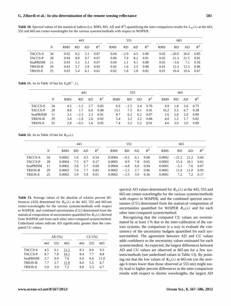
G. Zibordi et al.: In situ determination of the remote sensing reflectance 581
Table 10.Spectral values of the statistical indices (i.e. RMS, RD, AD andR2) quantifying the inter-comparison results forLw(λ) at the 443,555 and 665 nm center-wavelengths for the various systems/methods with respect to WiSPER.
443 555 665
N RMS RD AD R2 RMS RD AD R2 RMS RD AD R2
TACCS-S 34 0.02 0.2 3.1 0.87 0.04−2.9 4.5 0.90 0.02 −20.0 20.0 0.85TACCS-P 28 0.04 8.8 9.7 0.67 0.06 7.9 8.2 0.91 0.02 21.3 21.5 0.81SeaPRISM 11 0.03 1.5 5.1 0.07 0.04 1.1 4.1 0.88 0.01−3.6 7.1 0.56TRIOS-B 29 0.03 5.7 5.9 0.92 0.02 1.6 2.5 0.98 0.01 12.3 12.3 0.96TRIOS-E 25 0.03 5.4 6.1 0.61 0.02 1.8 2.8 0.82 0.01 10.4 10.4 0.67
Table 11.As in Table 10 but forEd(0+,λ).
443 555 665
N RMS RD AD R2 RMS RD AD R2 RMS RD AD R2
TACCS-S 34 4.5 −1.2 2.7 0.85 6.0 −2.5 3.4 0.76 4.9 1.8 3.6 0.75TACCS-P 28 8.8 1.7 6.0 0.48 13.1 7.5 8.1 0.41 10.2 5.5 6.7 0.38SeaPRISM 11 3.5 −2.3 2.3 0.91 8.7 6.2 6.2 0.87 2.6 2.0 2.0 0.89TRIOS-B 29 3.8 −1.8 2.6 0.92 5.4 3.2 3.2 0.86 4.0 1.2 1.7 0.82TRIOS-E 25 2.8 −0.5 1.6 0.95 7.4 5.2 5.2 0.91 4.6 3.0 3.0 0.89
Table 12.As in Table 10 but forRrs(λ).
443 555 665
N RMS RD AD R2 RMS RD AD R2 RMS RD AD R2
TACCS-S 34 0.0002 1.6 4.5 0.54 0.0004−0.2 6.1 0.68 0.0002 −21.2 21.2 0.66TACCS-P 28 0.0004 7.5 8.7 0.17 0.0005 0.9 7.8 0.65 0.0002 15.4 16.1 0.61SeaPRISM 11 0.0002 3.8 5.7 0.68 0.0004−4.8 6.0 0.94 0.0001 −5.5 7.6 0.67TRIOS-B 29 0.0003 7.6 7.7 0.83 0.0002−1.5 2.7 0.96 0.0001 11.0 11.0 0.95TRIOS-E 25 0.0002 5.9 5.9 0.01 0.0002−3.3 3.9 0.36 0.0001 7.2 7.2 0.17
Table 13. Average values of the absolute of relative percent dif-ferences (AD) determined forRrs(λ) at the 443, 555 and 665 nmcenter-wavelengths for the various systems/methods with respectto WiSPER, and combined uncertainties (CU) determined from thestatistical composition of uncertainties quantified forRrs(λ) derivedfrom WiSPER and from each other inter-compared system/method.Underlined values indicate AD significantly greater than the com-puted CU values.
AD [%] CU [%]
443 555 665 443 555 665
TACCS-S 4.5 6.1 21.2 8.3 8.0 9.3TACCS-P 8.7 7.8 16.1 8.4 7.7 8.8SeaPRISM 5.7 6.0 7.6 6.9 6.0 11.0TRIOS-B 7.7 2.7 11.0 8.0 5.5 6.7TRIOS-E 5.9 3.9 7.2 8.0 5.5 6.7
spectral AD values determined forRrs(λ) at the 443, 555 and665 nm center-wavelengths for the various systems/methodswith respect to WiSPER, and the combined spectral uncer-tainties (CU) determined from the statistical composition ofuncertainties quantified for WiSPERRrs(λ) and for eachother inter-compared system/method.
Recognizing that the computed CU values are overesti-mated by at least 1 % due to the inter-calibration of the var-ious systems, the comparison is a way to evaluate the con-sistency of the uncertainty budgets quantified for each sys-tem/method. The agreement between AD and CU valuesadds confidence to the uncertainty values estimated for eachsystem/method. As expected, the largest differences betweenAD and CU values are observed at 665 nm for a few sys-tems/methods (see underlined values in Table 13). By point-ing out that the low values ofRrs(λ) at 665 nm (on the aver-age 6 times lower than those observed at 555 nm) might eas-ily lead to higher percent differences in the inter-comparisonresults with respect to shorter wavelengths, the largest AD
www.ocean-sci.net/8/567/2012/ Ocean Sci., 8, 567–586, 2012
582 G. Zibordi et al.: In situ determination of the remote sensing reflectance
(with respect CU values) are explained by biases affectingLw(665) with respect to WiSPER products (assumed as truewithin the stated uncertainties). It is recalled that the analy-sis of RD forLw(665) presented in Sect. 4 has indicated asystematic underestimate of 20 % for TACCS-S and, a sys-tematic overestimate of 21 % for TACCS-P and of 12 % forTRIOS-B.
5 Summary and conclusions
The agreement of spectral water-leaving radianceLw(λ),above-water downward irradianceEd(0+,λ) and remotesensing reflectanceRrs(λ) determined from various mea-surement systems and methods has been investigated withinthe framework of a field inter-comparison calledAssess-ment of In Situ Radiometric Capabilities for Coastal Wa-ter Remote Sensing Applications(ARC), carried out in thenorthern Adriatic Sea. Taking advantage of the geometricallyfavourable deployment conditions offered by the Acqua AltaOceanographic Tower, measurements were performed underalmost ideal environmental conditions (i.e. clear sky, rela-tively low sun zeniths and moderately low sea state) witha variety of measurement systems embracing multispectraland hyperspectral optical sensors as well as in- and above-water methods. All optical sensors involved in the experi-ment were inter-calibrated through absolute calibration per-formed with the same standards and methods. Data prod-ucts from the various measurement systems/methods weredirectly compared to those from a single reference sys-tem/method. Overall, inter-comparison results indicate anexpected better performance for systems/methods relying onstable deployment platforms and thus exhibiting lower uncer-tainties inEd(0+,λ). Results forRrs(λ) indicate spectrallyaveraged relative differences generally within−1 and+6 %.Spectrally averaged values of the absolute differences are ap-proximately 6 % for the above-water systems/methods, andincrease to 9 % for the buoy-based systems/methods. Thegeneral agreement of this latter spectralRrs(λ) uncertaintyindex with the combined uncertainties of inter-comparedsystems/methods is notable. This result undoubtedly con-firms the consistency of the evaluated data products andprovides confidence in the capability of the considered sys-tems/methods to generate radiometric products within the de-clared range of uncertainties. However, it must be recalledthat all measurements were performed under almost idealconditions and for a limited range of environmental situa-tions. Additionally, all the optical sensors benefitted from acommon laboratory radiometric inter-calibration. These ele-ments are specific to the ARC activity, and there is no as-surance of achieving equivalent results with the consideredsystems and methods when using fully independent abso-lute radiometric calibrations, performing deployments fromships rather than grounded platforms (where applicable), orcarrying out measurements during more extreme environ-
mental conditions (e.g. elevated sun zenith angles, high seastate, water column characterized by near-surface gradientof optical properties, partially cloudy sky). This final con-sideration further supports the relevance and need for reg-ular inter-comparison activities as best practice to compre-hensively investigate uncertainties of measurements devotedto the validation of primary satellite ocean color productsand mainly those that are going to be included in commonrepositories (e.g. MERIS Matchup In situ Database (MER-MAID) and SeaWiFS Bio-optical Archive and Storage Sys-tem (SeaBASS)).
Appendix A
Acronyms
AAOT Acqua Alta Oceanographic TowerARC Assessment of In Situ Radiometric
Capabilities for Coastal Water Re-mote Sensing Applications
CEOS Committee on Earth ObservationSatellites
ESA European Space AgencyFAFOV Full-Angle Field of ViewIVOS Infrared and Visible Optical Sys-
temsJRC Joint Research CentreMERIS Medium-Resolution Imaging Spec-
trometerMVT MERIS Validation Team MeetingSeaPRISM SeaWiFS Photometer Revision for
Incident Surface MeasurementsSeaWiFS Sea-Wide Field of View SensorTACCS Tethered Attenuation Chain Colour
SensorsTRIOS TriOS Optical SystemWGCV Working Group Cal/ValWiSPER Wire-Stabilized Profiling Environ-
mental Radiometer
Ocean Sci., 8, 567–586, 2012 www.ocean-sci.net/8/567/2012/
G. Zibordi et al.: In situ determination of the remote sensing reflectance 583
Appendix B
Symbols of most used quantities
Symbol Units Definition
a(λ) m−1 Spectralabsorptioncoefficient ofseawater
ay(λ) m−1 Spectralabsorptioncoefficientof yellowsubstance
b(λ) m−1 Spectral scat-tering coeffi-cient of sea-water
c(λ) m−1 Spectralbeam-attenuationcoefficient ofseawater
Chl a µg l−1 Concentrationof totalchlorophylla
Ed(z,λ, t) mW cm−2 µm−1 Spectraldownwardirradiance atgeneric depthz and timet
Ed(zi,λ, t) mW cm−2 µm−1 Spectraldownwardirradiance atdiscrete depthzi and timet
Ed(0+, λ) mW cm−2 µm−1 Spectralabove-waterdownwardirradiance(implicitly attime t0)
Ed(0−, λ) mW cm−2 µm−1 Spectraldownwardirradianceat depth 0−
(implicitly attime t0)
Ed(0+, λ, t) mW cm−2 µm−1 Spectralabove-waterdownwardirradiance atgeneric timet
Ed(0+, λ,t0) mW cm−2 µm−1 Spectralabove-waterdownwardirradiance attime t0
Symbol Units Definition
Ed(0−,λ, t,θs) mW cm−2 µm−1 Spectraldownwardirradiance atdepth 0− ,time t andapparent sunangleθs
Ed(zi,λ, t0) mW cm−2 µm−1 Averageof multi-ple spectraldownwardirradiancevalues atdiscrete depthzi and timet0.
Es(θ0,φ0,λ) mW cm−2 µm−1 Spectraldirect sunirradiance
Eu(z,λ, t) mW cm−2 µm−1 Spectralupward ir-radiance atdepth z andtime t
Eu(z, λ, t0) mW cm−2 µm−1 Spectralupward ir-radiance atgeneric depthz and timet0
Eu(0−, λ) mW cm−2 µm−1 Spectralupward ir-radiance atdepth 0−
(implicitly attime t0)
E0(λ) mW cm−2 µm−1 Mean extra-atmosphericspectral sunirradiance
Kd(λ) m−1 Spectraldiffuse atten-uation coef-ficient frommulti-depthEd(z,λ, t)
Kl(λ) m−1 Spectraldiffuse atten-uation coef-ficient frommulti-depthLu(z,λ, t)
Ku(λ) m−1 Spectraldiffuse atten-uation coef-ficient frommulti-depthEu(z,λ, t)
K=(λ) m−1 Generic spec-tral diffuse at-tenuation co-efficient
www.ocean-sci.net/8/567/2012/ Ocean Sci., 8, 567–586, 2012
584 G. Zibordi et al.: In situ determination of the remote sensing reflectance
Symbol Units Definition
Li(θ ′,1φ,λ) mW cm−2 µm−1 sr−1 Spectral sky-radiance atviewing angleθ ′ and relativeazimuth 1φ
(implicitly attime t0)
LT(θ,1φ,λ) mW cm−2 µm−1 sr−1 Spectral totalabove surfacesea-radianceat viewingangle θ andrelative az-imuth 1φ
(implicitly attime t0)
Lu(z,λ, t) mW cm−2 µm−1 sr−1 Spectralupwellingradiance atgeneric depthz and timet
Lu(z, λ, t0) mW cm−2 µm−1 sr−1 Spectralupwellingradiance atgeneric depthz and timet0
Lu(z0, λ, t) mW cm−2 µm−1 sr−1 Spectralupwellingradiance atfixed depthz0and timet
Lu(0−, λ) mW cm−2 µm−1 sr−1 Spectralupwellingradiance atdepth 0−
(implicitly attime t0)
Lu(z0,λ, t0) mW cm−2 µm−1 sr−1 Average ofmultiple spec-tral upwellingradiance val-ues at fixeddepth z0 andtime t0
Lw(λ) mW cm−2 µm−1 sr−1 Spectralwater-leavingradiance (im-plicitly at 0+
and timet0)Lw(θ,1φ,λ) mW cm−2 µm−1 sr−1 Average
of multi-ple spectralwater-leavingradiancevalues atviewing angleθ and relativeazimuth 1φ
(implicitly attime t0)
Symbol Units Definition
Lwn(λ) mW cm−2
µm−1 sr−1Spectralnormalizedwater-leavingradiance (im-plicitly at 0+
and timet0)Q(θ , 1φ, θ0, λ, τa, IOP) sr Q-factorQn(θ0, λ, τa, IOP) sr Q-factor at
nadir view(i.e. θ = 0)
r(λ) – Ratio ofdiffuse todirect spectraldownwardirradiance(implicitly at0+ and timet0)
Rrs(λ) sr−1 Spectral re-mote sensingreflectance(implicitly at0+ and timet0)
R′rs(θ,1φ,λ) sr−1 Spectral re-
mote sensingreflectance atviewing angleθ and relativeazimuth1φ
t sec Generic timet0 sec Reference
timetd(λ) – Spectral at-
mosphericdiffuse trans-mittance
TSM g m−3 Total sus-pended matter
W m s−1 Wind speedz m Generic depthzi m Discrete
depthz0 m Specific depthθ degrees Viewing
angleθ0 degrees Sun zenith an-
gleθs degrees Apparent sun
zenith angleθ ′ degrees Viewing an-
gle defined as180-θ
λ nm Wavelengthρ(θ , 1φ, θ0,W) – Sea surface
reflectance
Ocean Sci., 8, 567–586, 2012 www.ocean-sci.net/8/567/2012/
G. Zibordi et al.: In situ determination of the remote sensing reflectance 585
Symbol Units Definition
ρ′(W) – Sea surface reflectance (defined as afunction ofW only)
τa(λ) – Spectral aerosol optical thickness1φ degrees Relative azimuth between sun and
sensor<(θ,W ) – Sea surface reflection/refraction
factor<0 – Sea surface reflection/refraction
factor atθ = 0
Acknowledgements.Jean-Paul Huot and Philippe Goryl fromESA are duly acknowledged for the support provided to the ARCactivity within the framework of the MERIS Validation Teamactivities. The authors are equally grateful to Nigel Fox, chair ofthe IVOS subgroup of CEOS-CVWG, for stimulating the activityand managing any related administrative issues. The authors alsowish to thank the NASA AERONET team led by Brent Holben forthe continuous effort in supporting AERONET-OC. Acknowledg-ments are finally due to Jean-Francois Berthon, Elisabetta Canuti,Lukasz Jankowski, Jose Beltran and Agnieszka Bialek for thesupport provided during various phases of the inter-comparison.Kevin Ruddick’s participation was partially funded by theBelgian Science Policy Office STEREO Programme under theBELCOLOUR-2 (SR/00/104) contract. Tartu Observatory andStockholm University contributions were partially supported by theEU FP7 Marie Curie Actions – Industry-Academia Partnershipsand Pathways (IAPP) through the WaterS project (Grant Agreement251527). The four reviewers are all acknowledged for their de-tailed and constructive comments contributing to improve the paper.
Edited by: O. Zielinski
References
Achard, F., Eva, H. D., Stibig, H. J., Mayaux, P., Gallego, J.,Richards, T., and Malingreau, J.P.: Determination of deforesta-tion rates of the world’s humid tropical forests, Science, 297,999–1002, 2002.
Austin, R. W.: The remote sensing of spectral radiance from belowthe ocean surface, in: Optical Aspects of Oceanography, Aca-demic Press, 1974.
Barton, I. J., Minnet, P. J., Maillet, K. A., Donlon, C. J., Hook, S.J., Jessup, A. T., and Nightingale, T. J.: The Miami2001 InfraredRadiometer Calibration and Intercomparison. Part II: ShipboardResults, J. Atmos. Ocean. Tech., 21, 268–283, 2004.
Behrenfeld, M. J., O’Malley, R. T., Siegel, D. A., McClain, C. R.,Sarmiento, J. L., Feldman, G. C., Milligan A. J., Falkowski, P. G.,Letelier, R. M., and Boss, E. S.: Climate-driven trends in contem-porary ocean productivity, Nature, 444, 752–755, 2006.
Berthon, J.-F. and Zibordi, G.: Bio-optical relationships for thenorthern Adriatic Sea, Int. J. Remote Sens., 25, 1527–1532,2004.
Bird, R. E. and Riordan, C. J.: Simple solar spectral model for di-rect and diffuse irradiance on horizontal and tilted planes at theEarth’s surface for cloudless atmospheres, J. Clim. Appl. Meteo-rol., 25, 87–97, 1986.
Brando, V. E. and Dekker, A. G.: Satellite hyperspectral remotesensing for estimating estuarine and coastal water quality, IEEETrans. Geosc. Rem. Sens., 41, 1378–1387, 2003.
D’Alimonte, D., Zibordi, G., Kajiyama, T., and Cunha, J. C.: AMonte Carlo code for high spatial resolution ocean color sim-ulations, Appl. Optics, 49, 4936–4950, 2010.
Deschamps, P.-Y., Fougnie, B., Frouin, R., Lecomte, P., and Ver-waerde, C.: SIMBAD: a field radiometer for satellite ocean-colorvalidation, Appl. Optics, 43, 4055–4069, 2004.
Doyle, J. P. and Zibordi, G.: Optical propagation within a 3-dimensional shadowed atmosphere-ocean field: application tolarge deployment structures, Appl. Optics, 41, 4283–4306, 2002.
Fougnie, B., Frouin, R., Lecomte, P., and Deschamps, P. Y.: Re-duction of skylight reflection effects in the above-water measure-ment of diffuse marine reflectance, Appl. Optics, 38, 3844–3856,1999.
Gordon, H. and Clark, D. K.: Clear water radiances for atmosphericcorrection of Coastal Zone Color Scanner imagery, Appl. Optics,20, 4175–4180, 1981.
Gordon, H. and Ding, K.: Self-shading of in-water optical measure-ments, Limnol. Oceanogr., 37, 491–500, 1992.
Gould, R. W., Arnone, R. A., and Sydor, M.: Absorption, scattering,and remote sensing reflectance relationships in coastal waters:Testing a new inversion algorithm, J. Coastal Res., 17, 328–341,2001.
Hooker, S. B. and Zibordi, G.: Platform perturbation in Above-Water Radiometry, Appl. Optics, 44, 553–567, 2005.
Hooker, S. B., Lazin, G., Zibordi, G., and McClean, S.: An evalua-tion of above- and in-water methods for determining water leav-ing radiances, J. Atmos. Ocean. Tech., 19, 486–515, 2002a.
Hooker, S. B., McLean, S., Small, M., Lazin, G., Zibordi, G.,and Brown, J.: The Seventh SeaWiFS Intercalibration Round-Robin Experiment (SIRREX-7), March 1999. SeaWiFS ReportNASA/TM-2001-206892, vol. 17, edited by: Hooker, S. B. andFirestone, E. R., NASA Goddard Space Flight Center, Greenbelt,Maryland, 2002b.
Hooker, S. B., Zibordi, G., Berthon, J.-F., and Brown, J. W.: Above-Water Radiometry in shallow coastal waters, Appl. Optics, 43,4254–4268, 2004.
Iqbal, M.: An Introduction to Solar Radiation, Academic Press,Canada, 1983.
Kaufman, Y. J., Tanre, D., and Boucher, O.: A satellite view ofaerosols in the climate system, Nature, 419, 215–223, 2002.
Kirk, J. T. O.: Light & Photosynthesis in Aquatic Ecosystems, 2ndEdition, Cambridge University Press, UK, 1994.
Kratzer, S., Brockmann, C., and Moore, G.: Using MERIS full res-olution data (300 m spatial resolution) to monitor coastal waters– a case study from Himmerfjarden, a fjord-like bay in the north-western Baltic Sea, Remote Sens. Environ., 112, 2284–2300,2008.
Leathers, R. A., Downes, T. V., and Mobley, C. D.: Self-shading cor-rection for upwelling sea-surface radiance measurements madewith buoyed instruments, Opt. Express, 8, 561–570, 2001.
Loisel, H. and Morel, A.: Light scattering and chlorophyll concen-tration in Case 1 waters: A reexamination, Limnol. Oceanogr.,43, 847–858, 1998.
Mobley, C. D.: Light and Water, Academic Press, San Diego, USA,1994.
Mobley, C. D.: Hydrolight 4.0 Users Guide DTIC Document, 1998.
www.ocean-sci.net/8/567/2012/ Ocean Sci., 8, 567–586, 2012
586 G. Zibordi et al.: In situ determination of the remote sensing reflectance
Mobley, C. D.: Estimation of the remote sensing reflectance fromabove–water methods, Appl. Optics, 38, 7442–7455, 1999.
Moore, G. F., Icely, J. D., and Kratzer, S.: Field Inter-comparisonand validation of in-water radiometer and sun photometers forMERIS validation, Proceedings of the ESA Living Planet Sym-posium, Special Publication SP-686, 2010.
Morel, A. and Antoine, D.: Heating rate within the upper oceanin relation to its bio-optical state, J. Phys. Oceanogr., 24, 1652–1665, 1994.
Morel, A., Antoine, D., and Gentili, B.: Bidirectional reflectanceof oceanic waters: accounting for Raman emission and varyingparticle scattering phase function, Appl. Optics, 41, 6289–6306,2002.
Mueller, J. L., Pietras, C., Hooker, S. B., Clark, D. K., Morel, A.,Frouin, R., Mitchell, B. G., Bidigare, R. R., Trees, C., Werdell, J.,Fargion, G. S., Arnone, R., Austin, R. W., Bailey, S., Broenkow,W., Brown, S. W., Carder, K., Davis, C., Dore, J., Feinholz, M.,Flora, S., Lee, Z. P., Holben, B., Johnson, B. C., Kahru, M.,Karl , D. M., Kim, Y. S., Knobelspiesse, K. D., McClain, C.R., McLean, S., Miller, M., Mobley, C. D., Porter, J., Steward,R. G., Stramska, M., Van Heukelem, L., Voss, K., Wieland, J.,Yarbrough, M. A., and Yuen, M.: Ocean Optics Protocols forSatellite Ocean Color Sensor Validation, Revision 3. NASA/TM-2002-210004/Rev3, Greenbelt, NASA Goddard Space FlightCenter, 2002.
Petzold, T. J.: Volume scattering functions for selected ocean wa-ters, Scripps Institution of Oceanography, SIO Ref. 72–78, 1972.
Ruddick, K., De Cauwer, V., and Van Mol, B.: Use of the near in-frared similarity spectrum for the quality control of remote sens-ing data. SPIE international conference 5885 on “Remote Sens-ing of the Coastal Oceanic Environment”, San Diego, 2005.
Ruddick, K., De Cauwer, V., Park, Y., and Moore, G.: Seabornemeasurements of near infrared water-leaving reflectance – thesimilarity spectrum for turbid waters, Limnol. Oceanogr., 51,1167–1179, 2006.
Ruddick, K., Lacroix, G., Lancelot, C., Nechad, B., Park, Y., Peters,S., and Van Mol, B.: Optical remote sensing of the North Sea,in: Remote sensing of the European Seas, edited by: Barale, V.and Gade, M., Springer Science + Business Media B. V., 79–90,2008.
Stroeve, J., Holland, M. M., Meier, W., Scambos, T., and Serreze,M.: Arctic sea ice decline: Faster than forecast, Geophys. Res.Lett., 34, L09501,doi:10.1029/2007GL029703, 2007.
Stumpf, R. P. and Tomlinson, M. C.: Remote sensing of harmful al-gae blooms, in: Remote sensing of coastal aquatic environments:technologies, techniques and applications, edited by: Miller, R.,Castillo, C. D., and McKee, B., Kluwer, 2005.
Thome, K., Schiller, S., Conel, J., Arai, K., and Tsuchida, S.: Re-sults of the 1996 Earth Observing System vicarious calibrationjoint campaign to Lunar Lake Playa, Nevada (USA), Metrologia,35, 631–638, 1998.
Thuillier, G., Herse, M., Labs, D., Foujols, T., Peetermans, W.,Gillotay, D., Simon, P. C., and Mandel, H.: The solar spectralirradiance from 200 to 2400 nm as measured by the SOLSPECspectrometer from the Atlas and Eureca missions, Solar Phys.,214, 1–22, 2003.
Zaneveld, J. R., Boss, V. E., and Barnard, A.: Influence of surfacewaves on measured and modeled irradiance profiles, Appl. Op-tics, 40, 1442–1449, 2001.
Zibordi, G.: Immersion factor of in-water radiance sensors: assess-ment for a class of radiometers, J. Atmos. Ocean. Tech., 23, 302–313, 2006.
Zibordi, G.: Comment on “Long Island Sound Coastal Observa-tory: assessment of above-water radiometric measurement uncer-tainties using collocated multi and hyperspectral systems”, Appl.Optics, 51, 3888–3892, 2012.
Zibordi, G. and Bulgarelli, B.: Effects of cosine error in irradiancemeasurements from field ocean color radiometers, Appl. Optics,46, 5529–5538, 2007.
Zibordi, G. and Ferrari, G. M.: Instrument self shading in underwa-ter optical measurements: experimental data, Appl. Optics, 34,2750–2754, 1995.
Zibordi, G., Doyle, G. P., and Hooker, S. B.: Offshore tower shad-ing effects on in-water optical measurements, J. Atmos. Ocean.Tech., 16, 1767–1779, 1999.
Zibordi, G., Berthon, J.-F., Doyle, J. P., Grossi, S., van der Linde,D., Targa, C., and Alberotanza, L.: Coastal Atmosphere andSea Time Series (CoASTS), Part 1: A long-term measurementprogram. NASA Tech. Memo. 2002-206892, v. 19, edited by:Hooker, S. B. and Firestone, E. R., NASA Goddard Space FlightCenter, Greenbelt, Maryland, 29 pp., 2002a.
Zibordi, G., Hooker, S. B., Berthon, J.-F., and D’Alimonte, D.: Au-tonomous above–water radiance measurement from an offshoreplatform: A field assessment, J. Atmos. Ocean. Tech., 19, 808–819, 2002b.
Zibordi, G., D’Alimonte, D., and Berthon, J.-F.: An evaluation ofdepth resolution requirements for optical profiling in coastal wa-ters, J. Atmos. Ocean. Tech., 21, 1059–1073, 2004a.
Zibordi, G., Melin, F., Hooker, S. B., D’Alimonte, D., and Hol-ben, B.: An autonomous above-water system for the validationof ocean color radiance data, IEEE Trans. Geosc. Rem. Sens.,42, 401–415, 2004b.
Zibordi, G., Melin, F., and Berthon, J.-F.: Comparison of SeaWiFS,MODIS and MERIS radiometric products at a coastal site, Geo-phys Res. Lett., 33, L06617,doi:10.1029/2006GL025778, 2006.
Zibordi, G., Berthon, J.-F., and D’Alimonte, D.: An evaluation ofradiometric products fixed-depth and continuous in-water profiledata from a coastal site, J. Atmos. Ocean. Tech., 26, 91–186,2009a.
Zibordi, G., Berthon, J.-F., Melin, F., D’Alimonte, D., and Kaitala,S.: Validation of satellite ocean color primary products at op-tically complex coastal sites: Northern Adriatic Sea, NorthernBaltic Proper and Gulf of Finland, Remote Sens. Environ., 113,2574–2591, 2009b.
Zibordi, G., Holben, B., Slutsker, I., Giles, D., D’Alimonte, D,Melin, F., Berthon, J.-F., Vandemark, D., Feng, H., Schuster, G.,Fabbri, B.E., Kaitala, S., and Seppala, J.: AERONET-OC: a net-work for the validation of Ocean Color primary radiometric prod-ucts, J. Atmos. Ocean. Tech., 26, 1634–1651, 2009c.
Ocean Sci., 8, 567–586, 2012 www.ocean-sci.net/8/567/2012/