Embed Size (px)
Citation preview

September 1978 LIDS-P-850
AN OPTIMAL CONTROL APPROACH TO DYNAMIC ROUTING
IN DATA COMMUNICATION NETWORKS
PART II: GEOMETRICAL INTERPRETATION
Franklin H. Moss
and
Adrian Segall
This research was supported by the Advanced Research Project Agencyof the Department of Defense (monitored by ONR) under contractNo. N00014-75-C-1183 and by the Technion Research and DevelopmentFoundation Ltd., Research No. 050-383.
The authors were with the Department of Electrical Engineering andComputer Science, M.I.T. Cambridge, M1ass. Franklin Moss is nowwith the IBM Israel Scientific Center, echniLon City, Haifa, Israel,and Adrian Segall is with the Department of Electrical Engineering,Technion - Israel Institute of Technology, Haifa, Israel.

Abstract
A continuous state space model for the problem of dynamic
routing in data communication networks has been recently proposed.
Part I of this series [1] presents the conceptual framework of an
algorithm for finding the feedback solution to the associated
linear optimal control problem with linear state and control vari-
able inequality constraints when the inputs are assumed to be con-
stant in time. In this paper, a geometrical interpretation of the
necessary conditions is presented which facilitates a detailed
understanding of several complicating features associated with
this algorithm. In Part III, the geometrical interpretation developed
here is utilized to derive special properties of the algorithm which
lead to a numerical formulation for the case of single destination
networks with all unity weightings in the cost functional.

Table of Contents
I. Introduction .. . ................................................... 1
II. Geometrical Interpretation .................................... 2
III. Problems of the Dynamic Programming Algorithm ..................... 17
IV. Illustrations of the Geometrical Interpretation ................. 25
V. Discussion and Conclusions . ....................................... 40
References ............................................................ 42

I. INTRODUCTION
In [2] the minimum delay dynamic message routing problem for data
communication networks is expressed as a continuous linear optimal control
problem with linear state and control variable inequality constraints. The
framework of the Constructive Dynamic Programming Algorithm for building
the feedback solution to this problem is presented in Part I of this series
[1], for the case in which all the inputs are constant in time. At the end
of Section VI of [1] four problems associated with the algorithm are listed
which are not confronted in that paper.
The purpose of this paper is to present a geometrical interpretation
of the necessary conditions of optimality which assists in the ulderstawlding
and evaluation of these problems. Although the interpretation is developed
within the framework of the Constructive Dynamic Programming Algorithm, its
usefulness may be extended to studying fundamental issues regarding the
necessary conditions associated with a broad class of linstea optia..al. control.
problems with linear constraints on the state and control variables.
The organization of the paper is as follows: In Section II, the
fundamentals of the geometrical interpretation are derived ald the basic
theorem which provides the geometrical link between successive steps of thle
algorithm is presented. The four problems of the Constructive Dynamic Pro-
gramming Algorithm are discussed in Section III, in the light of the geo-
metrical interpretation. Examples of each of the techniques developed in
Section III are presented for specific network problems in Section IV. Dis-
cussion and conclusions are found in Section V.

II. GEOmeTRICAL INTERPRETATIOIIi
TWe begin with a brief preview of this section. In Part A we consider the
pointwise (in time) global linear program of the necessary conditions in the
control space as it appears in the space of the state velocity. When viewed
in this space in geometrical terms, the cost function at every time is a hyper-
plane whose coefficients are exactly the costates of the problem at that time.
This is a fact which proves advantageous in the attempt to gain insight into
the problems of the Constructive Dynamic Programming Algorithm.
In Part B, the pointwise linear program in the control space associ-
ated with the constrained optimization problem of the algorithm is also viewed
geometrically in the space of the state velocity. The basic advantage to
this characterization is the same as described for Part A, only in this case
applied to the specific structure of a step of the algorithm. This characteri-
zation is in fact detailed for the constrained optimization problems associated
with two successive steps of the algorithm, building up to the results of
Part C.
In Part C, a theorem is presented which provides an important relation-
ship, expressed in geometrical terms, between successive steps of the algor-
ithm. It is this relationship which sets the stage for the discussion of
Section III, also in geometrical terms, of the various problems of the algor-
ithm which are in question.
A. Global Optimization Problem
The necessary conditions associated with the optimal control problem
are presented in [1], Theorem 1. They specify that the optimal control at
time T is given by the following linear program in the control space R ,
where m is the dimension of u, referred to as the global optimization
problem:
- 3 -
U*(T) = ARG MU [AT(T)Bu(T)] (1)U( ) EU
TE [tot )
However, since x(T) is a linear transformation of u(T-) at every T
through the dynamics X(T) = Bu(T) + a (equation (7) of [1]), we shall
gain additional insight into the problem by considering the linear program (1)
as it appears in the space of the state velocity. In this spirit the follow-
ing transformation, induced by the dynamics, is formally defined from the con-
trol space Rm to the state velocity space R n , when n is the dimension
of x:
Definition 1. y(T) - -x(T) = -Bu(T) - a
The negative sign has been introduced into Definition 1 as a matter
of convenience. Recall that the input vector a is taken here to be con-
stant in time. We now define the constrained region in y-space as follows:
Definition 2. V 4 {y= Rn / u U}
Since U is a bounded convex polyhedron in Rm then its image Y
under the linear transformation of Definition 1 is clearly a bounded con-
vex polyhedron in Rn
We may now state the global optimization problem (1) as the follow-
ing linear program in Rn with decision vector y(T):
y*(T) = ARG MAX [X(T)y(T)] (2)- y(T)C Y -
T e [totf
A particular solution y*(T) of (2) is the negative of the optimal state
velocity x*(T) at any point in time.
Unfortunately, an explicit set of linear constraints defining Y
is not available in general. Therefore, the most we can hope for from the
above definitions is to obtain insights into the problem rather than explicit
solutions. As said before, obtaining insights is the purpose of introduc-
ing the transformation of Definition 1.
We now proceed with the geometrical interpretation of the global
optimization. At each time T we express the objective function of (2) as
the n-l dimensional hyperplane in Rn:
H(T): Z = XT(T)y (3)
We refer to H(T) as the gZobaZ Hmniltonian hyperplzne at time T since
for our problem X T(T)y is equivalent to the Har.iltonian function of the
optimization literature. For a particular value of T, varying the value
of Z causes the Hamiltonian hyperplane to translate parallel to the hyper-
T Tplane A (T)y = 0. The optimal solution (s) is achieved for Z* = kTy
tangent to Y. The solution set consists of all points of tangency, and
may range from a single vertex of Y to an n-i dimensional face of Y.
B. Successive Constrained Optimization Problems
A single step of the Constructive Dynamic Programming Algorithm as
described in Section VI of [1] involves allowing the state variables in the
set £ to leave the boundary backward in time at some imposed boundaryp
junction time t . Our goal in this section is to establish a recursive
geometrical relationship between successive steps of the algorithm. There-
fore, we begin the discussion by backtracking one step in the algorithm.
Adapting the notation used in [1], this is the situation in which the state
variables in £p+l leave the boundary at tp+ , where tp+ occurs before
t in the backward sense of time. See Figure la.P

x~-5-
(a)
p
I t
~p~~~~~p+
iTp-
p I
Figure1 - State variable labellingp-l I P At(b I ' +}
Figur 1' - k a eva ig X '~~~~~~~~~~~~~~6,'~-~ i '\p~

-6-
Let us nowfocus attention on Operation 3 of a step of the algorithm
(Section VI of [1]) as it applies to the situation under discussion. Part
of this operation consists of finding all optimal trajectories on
T £ (-,tp +l) for which x j(T) = 0 for all xJ , when B is the setp+l p p
of state variables which remain on the boundary imediately after the de-
parture of £p+l backward in time. In order to actually compute these
trajectories, a two part approach is presented in Appendix A of [1]. The
first part calls for finding all solutions to the following linear program
in Rm referred to as the constrained optimiza-i;-on problem:
U*() = ARG MIN ( 1. (4)u(T ) CU xjP
subject to
x = Vi,j s.t. xJ £3_ (5)
· E (--,t )+1
where I denotes the set of state variables -- hlch are on interior arcsP
on T (-C,tt + 1) .
A basic assumption of the algorithm iml_-civ5 in (4) -(5), and to be
discussed later in Section III-D, is that it is optimal for all the members
of I to remain on interior arcs over this interval. That is, optimalityp
does not dictate that any state variable must re--<rn to the boundary back-
ward in time once it has left.
The second part consists of determining -f there exist values of
J.(T) for all i,j such that xj cB , T (-3 + l), so that all solutions1 1 p,~0
1. E shall be used as shorthand notation for i jx.£lj~~~~~~~ i,j s.t. xi.I
i. p.~u ~ ~_____~ __Xe___ _ _ __
-7-
to the constrained optimization (4)- (5) are also solutions to the global
optimization (1). Discussion of this part is also deferred until later,
Section III-C, where.a geometrical test for the existence of these costate
values is provided.
Returning attention to the first part, the linear program (4) -(5)
in Rm may alternatively be expressed as a linear program in the space
OpR , where a is the cardinality of I and the coordinate axes are
P P
y. for all i,j such that xj E I . We begin by defining the appropriateYi 1 p
constraint figure:
Definition 3. The o -dimensional constraint figure is
Ap - {yC R /ys Y and y= Vi,j s.t. xi eB } .p - -i 1 p
~~~~~~cpIt is readily seen that Vp is a bounded convex polyhedron in R and
that
Vp = Y n R P (6)
where Y is the global constraint set of Definition 2. The constrained
optimization problem of dimension a in y-space isp P
y*(_ ) = ARG MAX I rJ(T)yJ(T) (7)
-y(t)p x elp p
T C (-,t p+_) -
As in the case of the global optimization problem, we are interested
in (7) for the purpose of conceptual interpretation rather than for explicit
solutions.
Suppose that we are given a particular set of values of Ji(tp+ 1)
for all i,j such that xiEI . It is readily seen that solutions to (7)are pieewise onstant over time intervals idential to those assoiated
are piecewise constant over time intervals identical to those associated

-8-
with the underlying u-space problem (4) -(5). As in [1], Section VI, we let
q denote the number of switches which occur on T L (-o,t ). The time atp+l
which these switches occur are denoted Tpq+l1. . ., l ,Tp , where the solu-
tion remains unchanged from Tp+ 1 to minus infinity. The sequence of
solution sets to (7) on this time partition is denoted Y ,Ypq+l,2...,YplYp
where Y applies on [tp+ l Ypt applies on [Tp_ )..., and Yp p'p+l P-1 -17Tp' Yp-l p p_
applies on (-c,Tp q+l). Note that Y_-,Yp-q+l'' ,Yp_lYp are the respect-
ive images of the optimal control sets Q -Q +l'' 1' (defined in
Operation 3, Section VI of [1]) under the transformation of Definition 1. The
sets p-q+l' ..' Q are associated with the "break feedback control
regions" R +l'' R ',R respectively and the set Q2 is associatedp-q+l"· · · p- -p p
with the "non-break feedback control region" R . In general we shall refer-CO
to members of the y-space solution sets as a di'mensionaZ operating points.
The geometric interpretation for the linear program (7) is now given.
On every T s(--,tp+l) we represent the maximand of (7) as the a -1 dimen-
sional hyperplane in R
H (T): Z = (8)
p
We refer to H (T) as the a -1 dimensional H:-ir'lt-tonian hyperplane atP P
time T. The initial solution set Yp of the liear program backward in
time consists of all points of tangency between Y and H (T) onP P
- £ [w t ). See Figure 2. This solution set consists of one or more
1. To avoid confusion which could arise in subsequent discussions in thispaper, we use notation which distinguishes clearly between switch timeswhich correspond to imposed boundary junction times (e.g. tp+1 here)and those corresponding to switches which occur backward in time in theabsence of additional state variables leaving the boundary (e.g.Tp-+l' ..,Tp_I,TT here). This differs slightly from the notation of [1].
P p-l p

p
J PP-
F3
I ¥'p-i
Floor is p/
Figure 2 - Geometry in y-space associated withsuccessive constrained optimizationproblems.

- 10 -
vertices of V and all the points which are convex combinations of theseP
vertices.
As time runs backward, the costates (coefficients) ?J( T) for all
i,j such that x s I evolve according to1 p
-j(T) = aj (9)i 1
where ai is the coefficient of x. in the cost functional (see eqs. (5)1 1
and (34) of [1]). The evolution of the costates in time will in general
cause rotation of H (T) and hence change its orientation with respect to
V . If H (T) rotates a sufficient amount, then the surface of tangency
between it and V will change at the switch tire T . Another switch inP P
the face of tangency occurs at Tp-2 and this process continues until finally
the solution set Y is encountered at T p. Y remains the surface
of tangency as time runs to minus infinity.
We have now completed the description of the constrained optimization
problem associated with the set of state variables £ leaving the bound-p+l
ary at tp+1 . To describe the succeeding step, "e now allow the set of
state variable £ C B to leave the boundary backward in time at the bound-P P
ary junction time t C (-c +lt ) See Figure 1, in which case we have pic-
tured t c (-r t ) for convenience. The constrained optimization problemp p' p+l
in Rm corresponding to this case is
u*(T) = ARG MIN XJ(T)A(T) , (10)
~~- X.)U xClp-1
1. Note that the Constructive Dynamic Programming Algorithm of Section VIof [1] calls for steps to be performed with £, leaving at times withineach of the segments (-,T pq+l).. [p l )p),tptp+ l) corresponding
to the feedback control regions R +...,R ,R
subject to
x.(T) = 0 Vij s.t. x'?i EB (11)1 1 p-I
T c (-,t ) ,
where I and B denote respectively the sets of state variablesp-1 p-1
which are on interior arcs and boundary arcs for T £ (-,t ). In the fashionp
of the previous step, the linear program (10)- (11) in Rm may be expressed
as a linear program in the space whose coordinate axes are yJ for all i,j such that
xi s I that is R P + Pp where p is the cardinality of £1 p-1' I p p
Definition 4. The a +p dimensional constraint figure isp P
A ROpPP/py e and y = 0 Vi,j s.t. x J s- Bp-- _- i 1
It is readily seen that V is a bounded convex polyhedron, and thatp-1
V - Y n Rp + P p (12)p-1
where Y is the global constraint figure of Definition 2. The constrained
optimization problem of dimension a + p in y-space is
Y*(T) = ARG MAX I Ai(T)yi(T) (13)y(T)SY i 1 1
p- 1 Xi' 11 p-1
T.(--,t ) .p
Suppose we are given a particular set of values of Xi(t ) forip
all i,j such that xi Ip1. We denote by q the number of switches1 s
which occur in the solution on T s (-,t ) and denote the times at which
these switches occur by T ,...,T 2 ,T 1 , where the solution remains
unchanged from T to minus infinity.1 The sequence of solution setsp-q
1. In order to avoid unnecessarily cumbersome indexing, we have used thesymbols q and Tp q+l,. l1 both here and in the previous step. Theappropriate usage shall be clear from the text. We shall also take simi-lar liberties when referring to solution sets (Y's), optimal control

- 12 -
which occur on this time partition is denoted Y ,Y ,...,Yp 2,Ypl where
Yp-1 applies on [Tpl tp), Yp-2 applies on [ 2,pl),..., Y__ applies
on (-,T p+q). Y_ ,Ypq ...,Yp_2,Ypl are the respective images of the
optimal control sets p ... p2 ,p-l where q P P
are associated with the "break feedback control regions" R ,... R ,Rp-q ' p-2' p-1
respectively, and Q is associated with the "non-break feedback control
region" R. In general, we shall refer to members of these y-space solu-
tion sets as a +p dimensional operating points.
We now proceed to the geometrical interpretation of (13). For every
T (--,t ) we represent the maximand of (12) as the a +p - 1 dimensionalp P
Hamiltonian hyperplane in RP+PP
H () Z = Xi (t-)y (14)
p-i ~XI~ p-1
The initial solution set Y of the linear program backward in time con-p-1
sists of all points of tangency between Y.-1 and H p_(T) on -r [rp-l,tp).
See Figure 2. As time runs backward, the costates (coefficients) X%(T),
for all i,j such that xSl evolve according to (9) causing thei p-i'
rotation of H 1 (T). This causes the solution set to switch successively
from Y toY at T ,... Y top-from Y p-2 at Up-l' Yp-2 to Yp-3 p-2 ' p-q
Y at T . Y persists until time equals minus infinity._-0 p-q -p
We have now described in geometrical terms the nature of the con-
strained optimization problems corresponding to successive steps of the
Constructive Dynamic Programming Algorithm. in summary, when we allow state
variables to leave the boundary backward in time, we enlarge the space of
decision variables in y-space by releasing constraints of the form yi = 0.
As the constraint figure grows in dimension (from the ap dimensional Yp

- 13 -
to the a + P dimensional Y_ ), so also do -se associated Hamiltonian
hyperplanes (from the a -1 dimensional H to the a +p -1 dimensionalP P P P
H )p-1
C. Geometrical Relationship Between Successive
Constrained Optimization Problems
Let us return to the point in the descriotion above in which we allow
the set of state variables £ to leave the bounldary backward in time atp
some tp £ (-, tp+l). For convenience in this anr subsequent discussions, we
consider the case in which t £ [ Tpt +l) as dericted in Figure 1. Thisp ' p+t -
corresponds to £ leaving the feedback control regon R .This discussionP P
could apply equally well to any of the other cases tp £ [T pl ),.. .,tp
(-mpq+1) with an appropriate change of no"a"on.
We now consider the constrained optimizavsi on problems which occur at
t and t , the times immediately before and af-er t , respectively, in
the backward sense of time. Summarizing the nota-tion of Section III.B, we have
at t , (t): B ,( - set of state variables on boundary arcs
, (I 1) - set of state var-ables on interior arcs
a ,(a +p ) - dimension of constrained optimization problem
in y-space, i.e., 2crdinality of 1 ,(I1p p-1
VY(Yp-1) - constraint fig-re in y-space
H ,(H ) - Hamiltonian h-cer-lane
Y ,(Y ) - solution set in i-space
R (R ) - feedback control region corresponding top p -l
[p'tp+l)' ([-'
at t : £ - set of state variables leaving boundaryP P
P - cardinality of £ .P P
We begin by noting that (6) and (12) together imply
V = Y n A , (15)p p-1
that is, Y is the projection of YpV onto R p. Therefore, all
boundary points of V are also boundary points of Yp P-
Let R P be the space whose coordinate axes are y. for all
i,j such that xi s£ . Then by Definition 1 any point in the positive1 P
orthant of R P corresponds to having xj strictly negative (in forward1
time) for all xi e: . Since we call for all state variables xj s£C to1 p 1 p
leave the boundary backward in time at tp, then Y must contain atp p-1
least one point in the positive orthant of RPp . This argument motivates
the following definition:
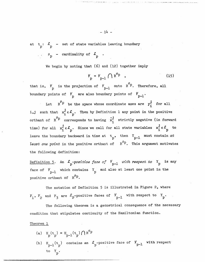
Definition 5. An £ -positive face of Y with respect-to Y is anyp p-1 p
face of Yp-1 which contains Y and also at least one point in the
positive orthant of R P .
The notation of Definition 5 is illustrated in Figure 2, where
F1, F2 and F3 are £p-positive faces of Y-1 with respect to Y .
The following theorem is a geometrical consequence of the necessary
condition that stipulates continuity of the Hamiltonian function.
Theorem 1
(a) H (t) = H (t ) nR 0 Pp p p-1 p
(b) H p l (t ) contains an £ -positive face of Yp-1 with respect
to Yp

- 15 -
Proof:
(a) The Hamiltonian hyperplane H at t isP P
p pH (t ): Z - X )A(t)y? , (16)p p ipix _l
+and the Hamiltonian hyperplane H at t is
p-1 p
+ + J + J (t+)Y ·H p-l(t+): Z= X 'i(t)y+ i(17)
p-' p 1 p 1
Now, Y C H (t-) and Y C H pl (t ) according to the geometric interpreta-
tion. If we now evaluate Hp(t) at any point in Y and Hp l(t+ ) at anyp p P P- p
point in Yp1' the continuity of the Hamiltonian everywhere (equation (2)
of [1) gives
+ - *Z =Z = . (18)
Furthermore, the continuous nature of costates corresponding to state vari-
ables on interior arcs (equation (34) of [1]) gives
xi(t- ) = xi(t) = xJ(t ) Vi,j s.t. Xi £ I (19)ip ip 1I p
By virtue of (18) and (19), we may write the Failtonian hyperplanes
H (t ): Z = XJ(t )y (20)
i Dp p *
Hp l(tp): Z = XJ(t )yJ ,J ('-)
X . 'ii - .
We conclude immnediately from (20) and (21) thai H(tp) Hpl(tp) n R

- 16 -
(b) The argument preceding Definition 5 concludes that Y must
contain at least one point in the positive orthant of R , say yp 1;
therefore y is contained in I (t ). From statement (a) of the
theorem we have that H pl(t ) contains H (t ) and therefore containsp- P P P
Y Consequently, Hp1 (t ) must contain the £ -positive face which
contains both Y and yp -p-l
[I Theorem 1
The geometry associated with Theorem 1 is depicted in Figure 3.
2 i
PP
Figure 3 - Geometry associated with Theorem 1.

- 17 -
III. PROBLEMS OF THE CONSTRUCTIVE DYNAMIC
PROGRAMMING ALGORITHM
The four problems associated with the Constructive Dynamic Program-
ming are now discussed in the light of the geometrical interpretation
developed in the previous section. The order of the presentation of the
problems differs from that in which they appear in the description of the al-
gorithm in Section VI of [1]. In each instance, we first present a brief
statement of the issue as it relates to the algorithm, and afterwards pro-
vide the appropriate geometrical interpretation. The reader is reminded
that attention is being focused on the case in which t p (Tp,tp+l), as
discussed in Section II-C.
A. Leave-the-Boundary Costates
Operation 2 of the algorithm calls for finding those values of the
costate vector at t which satisfy the necessary conditions and allow forp
the optimal departure of £p from the boundary backward in time or for
showing that no such values exist. In detail, given specific values of
xJ(t ), all i,J such that xJ e I , we must find those values of Xj(t1 p 1 p 1 p
all i,J such that x3 evC, so that when maximizing Hpl (tp ) over VY 1
the solution has x3 < 0 for all x C £p, or we must show that no such~i i ~1
values of X3(t ) exist.ip
Geometrically, Theorem 1 says that we essentially want to rotate
H l(t ) around H (t ) by increasing from zero the coefficients X.(t ),p-l p p p ip
all i,j such that xi e£p , until H p l(tp) touches V on an £ -i p p-1p p-l p
positive face with respect to Y . The values of these coefficients at whichp
this condition is achieved constitute a particular set of leave-the-boundary
costates at t provided that they are among the globally optimizing valuesp

- 18 -
for the previous step.l
The rotation is depicted by the arrows in Figure 3. Note that the
rotation is performed while holding time fixed at t (X (t ) for all i,jp i p
such that x? s I do not change) and is to be distinguished from the rota-1 p
tion of the Hamiltonian hyperplane which results from the costates evolving
backward in time.
Suppose that there is more than one such £p-positive face (of various
dimensions < - +p -1) to which H pl(t ) may be rotated in the above
fashion. Then the leave-the-boundary costates achieve those values which
bring H pl(t ) to lie on each of these faces (this is a finitely non-unique
set) and those values which have H pl(t ) lying everywhere between these
faces (this is an infinitely non-unique set). However, the algorithm re-
quires only extreme operating points of V l, that is vertices of Y
for constructing feedback control regions (Operation 4, Section VI of [1]).
Hamiltonian hyperplanes which lie between faces of Vp_1 provide no extreme
operating points in addition to those which lie on the faces. Hence, the
leave-the-boundary costate set at tp can be taken as that finite set cor-
responding to each of the highest dimensional £ -positive faces upon whichp
H l(t ) may be made to lie. See Example 1 of Section IV.
Finally, it may be that there are no appropriate values of X?(t ),zp
all i,j such that xi s.C , which allow Hp (t ) to lie on an £ -posi-' p p-p p
tive face with respect to Y . In that case it is not optimal for £ toP P
leave the boundary backward in time at t .
1. The specification of the globally optimizing values for this step isprovided in Section III-C. This explanation is easily framed in termsof the previous step as required here.
- 19 -
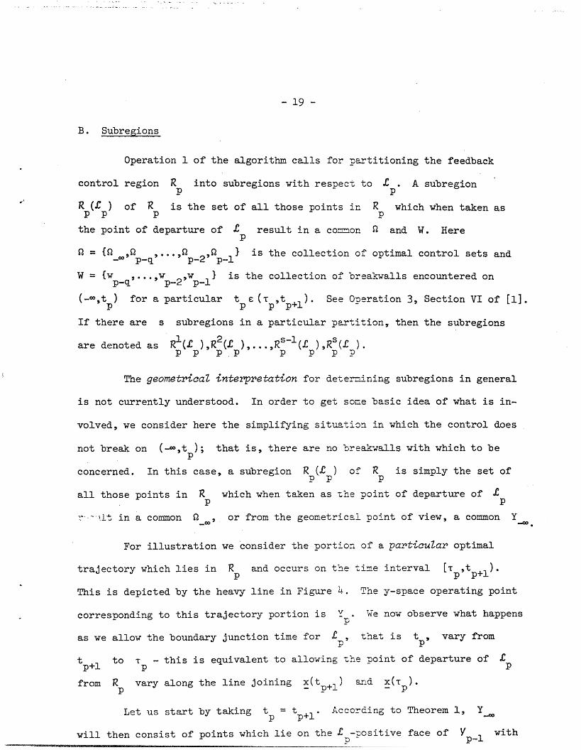
B. Subregions
Operation 1 of the algorithm calls for partitioning the feedback
control region R into subregions with respect to £ . A subregionP P
R (£ ) of R is the set of all those points in R which when taken as
the point of departure of £ result in a co=..on a and W. Herep
=- {2_,p ,_ ... ' p_2, p_1 is the collection of optimal control sets and
W = {w ,...,w ,w I is the collection of breakwalls encountered onp- p-2 p-l
(-at ) for a particular t pe( tp+l ). See 0oeration 3, Section VI of [1].
If there are s subregions in a particular partition, then the subregions
are denoted as R1(C ),R2(£ ),...,RS-1 ( ),RS(. ).pp pp p p P P
The geometrical interpretation for determining subregions in general
is not currently understood. In order to get some basic idea of what is in-
volved, we consider here the simplifying situation in which the control does
not break on (-,t p); that is, there are no breakwalls with which to be
concerned. In this case, a subregion R (£ ) of R is simply the set ofpp p
all those points in R which when taken as the point of departure of £p p
^- u£t in a common Q , or from the geometrical point of view, a common Y
For illustration we consider the portion of a particular optimal
trajectory which lies in RI and occurs on the time interval [T p,t p+l).
This is depicted by the heavy line in Figure 4. The y-space operating point
corresponding to this trajectory portion is Y . We now observe what happens
as we allow the boundary junction time for £p, that is tp, vary from
t +1 to t - this is equivalent to allowing the point of departure of £
from R vary along the line joining x(tp+) and x(T ).
Let us start by taking t = tp+l. According to Theorem 1, Y
will then consist of points which lie on the £ -positive face of Vp 1 withpp

- 20 -
p
p+l
y t R" (- ) P
X(T )
Figure 4- Illustration of subregions of Rp with respect to £p.

- 21 -
respect to Y to which Hp l(t ) may be rotated around H (t ) atP P P
t = t +L For the sake of simplicity we shall assume that Y consists
of exactly one point y'. The corresponding direction in which £ leavesp
R at t = t is indicated by the arrow emanating from the pointp p p+l
x(t +1) in Figure 4.
Now, as tp assumes values continuously backward from tp+l the
solution set Y = y' persists until some time t = T'. At this time thep
set Y_ will change due to the fact that the £p-positive face of Yp-1
with respect to Y upon which Hp l(t ) may be made to lie changes. ThisP p p
is attributable to the fact that H (t ) is rotating as iJ(t ), all i,j
such that x j ¢ I , evolve backward in time. Once again, for simplicity,1 p
assume that the new value of Y is unique and denote it by y". The
corresponding direction with which £ leaves R at t = T' is indicated
by the arrow emanating from the point x(T') in Figure 4.
Assume that the solution set Y = y" persists from T' to T .
Then in this particular situation R consists of two subregions with respect
to £p, R'(C ) and R"(£C ) as indicated in Fizgure 4. The point x(T')p p p p p
lies on a wall separating R'(C ) and R"(C ).pp p p
Knowledge of x(T ') alone is sufficient to determine this wall only
for the case in which Rp is two dimensional - see Example 2 of Section IV
for an illustration of this. For R of arbitrarily high dimension it isp
clear that some correspondingly high number of wrajectories lying in Rp
must be considered from the above point of view, although it is not currently
understood how this may be achieved. Also, since the above discussion is
predicated upon special simplifying assumptions concerning 9, W and Y,
our knowledge concerning the very difficult problem of determining subregions
· ; i ' 'tni 'lete. _.__.._________

- 22 -
C. Global Optimality
Operation 3 of the algorithm for the step under discussion calls for
finding all solutions to the global optimization problem on TE (-,t p)
which satisfy the constraints xJ(T) = 0 for all i,J such that xJ Bi p-l
or show that no such solution exists. In Appendix A of [1l a two-part
approach is suggested for solving this problem:
(a) Find all solutions to the constrained optimization problem.
(b) Produce values of j ( T ) , all i,j such that xj E B and all
rT (-,t ), which satisfy the necessary conditions (15) - (17) of
[1], and such that all solutions to part (a) are also solutions to
the global optimization problem (1) or show that no such values
exist.
As a complete discussion of part (a) is provided in Appendix A of [1],
we concern ourselves here with the solution of part (b).
We begin by specifying those values of Xj (T), all i,j such that1
xisEB and all Te(-o,t ) which satisfy the necessary conditions. Accord-1 p-1 p
ing to equations (15)- (17) of [1], the appropriate costate differential
equations are:
-dX.(T) = a.dT + dn.(T) (22)
dnj?(T) < 0 (23)
Vi,j s.t. x Bp T Ce (,t ) .
If we take T to be time running backward from t , then equations (22)- (23)
indicate that the maximum value that any XJ(T), i,j such that xJ BP
may achieve for a given (t ) is when dT) O. Thereforemay achieve for a given t is whereforei p i

- 23 -
~ <(T) A 'J(t ) + Ad, (24)
Vi,j such that xj B1 p-1
We now provide the geometrical interpretation of part (b), the test
for global optimality of the constrained solution on (-o,tp). First, the
u-space constrained solution sets 2 ,Q ,. p- are globally
optimal if and only if the corresponding y-scace constrained solution sets
Y ,Y ,...,Y 2,Y 1 are globally optimal. We consider the latter sets- p-q p-2' p-l
one at a time beginning with Yp-l1
According to the geometrical interpretation of the constrained opti-
mization problem (Section II-B), Yp-1 is the surface of tangency between
the Hamiltonian hyperplane H (T) of equation (20) and the constraintp-1
figure Y In accordance with the geometrical interpretation of thep-l1
global optimization problem (Section II-A), Y is a global optimum if
and only if there exist values of Ai(-), all i j such that x.sB and allI I p-1
T [Tpltp), which satisfy the necessary conditions and such that the
global Hamiltonian hyperplane H(T) of (3) is tangent to the global con-
straint figure Y at Ypl' The preceding condition holds true for all
T E [Tplt p ) if and only if it holds true for any £ [Frp l,tp). These
observations suggest the following test for global optimality of Y :
Choose any T e [spl,t ). Then Y is a global optimum if and
only if there exist values of X(T) for all ij such that xj1 - ' 1 p-1
which satisfy the necessary conditions anr which cause H(T) to rotate about
H (T) until H(T) becomes tangent to Y av Y 1p-l-1
All values of Xj(9 ), i,j such that xe B , which satisfy the above con-This test is illustrated for
dition constitute the globally optimizing set au z. This test is illustrated for-
- 24 -
a simple situation in Example 3 of Section IV. If Yp-1 is found not to be
a globally optimizing solution, then it is not optimal for the state vari-
ables in £ to leave the boundary. If Y is a global optimum, we nextp p-i
test Y and continue in this fashion until some constrained solution isp-2
shown not to be globally optimum or Y is reached. Feedback control
regions are constructed corresponding to all globally optimal solutions.
D. Off-the-Boundary Assumption
Preceding the description of a step of the algorithm in Section VI
of [1], the following assumption is made, which we call the off-the-boundary
assumption: it is optimal for all of the state variables in Ip-1 to re-
main off the boundary as time runs to minus infinity. This assumption is
implicit in the structure of the Constructive Dynamic Programming Algorithm
since each state variable is allowed to leave the boundary backward in time
exactly once for each optimal trajectory constructed. In principle, the
algorithm can be formulated in the absence of this assumption, but it then
becomes extremely complex.
We now provide the rather simple geometrical interpretation associ-
ated with this assumption:
The off-the-boundary assumption is true for the current step if and
only if there exist constrained solution sets Y ,Yp q...,Yp 2,Yp1 which
all lie in the non-negative orthant of RaP+OP and all of which are global
optima.
This geometrical interpretation is illustrated in Example 4 of
Section IV.

- 25 -
IV. ILLUSTRATIONS OF THE GEOMETRICAL INTERP?3A--0Ni
A. Leave-the-Boundary Costates
Example 1 demonstrates the geometrical interpretation for determin-
ing the leave-the-boundary costates for a situation in which these costates
are non-unique.
Example 1
The general network topology to be considered in this and several
other examples is depicted in Figure 5. The lily capacities are indicated
in brackets, and for simplicity the inputs are -al taken to be zero. The
equations of motion are
2 2 2 2kx(t) -2 (t)- u 3(t) + u3!)
X1 (t) = -u(t) U12(3) 1 1 1 i1cl(t) -u21t) u23(t) + u )2
3 3 3 3i (t) = -u1 3(t) - u 2 (t) +
I 1 1 1~ ~ (25)C(t) =-u 3i(t)- u 3 2 (t) + u23.;
3 3 3 3_x2 (t) -u2 3 (t) -u 2 1 ( t) + U_
x(t) = -u32(t) - u3 1(t) + U1!3 )
1 2 1Let us limit attention now to the state ;ariables x 3 , x 3 and x2
and take the cost functional to be
J = I [x3(t) + x3(t)+ x2(t+- .t
The y-space constraint figure for this problem can readily be obtained by
finding the vertices of U, transforming them i-nt y-space via y = -Bu -a
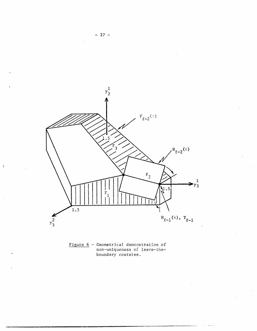
and finally taking the convex hull. The result is presented in Figure 6.

26 -
/2'. x, ,2
X' 1 1 2 s' xu1 u31
Figure 5 - Network topology for Examples 1,5 and 4.
- 27 -
1
Y2
/ ~Vff-2-
1.5
H f2) T Y
Y3
Figure 6 - Geometrical demonstration ofnon-uniqueness of leave-rhe-boundary costates.

- 28 -
We begin by allowing x3 to leave the boundary backward in time at
tf. Since 3(tf) = 0 (Corollary 2 of [1]), and 3(T) = -1 (equation (34)
of [1]), then X3 ( T) > 0 after X3 leaves the boundary backward in time.
Therefore, the zero dimensional Hamiltonian hyperplane Hf (T):f-l
Z = (r)y is minimized over Y at the point Y fl: Y3 = 1.5,
.2 13 = Y2 = 0 as depicted in Figure 6. This solution is of the non-break
variety since it does not change as time approaches minus infinity as long
as no other state variables leave the boundary.
2 1We now allow X3 and x2 to leave the boundary simultaneously at
some arbitrary boundary Junction time tf_ c(-c,t ), that is,~~21~~~~ff f
ff-1 = x3,x2}' . Then according to Definition 5, the £f l-positive faces off-1 332 f21
Yf-2 with respect to Yf-1 are F1, F2 and F3 of Figure 6. Furthermore,
the two dimensional Hamiltonian hyperplane H (t ): Z = X (t )Y3 +f-2 f-l 3 ff- 32 2 1 1
A2(t )y3 + x2(t )y2 can be rotated about the zero dimensional Hamiltonian3 f-1 3 2 f_1 2
hyperplane H (tf) to touch Y in all the faces F l, F2 and F3.f-1 f-l f-2 3
In fact, it may lie on F2 anywhere between F1 and F3. Therefore, the
2 1leave-the-boundary costates A and A at t may achieve values any-3 2 f-l1
where between
t3(t f) = 3 tf =tf tf- 1
{A(tfl) = 0
and
C 2t )=o
jA(t ) tt ) = -t2 (f-l= 3 f- tf-1
Hence, we have an infinitely non-unique set of leave-the-boundary costates
2 1at tf 1 This non-uniqueness persists even after X3 and x2 leave the
boundary backward in time, and enter onto interior arcs.

- 29 -
B. Subregions
We now present an example of the geometricas interpretation applied
to determining subregions. In this case there are two subregions in a par-
ticular two-dimensional feedback control region and the partition into sub-
regions is readily performed.
Example 2
The network is pictured in Figure 7. Once again, for simplicity we
are considering the no-inputs case. This is a single destination network
with all messages intended for node 4; therefore, we may eliminate the
destination superscript on the state and control variables. The dynamical
equations are
xl(t) = u2 1(t)+u 3 1(t)- u (t)
x2(t) = -u2l(t) (26)
x (t)= -u3 (t)
U14 j i [2]
X1
21 U3
X2 37 - Network Topolo
Figure 7 - Network Topology for Example 2
---

- 30 -
and we consider the cost functional
tf
J = f [2x1 (t)+x 2(t)+ 2x3(t)]d t . (27)
The y-constraint figure is depicted in Figure 8.
We begin by letting x2 leave the boundary backward in time at tf.
The constrained optimization problem calls for the maximization of the zero
dimensional Hamiltonian hyperplane Hf_ (T): Z = X2(T)y2 over the constraint
figure f-1 depicted in Figure 8. The costate trajectory for A2 is shown
in Figure 9. The solution to the constrained optimization problem is Yfl:
Y = 0, Y2 = 1.0, y3 = 0. Moreover, it is easy to see by examining Figure 8a
that this solution is globally optimal for the costate values X (T) = 3(T)= 0.
Also, Yf-1 persists as time runs to minus infinity if no other state vari-
ables leave the boundary backward in time. The trajectory is illustrated in
Figure 9. By a simple application of Theorem B.1 of [1], the non-break feed-
back control region Rf_1 may be assigned on the x2-axis as depicted in
Figure 10.
We next stipulate that x3 leaves the boundary at some arbitrary
boundary junction time tf_1 The Hamiltonian hyperplane that touches the
constraint figure Vf_2 in the positive orthant of Y3 is simply H f2(tf_ )
Z = X2 (tf_
1 )y2. Therefore, the leave-the-boundary value of X3 at tf is
zero. As we proceed backward in time from tf 1l' the one-dimensional Hamil-
tonian hyperplane Hf_2(T): Z = X2(T)y2 + X3(T)y3 is maximized over Yf-2
at the point Yf 2: Y1 = 0, Y2 = 1.0, y3 1.0. This solution is globally
optimal for X (T) 0 and does not experience a break as time runs to minus
infinity if no other state variables leave the boundary backward in time. We
construct the two-dimensional non-break feedback control region labled Rf 2
in Figure 10 by once again applying Theorem B.1 of [1].

- 31 -
f-2 f-l y_Y3
1a>I I 1.0
Y~~ /
"~ '~;- YlH \X ~ f- 2H 5 f-l' 1.0 2.0 y
Y25 ~~~fSf-l1 0
Y2
Figure 8 -Geometry for Example 2.(b)
e' Y1~~~~
e Y
H (t )t > Tf-3 f -2 f-2
Y2
(C)~~~~~~~~~~~~~i
-Y~~~~~~Y
f-2~~~~~~~~~-
22
Figure 8 Geometrlv 4or Exam-pie 2.

- 32 -
x
A 2
X 2
A I I I
II7
I \0 >~~t
T f-l tf
Figure 9 - State-costate trajectory pairfor Examole 2.· srrrPP~~~~~~~~~~~~~~~~~~~~~~~~~~~~~~nt~~~~~~~I~aoa~~_ __

- 33 -
x3
j ii~~-2
Rf- 1
Fiure 10 - The subregions R _2(x ) and Rf_2(x) of the
feedback control region 2f-2
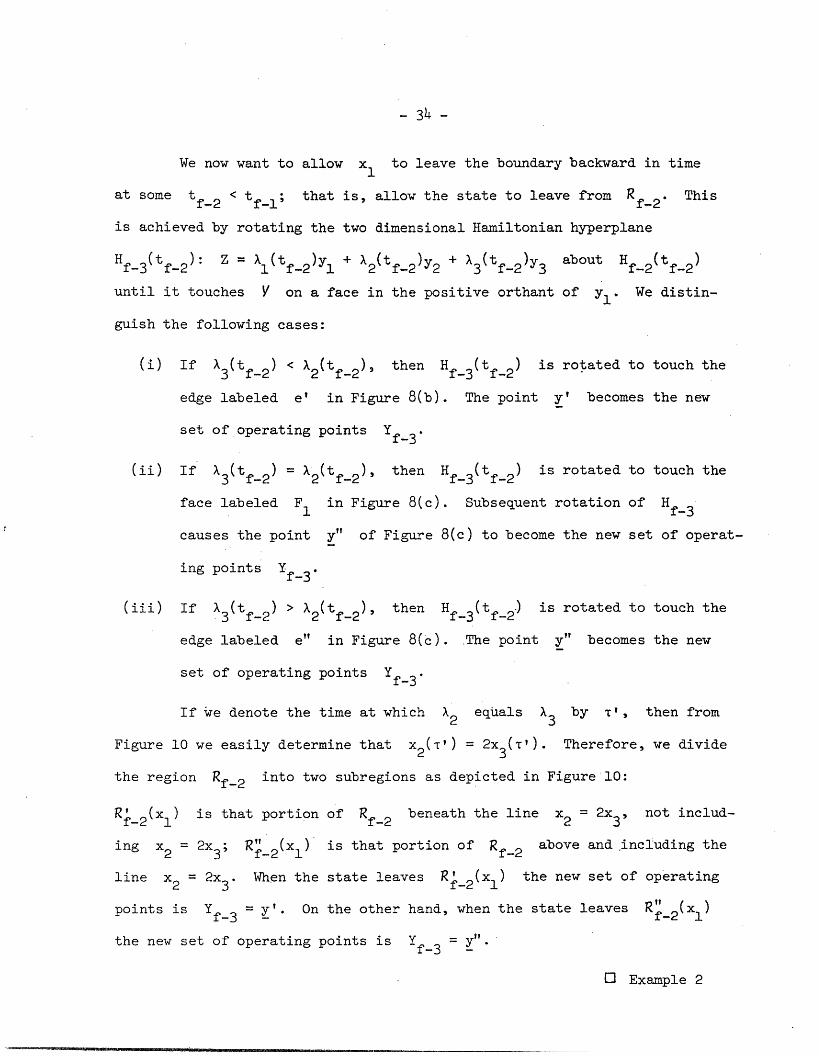
- 34 -
We now want to allow xl to leave the boundary backward in time
at some tf2 < tf; that is, allow the state to leave from Rf2. Thisf-2 f-t f-2_
is achieved by rotating the two dimensional Hamiltonian hyperplane
Hf_3(t _2): Z = 1( f-2)y + 2(tf2)Y2 + A3(tf_2)Y3 about H f_2(tf_2 )
until it touches Y on a face in the positive orthant of yl. We distin-
guish the following cases:
(i) If (tf_2) < 2(t f_2), then H (tf) is rotated to touch the
edge labeled e' in Figure 8(b). The point y' becomes the new
set of operating points Yf_3.
(ii) If A3(tf 2) = 2 (tf_2 ), then Hf 3(tf 2 ) is rotated to touch the
face labeled F1 in Figure 8(c). Subsequent rotation of Hf-3
causes the point y" of Figure 8(c) to become the new set of operat-
ing points Yf-3'
(iii) If A3(tf_2) > A2(tf_2) then Hf 3(tf 2) is rotated to touch the
edge labeled e" in Figure 8 (c). The point y" becomes the new
set of operating points Yf-3'
If we denote the time at which A2 equals A3 by -', then from
Figure 10 we easily determine that x2(T' ) = 2x3(T'). Therefore, we divide
the region Rf_2 into two subregions as depicted in Figure 10:
RI 2(x1) is that portion of Rf_2 beneath the line x2= 2x3, not includ-
ing x2 = 2x3; R t 2(x1) is that portion of Rf_2 above and including the
line x2 2x3 . When the state leaves R _2(x1 ) the new set of operating
points is Y = y'. On the other hand, when the state leaves Rf 2(xC)f-3 f-2x1
the new set of operating points is Yf-3 = y".
0 Example 2

- 35 -
C. Global Optimality
A simple example is now presented to illustrate the geometrical
interpretation for determining if a solution to the constrained optimiza-
tion problem is globally optimal. In the particular situation presented,
global optimality does not hold.
Example 3
Once again consider the network topology of Figure 5.
For the purpose of this example, we limit attention to the state
1 1variables X3 and x2 and consider the cost function
3
to
We begin by letting xl leave the boundary backward in time at tf.ff
Then the constrained optimization problem in y-space calls for the maximiza-
tion of the zero dimensional Hamiltonian hyperlne H ): Z (28)Yf-l 2 2
over the constraint region Y depicted in Fiogre 11. The trajectoryf-l
for Xi is shown in Figure 12. The solution to the constrained optimiza-2
1 1tion problem is Y f-1: Y2
= 1.5, y3 = 0, as illustrated in Figure 11.
Now, for any T < tf let us see if there exists some value of 3(T) such
that the global Hamiltonian hyperplane H(T): Z = X (T)y I + (T)y is2 2 3 3
tangent to V at Yf-l' From Figure 11 it is seen that the only possible
such value is AX (T) = A(T). However, from (24) and the transversality3 2
condition (equations (19) of [1]) we have 3 (T) < - A (T) as depicted in3 -2 2
Figure 12. Therefore, the candidate operating point Yf-1 obtained from
the constrained optimization is not a global optimum.
1 Example 3.
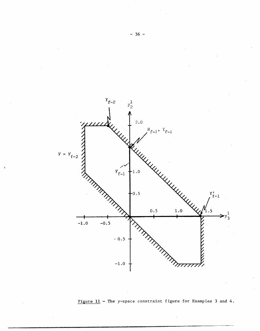
- 36 -
Yf-2 1Y2
~fJ-2 ~ ~ ~
f-I 0.5 1.0
y 3
-- 0.5
-1.0
Figure 11 - The y-space constraint figure for Examples 3 and 4.

- 37 -
I ~-2
tt
Figure 12 - Costate Trajectories 2r Example 3.
D. Off-the Boundary Assumption
Example 4 demonstrates the geometvrical interpretation for testing
the validity of the off-the-boundary assulrption for a situation in which the
assumption does not hold.
Exam-Ple 4
We once again refer to the network topoc^E_, of Figure 5 and concern
ourselves with the state variable x2 and x as in Example 3. The y-space
constraint figure appears as in Figure 11, and the cost functional is taken
as (28).

- 38 -
In example 3, we attempted to allow x2 to leave the-boundary back-
ward in time at tf and discovered that such a trajectory cannot be globally
optimal. We now try letting x3 leave the boundary backward in time at tf.
The trajectory for X is shown in Figure 13 and the non-break solution to
1the constrained optimization problem is readily seen to be Y' Y2 =
f-l 21 1y 1.5 from Figure 11. This solution is globally optimal when A2(T) is
taken to be equal to X (T). This value of X (T) satisfies (24) with3 2
equality since the transversality condition requires (tf) = 0.
Suppose we now allow x2 to leave the boundary backward in time at
the arbitrary boundary junction time tf_1 < tf. It is readily seen that the
leave-the-boundary value of X (t ) is achieved when it is equal to2 f-l
X (tf). Once x2 leaves the boundary backward in time its costate travels3 f-l 2
as indicated in Figure 13. Since X 1 (T) > lA(T) for T < tf , then the2 3 f-l
only globally optimizing operating point in this situation is Yf-2:
1 1Y2
= 2.0, y3 = -0.5. Hence, the optimal slope of x3 forward in time is
+0.5 and therefore x3 must return to the boundary backward in time.
[ Example 4

- 39 -
1
3 = 2-1 < 2
tf 1 tf
Figure 13 - Costate trajectories for Example 4.
- 40 -
V. DISCUSSION AND CONCLUSIONS
In this paper a geometrical interpretation has been presented which
provides the principles for coping with the problems of the Constructive
Dynamic Programming Algorithm listed in Section VI of [1]. However, it is
not currently known how this approach may be applied to construct a numerical
version of the algorithm for general network problems. The fundamental com-
plication is that the geometrical interpretation requires explicit knowledge
of the y-space constraint figure and although we may readily find the appro-
priate constraints for simple cases of three dimensions or less (as in
Examples 1-4), it is not understood how this may be accomplished for problems
of arbitrarily high dimension.
Another complication is that it is desirable to determine the
validity of the "off-the-boundary assumption" a priori for all possible
optimal trajectories corresponding to a given network problem. Whether or
not this assumption holds for a given problem is a basic property which
determines the applicability of the Constructive Dynamic Programming Algorithm.
No technique is currently known for the a priori assessment of the validity
of this assumption for general network problems.
Nonetheless, the geometrical interpretation presents several signifi-
cant benefits. To begin it provides a powerful conceptual tool for gaining
insight into the necessary conditions of optimality associated with continuous
linear optimal control problems with linear state and control variable
inequality constraints. The insight which is gained may be of interest
exclusive of its applicability to the Constructive Dynamic Programming Algor-
ithm itself. For example, we have formulated a compact geometrical condition
for determining the uniqueness or nonuniqueness of the costate variables, and

- 41 -
have used it to demonstrate the potential non-,ircsqueness of costate variables
at times when their corresponding state variables are travelling on interior
arcs (Example 1). This is a most interesting property which characterizes
linear state constrained optimal control problems. Although it is well known
that nonuniqueness of the costate variables may occur in nonlinear state
constrained optimal control problems (see for example [3] and [4]), it is
limited to those costate variables corresoondi-rn to state variables travel-
ling on boundary arcs or at boundary junctions.
From the point of view of Constructive D,--mic Programming Algorithm,
the geometrical interpretation provides the theoretical framework for recogniz-
ing and proving simplifications which arise i- stecial network problems. In
a forthcoming paper by the authors (Part III of tnis series) the geometrical
interpretation is applied to the case of single destination networks with
all unity weightings in the cost functional to prove several simplifications
which permit a numerical formulation of the Cons-Vtactive Dynamic Programming
Algorithm for that problem. Briefly, these sim--fications are:
1. Uniqueness of the leave-the-boundary cosyates.
2. Exactly one subregion per every feedbac-k control region.
3. Solutions to the constrained optimizat--on problems are always
globally optimal.
4. An optimal control always exists withscu breakpoints between
boundary junctions.

- 42 -
References
[1] Moss, F.H. and Segall, A., "An Optimal Control Approach to DynamicRouting in Data Communication Networks, Part I: Principles",submitted to IEEE Trans. Autom. Control.
[2] Segall, A., "The Modelling of Adaptive Routing in Data-CommunicationNetworks", IEEE Trans. Comm., Vol. COM-25, No. 1, pp. 85-95,
January 1977.
[3] Bryson, A.E., Denham, W.F. and Dreyfus, S.E., "Optimal ProgrammingProblems with Inequality Constraints I: Necessary Conditionsfor Extremal Solutions", AIAA J. 1, No. 11, 2544-2550, 1963.
[4] Jacobson, D.H., Lele, M.M. and Speyer, J.L., "New Necessary Conditions
of Optimality for Control Problems with State-VariableInequality Constraints", J. of Math. Anal. and AppZ., Vol. 35,No. 2, 255-284, August 1971.