Embed Size (px)
Citation preview
Kaisa Peltoniemi
Improving Purchasing by Inventory Management
Inventory Management in Spare Part Business
Helsinki Metropolia University of Applied Sciences
Master of Business Administration
Supply Chain Management
Master’s Thesis
Date 10.8.2018
Abstract
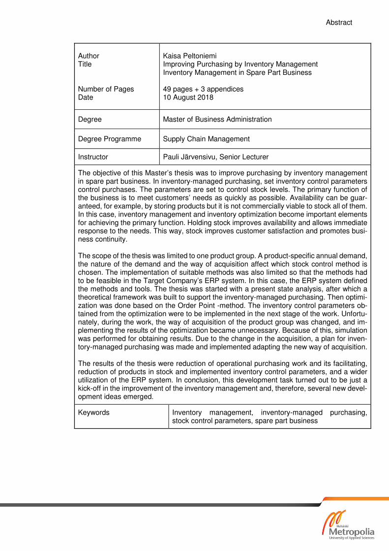
Author Title Number of Pages Date
Kaisa Peltoniemi Improving Purchasing by Inventory Management Inventory Management in Spare Part Business 49 pages + 3 appendices 10 August 2018
Degree Master of Business Administration
Degree Programme Supply Chain Management
Instructor Pauli Järvensivu, Senior Lecturer
The objective of this Master’s thesis was to improve purchasing by inventory management in spare part business. In inventory-managed purchasing, set inventory control parameters control purchases. The parameters are set to control stock levels. The primary function of the business is to meet customers’ needs as quickly as possible. Availability can be guar-anteed, for example, by storing products but it is not commercially viable to stock all of them. In this case, inventory management and inventory optimization become important elements for achieving the primary function. Holding stock improves availability and allows immediate response to the needs. This way, stock improves customer satisfaction and promotes busi-ness continuity. The scope of the thesis was limited to one product group. A product-specific annual demand, the nature of the demand and the way of acquisition affect which stock control method is chosen. The implementation of suitable methods was also limited so that the methods had to be feasible in the Target Company’s ERP system. In this case, the ERP system defined the methods and tools. The thesis was started with a present state analysis, after which a theoretical framework was built to support the inventory-managed purchasing. Then optimi-zation was done based on the Order Point -method. The inventory control parameters ob-tained from the optimization were to be implemented in the next stage of the work. Unfortu-nately, during the work, the way of acquisition of the product group was changed, and im-plementing the results of the optimization became unnecessary. Because of this, simulation was performed for obtaining results. Due to the change in the acquisition, a plan for inven-tory-managed purchasing was made and implemented adapting the new way of acquisition. The results of the thesis were reduction of operational purchasing work and its facilitating, reduction of products in stock and implemented inventory control parameters, and a wider utilization of the ERP system. In conclusion, this development task turned out to be just a kick-off in the improvement of the inventory management and, therefore, several new devel-opment ideas emerged.
Keywords Inventory management, inventory-managed purchasing, stock control parameters, spare part business
Tiivistelmä
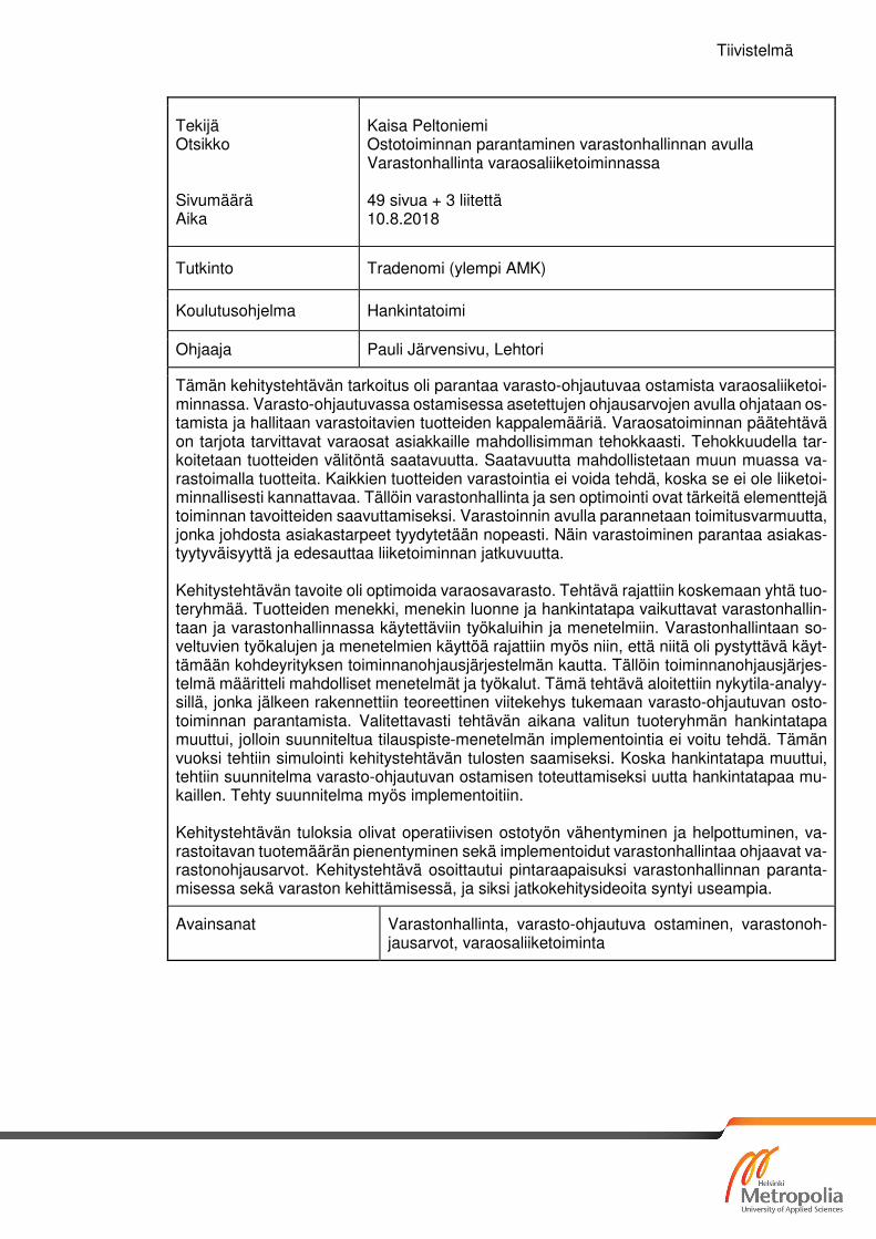
Tekijä Otsikko Sivumäärä Aika
Kaisa Peltoniemi Ostotoiminnan parantaminen varastonhallinnan avulla Varastonhallinta varaosaliiketoiminnassa 49 sivua + 3 liitettä 10.8.2018
Tutkinto Tradenomi (ylempi AMK)
Koulutusohjelma Hankintatoimi
Ohjaaja Pauli Järvensivu, Lehtori
Tämän kehitystehtävän tarkoitus oli parantaa varasto-ohjautuvaa ostamista varaosaliiketoi-minnassa. Varasto-ohjautuvassa ostamisessa asetettujen ohjausarvojen avulla ohjataan os-tamista ja hallitaan varastoitavien tuotteiden kappalemääriä. Varaosatoiminnan päätehtävä on tarjota tarvittavat varaosat asiakkaille mahdollisimman tehokkaasti. Tehokkuudella tar-koitetaan tuotteiden välitöntä saatavuutta. Saatavuutta mahdollistetaan muun muassa va-rastoimalla tuotteita. Kaikkien tuotteiden varastointia ei voida tehdä, koska se ei ole liiketoi-minnallisesti kannattavaa. Tällöin varastonhallinta ja sen optimointi ovat tärkeitä elementtejä toiminnan tavoitteiden saavuttamiseksi. Varastoinnin avulla parannetaan toimitusvarmuutta, jonka johdosta asiakastarpeet tyydytetään nopeasti. Näin varastoiminen parantaa asiakas-tyytyväisyyttä ja edesauttaa liiketoiminnan jatkuvuutta. Kehitystehtävän tavoite oli optimoida varaosavarasto. Tehtävä rajattiin koskemaan yhtä tuo-teryhmää. Tuotteiden menekki, menekin luonne ja hankintatapa vaikuttavat varastonhallin-taan ja varastonhallinnassa käytettäviin työkaluihin ja menetelmiin. Varastonhallintaan so-veltuvien työkalujen ja menetelmien käyttöä rajattiin myös niin, että niitä oli pystyttävä käyt-tämään kohdeyrityksen toiminnanohjausjärjestelmän kautta. Tällöin toiminnanohjausjärjes-telmä määritteli mahdolliset menetelmät ja työkalut. Tämä tehtävä aloitettiin nykytila-analyy-sillä, jonka jälkeen rakennettiin teoreettinen viitekehys tukemaan varasto-ohjautuvan osto-toiminnan parantamista. Valitettavasti tehtävän aikana valitun tuoteryhmän hankintatapa muuttui, jolloin suunniteltua tilauspiste-menetelmän implementointia ei voitu tehdä. Tämän vuoksi tehtiin simulointi kehitystehtävän tulosten saamiseksi. Koska hankintatapa muuttui, tehtiin suunnitelma varasto-ohjautuvan ostamisen toteuttamiseksi uutta hankintatapaa mu-kaillen. Tehty suunnitelma myös implementoitiin. Kehitystehtävän tuloksia olivat operatiivisen ostotyön vähentyminen ja helpottuminen, va-rastoitavan tuotemäärän pienentyminen sekä implementoidut varastonhallintaa ohjaavat va-rastonohjausarvot. Kehitystehtävä osoittautui pintaraapaisuksi varastonhallinnan paranta-misessa sekä varaston kehittämisessä, ja siksi jatkokehitysideoita syntyi useampia.
Avainsanat Varastonhallinta, varasto-ohjautuva ostaminen, varastonoh-jausarvot, varaosaliiketoiminta
Contents
1 Introduction 1
2 Glossary 3
3 Master’s Thesis for a Target Company 4
3.1 Scope of the thesis 5
3.1.1 Validity, Reliability and Verification 7
4 Present State Analysis 8
4.1 Inventory 8
4.2 Purchasing 13
5 Towards a Successful Inventory Management 17
5.1 Inventory turnover 18
5.2 Stock profile figure 18
5.3 Inventory control methods 19
5.3.1 Safety stock 19
5.3.2 Order point 21
5.3.3 Min-Max 22
5.3.4 Right amount, proper time 22
5.3.5 Scrap the dead stock 23
5.4 Classification 24
5.4.1 Forecasting 25
6 Optimizing & Implementing 27
6.1 Product group and goals for optimization 27
6.2 Inventory availability planning 28
6.3 Visualizing 29
6.4 Simulating Order point -method 31
6.4.1 Orange 33
6.4.2 Yellow and Blue 34
6.4.3 Green 36
6.4.4 Results 37
6.5 Adapting the new way of acquisition 40
6.5.1 Results 42
6.6 Conclusions 43
6.6.1 Ideas for future development 45
References 48
Appendices
Appendix 1. Object and goal (not published)
Appendix 2. Visualized profiles and discussions
Appendix 3. Safety stocks, orders points and amounts
1
1 Introduction
“Supply chain management (SCM) is the management of a network of interconnected
businesses involved in the ultimate provision of product and service packages required
by end customer. SCM spans all movement and storage of raw materials, work-in-pro-
cess inventory, and finished goods from point of origin of consumption” (Samson 2011,
ix).
This Master’s thesis was performed to achieve a more effective supply chain in spare
parts business. The aims of the thesis were to make more use of existing enterprise
resource planning system (ERP) in inventory management and to decrease workload
due to operative purchasing when appropriate. ERP tools were especially needed for
inventory management purposes; demand forecasting, inventory availability planning
and automation of purchasing. This Master’s thesis deals with inventory-managed pur-
chasing from a viewpoint of a separately chosen, specified product group.
In the Target Company’s spare parts business was increasing need to develop purchas-
ing activities for the growing business. The activities were handled by a purchaser,
whose full-time working hours were not enough to handle all the work. The purchaser is
responsible for operational purchasing; ordering, order monitoring and invoice handling,
supplier relations; cooperation and development of the relation, product data updates;
possible new suppliers, bidding activities and sales product pricing, and availability of
sales products; inventory management. In the purchaser’s point of view, an instant need
was to analyze and rationalize existing stock and to automate operative purchasing by
the ERP tools as much as possible. Using the ERP system more widely, the system
could provide information for optimizing the entire inventory. By these changes, the pur-
chaser could be capable to focus on proactive purchasing instead of reactive purchasing.
There were questions in four different sub targets that needed to be answered. Firstly,
what are the potentialities of existing ERP system to provide forecasting of demand, to
optimize stock levels and to define stock keeping units (SKU), to analyse inventory turn-
over ratios and to automate purchases? What kinds of ERP tools are existing, how to set
up and use them? Secondly, there is a large number of products and no actual high-
volume products in the business, how to predict the need and to plan stock availability in
2
an intermittent and lumpy demand where customer’s need is now or sooner and the
number of spare part products is huge? Thirdly, what are the products and product clas-
ses that are reasonable for the business to dedicate resources? In what kind of catego-
ries the products should be divided into? And finally, the business is measured using
three key performance indicators (KPI), but purchasing functions are not measured.
What are suitable indicators for purchasing and what are the benefits of measuring it in
this particular business?
At the beginning of the research it became very clear that all the set sub targets cannot
be solved within this research. Simply too many issues to study and solve in a short time.
Because of this, the aims and objectives were limited to following subjects:
1. studying inventory-managed purchasing and studying methods for stock
control
2. studying Target Company’s ERP’s planning tool for a successful inventory
management
3. Implementing the learned knowledge to a separately chosen, specific prod-
uct group if reasonable and clarifying the needs for future development.
This development work was performed by an action research. The first step was to ana-
lyse the present state. After that, the appropriate theory was investigated and studied.
Together with the Target Company’s business management, the directions for the de-
velopment as well as desired goals were found and accepted.
In the beginning of 2018 the business management decided to change the way of acqui-
sition of the specified product group. At this point the optimization was already done and
the implementation was supposed to be performed. Because of the change, the imple-
mentation could be performed only partly. The implementation was done on March 2018.
There was no time to go back to the drawing board, so the simulation of 2017 was per-
formed to get the results. The simulation was performed on April 2018. The simulation
should have been performed anyway to evidence the effect of the changes that had been
done, since the results of the implementation would not have been visible during this
action research.
Because of the change, a plan for inventory-managed purchasing that adapts a new way
of acquisition was made on April 2018. Some results could be derived from the plan and
are presented in this paper.
3
2 Glossary
ERP, refers to a company-wide information
Enterprise resource planning system for managing the company’s opera-
tional and support processes (Weele 2014, 256)
EOQ economical order quantity
Inventory turnover measures economic efficiency of inventory
control of meeting demand
(Baily etc. 2005, 142)
KPI, are derived from a company’s strategy. The
Key performance indicators course of an action and the achievement of
goals are measured by set key performance in-
dicators
MRP, is a tool for purchasing and inventory planning
Materials requirements planning which determines a need of materials
Q1-4, quarter of a year. Q1 is January-March,
Quarter 1-4 Q2 is May-June, Q3 is July-September and Q4
is October-December
Spare part business one of the Target Company’s business units
which is managed by the Service department
Service level measures success in meeting demand off the
self (Baily etc. 2005, 142)
SKU, Stock keeping unit is a unit in stock
Target Company a company for which the thesis is performed for
4
3 Master’s Thesis for a Target Company
A company’s development work is usually performed to achieve new or more effective
practice, function or way of working. Development work is performed also for creating or
developing products or services based on the environment the company is performing
at and for the needs of the company. (Ojasalo, Moilanen & Ritalahti 2015, 11)
This Master’s thesis is a development work performed for a target company and per-
formed as an action research. The purpose of the action research is to investigate, ana-
lyze, develop, implement and summarize knowledge for the target company’s needs.
(Masters 2018, 4 and 11)
It is very important to understand that continuous development is a key factor for com-
pany’s success. By continuous development the company is capable to respond to future
demand and make plans for the future in a variable environment. Digitalization and glob-
alization create needs for changes in companies’ operations. The global knowledge is
increasing all the time. It means that companies’ operations are based more and more
to knowledge and its management. It is crucial to find, study and understand the precise
knowledge from the mass of data that serves the company’s needs. At the same time
the speed of changes is increasing and predicting the future becomes more complicated.
Company’s success depends on how capable the company is for transformation and
how flexible the company’s operations are for changes. The company’s ability to inno-
vate, for example customer-driven innovations, enables company success in the future.
(Ojasalo etc. 2015, 12-14)
An action research is considered as one of the qualitative research methodologies. The
qualitative research aims at deep understanding of a phenomenon. It is a flexible re-
search methodology that can be proceeded and performed according to the prevailing
situation. During the qualitative research, new hypotheses are created. Qualitative anal-
ysis is a cyclical process. The analysis is a continuous activity that goes on through the
research. The analysis guides the research process and data collection. In a qualitative
research process, analysis and data collection alternate. (Kananen 2014, 20-23)
One element of the action research is a permanent change. This way the action research
gives a promise for a better future. This can also be seen as a democratic activity that
begins with those that it concerns and their own power to find a solution for the issue.
The action research is a continuous improvement of operations. (Kananen 2014, 11)
5
The action research requires scientific and social debate of the field the research is as-
sociated with. The research’s performer must be an expert with a large knowledge of
different research methods. This is how the action research differs from a functional the-
sis. In the functional thesis the performer is a student who is emerging as an expert and
the scientific and social debate is not demanded. (Vilkka 2006. 76-77)
3.1 Scope of the thesis
The objects of this action research were the Target Company’s spare parts stock and
spare parts purchasing. The main targets in this action research were to explore suitable
ways to perform
• inventory management in spare part business
• purchasing that decreases work load in operative purchasing
The purpose was to reduce the amount of operative work in purchasing by migrating
from order-managed to inventory-managed purchasing. The idea was to study the op-
portunities of inventory-managed purchasing. These opportunities had to be suitable to
be executed with the Target Company’s ERP and had to follow the Target Company’s
goals. Therefore, the first steps were to clarify the goals for the inventory management
and to explore existing inventory management opportunities from the ERP. In this action
research the migration was not performed nor implemented.
The purpose was not to get rid of order-managed purchasing, but to develop purchasing
function, where appropriate, to inventory-managed direction. This aims at managing the
products in stock by product classes. In this action research the product classification
has not been performed nor implemented, but the classification has briefly discussed
because it is heavily associated with the inventory management and is related to the
future development.
According to my opinion and experience, the inventory management seeks to obtain an
optimized state of a stock. This means a stock state which is serving the Target Com-
pany’s business in the best possible way. The more efficient the inventory management
and the purchasing activities are, the better the customer satisfaction will be, and the
continuity of the business is ensured. After all, it is always about customer satisfaction.
The speed and punctuality of customer order deliveries are increasingly affecting the
6
decision of where the customers are ordering the products (Salmivuori 2010, 7). In the
Target Company’s spare part business, the availability plays a very big role, because
usually the customers enquire spare parts when the actual need prevails. It means that
the business must be able to respond to the need as rapidly as possible. Without stocks
and accurate management, it cannot be done. However, this doesn’t mean that the
stock needs to be located in own premises or in own accountancy.
In this action research the optimization for the entire spare part stock and all its products
was not possible to be performed. Therefore, a specific product group (chapter 3.1.1)
was chosen to be studied and optimized. This action research deals the inventory-
managed purchasing from a viewpoint of chosen product group.
Achievements of the action research were expected to be
• optimized product-specific stock control parameters implemented in the
ERP to control the stock levels and purchases
• knowledge of using ERP’s Inventory part planning tool
• ideas for further development
The achievements of this action research were measured with the following met-
rics (1-4).
1. Customer service; late deliveries in 2017 compared to late deliveries in sim-
ulation. Delivery gets the status “late” if it’s not delivered from stock.
2. Inventory turnover; the change between non-optimized and optimized. In
inventory management, the turnover rate indicates the efficiency in rota-
tion. The higher the rate the better the rotation. (Chapter 5.1)
3. Average yearly inventory value (%); the difference between non-optimized
and optimized inventory values.
4. Work load (%); percentage difference between time spent per purchase or-
der line in 2017 and time spent per purchase order line in optimization.
7
3.1.1 Validity, Reliability and Verification
The output data for this action research was gathered from the Target Company’s ERP
system. The data accuracy is controlled by annual audits based on existing quality stand-
ards to which the Target Company is committed. User authorizations are limited to spe-
cific profiles according to the job description. The data in the system is unchangeable
unless someone purposely changes it. In case of a change, the person behind the
change can be pointed out and made change can be questioned. A manually made
change always leaves a mark in the system.
The Target Company’s ERP system limited the use of potential theories because the
developmental change was to be feasible in the ERP system. The theories used in this
action research are valid in this specific intended use. The theoretical framework was
investigated and built to support the scope of this action research. It goes without saying
that all the world's theories were not studied but appropriate theories were widely inves-
tigated. Used theories were derived from several sources and the found sources sup-
ported each other. The theories were chosen so that they were applicable to the devel-
opment tasks and responded to its demands and research questions. The theories men-
tioned in this action research are commonly and well known in literature on supply chain
management, inventory management, logistics, purchasing, etc.
The data used in this action research can be repeatedly gathered from the ERP system.
Output data was heavily processed during the research but all the actions done are doc-
umented and archived, and can be verified. Unpredictable changes in business environ-
ment as well as strategic changes done by the business management can affect the
verification and validity of this research. However, there are no remarkable changes ex-
pected in the near future. As mentioned before, the research is performed for the partic-
ular product group in this particular business environment.
8
4 Present State Analysis
This chapter discusses about the present state of a stock, and its functions and manage-
ment. The stock belongs to the Target Company’s Service department’s (Service) Spare
part business, and is part of the Target Company’s Inventory. In order to obtain a better
overall view of the present state, a stock and its functions under Project department
(Project) may be briefly introduced and discussed. This chapter is written from a Ser-
vice’s purchaser‘s point of view.
4.1 Inventory
This inventory present state analysis was made based on the inventory levels on
27.10.2017 unless otherwise advised. Output data was collected from the ERP system.
The ERP query was made using the criteria: all inventory parts in stock with on-hand
quantity more than zero. The result was
• 3 818 different products and
• 113 815 pieces of product units in the Inventory.
The Inventory contains all inventory parts with on-hand quantity more than zero, without
considering the stock location. For example,
• Part A: on-hand quantity is three pieces and is stocked at supplier’s premises
and
• Part B: on-hand quantity is one piece and is stocked at the Inventory.
According to the above, all the 113 815 pieces of product units are not at the same
location nor in the Inventory.
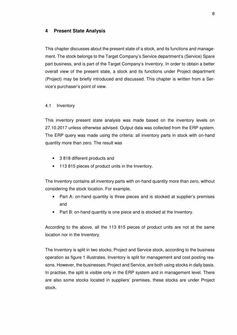
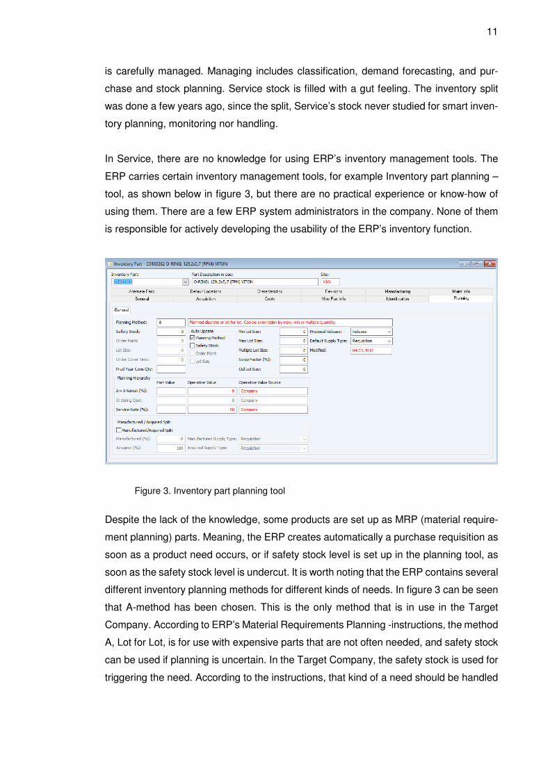
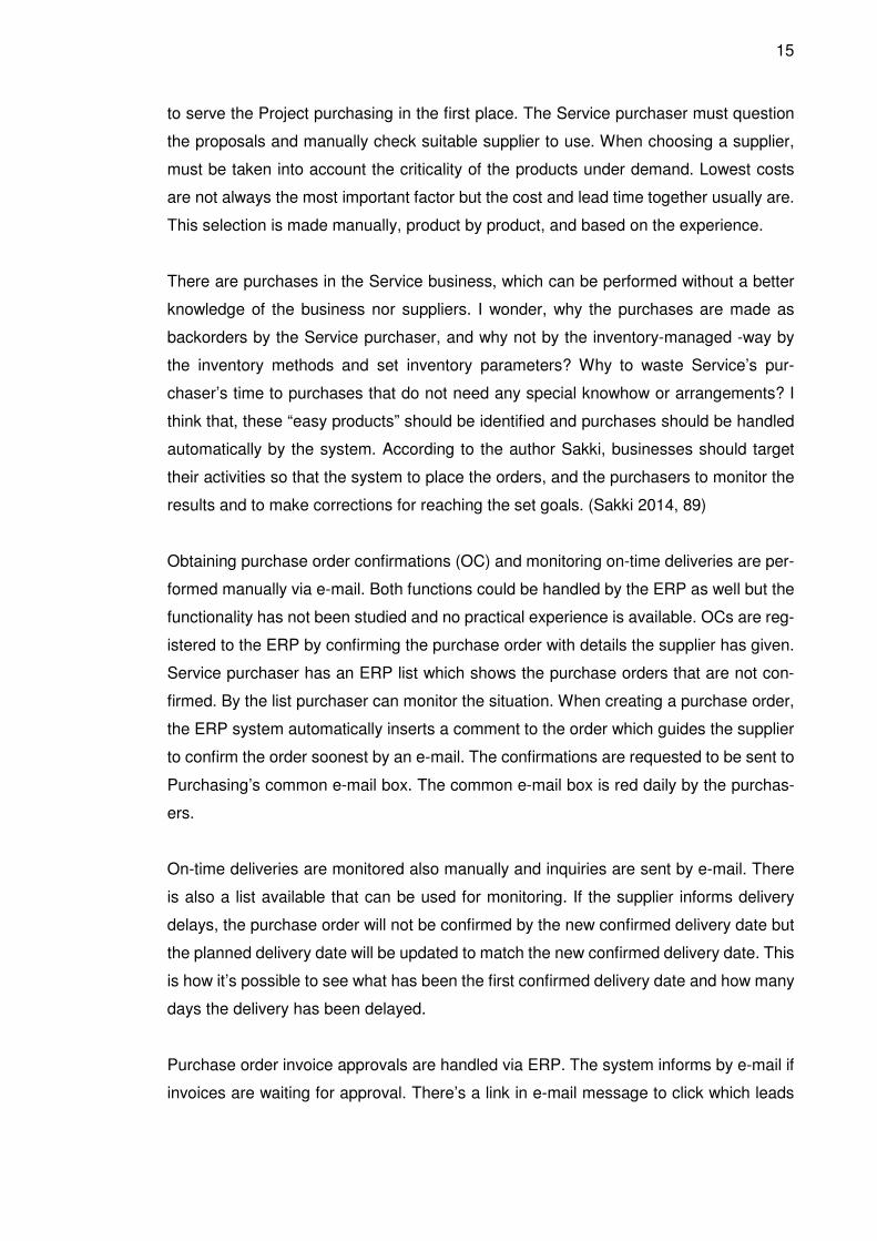
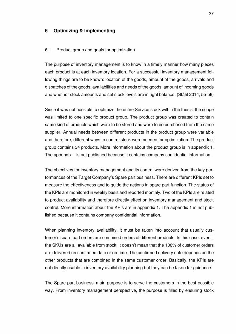
The Inventory is split in two stocks; Project and Service stock, according to the business
operation as figure 1 illustrates. Inventory is split for management and cost posting rea-
sons. However, the businesses; Project and Service, are both using stocks in daily basis.
In practise, the split is visible only in the ERP system and in management level. There
are also some stocks located in suppliers’ premises, these stocks are under Project
stock.
9
Figure 1. Inventory split; Service and Project, 27.10.2017
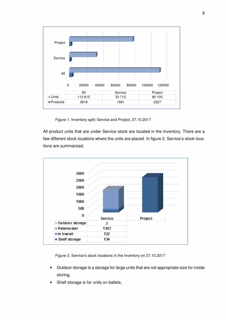
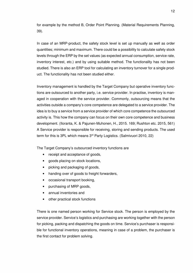
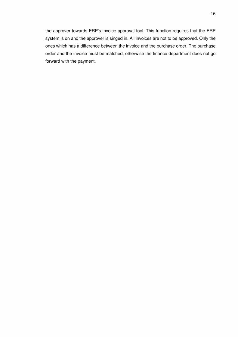
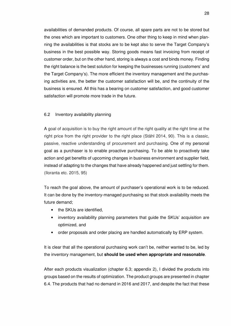
All product units that are under Service stock are located in the Inventory. There are a
few different stock locations where the units are placed. In figure 2. Service’s stock loca-
tions are summarized.
Figure 2. Service’s stock locations in the Inventory on 27.10.2017
• Outdoor storage is a storage for large units that are not appropriate size for inside
storing,
• Shelf storage is for units on ballets,
0 20000 40000 60000 80000 100000 120000
All
Service
Project
All Service Project
Units 113 815 33 712 80 103
Products 3818 1591 2227
10
• Paternoster is a vertical carousel storage (Rushton etc. 2015, 293-294) where
small units are stocked. The Paternoster is a primary storage, all units that are
appropriate size are stock there,
• Storage called “In transit” is for units that are purchased for a customer order and
received in the Inventory. Units are In transit -storage until customer order pick-
ing, before customer order delivery.
There was 1 591 pieces of different products and 33 712 pieces of product units in Ser-
vice stock. Based on my calculations, 20% of products holds a bit less than 83% of total
stock value and 10% of products holds 70% of total stock value.
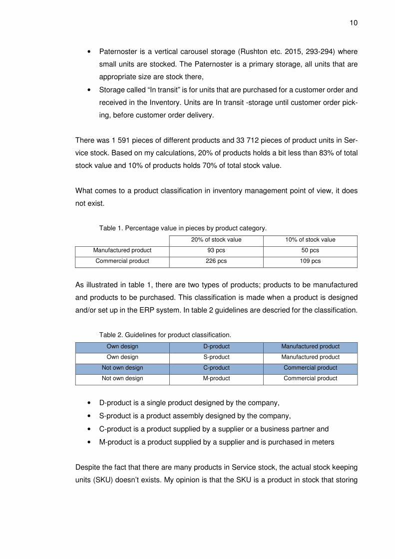
What comes to a product classification in inventory management point of view, it does
not exist.
Table 1. Percentage value in pieces by product category.
20% of stock value 10% of stock value
Manufactured product 93 pcs 50 pcs
Commercial product 226 pcs 109 pcs
As illustrated in table 1, there are two types of products; products to be manufactured
and products to be purchased. This classification is made when a product is designed
and/or set up in the ERP system. In table 2 guidelines are descried for the classification.
Table 2. Guidelines for product classification.
Own design D-product Manufactured product
Own design S-product Manufactured product
Not own design C-product Commercial product
Not own design M-product Commercial product
• D-product is a single product designed by the company,
• S-product is a product assembly designed by the company,
• C-product is a product supplied by a supplier or a business partner and
• M-product is a product supplied by a supplier and is purchased in meters
Despite the fact that there are many products in Service stock, the actual stock keeping
units (SKU) doesn’t exists. My opinion is that the SKU is a product in stock that storing
11
is carefully managed. Managing includes classification, demand forecasting, and pur-
chase and stock planning. Service stock is filled with a gut feeling. The inventory split
was done a few years ago, since the split, Service’s stock never studied for smart inven-
tory planning, monitoring nor handling.
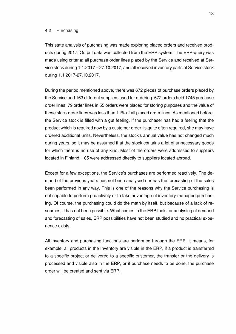
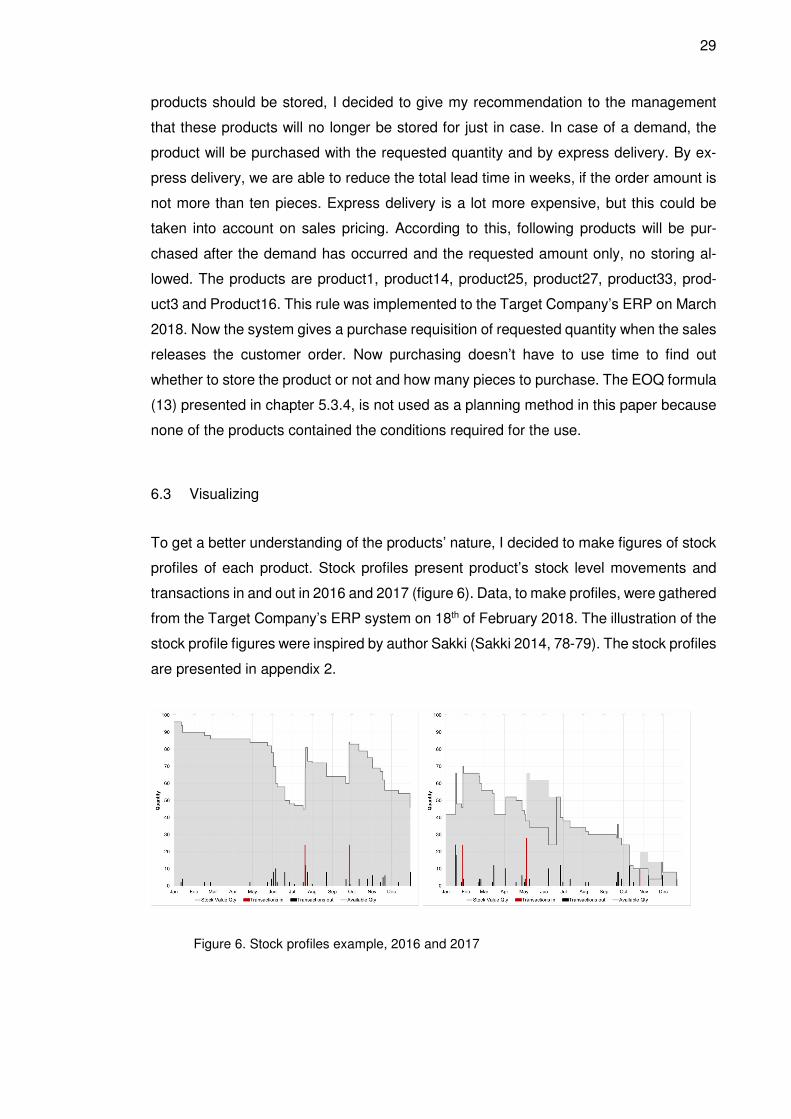
In Service, there are no knowledge for using ERP’s inventory management tools. The
ERP carries certain inventory management tools, for example Inventory part planning –
tool, as shown below in figure 3, but there are no practical experience or know-how of
using them. There are a few ERP system administrators in the company. None of them
is responsible for actively developing the usability of the ERP’s inventory function.
Figure 3. Inventory part planning tool
Despite the lack of the knowledge, some products are set up as MRP (material require-
ment planning) parts. Meaning, the ERP creates automatically a purchase requisition as
soon as a product need occurs, or if safety stock level is set up in the planning tool, as
soon as the safety stock level is undercut. It is worth noting that the ERP contains several
different inventory planning methods for different kinds of needs. In figure 3 can be seen
that A-method has been chosen. This is the only method that is in use in the Target
Company. According to ERP’s Material Requirements Planning -instructions, the method
A, Lot for Lot, is for use with expensive parts that are not often needed, and safety stock
can be used if planning is uncertain. In the Target Company, the safety stock is used for
triggering the need. According to the instructions, that kind of a need should be handled
12
for example by the method B, Order Point Planning. (Material Requirements Planning,
39).
In case of an MRP-product, the safety stock level is set up manually as well as order
quantities; minimum and maximum. There could be a possibility to calculate safety stock
levels through the ERP by the set values (as expected annual consumption, service rate,
inventory interest, etc.) and by using suitable method. The functionality has not been
studied. There is also an ERP tool for calculating an inventory turnover for a single prod-
uct. The functionality has not been studied either.
Inventory management is handled by the Target Company but operative inventory func-
tions are outsourced to another party, i.e. service provider. In practise, inventory is man-
aged in cooperation with the service provider. Commonly, outsourcing means that the
activities outside a company’s core competence are delegated to a service provider. The
idea is to buy a service from a service provider of which core competence the outsourced
activity is. This how the company can focus on their own core competence and business
development. (Iloranta, K. & Pajunen-Muhonen, H., 2015. 169; Rushton etc. 2015, 561)
A Service provider is responsible for receiving, storing and sending products. The used
term for this is 3PL which means 3rd Party Logistics. (Salmivuori 2010, 22)
The Target Company’s outsourced inventory functions are
• receipt and acceptance of goods,
• goods placing on stock locations,
• picking and packaging of goods,
• handing over of goods to freight forwarders,
• occasional transport booking,
• purchasing of MRP goods,
• annual inventories and
• other practical stock functions
There is one named person working for Service stock. The person is employed by the
service provider. Service’s logistics and purchasing are working together with the person
for picking, packing and dispatching the goods on time. Service’s purchaser is responsi-
ble for functional inventory operations, meaning in case of a problem, the purchaser is
the first contact for problem solving.
13
4.2 Purchasing
This state analysis of purchasing was made exploring placed orders and received prod-
ucts during 2017. Output data was collected from the ERP system. The ERP-query was
made using criteria: all purchase order lines placed by the Service and received at Ser-
vice stock during 1.1.2017 – 27.10.2017, and all received inventory parts at Service stock
during 1.1.2017-27.10.2017.
During the period mentioned above, there was 672 pieces of purchase orders placed by
the Service and 163 different suppliers used for ordering. 672 orders held 1745 purchase
order lines. 79 order lines in 55 orders were placed for storing purposes and the value of
these stock order lines was less than 11% of all placed order lines. As mentioned before,
the Service stock is filled with a gut feeling. If the purchaser has had a feeling that the
product which is required now by a customer order, is quite often required, she may have
ordered additional units. Nevertheless, the stock's annual value has not changed much
during years, so it may be assumed that the stock contains a lot of unnecessary goods
for which there is no use of any kind. Most of the orders were addressed to suppliers
located in Finland, 105 were addressed directly to suppliers located abroad.
Except for a few exceptions, the Service’s purchases are performed reactively. The de-
mand of the previous years has not been analysed nor has the forecasting of the sales
been performed in any way. This is one of the reasons why the Service purchasing is
not capable to perform proactively or to take advantage of inventory-managed purchas-
ing. Of course, the purchasing could do the math by itself, but because of a lack of re-
sources, it has not been possible. What comes to the ERP tools for analysing of demand
and forecasting of sales, ERP possibilities have not been studied and no practical expe-
rience exists.
All inventory and purchasing functions are performed through the ERP. It means, for
example, all products in the Inventory are visible in the ERP, if a product is transferred
to a specific project or delivered to a specific customer, the transfer or the delivery is
processed and visible also in the ERP, or if purchase needs to be done, the purchase
order will be created and sent via ERP.
14
One of the purchaser’s main responsibility is to perform operative purchasing. “Opera-
tional level tasks are routine purchasing tasks, such as home call orders. These deci-
sions are made on a daily or weekly basis and are done most at expert and employee
level” (Anttila, Jussila, Mikkola 2013, 16). Service’s purchaser’s operational level tasks
are creating purchase orders based on the purchase order requisitions, obtaining and
registering purchase order confirmations, monitoring on-time deliveries and approving
the purchase order invoices.
Each purchaser has an own activity code in the Target Company. The code is used when
Spare part sales releases purchase order requisitions. The code directs the requisition
to the correct purchaser. Purchase order requisition is created if stock availability is zero.
Almost each product purchased by the Service’s purchaser are backordered. It means a
customer order that cannot be filled when presented (Backorder, 2018) and products are
purchased after customer needs existed, purchases are reactively performed. In this
case, more than 95% of purchase order lines were reactively performed in the period
under review. As mentioned before, holding each product in a stock is not profitable
business, but considering the primary goal of the Spare part business; to satisfy cus-
tomer needs, I wonder if reactive purchasing is the most effective way to reach the pri-
mary goal. The question is, how to enable proactive purchasing that serves both parties
in the most effective way?
Creating a purchase order through the ERP is simple to do and takes only a few minutes
to be completed. This applies to products that are often purchased and suppliers are
known. First steps are, selection of products that will be combined with the same order,
and the supplier to whom the order will be targeted. Purchase order terms such as pay-
ment and delivery terms are given by the ERP. The details are set-up under supplier
accounts, the account is created by the Finance department. Updating account infor-
mation in the system is Project and Service purchasing responsibility. When placing an
order, purchasers must choose which forwarder to use. In most cases, the selection is
made between normal and express delivery.
If the order is addressed to an incorrect supplier, the order must be cancelled and requi-
sitions lines must be created again to create new order for another supplier. The difficulty
of choosing the correct supplier is due to ERP-setting proposing a primary supplier. The
primary suppliers are registered for Project purchasing purposes and may not be rea-
sonable to use for Service purchasing purposes. In the Target Company, the ERP is set
15
to serve the Project purchasing in the first place. The Service purchaser must question
the proposals and manually check suitable supplier to use. When choosing a supplier,
must be taken into account the criticality of the products under demand. Lowest costs
are not always the most important factor but the cost and lead time together usually are.
This selection is made manually, product by product, and based on the experience.
There are purchases in the Service business, which can be performed without a better
knowledge of the business nor suppliers. I wonder, why the purchases are made as
backorders by the Service purchaser, and why not by the inventory-managed -way by
the inventory methods and set inventory parameters? Why to waste Service’s pur-
chaser’s time to purchases that do not need any special knowhow or arrangements? I
think that, these “easy products” should be identified and purchases should be handled
automatically by the system. According to the author Sakki, businesses should target
their activities so that the system to place the orders, and the purchasers to monitor the
results and to make corrections for reaching the set goals. (Sakki 2014, 89)
Obtaining purchase order confirmations (OC) and monitoring on-time deliveries are per-
formed manually via e-mail. Both functions could be handled by the ERP as well but the
functionality has not been studied and no practical experience is available. OCs are reg-
istered to the ERP by confirming the purchase order with details the supplier has given.
Service purchaser has an ERP list which shows the purchase orders that are not con-
firmed. By the list purchaser can monitor the situation. When creating a purchase order,
the ERP system automatically inserts a comment to the order which guides the supplier
to confirm the order soonest by an e-mail. The confirmations are requested to be sent to
Purchasing’s common e-mail box. The common e-mail box is red daily by the purchas-
ers.
On-time deliveries are monitored also manually and inquiries are sent by e-mail. There
is also a list available that can be used for monitoring. If the supplier informs delivery
delays, the purchase order will not be confirmed by the new confirmed delivery date but
the planned delivery date will be updated to match the new confirmed delivery date. This
is how it’s possible to see what has been the first confirmed delivery date and how many
days the delivery has been delayed.
Purchase order invoice approvals are handled via ERP. The system informs by e-mail if
invoices are waiting for approval. There’s a link in e-mail message to click which leads
16
the approver towards ERP’s invoice approval tool. This function requires that the ERP
system is on and the approver is singed in. All invoices are not to be approved. Only the
ones which has a difference between the invoice and the purchase order. The purchase
order and the invoice must be matched, otherwise the finance department does not go
forward with the payment.
17
5 Towards a Successful Inventory Management
“The main purpose of stocks is to give a buffer between supply and demand”. (Waters
2009, 339.)
Inventories are, to mention a few functions,
• to provide availability of different kinds of products,
• to meet instant customer and manufacturing needs,
• to maintain wanted customer service level,
• to hold safety stock to buffer against uncertainty in demand, against supplier de-
livery time variability and against seasonal demand and supply,
• to take advantage of quantity discounts and buying costs,
• to provide a secure location for products
(Mangan & Lalwani 2016, 169; Rushton etc. 2012, 174; Scott etc. 2011, 85).
It is clear that inventories tie up money and holding stocks is an expense. According to
my experience, in many companies, inventories are managed without proficiency and
knowledge. Inventory management is not considered as an important part of a business
because its effect is unknown. It is crucial that companies put effort on inventory man-
agement and control, and have an understanding where the capital is committed to and
how it affects the business. By inventory management, the company’s cash flow can be
controlled in both directions.
In chapter 5, basic methods and tools for inventory management are presented. The
methods in chapter 5.3 were chosen to be part of this thesis because these methods and
tools can be deployed by the method A, even though the other methods in the Target
Company’s ERP won’t be available for use during this work. This was decided because
the implementation of a new ERP-method in the Target Company, proved to be very
challenging and time-consuming, and requires participation of others, not just the re-
searcher’s.
18
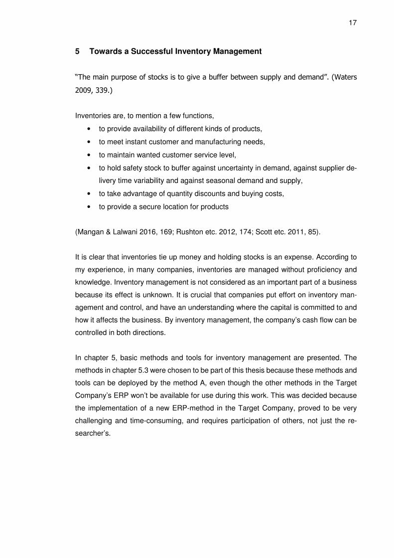
5.1 Inventory turnover
The inventory turnover measures, on average, how many times inventory is replaced
over a period of time. It is important measure since the ability to move inventory
quickly directly impacts the company’s liquidity
��������� ������� = � �� � ��� � �� � ��� �� � ������� ������ �� ���� , (1)
(Mangan & Lalwani 2016, 168; Muller 2003, 30; Sakki 2014, 55; Salmivuori 2010, 83).
Calculation can also be done for cost of goods sold from inventory only, it is a more
accurate measure of how many times actual physical inventory turned within the site
����� ℎ�"#��� #�������� ������� = � �� � � �� � �� �� $ ������ �� ���������� ������ �� , (2)
(Muller 2003, 31).
When 365 is divided by the inventory turnover, an average time to sell the inventory is
obtained. The obtained number also measures days the inventory remains still
��������� ������� #� %��" = &'(������ �� �)� ��� ���� , (3)
(Sakki 2014, 56).
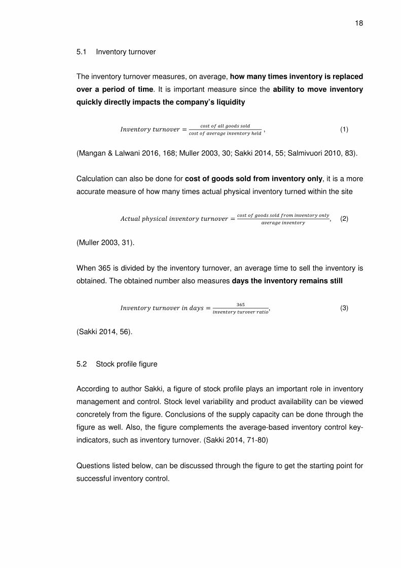
5.2 Stock profile figure
According to author Sakki, a figure of stock profile plays an important role in inventory
management and control. Stock level variability and product availability can be viewed
concretely from the figure. Conclusions of the supply capacity can be done through the
figure as well. Also, the figure complements the average-based inventory control key-
indicators, such as inventory turnover. (Sakki 2014, 71-80)
Questions listed below, can be discussed through the figure to get the starting point for
successful inventory control.
19
1. Stock levels in right relation to the demand?
2. Right amount purchased?
3. Timely purchased?
4. Stock necessity?
(Sakki 2014, 80; Waters 2009, 338; Salmivuori 2010, 51)
5.3 Inventory control methods
One important function of inventory control is to determine the right time and the right
amount to order (Hokkanen & Karhunen 2014, 207).
5.3.1 Safety stock
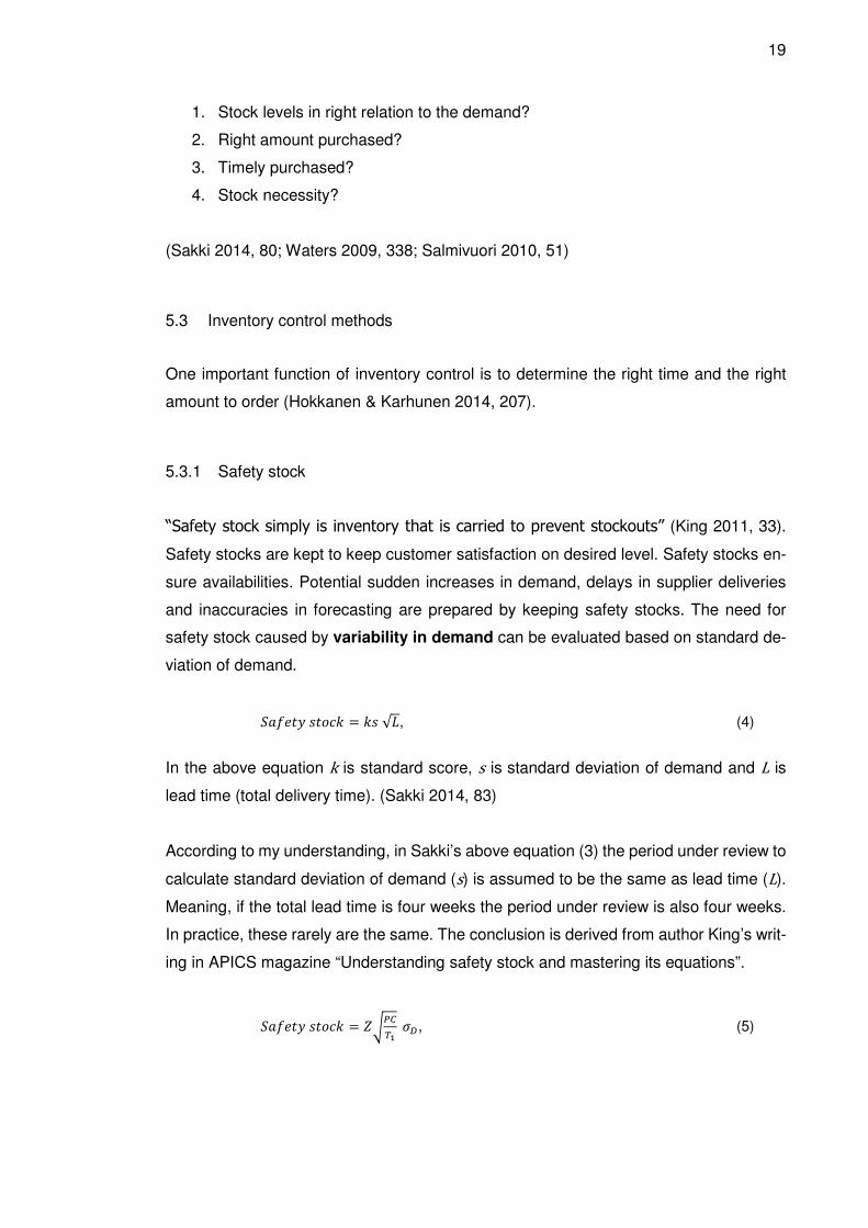
“Safety stock simply is inventory that is carried to prevent stockouts” (King 2011, 33).
Safety stocks are kept to keep customer satisfaction on desired level. Safety stocks en-
sure availabilities. Potential sudden increases in demand, delays in supplier deliveries
and inaccuracies in forecasting are prepared by keeping safety stocks. The need for
safety stock caused by variability in demand can be evaluated based on standard de-
viation of demand.
*�+��� "���, = ," √., (4)
In the above equation k is standard score, s is standard deviation of demand and L is
lead time (total delivery time). (Sakki 2014, 83)
According to my understanding, in Sakki’s above equation (3) the period under review to
calculate standard deviation of demand (s) is assumed to be the same as lead time (L).
Meaning, if the total lead time is four weeks the period under review is also four weeks.
In practice, these rarely are the same. The conclusion is derived from author King’s writ-
ing in APICS magazine “Understanding safety stock and mastering its equations”.
*�+��� "���, = 234567 89, (5)
20
In the above equation Z is standard score, PC is performance cycle (total lead time), =>
is time increment used for calculating standard deviation of demand and 89 is standard
deviation of demand. (King 2011, 34) The King’s above equation (4) is closer to a real
life, with the review period and performance cycle rarely equal.
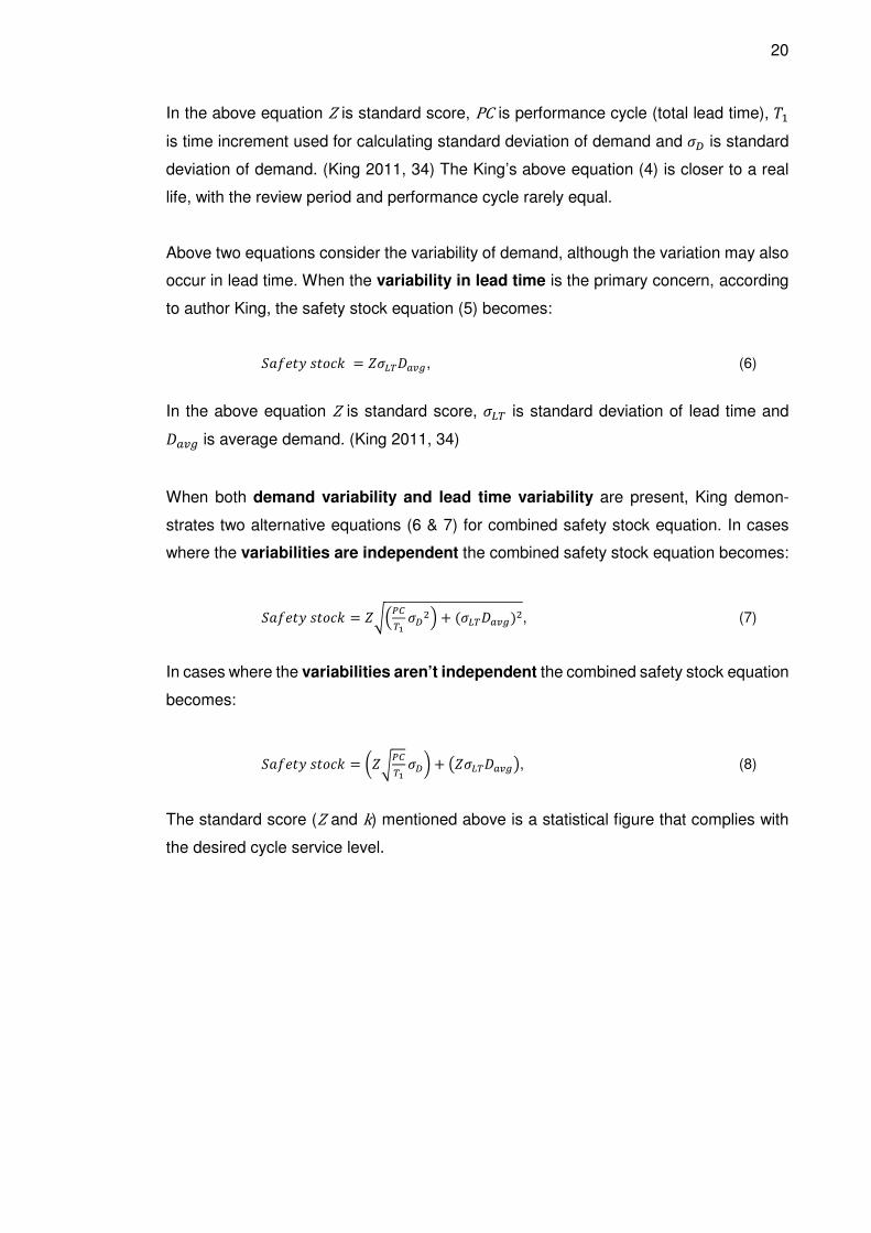
Above two equations consider the variability of demand, although the variation may also
occur in lead time. When the variability in lead time is the primary concern, according
to author King, the safety stock equation (5) becomes:
*�+��� "���, = 28?6@���, (6)
In the above equation Z is standard score, 8?6 is standard deviation of lead time and
@��� is average demand. (King 2011, 34)
When both demand variability and lead time variability are present, King demon-
strates two alternative equations (6 & 7) for combined safety stock equation. In cases
where the variabilities are independent the combined safety stock equation becomes:
*�+��� "���, = 23A4567 89BC + (8?6@���)B, (7)
In cases where the variabilities aren’t independent the combined safety stock equation
becomes:
*�+��� "���, = G234567 89H + I28?6@���J, (8)
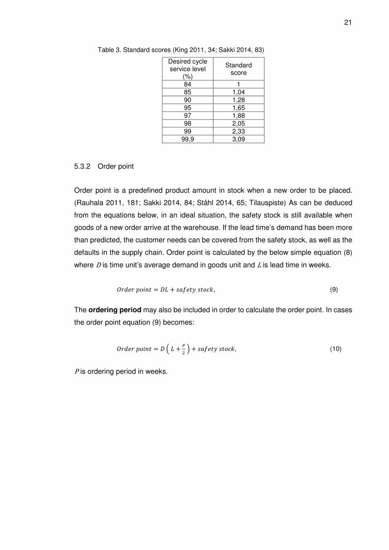
The standard score (Z and k) mentioned above is a statistical figure that complies with
the desired cycle service level.
21
Table 3. Standard scores (King 2011, 34; Sakki 2014, 83)
Desired cycle service level
(%)
Standard score
84 1 85 1,04 90 1,28 95 1,65 97 1,88 98 2,05 99 2,33
99,9 3,09
5.3.2 Order point
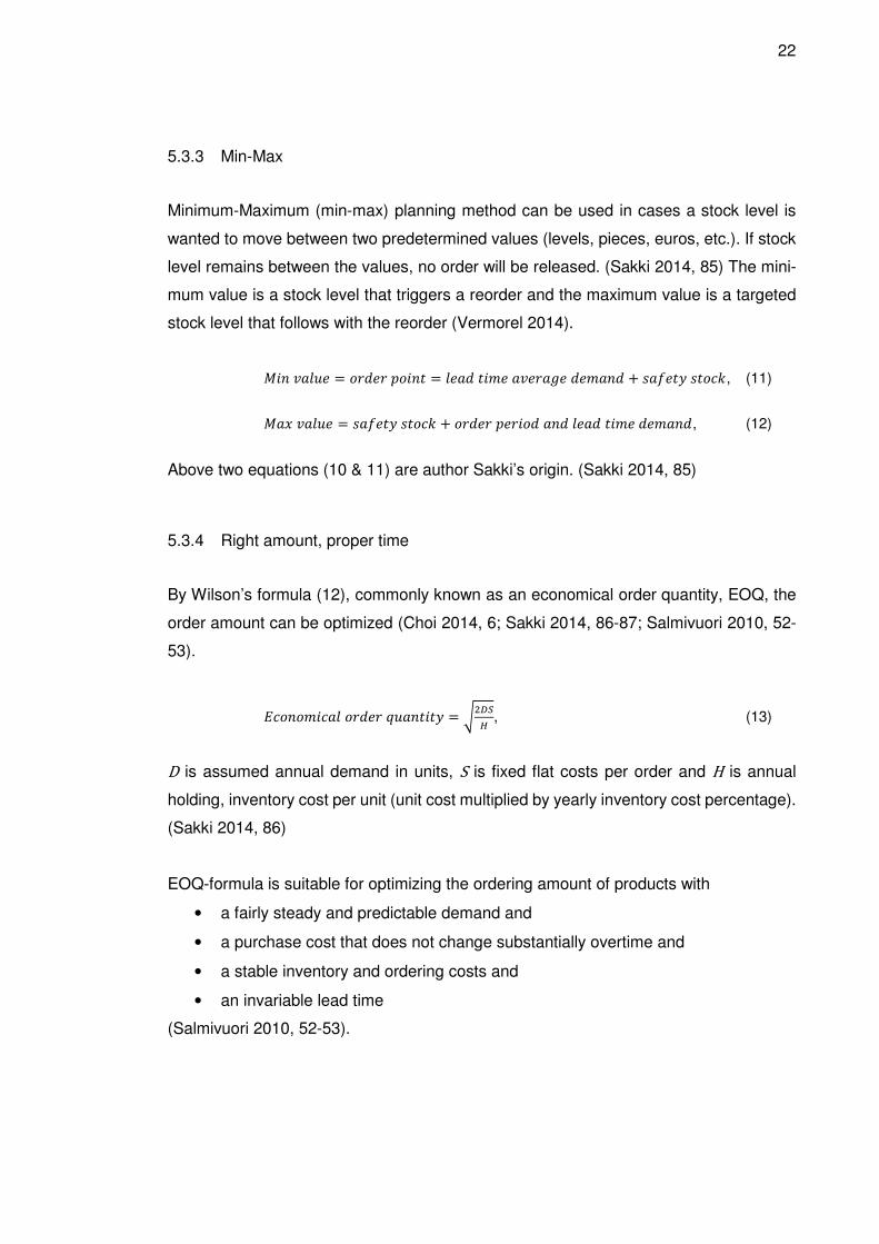
Order point is a predefined product amount in stock when a new order to be placed.
(Rauhala 2011, 181; Sakki 2014, 84; Ståhl 2014, 65; Tilauspiste) As can be deduced
from the equations below, in an ideal situation, the safety stock is still available when
goods of a new order arrive at the warehouse. If the lead time’s demand has been more
than predicted, the customer needs can be covered from the safety stock, as well as the
defaults in the supply chain. Order point is calculated by the below simple equation (8)
where D is time unit’s average demand in goods unit and L is lead time in weeks.
L�%�� �#�� = @. + "�+��� "���,, (9)
The ordering period may also be included in order to calculate the order point. In cases
the order point equation (9) becomes:
L�%�� �#�� = @ A . + 4B C + "�+��� "���,, (10)
P is ordering period in weeks.
22
5.3.3 Min-Max
Minimum-Maximum (min-max) planning method can be used in cases a stock level is
wanted to move between two predetermined values (levels, pieces, euros, etc.). If stock
level remains between the values, no order will be released. (Sakki 2014, 85) The mini-
mum value is a stock level that triggers a reorder and the maximum value is a targeted
stock level that follows with the reorder (Vermorel 2014).
M#� ���� = ��%�� �#�� = ���% �#N� �����O� %�N��% + "�+��� "���,, (11)
M�P ���� = "�+��� "���, + ��%�� ��#�% ��% ���% �#N� %�N��%, (12)
Above two equations (10 & 11) are author Sakki’s origin. (Sakki 2014, 85)
5.3.4 Right amount, proper time
By Wilson’s formula (12), commonly known as an economical order quantity, EOQ, the
order amount can be optimized (Choi 2014, 6; Sakki 2014, 86-87; Salmivuori 2010, 52-
53).
Q����N#��� ��%�� R���#�� = 3B9ST , (13)
D is assumed annual demand in units, S is fixed flat costs per order and H is annual
holding, inventory cost per unit (unit cost multiplied by yearly inventory cost percentage).
(Sakki 2014, 86)
EOQ-formula is suitable for optimizing the ordering amount of products with
• a fairly steady and predictable demand and
• a purchase cost that does not change substantially overtime and
• a stable inventory and ordering costs and
• an invariable lead time
(Salmivuori 2010, 52-53).
23
In cases, a supplier supplies more than one product to a company, adding products into
the same purchase order is sensible and cost-effective. By Wilson’s formula, the proper
ordering period can be calculated. According to author Sakki, the biggest expense is
associated with shipping of goods, so its worth of finding out, in how many shipments
the annual need should be divided to.
L�%�� ��#�% = 3B 6WXW 9, (14)
TK is a cost for one shipment (cost of freight + cost of purchasing + cost of handling
goods receipt), VK is an inventory cost percentage and D is an aggregate value of annual
need of the supplier’s all products. (Sakki 2014, 87)
5.3.5 Scrap the dead stock
Very often at my work, I’m in a situation, where I’m arguing against the opinion that any
of existing stock should not be disposed, even if the products in stock hasn’t been used
in years. Most commonly I’ve been told that we might use the products someday and
there’s a plenty of room in Inventory to keep them and also the products are already
paid, so why to dispose. My opinion is that all the products that accumulate costs only
and have no intended use or sale, should be disposed. The question is where to draw
the line? When a product is disposable?
24
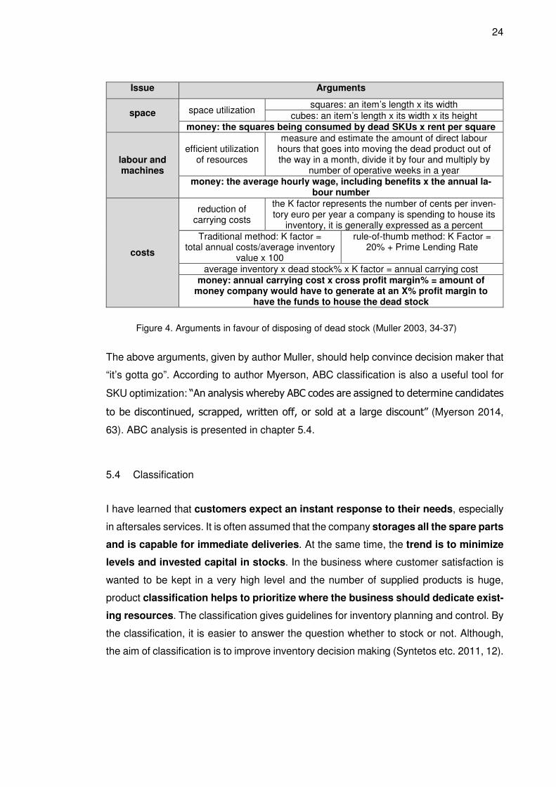
Issue Arguments
space space utilization squares: an item’s length x its width
cubes: an item’s length x its width x its height money: the squares being consumed by dead SKUs x rent per square
labour and machines
efficient utilization of resources
measure and estimate the amount of direct labour hours that goes into moving the dead product out of the way in a month, divide it by four and multiply by
number of operative weeks in a year money: the average hourly wage, including benefits x the annual la-
bour number
costs
reduction of carrying costs
the K factor represents the number of cents per inven-tory euro per year a company is spending to house its
inventory, it is generally expressed as a percent Traditional method: K factor =
total annual costs/average inventory value x 100
rule-of-thumb method: K Factor = 20% + Prime Lending Rate
average inventory x dead stock% x K factor = annual carrying cost money: annual carrying cost x cross profit margin% = amount of
money company would have to generate at an X% profit margin to have the funds to house the dead stock
Figure 4. Arguments in favour of disposing of dead stock (Muller 2003, 34-37)
The above arguments, given by author Muller, should help convince decision maker that
“it’s gotta go”. According to author Myerson, ABC classification is also a useful tool for
SKU optimization: “An analysis whereby ABC codes are assigned to determine candidates
to be discontinued, scrapped, written off, or sold at a large discount” (Myerson 2014,
63). ABC analysis is presented in chapter 5.4.
5.4 Classification
I have learned that customers expect an instant response to their needs, especially
in aftersales services. It is often assumed that the company storages all the spare parts
and is capable for immediate deliveries. At the same time, the trend is to minimize
levels and invested capital in stocks. In the business where customer satisfaction is
wanted to be kept in a very high level and the number of supplied products is huge,
product classification helps to prioritize where the business should dedicate exist-
ing resources. The classification gives guidelines for inventory planning and control. By
the classification, it is easier to answer the question whether to stock or not. Although,
the aim of classification is to improve inventory decision making (Syntetos etc. 2011, 12).
25
ABC analysis is a method used in many inventory systems to classify products. It is
based on Pareto principle, 20/80 rule. According to the rule, only a relatively few
products typically generate a large percentage of sales or profits. In the traditional
ABC classification, the products are classified in three classes A, B and C based on the
annual sales. A; 20% of items generate 80% of annual sales, B; next 50% generate 15%
of sales and C; last 30% generate only 5% of sales. (Myerson 2015, 61-63; Sakki 2014,
61-64; Salmivuori 2010, 37-38; Ståhl 2014, 63; Syntetos etc. 2011, 13) There are also
classifications in use with more than A, B and C classes (Synteos etc. 2011, 13).
The class A is considered as the most critical, to which products, existing resources
should be dedicated the most. Still, this doesn’t mean that the other classes are mean-
ingless. There are products, in the other classes, which are very important to the busi-
ness and/or the customers. The ABC classification emphases that handling the inventory
control, the product pricing and the customer service should be done differently on each
class (Myerson 2015, 62; Sakki 2014, 61).
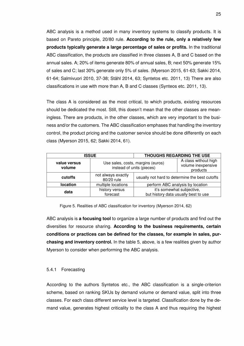
ISSUE THOUGHS REGARDING THE USE
value versus volume
Use sales, costs, margins (euros) instead of units (pieces)
A class without high volume inexpensive
products
cutoffs not always exactly
80/20 rule usually not hard to determine the best cutoffs
location multiple locations perform ABC analysis by location
data history versus
forecast it’s somewhat subjective,
but history data usually best to use
Figure 5. Realities of ABC classification for inventory (Myerson 2014, 62)
ABC analysis is a focusing tool to organize a large number of products and find out the
diversities for resource sharing. According to the business requirements, certain
conditions or practices can be defined for the classes, for example in sales, pur-
chasing and inventory control. In the table 5, above, is a few realities given by author
Myerson to consider when performing the ABC analysis.
5.4.1 Forecasting
According to the authors Syntetos etc., the ABC classification is a single-criterion
scheme, based on ranking SKUs by demand volume or demand value, split into three
classes. For each class different service level is targeted. Classification done by the de-
mand value, generates highest criticality to the class A and thus requiring the highest
26
service level to avoid backlogs. According to another argument, the class C should get
the highest service level to avoid stock outs on relatively inexpensive SKUs in inventory.
In summary Syntetos etc. notes that neither demand-value nor demand-volume cri-
terion has been developed from inventory perspective. (Syntetos etc. 2011, 13-15)
The ABC classification does not take forecasting into account. Faster-moving SKUs are
commonly forecast using time-series methods, but for items that are with lumpy demand,
time-series may not work. Problem is that the classification scheme based on demand
value or demand volume does not consider demand rate. Authors notes that a better
approach to classify items in a manner that facilitates the choice of appropriate forecast-
ing method. The authors identified two key classification criteria:
1. the degree of intermittence in demand
2. how erratic demand is when it occurs
(Syntetos etc. 2011, 13-15).
27
6 Optimizing & Implementing
6.1 Product group and goals for optimization
The purpose of inventory management is to know in a timely manner how many pieces
each product is at each inventory location. For a successful inventory management fol-
lowing things are to be known: location of the goods, amount of the goods, arrivals and
dispatches of the goods, availabilities and needs of the goods, amount of incoming goods
and whether stock amounts and set stock levels are in right balance. (Ståhl 2014, 55-56)
Since it was not possible to optimize the entire Service stock within the thesis, the scope
was limited to one specific product group. The product group was created to contain
same kind of products which were to be stored and were to be purchased from the same
supplier. Annual needs between different products in the product group were variable
and therefore, different ways to control stock were needed for optimization. The product
group contains 34 products. More information about the product group is in appendix 1.
The appendix 1 is not published because it contains company confidential information.
The objectives for inventory management and its control were derived from the key per-
formances of the Target Company’s Spare part business. There are different KPIs set to
measure the effectiveness and to guide the actions in spare part function. The status of
the KPIs are monitored in weekly basis and reported monthly. Two of the KPIs are related
to product availability and therefore directly effect on inventory management and stock
control. More information about the KPIs are in appendix 1. The appendix 1 is not pub-
lished because it contains company confidential information.
When planning inventory availability, it must be taken into account that usually cus-
tomer’s spare part orders are combined orders of different products. In this case, even if
the SKUs are all available from stock, it doesn’t mean that the 100% of customer orders
are delivered on confirmed date or on-time. The confirmed delivery date depends on the
other products that are combined in the same customer order. Basically, the KPIs are
not directly usable in inventory availability planning but they can be taken for guidance.
The Spare part business’ main purpose is to serve the customers in the best possible
way. From inventory management perspective, the purpose is filled by ensuring stock
28
availabilities of demanded products. Of course, all spare parts are not to be stored but
the ones which are important to customers. One other thing to keep in mind when plan-
ning the availabilities is that stocks are to be kept also to serve the Target Company’s
business in the best possible way. Storing goods means fast invoicing from receipt of
customer order, but on the other hand, storing is always a cost and binds money. Finding
the right balance is the best solution for keeping the businesses running (customers’ and
the Target Company’s). The more efficient the inventory management and the purchas-
ing activities are, the better the customer satisfaction will be, and the continuity of the
business is ensured. All this has a bearing on customer satisfaction, and good customer
satisfaction will promote more trade in the future.
6.2 Inventory availability planning
A goal of acquisition is to buy the right amount of the right quality at the right time at the
right price from the right provider to the right place (Ståhl 2014, 90). This is a classic,
passive, reactive understanding of procurement and purchasing. One of my personal
goal as a purchaser is to enable proactive purchasing. To be able to proactively take
action and get benefits of upcoming changes in business environment and supplier field,
instead of adapting to the changes that have already happened and just settling for them.
(Iloranta etc. 2015, 95)
To reach the goal above, the amount of purchaser’s operational work is to be reduced.
It can be done by the inventory-managed purchasing so that stock availability meets the
future demand;
• the SKUs are identified,
• inventory availability planning parameters that guide the SKUs’ acquisition are
optimized, and
• order proposals and order placing are handled automatically by ERP system.
It is clear that all the operational purchasing work can’t be, neither wanted to be, led by
the inventory management, but should be used when appropriate and reasonable.
After each products visualization (chapter 6.3; appendix 2), I divided the products into
groups based on the results of optimization. The product groups are presented in chapter
6.4. The products that had no demand in 2016 and 2017, and despite the fact that these
29
products should be stored, I decided to give my recommendation to the management
that these products will no longer be stored for just in case. In case of a demand, the
product will be purchased with the requested quantity and by express delivery. By ex-
press delivery, we are able to reduce the total lead time in weeks, if the order amount is
not more than ten pieces. Express delivery is a lot more expensive, but this could be
taken into account on sales pricing. According to this, following products will be pur-
chased after the demand has occurred and the requested amount only, no storing al-
lowed. The products are product1, product14, product25, product27, product33, prod-
uct3 and Product16. This rule was implemented to the Target Company’s ERP on March
2018. Now the system gives a purchase requisition of requested quantity when the sales
releases the customer order. Now purchasing doesn’t have to use time to find out
whether to store the product or not and how many pieces to purchase. The EOQ formula
(13) presented in chapter 5.3.4, is not used as a planning method in this paper because
none of the products contained the conditions required for the use.
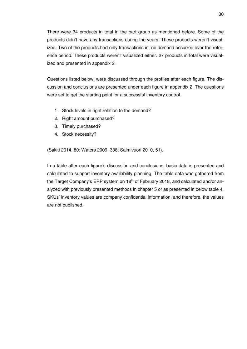
6.3 Visualizing
To get a better understanding of the products’ nature, I decided to make figures of stock
profiles of each product. Stock profiles present product’s stock level movements and
transactions in and out in 2016 and 2017 (figure 6). Data, to make profiles, were gathered
from the Target Company’s ERP system on 18th of February 2018. The illustration of the
stock profile figures were inspired by author Sakki (Sakki 2014, 78-79). The stock profiles
are presented in appendix 2.
Figure 6. Stock profiles example, 2016 and 2017
30
There were 34 products in total in the part group as mentioned before. Some of the
products didn’t have any transactions during the years. These products weren’t visual-
ized. Two of the products had only transactions in, no demand occurred over the refer-
ence period. These products weren’t visualized either. 27 products in total were visual-
ized and presented in appendix 2.
Questions listed below, were discussed through the profiles after each figure. The dis-
cussion and conclusions are presented under each figure in appendix 2. The questions
were set to get the starting point for a successful inventory control.
1. Stock levels in right relation to the demand?
2. Right amount purchased?
3. Timely purchased?
4. Stock necessity?
(Sakki 2014, 80; Waters 2009, 338; Salmivuori 2010, 51).
In a table after each figure’s discussion and conclusions, basic data is presented and
calculated to support inventory availability planning. The table data was gathered from
the Target Company’s ERP system on 18th of February 2018, and calculated and/or an-
alyzed with previously presented methods in chapter 5 or as presented in below table 4.
SKUs’ inventory values are company confidential information, and therefore, the values
are not published.
31
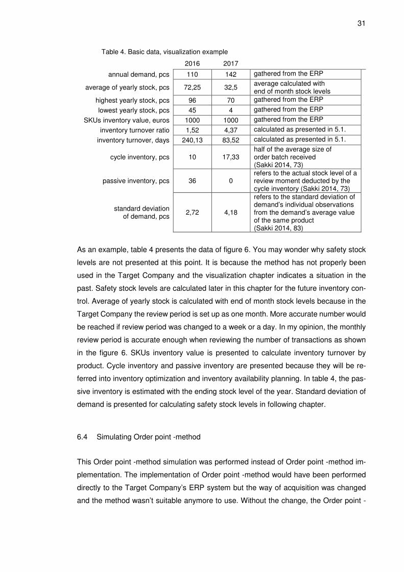
Table 4. Basic data, visualization example
2016 2017
annual demand, pcs 110 142 gathered from the ERP
average of yearly stock, pcs 72,25 32,5 average calculated with end of month stock levels
highest yearly stock, pcs 96 70 gathered from the ERP
lowest yearly stock, pcs 45 4 gathered from the ERP
SKUs inventory value, euros 1000 1000 gathered from the ERP
inventory turnover ratio 1,52 4,37 calculated as presented in 5.1.
inventory turnover, days 240,13 83,52 calculated as presented in 5.1.
cycle inventory, pcs 10 17,33 half of the average size of order batch received (Sakki 2014, 73)
passive inventory, pcs 36 0 refers to the actual stock level of a review moment deducted by the cycle inventory (Sakki 2014, 73)
standard deviation of demand, pcs
2,72 4,18
refers to the standard deviation of demand’s individual observations from the demand’s average value of the same product (Sakki 2014, 83)
As an example, table 4 presents the data of figure 6. You may wonder why safety stock
levels are not presented at this point. It is because the method has not properly been
used in the Target Company and the visualization chapter indicates a situation in the
past. Safety stock levels are calculated later in this chapter for the future inventory con-
trol. Average of yearly stock is calculated with end of month stock levels because in the
Target Company the review period is set up as one month. More accurate number would
be reached if review period was changed to a week or a day. In my opinion, the monthly
review period is accurate enough when reviewing the number of transactions as shown
in the figure 6. SKUs inventory value is presented to calculate inventory turnover by
product. Cycle inventory and passive inventory are presented because they will be re-
ferred into inventory optimization and inventory availability planning. In table 4, the pas-
sive inventory is estimated with the ending stock level of the year. Standard deviation of
demand is presented for calculating safety stock levels in following chapter.
6.4 Simulating Order point -method
This Order point -method simulation was performed instead of Order point -method im-
plementation. The implementation of Order point -method would have been performed
directly to the Target Company’s ERP system but the way of acquisition was changed
and the method wasn’t suitable anymore to use. Without the change, the Order point -
32
method would have been chosen to perform inventory control and inventory-managed
purchasing.
The simulation should have been done anyway since the results can be analysed not
until the implemented stock control method and its parameters have been in use for
about a year. This is because the nature of the demands is intermittent and lumpy. This
simulation was done to investigate how the optimization would have affected the inven-
tory levels in 2017 and to get indicative results and conclusions of the performed optimi-
zation. The Order point -method will be taken in use in the Target Company but not for
the product group.
The output data for this simulation was gathered from the Target Company’s ERP sys-
tem. The data of 2016 was used to optimize the inventory of 2017. The calculations in
the optimization were performed using only data that was available in the end of 2016 to
achieve realistic results and conclusions from the simulation.
Safety stock levels were calculated based on the equation in which the demand is con-
sidered as variable and variability of lead time is not taken into account because in this
case it is invariable. Therefore, the other introduced safety stock equations (4, 6, 7 and
8) were not chosen. The chosen safety stock equation (5) is introduced in chapter 5.3.1
as well the others. Order points were calculated based on the equation (9) introduced in
chapter 5.3.2. Order quantity was defined in this simulation to match the lead time’s av-
erage demand.
Based on the results of the optimization, the products were divided in four groups named
Orange (6.4.1), Yellow (6.4.2), Blue (6.4.2) and Green (6.4.3). The reasons for the divi-
sion can be found in the chapters. In each chapter, simulations are presented with tables.
The tables contain of three different sections. The first section, grey-section, contains the
results of the optimization i.e. the stock control parameters, and a total demand in 2016
-figure that was used for calculating the parameters. Presented parameters are safety
stock, order point and order quantity. The second section, white-section, contains infor-
mation related to purchasing and the actual figures in 2017. Purchasing related infor-
mation is products minimum order quantity and a multiple lot size. The actual figures
contain the figures of total demand in 2017, average yearly stock level in 2017 and in-
ventory turnover rate in 2017. The last section, which is colored after the group name,
contain results of the simulation. Presented results are yearly stock optimized, inventory
33
turnover optimized, inventory turnover change and average yearly stock value change.
Group chapters are followed by Results -chapter where the results of the simulation are
introduced and summarized (Chapter 6.5.1).
6.4.1 Orange
This chapter deals with products of which stock control was performed using the Order
point –method. Stock control parameters were reviewed quarterly.
Group Orange consists of products with cyclical demand, calculated safety stock
level as well as total demand in 2016 was more than zero and calculated order quan-
tity was more than minimum order quantity.
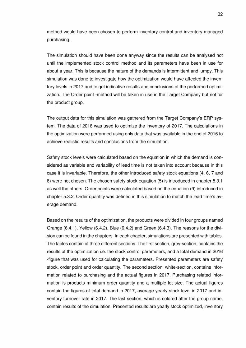
In table 5 products with cyclic demand are listed with values.
Table 5. Cyclic demand
Products in table 5, total ten pieces, were all simulated as the Order point -method would
have controlled the purchasing in 2017. Meaning the stock control parameters; safety
stock, order point and order quantity, remained as they were calculated (optimized) in
the first place. Only one exception done with the product12. Order point and order quan-
tity parameters were reset in the beginning of Q2 because in the quarterly monitoring
would have been observed that the demand of the first quarter was more than the total
demand in 2016. Updated parameters were calculated based on the first quarter in 2017.
Poduct
Total
Demand
2016
Safety
Stock
Order
Point
Order
Quantity
Min.
Order
Quantity
& Multiple
Lot Size
Total
Demand
2017
Average
Yearly
Stock
2017
Inventory
Turnover
2017
Average
of Yearly
Stock
Optimized
Inventory
Turnover
Optimized
product2 110 17 32 16 4 142 32.5 4.37 7.67 18.51
product7 10 2 4 2 2 10 10.67 0.94 7.17 1.39
product11 48 10 17 6 2 42 16.83 2.50 11.33 3.71
product12 13 4 Q2: 6 16 2 12 2 69 21.33 3.23 20.83 3.31
product13 68 8 17 10 2 73 21.67 3.37 11.50 6.35
product15 67 11 20 10 2 38 28.17 1.35 22.83 1.66
product21 22 3 6 4 2 20 5.42 3.69 4.25 4.71
product23 9 2 3 2 2 8 1.67 4.79 3 2.67
product26 5 2 2 2 2 3 0.67 4.48 2.67 1.12
product34 94 13 25 14 4 78 9.33 8.36 15.42 5.06
34
6.4.2 Yellow and Blue
This chapter deals with products of which stock control was performed using the Order
point –method. Stock control parameters were reviewed twice a year.
Group Yellow and Blue consist of products that calculated stock control parameters
were zero or calculated order quantity was less that minimum order quantity and
total demand in 2016 were more than zero.
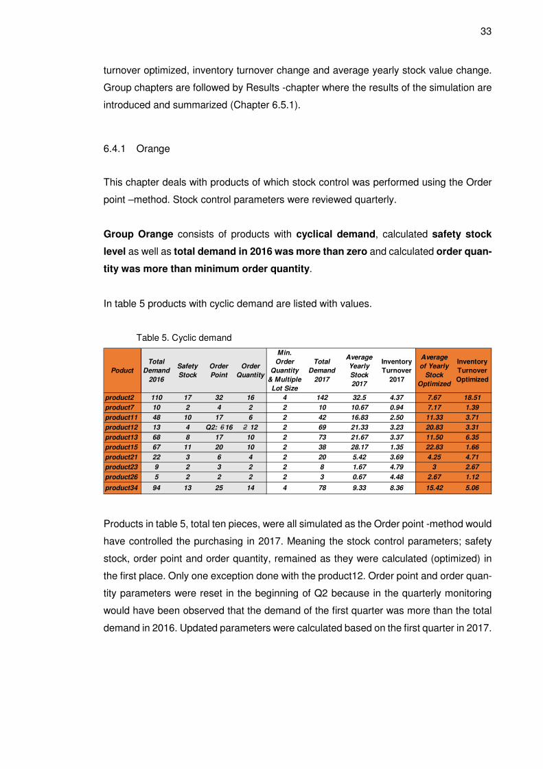
In table 6 products with predictable demand are listed with values.
Table 6. Predictable demand
Table 6 consists of two products, group Yellow. Stock control parameters were reset
before the simulation because calculated parameters were: safety stock = 0, order point
= 1 and order quantity = 1, and since the minimum order quantity for both product was
two pieces, I changed the order quantity to two pieces. Calculated order point was one
piece, but since the total demand in 2016 per product, was four pieces and in 2016 cus-
tomers ordered two pieces at a time, I decided to change the order point to be zero.
Parameters used in the simulation were safety stock = 0, order point = 0 and order quan-
tity = 2. It means that the products would be purchased when the stock levels reach the
zero. I assumed that the products would be purchased in batches of two pieces also in
2017 and that the demand can be called as “predictable demand”. No changes done
over the monitoring periods.
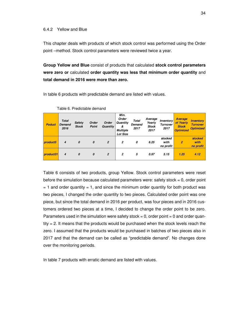
In table 7 products with erratic demand are listed with values.
Poduct
Total
Demand
2016
Safety
Stock
Order
Point
Order
Quantity
Min.
Order
Quantity
&
Multiple
Lot Size
Total
Demand
2017
Average
Yearly
Stock
2017
Inventory
Turnover
2017
Average
of Yearly
Stock
Optimized
Inventory
Turnover
Optimized
product5 4 0 0 2 2 0 6.25
stocked
with
no profit
2
stocked
with
no profit
product31 4 0 0 2 2 5 0.97 5.15 1.25 4.12
35
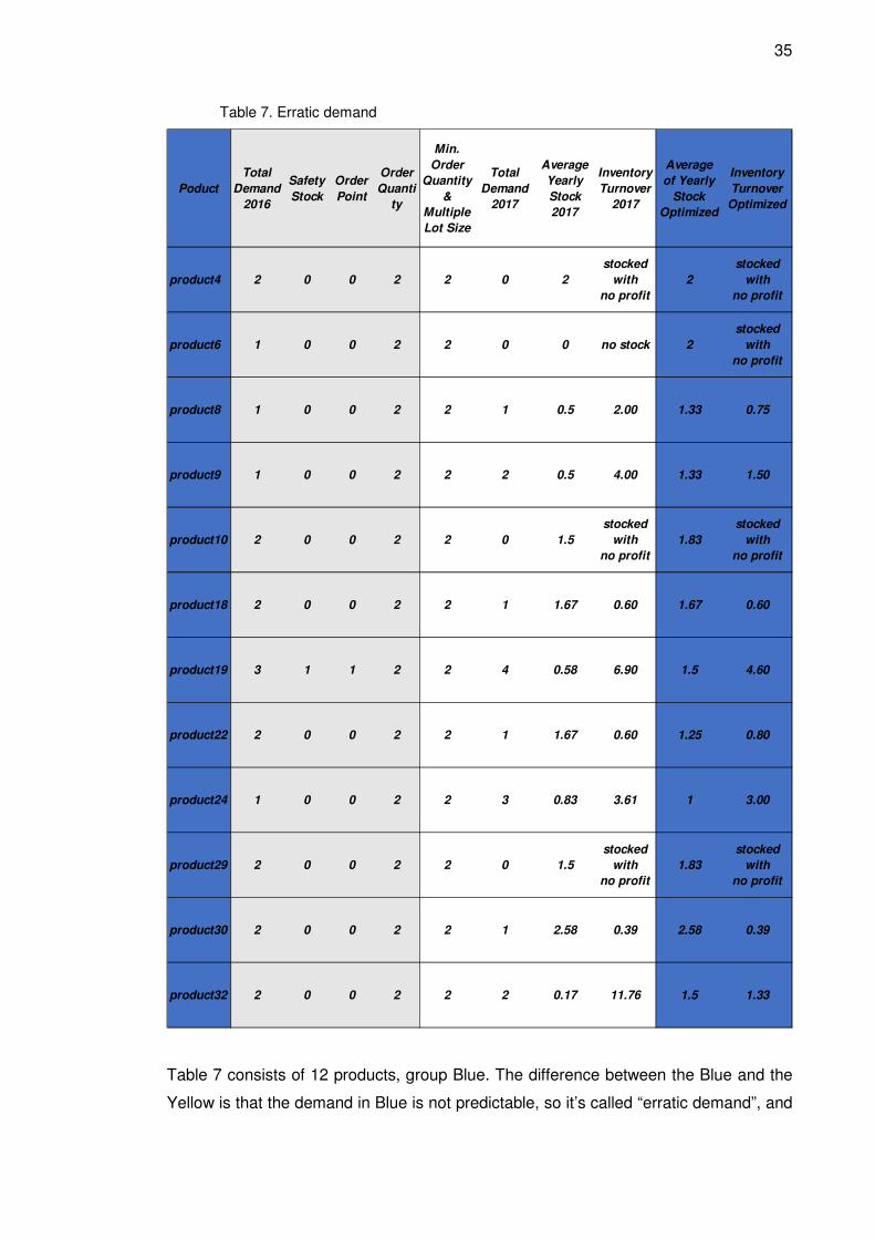
Table 7. Erratic demand
Table 7 consists of 12 products, group Blue. The difference between the Blue and the
Yellow is that the demand in Blue is not predictable, so it’s called “erratic demand”, and
Poduct
Total
Demand
2016
Safety
Stock
Order
Point
Order
Quanti
ty
Min.
Order
Quantity
&
Multiple
Lot Size
Total
Demand
2017
Average
Yearly
Stock
2017
Inventory
Turnover
2017
Average
of Yearly
Stock
Optimized
Inventory
Turnover
Optimized
product4 2 0 0 2 2 0 2
stocked
with
no profit
2
stocked
with
no profit
product6 1 0 0 2 2 0 0 no stock 2
stocked
with
no profit
product8 1 0 0 2 2 1 0.5 2.00 1.33 0.75
product9 1 0 0 2 2 2 0.5 4.00 1.33 1.50
product10 2 0 0 2 2 0 1.5
stocked
with
no profit
1.83
stocked
with
no profit
product18 2 0 0 2 2 1 1.67 0.60 1.67 0.60
product19 3 1 1 2 2 4 0.58 6.90 1.5 4.60
product22 2 0 0 2 2 1 1.67 0.60 1.25 0.80
product24 1 0 0 2 2 3 0.83 3.61 1 3.00
product29 2 0 0 2 2 0 1.5
stocked
with
no profit
1.83
stocked
with
no profit
product30 2 0 0 2 2 1 2.58 0.39 2.58 0.39
product32 2 0 0 2 2 2 0.17 11.76 1.5 1.33
36
the results of made calculations achieving parameters, were less than one in all figures.
As mentioned, calculated order points were zero but since the total demand in 2016 by
product was more than zero, I decided to make an assumption that the products would
have demand also in 2017. I decided to set the safety stocks and order points to zero
and order quantities according to the minimum order quantity which is in these cases
two pieces. This means that when the stock level reach the zero the order will be created
for two pieces. In other words, there will be stock or at least new purchase order released
all the time. There is one exception in the Blue group, product19. Calculated parameters
were safety stock = 1,30, order point = 0,70 and order quantity = 0,40. I changed them
to be safety stock = 1, order point = 1 and order quantity = 2. No changes done for Blues
over the monitoring periods.
6.4.3 Green
This chapter deals with products of which stock control was performed using the Order
point –method. Stock control parameters were reviewed twice a year.
Group Green consist of products that total demand in 2016 was zero.
In table 8 products with zero demand are listed with values.
37
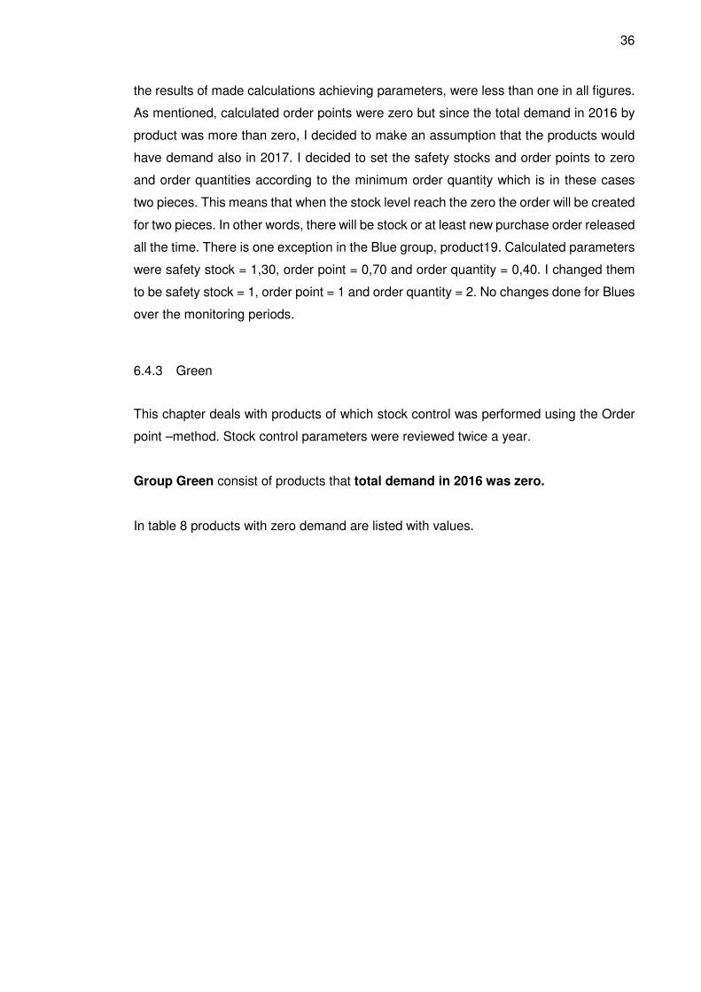
Table 8. No demand
Table 8 consists of 10 products, group Green. Optimization performed by the Order point
-method weren’t possible for the Greens since there was no demand at all in 2016. Even
though the products should be stored, I decided not to do that and release the purchases
only after the receipt of a customer order (CO). Then, the purchase order quantity de-
pends on the customer order amount and/or the minimum order quantity (CO/min.o.qty).
At the same time, I made a decision that possible customer needs are not to be met
immediately.
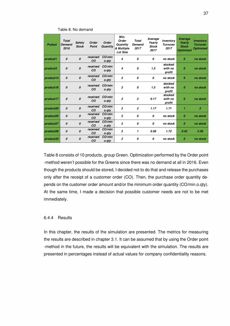
6.4.4 Results
In this chapter, the results of the simulation are presented. The metrics for measuring
the results are described in chapter 3.1. It can be assumed that by using the Order point
-method in the future, the results will be equivalent with the simulation. The results are
presented in percentages instead of actual values for company confidentiality reasons.
Poduct
Total
Demand
2016
Safety
Stock
Order
Point
Order
Quantity
Min.
Order
Quantity
& Multiple
Lot Size
Total
Demand
2017
Average
Yearly
Stock
2017
Inventory
Turnover
2017
Average
Yearly
Stock
Optimized
Inventory
Turnover
Optimized
product1 0 0received
CO
CO/min
o.qty4 0 0 no stock 0 no stock
product3 0 0received
CO
CO/min
o.qty4 0 1.5
stocked
with no
profit
0 no stock
product14 0 0received
CO
CO/min
o.qty2 0 0 no stock 0 no stock
product16 0 0received
CO
CO/min
o.qty2 0 1.5
stocked
with no
profit
0 no stock
product17 0 0received
CO
CO/min
o.qty2 2 0.17
stocked
with no
profit
0 no stock
product20 0 0received
CO
CO/min
o.qty2 2 1.17 1.71 1 2
product25 0 0received
CO
CO/min
o.qty2 0 0 no stock 0 no stock
product27 0 0received
CO
CO/min
o.qty2 0 0 no stock 0 no stock
product28 0 0received
CO
CO/min
o.qty2 1 0.58 1.72 0.42 2.38
product33 0 0received
CO
CO/min
o.qty2 0 0 no stock 0 no stock
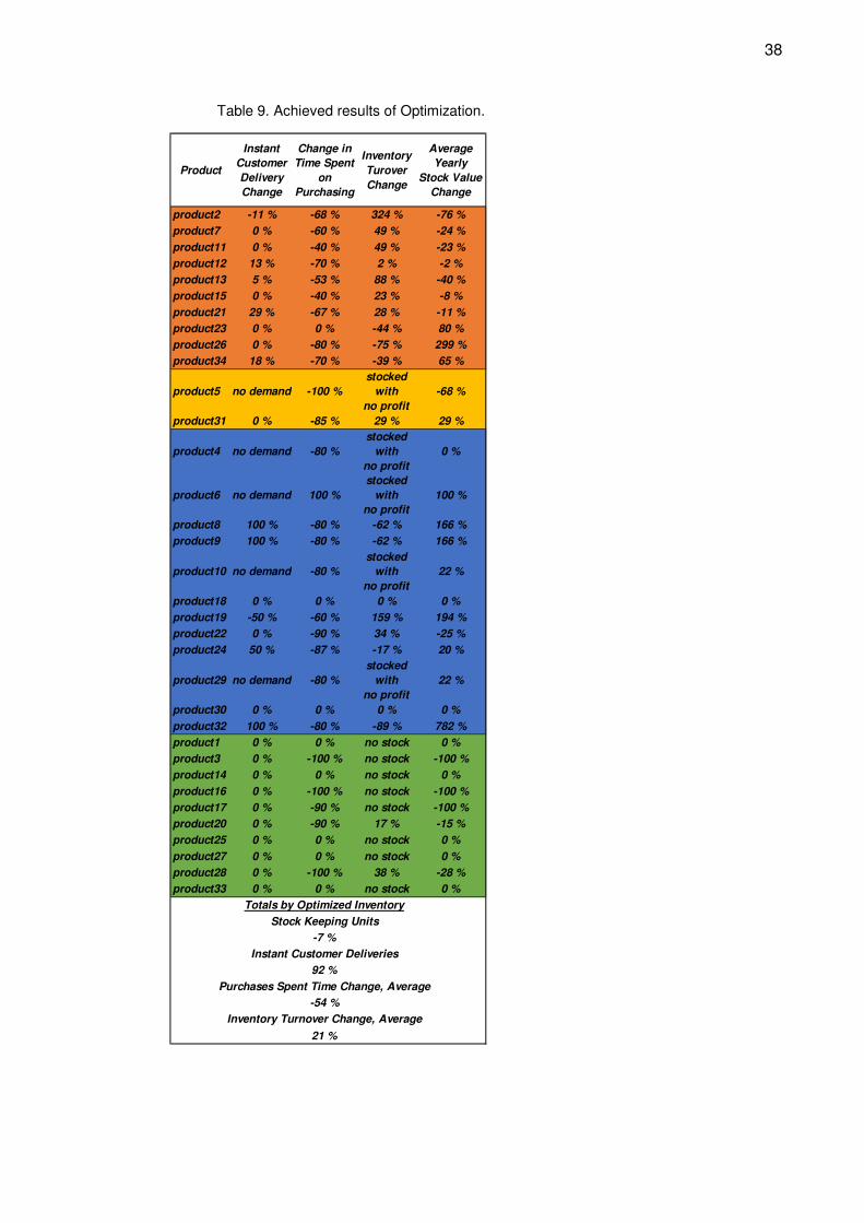
38
Table 9. Achieved results of Optimization.
Product
Instant
Customer
Delivery
Change
Change in
Time Spent
on
Purchasing
Inventory
Turover
Change
Average
Yearly
Stock Value
Change
product2 -11 % -68 % 324 % -76 %
product7 0 % -60 % 49 % -24 %
product11 0 % -40 % 49 % -23 %
product12 13 % -70 % 2 % -2 %
product13 5 % -53 % 88 % -40 %
product15 0 % -40 % 23 % -8 %
product21 29 % -67 % 28 % -11 %
product23 0 % 0 % -44 % 80 %
product26 0 % -80 % -75 % 299 %
product34 18 % -70 % -39 % 65 %
product5 no demand -100 %
stocked
with
no profit
-68 %
product31 0 % -85 % 29 % 29 %
product4 no demand -80 %
stocked
with
no profit
0 %
product6 no demand 100 %
stocked
with
no profit
100 %
product8 100 % -80 % -62 % 166 %
product9 100 % -80 % -62 % 166 %
product10 no demand -80 %
stocked
with
no profit
22 %
product18 0 % 0 % 0 % 0 %
product19 -50 % -60 % 159 % 194 %
product22 0 % -90 % 34 % -25 %
product24 50 % -87 % -17 % 20 %
product29 no demand -80 %
stocked
with
no profit
22 %
product30 0 % 0 % 0 % 0 %
product32 100 % -80 % -89 % 782 %
product1 0 % 0 % no stock 0 %
product3 0 % -100 % no stock -100 %
product14 0 % 0 % no stock 0 %
product16 0 % -100 % no stock -100 %
product17 0 % -90 % no stock -100 %
product20 0 % -90 % 17 % -15 %
product25 0 % 0 % no stock 0 %
product27 0 % 0 % no stock 0 %
product28 0 % -100 % 38 % -28 %
product33 0 % 0 % no stock 0 %
Totals by Optimized Inventory
Stock Keeping Units
-7 %
Instant Customer Deliveries
92 %
Purchases Spent Time Change, Average
-54 %
Inventory Turnover Change, Average
21 %
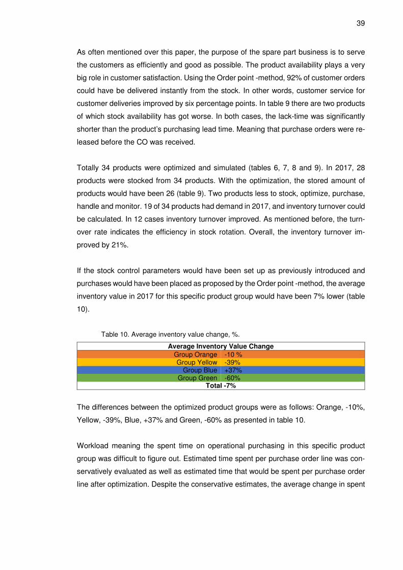
39
As often mentioned over this paper, the purpose of the spare part business is to serve
the customers as efficiently and good as possible. The product availability plays a very
big role in customer satisfaction. Using the Order point -method, 92% of customer orders
could have be delivered instantly from the stock. In other words, customer service for
customer deliveries improved by six percentage points. In table 9 there are two products
of which stock availability has got worse. In both cases, the lack-time was significantly
shorter than the product’s purchasing lead time. Meaning that purchase orders were re-
leased before the CO was received.
Totally 34 products were optimized and simulated (tables 6, 7, 8 and 9). In 2017, 28
products were stocked from 34 products. With the optimization, the stored amount of
products would have been 26 (table 9). Two products less to stock, optimize, purchase,
handle and monitor. 19 of 34 products had demand in 2017, and inventory turnover could
be calculated. In 12 cases inventory turnover improved. As mentioned before, the turn-
over rate indicates the efficiency in stock rotation. Overall, the inventory turnover im-
proved by 21%.
If the stock control parameters would have been set up as previously introduced and
purchases would have been placed as proposed by the Order point -method, the average
inventory value in 2017 for this specific product group would have been 7% lower (table
10).
Table 10. Average inventory value change, %.
Average Inventory Value Change
Group Orange -10 % Group Yellow -39%
Group Blue +37% Group Green -60%
Total -7%
The differences between the optimized product groups were as follows: Orange, -10%,
Yellow, -39%, Blue, +37% and Green, -60% as presented in table 10.
Workload meaning the spent time on operational purchasing in this specific product
group was difficult to figure out. Estimated time spent per purchase order line was con-
servatively evaluated as well as estimated time that would be spent per purchase order
line after optimization. Despite the conservative estimates, the average change in spent
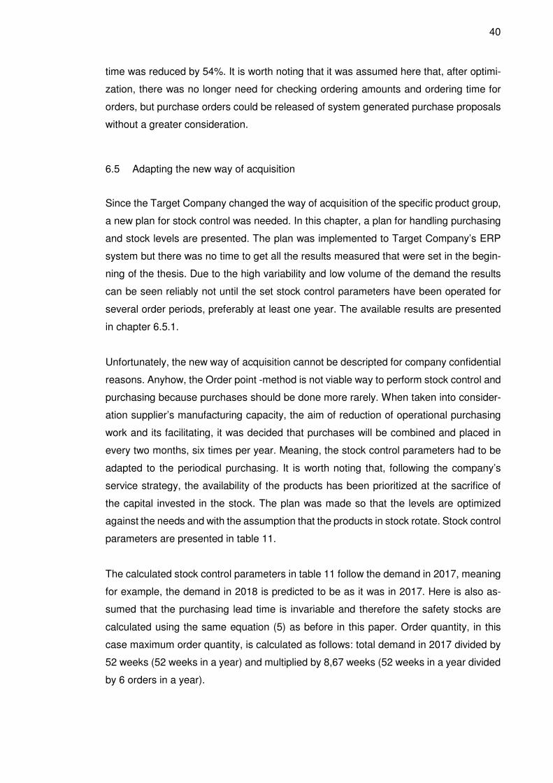
40
time was reduced by 54%. It is worth noting that it was assumed here that, after optimi-
zation, there was no longer need for checking ordering amounts and ordering time for
orders, but purchase orders could be released of system generated purchase proposals
without a greater consideration.
6.5 Adapting the new way of acquisition
Since the Target Company changed the way of acquisition of the specific product group,
a new plan for stock control was needed. In this chapter, a plan for handling purchasing
and stock levels are presented. The plan was implemented to Target Company’s ERP
system but there was no time to get all the results measured that were set in the begin-
ning of the thesis. Due to the high variability and low volume of the demand the results
can be seen reliably not until the set stock control parameters have been operated for
several order periods, preferably at least one year. The available results are presented
in chapter 6.5.1.
Unfortunately, the new way of acquisition cannot be descripted for company confidential
reasons. Anyhow, the Order point -method is not viable way to perform stock control and
purchasing because purchases should be done more rarely. When taken into consider-
ation supplier’s manufacturing capacity, the aim of reduction of operational purchasing
work and its facilitating, it was decided that purchases will be combined and placed in
every two months, six times per year. Meaning, the stock control parameters had to be
adapted to the periodical purchasing. It is worth noting that, following the company’s
service strategy, the availability of the products has been prioritized at the sacrifice of
the capital invested in the stock. The plan was made so that the levels are optimized
against the needs and with the assumption that the products in stock rotate. Stock control
parameters are presented in table 11.
The calculated stock control parameters in table 11 follow the demand in 2017, meaning
for example, the demand in 2018 is predicted to be as it was in 2017. Here is also as-
sumed that the purchasing lead time is invariable and therefore the safety stocks are
calculated using the same equation (5) as before in this paper. Order quantity, in this
case maximum order quantity, is calculated as follows: total demand in 2017 divided by
52 weeks (52 weeks in a year) and multiplied by 8,67 weeks (52 weeks in a year divided
by 6 orders in a year).
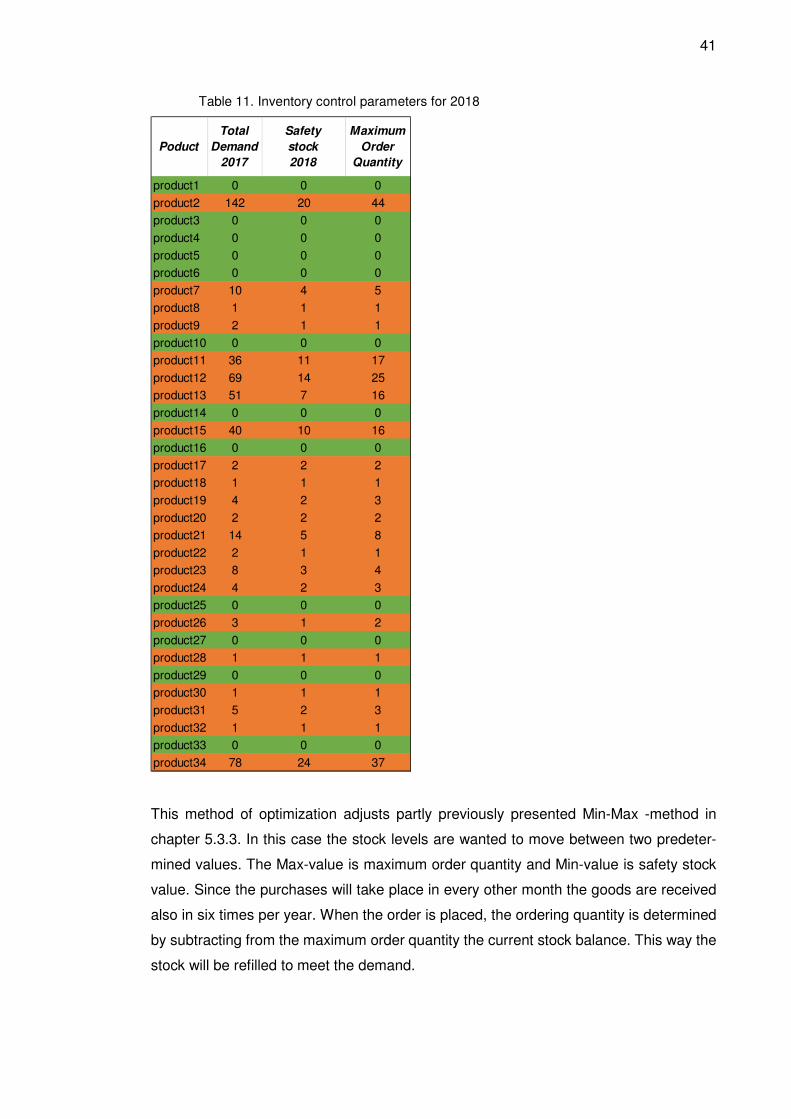
41
Table 11. Inventory control parameters for 2018
This method of optimization adjusts partly previously presented Min-Max -method in
chapter 5.3.3. In this case the stock levels are wanted to move between two predeter-
mined values. The Max-value is maximum order quantity and Min-value is safety stock
value. Since the purchases will take place in every other month the goods are received
also in six times per year. When the order is placed, the ordering quantity is determined
by subtracting from the maximum order quantity the current stock balance. This way the
stock will be refilled to meet the demand.
Total
Demand
2017
Safety
stock
2018
Maximum
Order
Quantity
product1 0 0 0
product2 142 20 44
product3 0 0 0
product4 0 0 0
product5 0 0 0
product6 0 0 0
product7 10 4 5
product8 1 1 1
product9 2 1 1
product10 0 0 0
product11 36 11 17
product12 69 14 25
product13 51 7 16
product14 0 0 0
product15 40 10 16
product16 0 0 0
product17 2 2 2
product18 1 1 1
product19 4 2 3
product20 2 2 2
product21 14 5 8
product22 2 1 1
product23 8 3 4
product24 4 2 3
product25 0 0 0
product26 3 1 2
product27 0 0 0
product28 1 1 1
product29 0 0 0
product30 1 1 1
product31 5 2 3
product32 1 1 1
product33 0 0 0
product34 78 24 37
Poduct
42
6.5.1 Results
The results of the implementation for the specific product group for year 2018 using the
Order period -method are presented in this chapter. The metrics for measuring the re-
sults are described in chapter 3.1.
Table 12. Placed orders in Q1, 2018
At this point the change in customer service cannot be measured. Still, it can be con-
cluded that since the safety stocks and order quantities are calculated in accordance
Beginning
stock in
January
2018
Beginning
stock in
March
2018
Ordered
in January
2018
Ordered
in March
2018
product1 0 0 0 0
product2 4 0 40 44
product3 2 2 0 0
product4 2 2 0 0
product5 8 8 0 0
product6 0 0 0 0
product7 7 5 0 0
product8 1 1 0 0
product9 2 2 0 0
product10 2 2 0 0
product11 7 7 10 10
product12 44 36 0 0
product13 13 7 3 9
product14 1 1 0 0
product15 12 8 4 8
product16 2 2 0 0
product17 2 2 0 0
product18 1 1 0 0
product19 0 0 3 3
product20 3 3 0 0
product21 2 2 6 6
product22 4 4 0 0
product23 0 1 4 3
product24 2 2 1 1
product25 0 0 0 0
product26 5 5 0 0
product27 0 0 0 0
product28 2 2 0 0
product29 2 2 0 0
product30 2 2 0 0
product31 5 5 0 0
product32 0 0 1 1
product33 0 0 0 0
product34 11 3 26 34
Poduct
43
with the simulated Order point -method, using trammels of the new way of acquisition,
and the same service level 95% used in calculations, the results will be comparable. In
other words, customer service will be improved and shown by less delayed customer
order deliveries in the future.
Annual inventory turnovers as well as average yearly inventory values cannot be meas-
ured at this point because the Q1 is still affected by the purchases done or not done in
2017. However, it is assumed, that the inventory turnovers and inventory values com-
pared to the 2017 will be more compatible to the needs than in 2017.
The work load, meaning the spent time on operative purchasing was difficult to figure
out. Estimated time spent per purchase order line was conservatively evaluated as well
as estimated time that would be spent per purchase order line after optimization. Despite
the conservative estimates, placing purchase orders in 2018 for the specific products
following the new way of acquisition the spent time per purchase order line is one fifth, it
is 80% less than before.
With the new way of acquisition, the load of operative purchasing work decreased and
by the set stock control parameters the operative purchasing facilitated a lot. Now there
will be only six orders per year and the order proposals will appear directly from the ERP
system based on the set stock control parameter. When placing the order the purchaser
much check the ordering amount, since the system propose the maximum order quantity
to be ordered, but the right order quantity is the maximum order quantity minus the cur-
rent stock quantity. This is very easy and fast to check and correct when ordering be-
cause the system allows direct view by two “cliks”. This scheduled replenishment level -
method should also be possible to perform in the ERP but there was no time to investi-
gate the functionality and therefore the parameters were set to the system using the A-
method.
6.6 Conclusions
The decisions taken in the inventory management and its control influence directly to the
business result and it can be seen to be relevant also for the business continuity. By
inventory optimization, customer service and customer satisfaction can be improved.
Product availabilities are handled by the inventory management and when the stock lev-
els are in right relations to the demand, the customer needs can be met instantly and
44
customer satisfaction is guaranteed. This requires transparent co-operation between the
customers, the Target Company and the suppliers.
Inventory optimization is a useful tool to reduce the operative purchasing work load.
When stock control parameters are carefully calculated, order placing requires a lot less
back up work, especially when the parameters are set into the ERP system and the
system generates the order proposals within the suitable periods.
Normally, companies are not pleased to invest money into the stock. By inventory opti-
mization the value of committed capital can be rationalized and reduced. Of course, the
value of committed capital is always bind with the company strategy and customer ex-
pectations, actually balancing between them. By optimization the inventory, turnover can
be improved and made sure that the products are not remaining still.
The inventory optimization is based on a statistical analysis and therefore it would serve
better if there were large number of transactions to analyse. It is clearly evident in the
literature that the available theories for inventory management and its control are to con-
trol large-scale business. It is hard to optimize stock levels in an intermittent and erratic
demand. However, it must be noted that analysis is worth to be performed to realize
where to use common sense instead of the statistical analysis.
Often the inventory optimization is seen as lower stock levels, smaller order quantities,
smaller amount of placed orders, less committed capital, etc. Although the optimized
state does not necessarily mean reductions from existing values. The purpose of the
optimization is to enable the outcome which is needed to achieve the primary goal. For
example, if the primary goal is to improve on-time customer order deliveries by 10% or
reduce the average annual stock value by 10%, the optimization outcome could most
likely be different. Usually, optimization seeks more than one outcome at the same time
or state that serve more than one intent simultaneously, resulting in a compromise. In
summary, it is crucial to understand where to head and lead the functions to achieve the
desired goals.
Inventory optimization using the Order point -method would have produced results for a
better business. The committed capital would have been decreased, the inventory turn-
over would have been improved, the customer service would have been improved and
the operative work load would have been decreased. It isn’t unusual that situations
45
change in the business life, as happed during this thesis, and a new way of acquisition
was introduced to be used. At the same time it made the Order point -method inapplica-
ble. However, the method will be taken in use in the future development of the inventory.
In the Target Company, inventory management is constantly being developed and im-
proved, and within this thesis a new position to improve and develop inventory functions
was created and will be filled soon.
The way of acquisition defines the stock control method to be chosen. Since the acqui-
sition method was changed, the method was chosen to serve the new way of acquisition.
Min-Max -method was chosen to keep the stock levels in control and to enable periodic
purchasing. Compared to the Order point -method, the load of operative purchasing work
will be even lower with the Min-Max method because the periodical purchasing will be
used. Since the purchases will be controlled by the stock control parameters in the future,
the operative purchased doesn’t have to wonder how many pieces and when the pur-
chases should be placed. This releases the work load and availability planning will be on
inventory management’s responsibility. The purchaser can use the released time to han-
dle purchases that are addressed directly to the purchasing.
6.6.1 Ideas for future development
In this chapter opportunities for the future development related to inventory management
are presented.
The dead stock should be disposed. There are a lot of products in Service stock that
should be scrapped. The arguments for favor of the disposal are presented in the chapter
5.3.5. It might be effective to calculate the amount of money lost when holding the dead
stock.
Over three years I have been working in the Target Company, the analyses for what
would be reasonable to stock have not been performed. During the three years the as-
signment related to inventory management was to reduce stock levels by avoiding stock
refilling, and purchasing the products only against the demand. Since the primary goal
is to serve the customers in the most effective and financially profitable way, I would do
the analysis of what should be stored in customers’ and in the business point of views,
and seek for a solution to satisfy the both parties. With sensible and planned storing, we
46
can further reduce the workload of operative purchasing and control availabilities through
inventory control methods.
When the SKUs are defined and suitable stock control methods are investigated and
implemented, the stock can be further optimized, for example, by shortening the pur-
chasing lead times, agreeing new and better payment methods, negotiating new and
better purchase prices, sourcing new suppliers, developing new storage methods and
places, etc.
When the Inventory contains products that actually belong there, the SKUs should be
classified to enable more efficient and handy inventory management. Classification, as
mentioned before, aims the product handling by categories so that the products in a class
are treated in the same way. This way the existing resources can be addressed easier
to those product classes that are the most commercially or financially relevant. The prod-
uct classification is briefly discussed in chapter 5.4. For example, Service strategy -cus-
tomized ABC analysis might be suitable to be performed for Service stock.
A big lack in Target Company’s inventory management is that inventory costs and/or
inventory holding costs are not known. It is crucial to find out how much it costs to hold
the stock and what can be set as annual inventory interest for a single SKU. Also in
inventory management’s perspectives, the inbound logistical costs are to be defined too.
When the costs are known, for example the calculation for cost-effective purchasing pe-
riod can be done. The equation (14) is presented in chapter 5.3.4.
With exceptionally large customer order quantities in products that are delivered from
stock, partial deliveries could be agreed with sales. This would help the inventory man-
agement to plan availabilities and remain the stock in reasonable levels. Also, it commits
less money to stock, if the demand is less varied.
Product-specific sales analyses or sales forecasting has not been performed in any level,
at least not in the last three years. Product-specific sales analysis would help Service
purchasing to perform proactive purchasing, to define SKUs and to develop supplier re-
lations. For example, the stock doesn’t have to be located in our own premises but before
making any decisions (moving storage to another locations), the sources of the demand
should be known and analysed.
47
What comes to the sales forecasting, it should be carefully considered how it should be
done. In the Spare part business making assumptions based on the demand of the pre-
vious years would be a good way to do it.
The most important thing is that when we have a lots of products in stock we should be
able to make changes at short notice and respond to the changing demand effectively.
We need to have a system that is easily manageable through the ERP system. In this
way, we gain efficiency while the business is growing. At present, unfortunately often,
processes control operations and activities, though it would definitely go the other way
around.
48
References
After market. https://hbr.org/2006/05/winning-in-the-aftermarket. Read on 27.3.2018 Anttila, J-K., Jussila, A. & Mikkola, M. 2013. Hankintatoimen kehittäminen pk-yrityk-sissä. VTT, Espoo. (http://www.vtt.fi/inf/pdf/technology/2013/T81.pdf). Read on 12.12.2017 Backorder 2018. http://www.businessdictionary.com/definition/backorder.html. Read on 29.7.2018 Blanchart D. 2010. Supply chain management. Best practices. Second edition. Wiley, New Jersey. Choi, Tsan-Ming 2014. Handbook of EOQ inventory problems. Stochastic and Deter-ministic Models and Applications. Springer, New York. Hokkanen, S. & Karhunen, J. 2014. Johdatus logistiseen ajatteluun. 7. uudistettu pai-nos. Sho Business Development Oy, Jyväskylä. Kananen, J. 2014. Toimintatutkimus kehittämistutkimuksen muotona. Miten kirjoitan toi-mintatutkimuksen opinnäytetyönä? Jyväskylän ammattikorkeakoulu, Jyväskylä. King, Peter, L. 2011. Crack the Code. Understanding safety stock and mastering its equations. APICS magazine. Issue July/August 2011. http://web.mit.edu/2.810/www/files/readings/King_SafetyStock.pdf. Read on 25.3.2018 Logistiikan maailma. http://www.logistiikanmaailma.fi. Read on 11.11.2017. Make to stock – MTS. http://www.logistiikanmaailma.fi/logistiikka/tuotanto/tilauksen-kohdennuspiste-opp/varasto-ohjautuva-tuotanto-mts/. Read on 17.12.2017 Mangan J. & Lalwani, C. 2016. Global logistics and supply chain management. Wiley, Cornwall. Masters. 2018. Metropolia Master’s – Certified Degree for Your Professional Career. http://www.e-julkaisu.fi/metropolia/masters-2018/. Read 4.4.2018 Material Management Planning. IFS/Material Requirements Planning. Version 10.4. 25-39. Read 27.10.2017 Muller, M. 2003. Essentials of inventory management. Amacom, New York. Myerson, Paul A. 2015. Supply chain and logistics management made easy. Methods and applications for planning, operations, integration, control and improvement, and network design. Pearson Education, Inc., New Jersey. Vermorel, Johannes 2014. Min/Max inventory planning, https://www.lokad.com/min-max-inventory-planning-definition. Read on 27.3.2018 Ojasalo, K., Moilanen T. & Ritalahti, J. 2015. Kehittämistyön menetelmät. Uudenlaista osaamista liiketoimintaan. 3.-4. painos. Sanoma Pro Oy, Helsinki.
49
Rauhala, Matti, S. 2011. Osta oikein, ansaitse enemmän. Talentum, Helsinki. Rushton, A., Croucher, P. & Baker, P. 2012. The handbook of logistics & distribution management. 4th edition. Kogan Page Limited, London. Rushton, A., Croucher, P. & Baker, P. 2015. The handbook of logistics & distribution management. Understanding the supply chain. 5th edition. Kogan Page Limited, Lon-don. Salmivuori, J. 2010. Vaihto-omaisuuden hallinta pk-yrityksissä. Käytännönläheisesti. Helsingin Kamari Oy, Helsinki. Samson, Regina M. 2011. Supply chain management: Theories, Activities/Functions and Problems. Nova, New York. Scott, C., Lundgren, H. & Thompson, P. 2011. Guide to supply chain management. Springer Ståhl, S. 2014. Varastoalan ammattilaiseksi. Toinen painos. Suomen Yliopistopaino – Juvenes Print Oy, Tampere. Syntetos, A., Boylan, J. & Teunter, R. 2011. Classification for Forecasting and Inven-tory. Foresight: International Journal of Forecasting. Issue 20, article 1, 12-17. Tilauspiste, http://www.logistiikanmaailma.fi/logistiikka/tuotanto/materiaalinohjaus/ti-lauspiste/ read on 26.3.2018 van Weele, Arjan J. 2014. Purchasing and supply chain management. Sixth edition. Cengage Learning EMEA, Hampshire. Vilkka, Hanna 2006. Tutki ja havainnoi. Kustannusosakeyhtiö Tammi, Helsinki. Waters, D. 2003. Logistics. An introduction to supply chain management. Palgrave Macmillan, Hampshire. Waters, D. 2009. Supply Chain Management. An introduction to logistics. 2nd edition. Palgrave Macmillan, Hampshire.

Appendix 1
1 (2)
1. Object and goal
Not published.

Appendix 1
2 (2)
Not published.
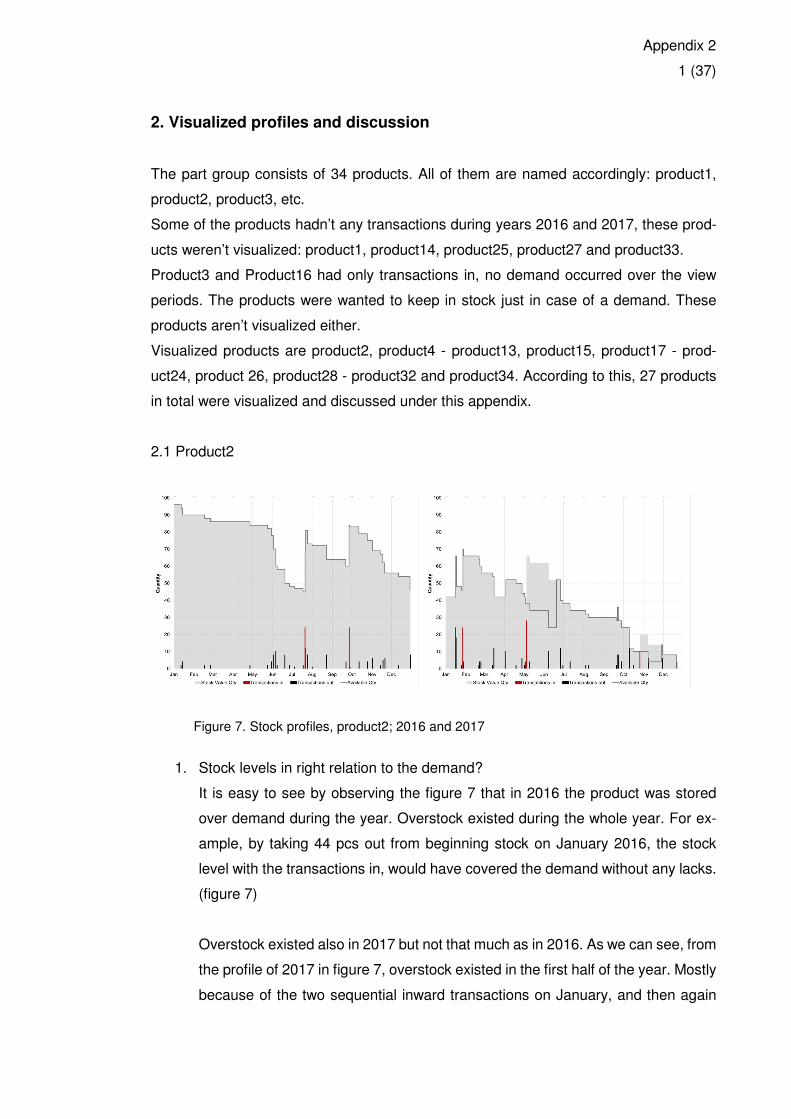
Appendix 2
1 (37)
2. Visualized profiles and discussion
The part group consists of 34 products. All of them are named accordingly: product1,
product2, product3, etc.
Some of the products hadn’t any transactions during years 2016 and 2017, these prod-
ucts weren’t visualized: product1, product14, product25, product27 and product33.
Product3 and Product16 had only transactions in, no demand occurred over the view
periods. The products were wanted to keep in stock just in case of a demand. These
products aren’t visualized either.
Visualized products are product2, product4 - product13, product15, product17 - prod-
uct24, product 26, product28 - product32 and product34. According to this, 27 products
in total were visualized and discussed under this appendix.
2.1 Product2
Figure 7. Stock profiles, product2; 2016 and 2017
1. Stock levels in right relation to the demand?
It is easy to see by observing the figure 7 that in 2016 the product was stored
over demand during the year. Overstock existed during the whole year. For ex-
ample, by taking 44 pcs out from beginning stock on January 2016, the stock
level with the transactions in, would have covered the demand without any lacks.
(figure 7)
Overstock existed also in 2017 but not that much as in 2016. As we can see, from
the profile of 2017 in figure 7, overstock existed in the first half of the year. Mostly
because of the two sequential inward transactions on January, and then again
Appendix 2
2 (37)
on April and May. In the end of the 2017 the stock level was surprisingly low and
stock required supplement. (figure 7)
In 2016 the nature of demand of Product2 was intermittent and lumpy. Forecast-
ing the future demand for stock controlling purposes is challenging. In 2016, the
transaction out happened 27 times and the product quantity per transaction out
was between one to ten pieces. Until June 2016, there were a lot less demand
than the rest of the year. The demand of 2016 was 110 pieces. 98 pieces oc-
curred from June 2016. (figure 7)
In 2017, the situation was completely changed. At that time, the demand occurred
on monthly basis. However, the product quantity per transaction out was more
varied than a year earlier. During August 2017, the demand was on lowest and
the next transactions out happened not until the end of September. In 2017, the
transaction out happened 27 times and the product quantity per transaction out
was between 2 to 18 pieces. The demand of 2017 was totally 142 pieces, com-
pared to 2016 it increased by 32 pcs. (figure 7)
Of course afterwards, it is quite easy to analyse transactions and make conclu-
sions of how the stock planning should have been done. If the demand is not
steady, as it wasn’t in this case, you have to prepare for intermittent and variable
demand. Prepare by holding stock, stock levels based on forecasted demand.
2. Right amount purchased?
In 2016 transactions in held 60 pieces of products. As mentioned before, by tak-
ing 44 pieces out from the beginning stock in 2016, existing stock with the trans-
action in would have covered the demand. On the other hand, there were three
transactions in holding 24, 12 and 24 pieces of the product. One transaction in
holding 24 pcs would have covered the whole demand of 2016. (figure 7)
In 2017 transactions in was holding totally 104 pieces of the product. What comes
to the demand of the year, 104 pieces was a right amount to be purchased to
cover the demand. While, the timing and the order amounts wasn’t. Shortly, too
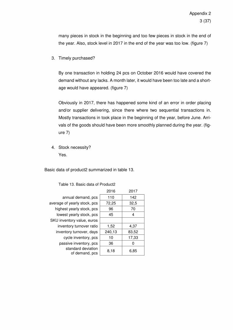
Appendix 2
3 (37)
many pieces in stock in the beginning and too few pieces in stock in the end of
the year. Also, stock level in 2017 in the end of the year was too low. (figure 7)
3. Timely purchased?
By one transaction in holding 24 pcs on October 2016 would have covered the
demand without any lacks. A month later, it would have been too late and a short-
age would have appeared. (figure 7)
Obviously in 2017, there has happened some kind of an error in order placing
and/or supplier delivering, since there where two sequential transactions in.
Mostly transactions in took place in the beginning of the year, before June. Arri-
vals of the goods should have been more smoothly planned during the year. (fig-
ure 7)
4. Stock necessity?
Yes.
Basic data of product2 summarized in table 13.
Table 13. Basic data of Product2
2016 2017
annual demand, pcs 110 142
average of yearly stock, pcs 72,25 32,5
highest yearly stock, pcs 96 70
lowest yearly stock, pcs 45 4
SKU inventory value, euros
inventory turnover ratio 1,52 4,37
inventory turnover, days 240,13 83,52
cycle inventory, pcs 10 17,33
passive inventory, pcs 36 0
standard deviation of demand, pcs
8,18 6,85
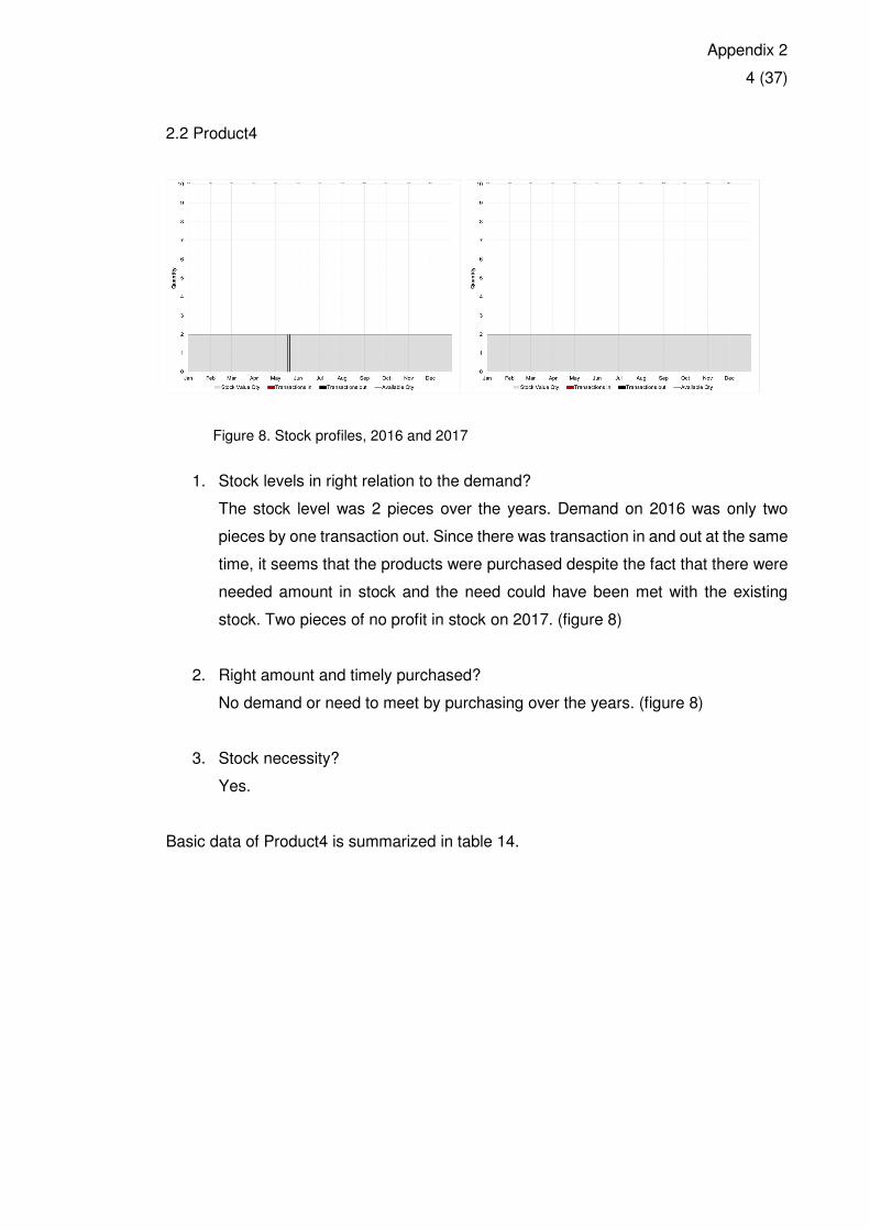
Appendix 2
4 (37)
2.2 Product4
Figure 8. Stock profiles, 2016 and 2017
1. Stock levels in right relation to the demand?
The stock level was 2 pieces over the years. Demand on 2016 was only two
pieces by one transaction out. Since there was transaction in and out at the same
time, it seems that the products were purchased despite the fact that there were
needed amount in stock and the need could have been met with the existing
stock. Two pieces of no profit in stock on 2017. (figure 8)
2. Right amount and timely purchased?
No demand or need to meet by purchasing over the years. (figure 8)
3. Stock necessity?
Yes.
Basic data of Product4 is summarized in table 14.
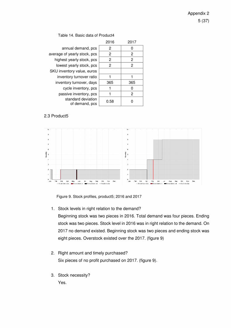
Appendix 2
5 (37)
Table 14. Basic data of Product4
2016 2017
annual demand, pcs 2 0
average of yearly stock, pcs 2 2
highest yearly stock, pcs 2 2
lowest yearly stock, pcs 2 2
SKU inventory value, euros
inventory turnover ratio 1 1
inventory turnover, days 365 365
cycle inventory, pcs 1 0
passive inventory, pcs 1 2
standard deviation of demand, pcs
0.58 0
2.3 Product5
Figure 9. Stock profiles, product5; 2016 and 2017
1. Stock levels in right relation to the demand?
Beginning stock was two pieces in 2016. Total demand was four pieces. Ending
stock was two pieces. Stock level in 2016 was in right relation to the demand. On
2017 no demand existed. Beginning stock was two pieces and ending stock was
eight pieces. Overstock existed over the 2017. (figure 9)
2. Right amount and timely purchased?
Six pieces of no profit purchased on 2017. (figure 9).
3. Stock necessity?
Yes.
Appendix 2
6 (37)
Basic data of Product5 summarized in table 15.
Table 15. Basic data of Product5
2016 2017
annual demand, pcs 4 0
average of yearly stock, pcs 1,83 6,25
highest yearly stock, pcs 2 8
lowest yearly stock, pcs 0 2
SKU inventory value, euros
inventory turnover ratio 2,19 0
inventory turnover, days 166,67 365
cycle inventory, pcs 1 1,5
passive inventory, pcs 1 6,5
standard deviation of demand, pcs
0,78 -
2.4 Product6
Figure 10. Stock profile, product6; 2016
1. Stock levels in right relation to the demand?
Beginning stock was one piece in 2016. Only one transaction out on November
2016, no stock held afterwards. Stock level was in right relation to the demand.
(figure 10)
2. Right amount and timely purchased?
No purchases during 2016 or 2017. (figure 10)
3. Stock necessity?
Yes.
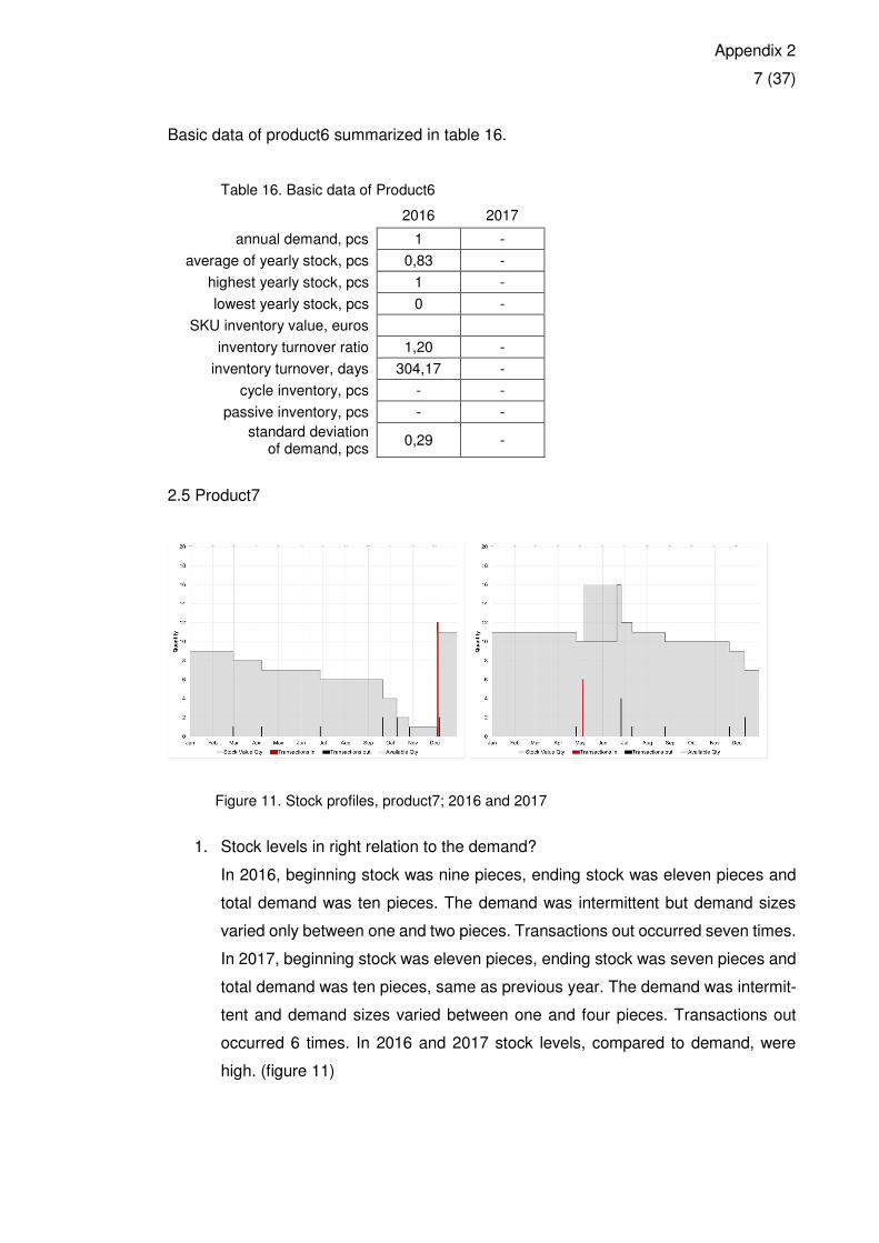
Appendix 2
7 (37)
Basic data of product6 summarized in table 16.
Table 16. Basic data of Product6
2016 2017
annual demand, pcs 1 -
average of yearly stock, pcs 0,83 -
highest yearly stock, pcs 1 -
lowest yearly stock, pcs 0 -
SKU inventory value, euros
inventory turnover ratio 1,20 -
inventory turnover, days 304,17 -
cycle inventory, pcs - -
passive inventory, pcs - -
standard deviation of demand, pcs
0,29 -
2.5 Product7
Figure 11. Stock profiles, product7; 2016 and 2017
1. Stock levels in right relation to the demand?
In 2016, beginning stock was nine pieces, ending stock was eleven pieces and
total demand was ten pieces. The demand was intermittent but demand sizes
varied only between one and two pieces. Transactions out occurred seven times.
In 2017, beginning stock was eleven pieces, ending stock was seven pieces and
total demand was ten pieces, same as previous year. The demand was intermit-
tent and demand sizes varied between one and four pieces. Transactions out
occurred 6 times. In 2016 and 2017 stock levels, compared to demand, were
high. (figure 11)
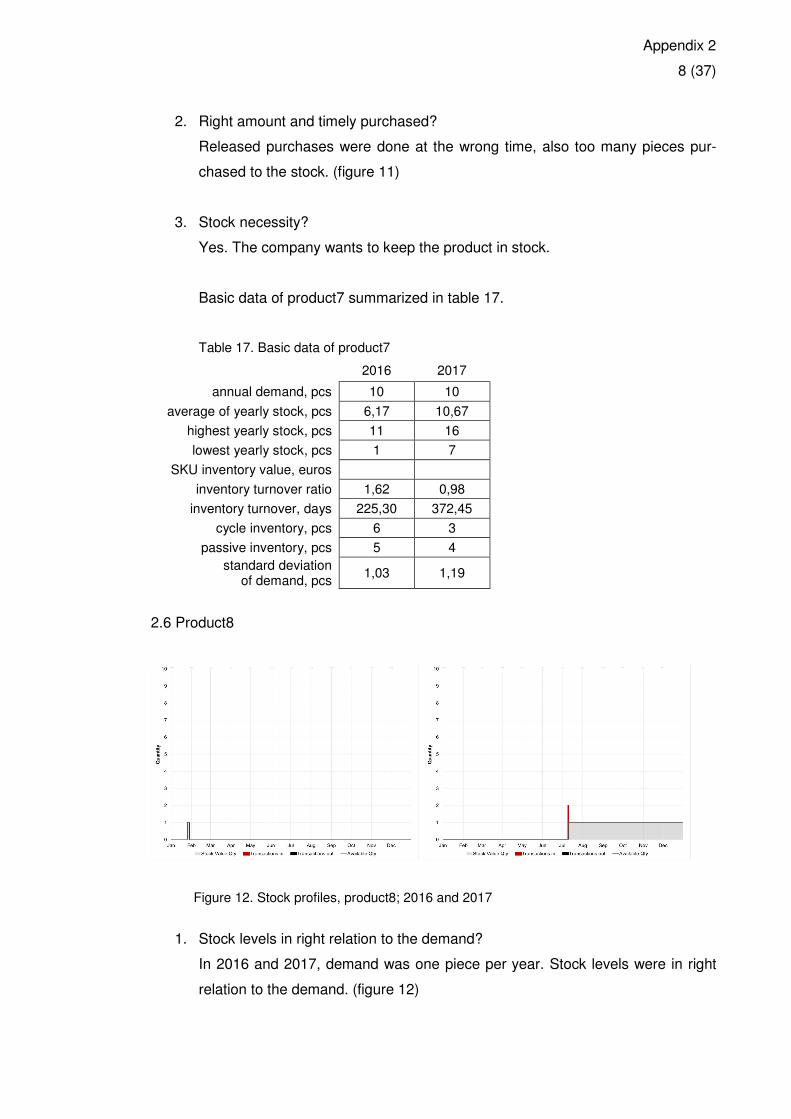
Appendix 2
8 (37)
2. Right amount and timely purchased?
Released purchases were done at the wrong time, also too many pieces pur-
chased to the stock. (figure 11)
3. Stock necessity?
Yes. The company wants to keep the product in stock.
Basic data of product7 summarized in table 17.
Table 17. Basic data of product7
2016 2017
annual demand, pcs 10 10
average of yearly stock, pcs 6,17 10,67
highest yearly stock, pcs 11 16
lowest yearly stock, pcs 1 7
SKU inventory value, euros
inventory turnover ratio 1,62 0,98
inventory turnover, days 225,30 372,45
cycle inventory, pcs 6 3
passive inventory, pcs 5 4
standard deviation of demand, pcs
1,03 1,19
2.6 Product8
Figure 12. Stock profiles, product8; 2016 and 2017
1. Stock levels in right relation to the demand?
In 2016 and 2017, demand was one piece per year. Stock levels were in right
relation to the demand. (figure 12)
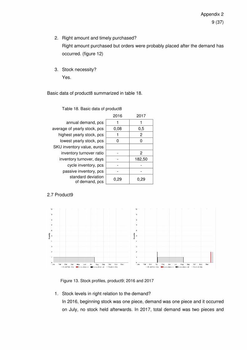
Appendix 2
9 (37)
2. Right amount and timely purchased?
Right amount purchased but orders were probably placed after the demand has
occurred. (figure 12)
3. Stock necessity?
Yes.
Basic data of product8 summarized in table 18.
Table 18. Basic data of product8
2016 2017
annual demand, pcs 1 1
average of yearly stock, pcs 0,08 0,5
highest yearly stock, pcs 1 2
lowest yearly stock, pcs 0 0
SKU inventory value, euros
inventory turnover ratio - 2
inventory turnover, days - 182,50
cycle inventory, pcs - -
passive inventory, pcs - -
standard deviation of demand, pcs
0,29 0,29
2.7 Product9
Figure 13. Stock profiles, product9; 2016 and 2017
1. Stock levels in right relation to the demand?
In 2016, beginning stock was one piece, demand was one piece and it occurred
on July, no stock held afterwards. In 2017, total demand was two pieces and
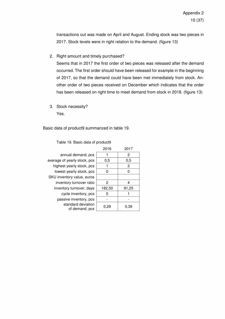
Appendix 2
10 (37)
transactions out was made on April and August. Ending stock was two pieces in
2017. Stock levels were in right relation to the demand. (figure 13)
2. Right amount and timely purchased?
Seems that in 2017 the first order of two pieces was released after the demand
occurred. The first order should have been released for example in the beginning
of 2017, so that the demand could have been met immediately from stock. An-
other order of two pieces received on December which indicates that the order
has been released on right time to meet demand from stock in 2018. (figure 13)
3. Stock necessity?
Yes.
Basic data of product9 summarized in table 19.
Table 19. Basic data of product9
2016 2017
annual demand, pcs 1 2
average of yearly stock, pcs 0,5 0,5
highest yearly stock, pcs 1 2
lowest yearly stock, pcs 0 0
SKU inventory value, euros
inventory turnover ratio 2 4
inventory turnover, days 182,50 91,25
cycle inventory, pcs 0 1
passive inventory, pcs - -
standard deviation of demand, pcs
0,29 0,39
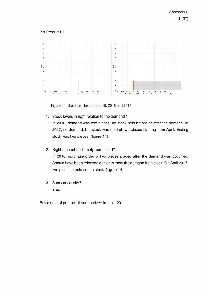
Appendix 2
11 (37)
2.8 Product10
Figure 14. Stock profiles, product10; 2016 and 2017
1. Stock levels in right relation to the demand?
In 2016, demand was two pieces, no stock held before or after the demand. In
2017, no demand, but stock was held of two pieces starting from April. Ending
stock was two pieces. (figure 14)
2. Right amount and timely purchased?
In 2016, purchase order of two pieces placed after the demand was occurred.
Should have been released earlier to meet the demand from stock. On April 2017,
two pieces purchased to stock. (figure 14)
3. Stock necessity?
Yes.
Basic data of product10 summarized in table 20.
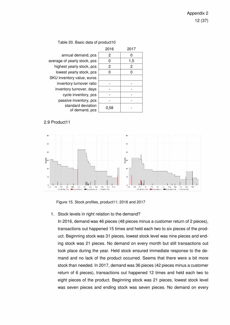
Appendix 2
12 (37)
Table 20. Basic data of product10
2016 2017
annual demand, pcs 2 0
average of yearly stock, pcs 0 1,5
highest yearly stock, pcs 2 2
lowest yearly stock, pcs 0 0
SKU inventory value, euros
inventory turnover ratio - -
inventory turnover, days - -
cycle inventory, pcs - -
passive inventory, pcs - -
standard deviation of demand, pcs
0,58 -
2.9 Product11
Figure 15. Stock profiles, product11; 2016 and 2017
1. Stock levels in right relation to the demand?
In 2016, demand was 46 pieces (48 pieces minus a customer return of 2 pieces),
transactions out happened 15 times and held each two to six pieces of the prod-
uct. Beginning stock was 31 pieces, lowest stock level was nine pieces and end-
ing stock was 21 pieces. No demand on every month but still transactions out
took place during the year. Held stock ensured immediate response to the de-
mand and no lack of the product occurred. Seems that there were a bit more
stock than needed. In 2017, demand was 36 pieces (42 pieces minus a customer
return of 6 pieces), transactions out happened 12 times and held each two to
eight pieces of the product. Beginning stock was 21 pieces, lowest stock level
was seven pieces and ending stock was seven pieces. No demand on every
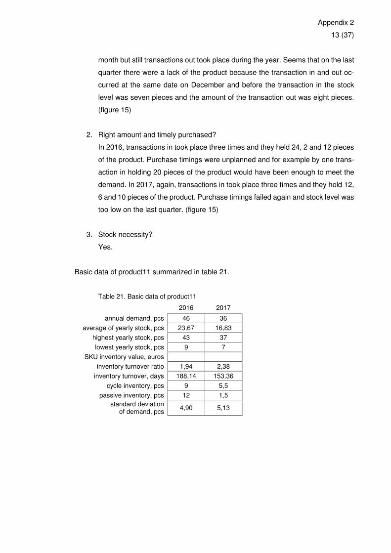
Appendix 2
13 (37)
month but still transactions out took place during the year. Seems that on the last
quarter there were a lack of the product because the transaction in and out oc-
curred at the same date on December and before the transaction in the stock
level was seven pieces and the amount of the transaction out was eight pieces.
(figure 15)
2. Right amount and timely purchased?
In 2016, transactions in took place three times and they held 24, 2 and 12 pieces
of the product. Purchase timings were unplanned and for example by one trans-
action in holding 20 pieces of the product would have been enough to meet the
demand. In 2017, again, transactions in took place three times and they held 12,
6 and 10 pieces of the product. Purchase timings failed again and stock level was
too low on the last quarter. (figure 15)
3. Stock necessity?
Yes.
Basic data of product11 summarized in table 21.
Table 21. Basic data of product11
2016 2017
annual demand, pcs 46 36
average of yearly stock, pcs 23,67 16,83
highest yearly stock, pcs 43 37
lowest yearly stock, pcs 9 7
SKU inventory value, euros
inventory turnover ratio 1,94 2,38
inventory turnover, days 188,14 153,36
cycle inventory, pcs 9 5,5
passive inventory, pcs 12 1,5
standard deviation of demand, pcs
4,90 5,13
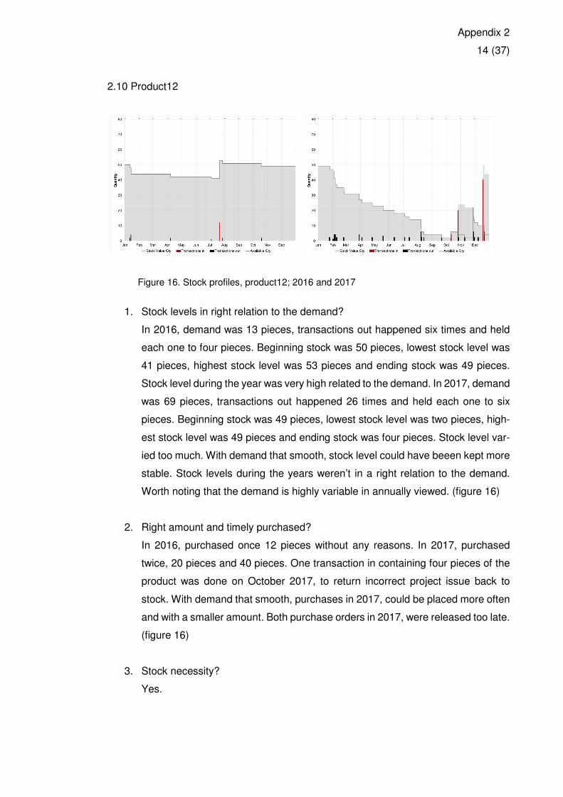
Appendix 2
14 (37)
2.10 Product12
Figure 16. Stock profiles, product12; 2016 and 2017
1. Stock levels in right relation to the demand?
In 2016, demand was 13 pieces, transactions out happened six times and held
each one to four pieces. Beginning stock was 50 pieces, lowest stock level was
41 pieces, highest stock level was 53 pieces and ending stock was 49 pieces.
Stock level during the year was very high related to the demand. In 2017, demand
was 69 pieces, transactions out happened 26 times and held each one to six
pieces. Beginning stock was 49 pieces, lowest stock level was two pieces, high-
est stock level was 49 pieces and ending stock was four pieces. Stock level var-
ied too much. With demand that smooth, stock level could have beeen kept more
stable. Stock levels during the years weren’t in a right relation to the demand.
Worth noting that the demand is highly variable in annually viewed. (figure 16)
2. Right amount and timely purchased?
In 2016, purchased once 12 pieces without any reasons. In 2017, purchased
twice, 20 pieces and 40 pieces. One transaction in containing four pieces of the
product was done on October 2017, to return incorrect project issue back to
stock. With demand that smooth, purchases in 2017, could be placed more often
and with a smaller amount. Both purchase orders in 2017, were released too late.
(figure 16)
3. Stock necessity?
Yes.
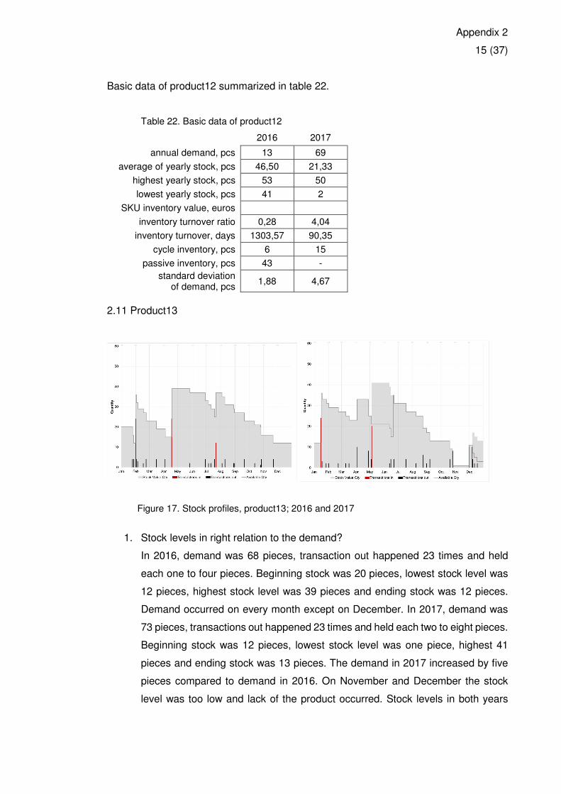
Appendix 2
15 (37)
Basic data of product12 summarized in table 22.
Table 22. Basic data of product12
2016 2017
annual demand, pcs 13 69
average of yearly stock, pcs 46,50 21,33
highest yearly stock, pcs 53 50
lowest yearly stock, pcs 41 2
SKU inventory value, euros
inventory turnover ratio 0,28 4,04
inventory turnover, days 1303,57 90,35
cycle inventory, pcs 6 15
passive inventory, pcs 43 -
standard deviation of demand, pcs
1,88 4,67
2.11 Product13
Figure 17. Stock profiles, product13; 2016 and 2017
1. Stock levels in right relation to the demand?
In 2016, demand was 68 pieces, transaction out happened 23 times and held
each one to four pieces. Beginning stock was 20 pieces, lowest stock level was
12 pieces, highest stock level was 39 pieces and ending stock was 12 pieces.
Demand occurred on every month except on December. In 2017, demand was
73 pieces, transactions out happened 23 times and held each two to eight pieces.
Beginning stock was 12 pieces, lowest stock level was one piece, highest 41
pieces and ending stock was 13 pieces. The demand in 2017 increased by five
pieces compared to demand in 2016. On November and December the stock
level was too low and lack of the product occurred. Stock levels in both years
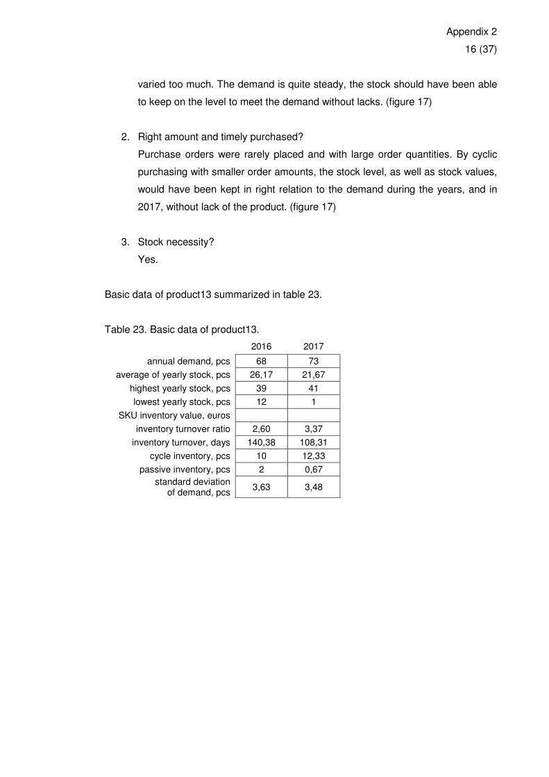
Appendix 2
16 (37)
varied too much. The demand is quite steady, the stock should have been able
to keep on the level to meet the demand without lacks. (figure 17)
2. Right amount and timely purchased?
Purchase orders were rarely placed and with large order quantities. By cyclic
purchasing with smaller order amounts, the stock level, as well as stock values,
would have been kept in right relation to the demand during the years, and in
2017, without lack of the product. (figure 17)
3. Stock necessity?
Yes.
Basic data of product13 summarized in table 23.
Table 23. Basic data of product13.
2016 2017
annual demand, pcs 68 73
average of yearly stock, pcs 26,17 21,67
highest yearly stock, pcs 39 41
lowest yearly stock, pcs 12 1
SKU inventory value, euros
inventory turnover ratio 2,60 3,37
inventory turnover, days 140,38 108,31
cycle inventory, pcs 10 12,33
passive inventory, pcs 2 0,67
standard deviation of demand, pcs
3,63 3,48
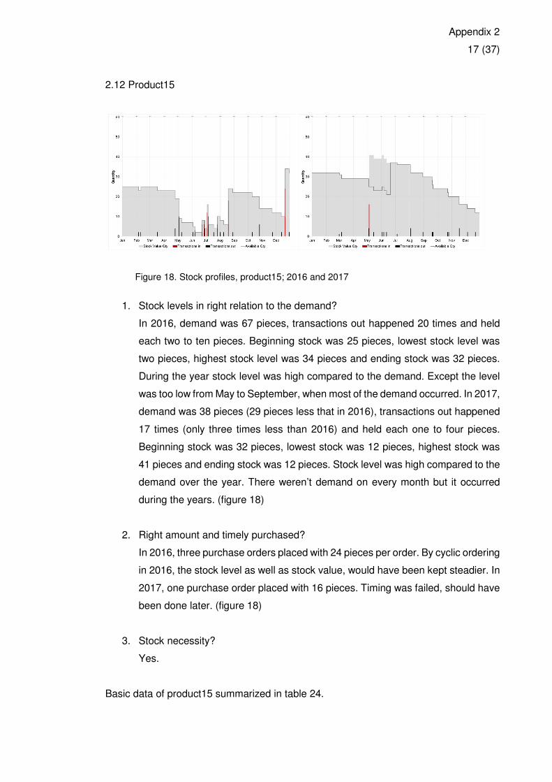
Appendix 2
17 (37)
2.12 Product15
Figure 18. Stock profiles, product15; 2016 and 2017
1. Stock levels in right relation to the demand?
In 2016, demand was 67 pieces, transactions out happened 20 times and held
each two to ten pieces. Beginning stock was 25 pieces, lowest stock level was
two pieces, highest stock level was 34 pieces and ending stock was 32 pieces.
During the year stock level was high compared to the demand. Except the level
was too low from May to September, when most of the demand occurred. In 2017,
demand was 38 pieces (29 pieces less that in 2016), transactions out happened
17 times (only three times less than 2016) and held each one to four pieces.
Beginning stock was 32 pieces, lowest stock was 12 pieces, highest stock was
41 pieces and ending stock was 12 pieces. Stock level was high compared to the
demand over the year. There weren’t demand on every month but it occurred
during the years. (figure 18)
2. Right amount and timely purchased?
In 2016, three purchase orders placed with 24 pieces per order. By cyclic ordering
in 2016, the stock level as well as stock value, would have been kept steadier. In
2017, one purchase order placed with 16 pieces. Timing was failed, should have
been done later. (figure 18)
3. Stock necessity?
Yes.
Basic data of product15 summarized in table 24.
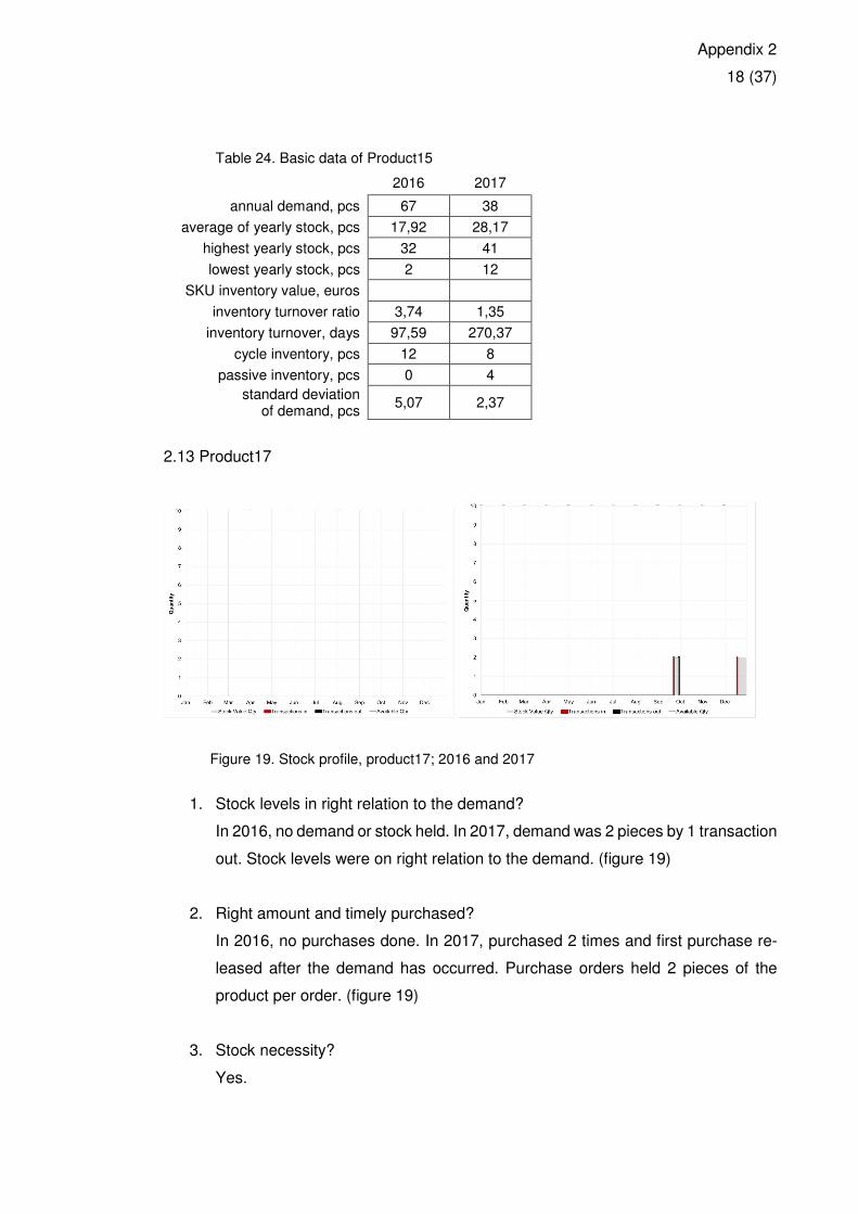
Appendix 2
18 (37)
Table 24. Basic data of Product15
2016 2017
annual demand, pcs 67 38
average of yearly stock, pcs 17,92 28,17
highest yearly stock, pcs 32 41
lowest yearly stock, pcs 2 12
SKU inventory value, euros
inventory turnover ratio 3,74 1,35
inventory turnover, days 97,59 270,37
cycle inventory, pcs 12 8
passive inventory, pcs 0 4
standard deviation of demand, pcs
5,07 2,37
2.13 Product17
Figure 19. Stock profile, product17; 2016 and 2017
1. Stock levels in right relation to the demand?
In 2016, no demand or stock held. In 2017, demand was 2 pieces by 1 transaction
out. Stock levels were on right relation to the demand. (figure 19)
2. Right amount and timely purchased?
In 2016, no purchases done. In 2017, purchased 2 times and first purchase re-
leased after the demand has occurred. Purchase orders held 2 pieces of the
product per order. (figure 19)
3. Stock necessity?
Yes.
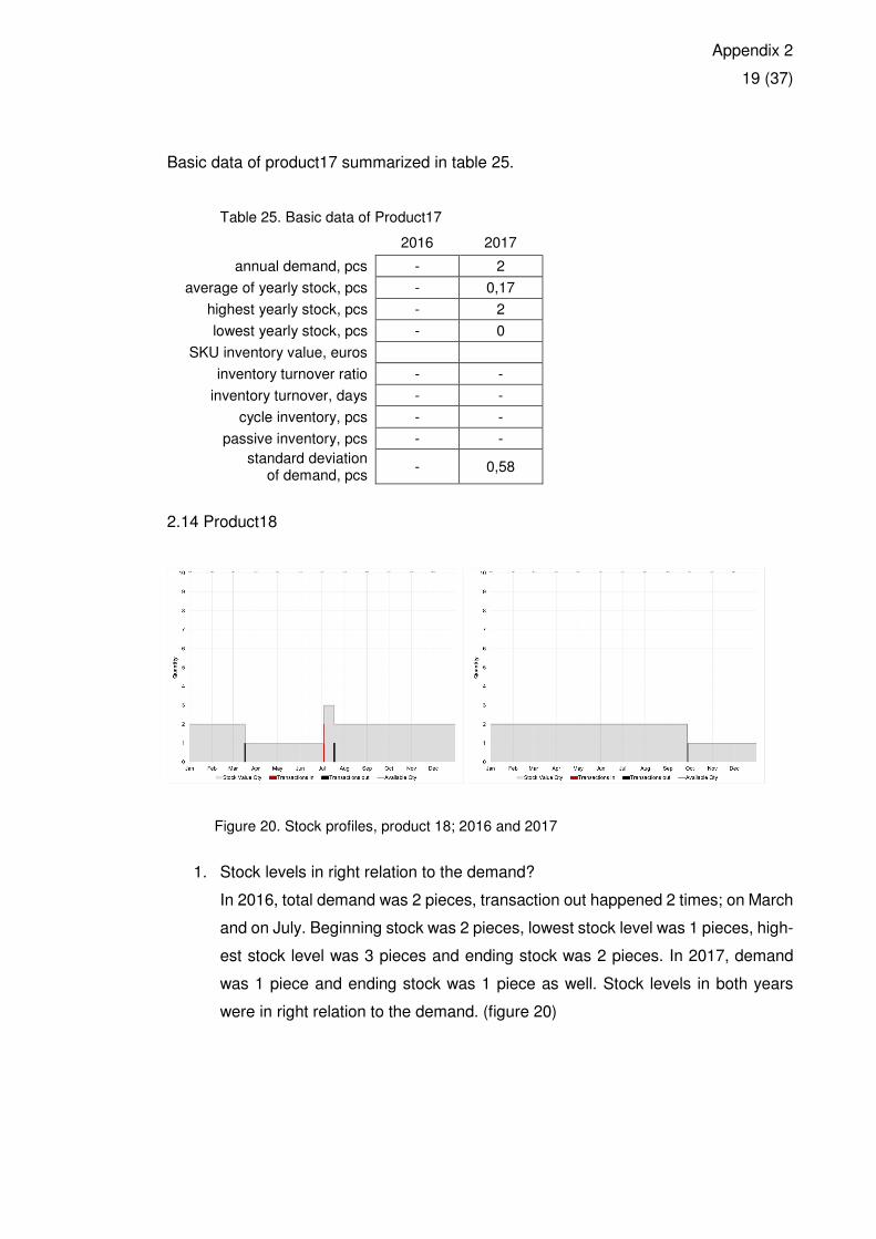
Appendix 2
19 (37)
Basic data of product17 summarized in table 25.
Table 25. Basic data of Product17
2016 2017
annual demand, pcs - 2
average of yearly stock, pcs - 0,17
highest yearly stock, pcs - 2
lowest yearly stock, pcs - 0
SKU inventory value, euros
inventory turnover ratio - -
inventory turnover, days - -
cycle inventory, pcs - -
passive inventory, pcs - -
standard deviation of demand, pcs
- 0,58
2.14 Product18
Figure 20. Stock profiles, product 18; 2016 and 2017
1. Stock levels in right relation to the demand?
In 2016, total demand was 2 pieces, transaction out happened 2 times; on March
and on July. Beginning stock was 2 pieces, lowest stock level was 1 pieces, high-
est stock level was 3 pieces and ending stock was 2 pieces. In 2017, demand
was 1 piece and ending stock was 1 piece as well. Stock levels in both years
were in right relation to the demand. (figure 20)
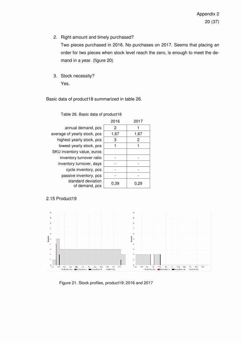
Appendix 2
20 (37)
2. Right amount and timely purchased?
Two pieces purchased in 2016. No purchases on 2017. Seems that placing an
order for two pieces when stock level reach the zero, is enough to meet the de-
mand in a year. (figure 20)
3. Stock necessity?
Yes.
Basic data of product18 summarized in table 26.
Table 26. Basic data of product18
2016 2017
annual demand, pcs 2 1
average of yearly stock, pcs 1,67 1,67
highest yearly stock, pcs 3 2
lowest yearly stock, pcs 1 1
SKU inventory value, euros
inventory turnover ratio - -
inventory turnover, days - -
cycle inventory, pcs - -
passive inventory, pcs - -
standard deviation of demand, pcs
0,39 0,29
2.15 Product19
Figure 21. Stock profiles, product19; 2016 and 2017
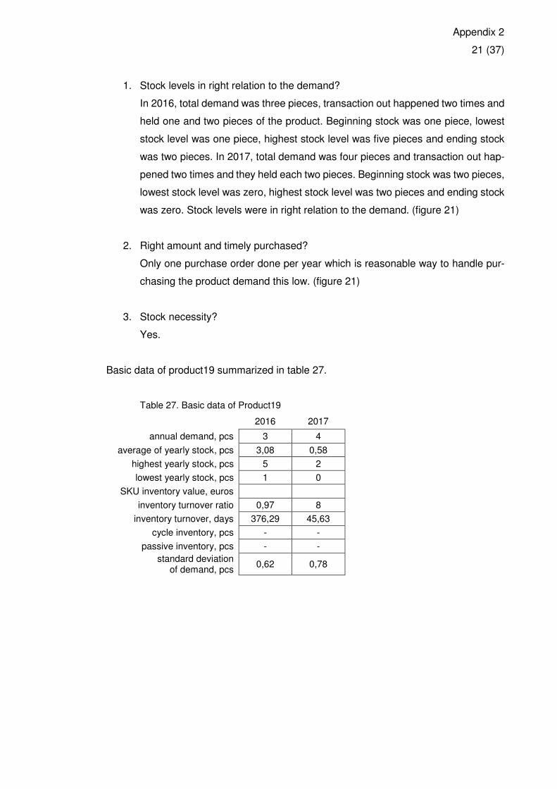
Appendix 2
21 (37)
1. Stock levels in right relation to the demand?
In 2016, total demand was three pieces, transaction out happened two times and
held one and two pieces of the product. Beginning stock was one piece, lowest
stock level was one piece, highest stock level was five pieces and ending stock
was two pieces. In 2017, total demand was four pieces and transaction out hap-
pened two times and they held each two pieces. Beginning stock was two pieces,
lowest stock level was zero, highest stock level was two pieces and ending stock
was zero. Stock levels were in right relation to the demand. (figure 21)
2. Right amount and timely purchased?
Only one purchase order done per year which is reasonable way to handle pur-
chasing the product demand this low. (figure 21)
3. Stock necessity?
Yes.
Basic data of product19 summarized in table 27.
Table 27. Basic data of Product19
2016 2017
annual demand, pcs 3 4
average of yearly stock, pcs 3,08 0,58
highest yearly stock, pcs 5 2
lowest yearly stock, pcs 1 0
SKU inventory value, euros
inventory turnover ratio 0,97 8
inventory turnover, days 376,29 45,63
cycle inventory, pcs - -
passive inventory, pcs - -
standard deviation of demand, pcs
0,62 0,78
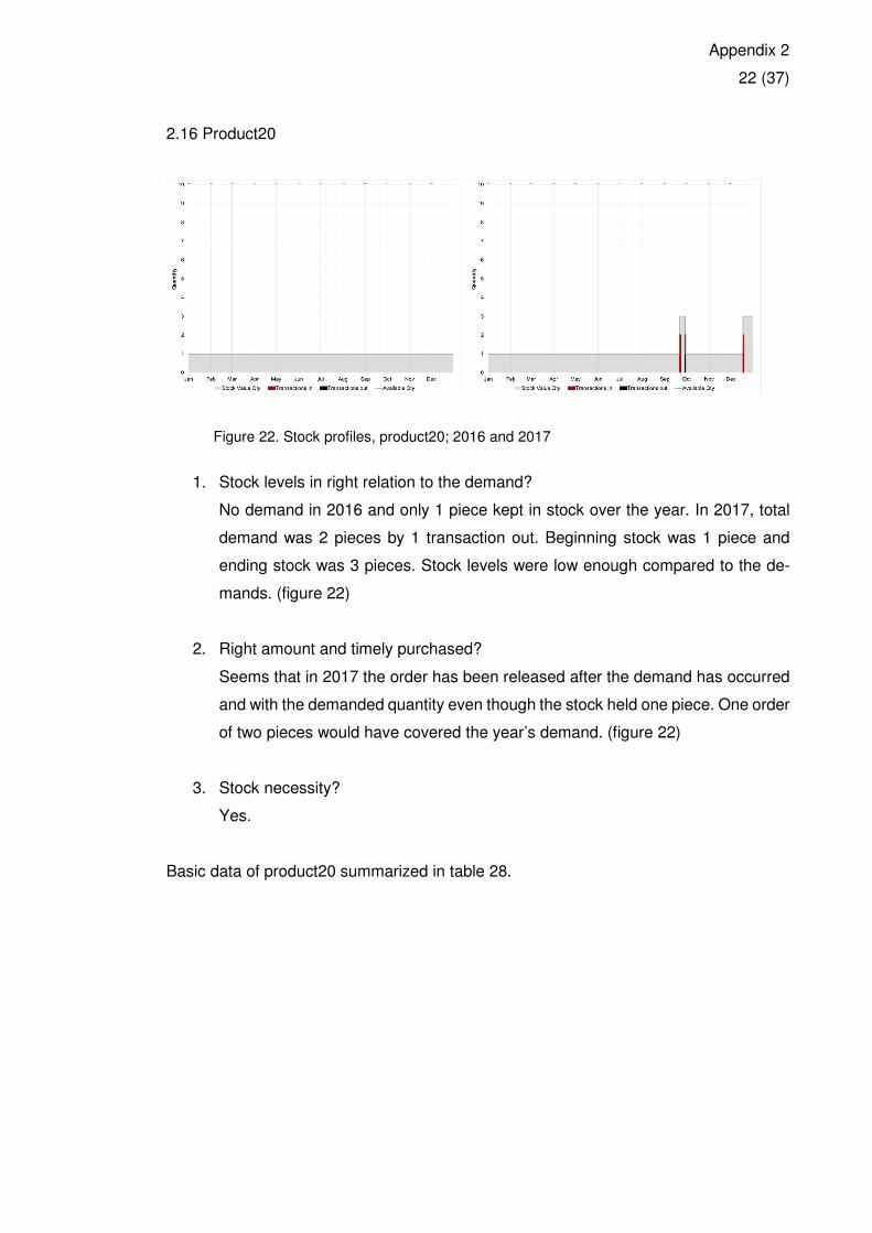
Appendix 2
22 (37)
2.16 Product20
Figure 22. Stock profiles, product20; 2016 and 2017
1. Stock levels in right relation to the demand?
No demand in 2016 and only 1 piece kept in stock over the year. In 2017, total
demand was 2 pieces by 1 transaction out. Beginning stock was 1 piece and
ending stock was 3 pieces. Stock levels were low enough compared to the de-
mands. (figure 22)
2. Right amount and timely purchased?
Seems that in 2017 the order has been released after the demand has occurred
and with the demanded quantity even though the stock held one piece. One order
of two pieces would have covered the year’s demand. (figure 22)
3. Stock necessity?
Yes.
Basic data of product20 summarized in table 28.
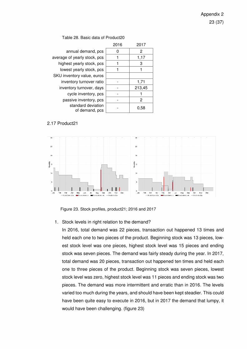
Appendix 2
23 (37)
Table 28. Basic data of Product20
2016 2017
annual demand, pcs 0 2
average of yearly stock, pcs 1 1,17
highest yearly stock, pcs 1 3
lowest yearly stock, pcs 1 1
SKU inventory value, euros
inventory turnover ratio - 1,71
inventory turnover, days - 213,45
cycle inventory, pcs - 1
passive inventory, pcs - 2
standard deviation of demand, pcs
- 0,58
2.17 Product21
Figure 23. Stock profiles, product21; 2016 and 2017
1. Stock levels in right relation to the demand?
In 2016, total demand was 22 pieces, transaction out happened 13 times and
held each one to two pieces of the product. Beginning stock was 13 pieces, low-
est stock level was one pieces, highest stock level was 15 pieces and ending
stock was seven pieces. The demand was fairly steady during the year. In 2017,
total demand was 20 pieces, transaction out happened ten times and held each
one to three pieces of the product. Beginning stock was seven pieces, lowest
stock level was zero, highest stock level was 11 pieces and ending stock was two
pieces. The demand was more intermittent and erratic than in 2016. The levels
varied too much during the years, and should have been kept steadier. This could
have been quite easy to execute in 2016, but in 2017 the demand that lumpy, it
would have been challenging. (figure 23)
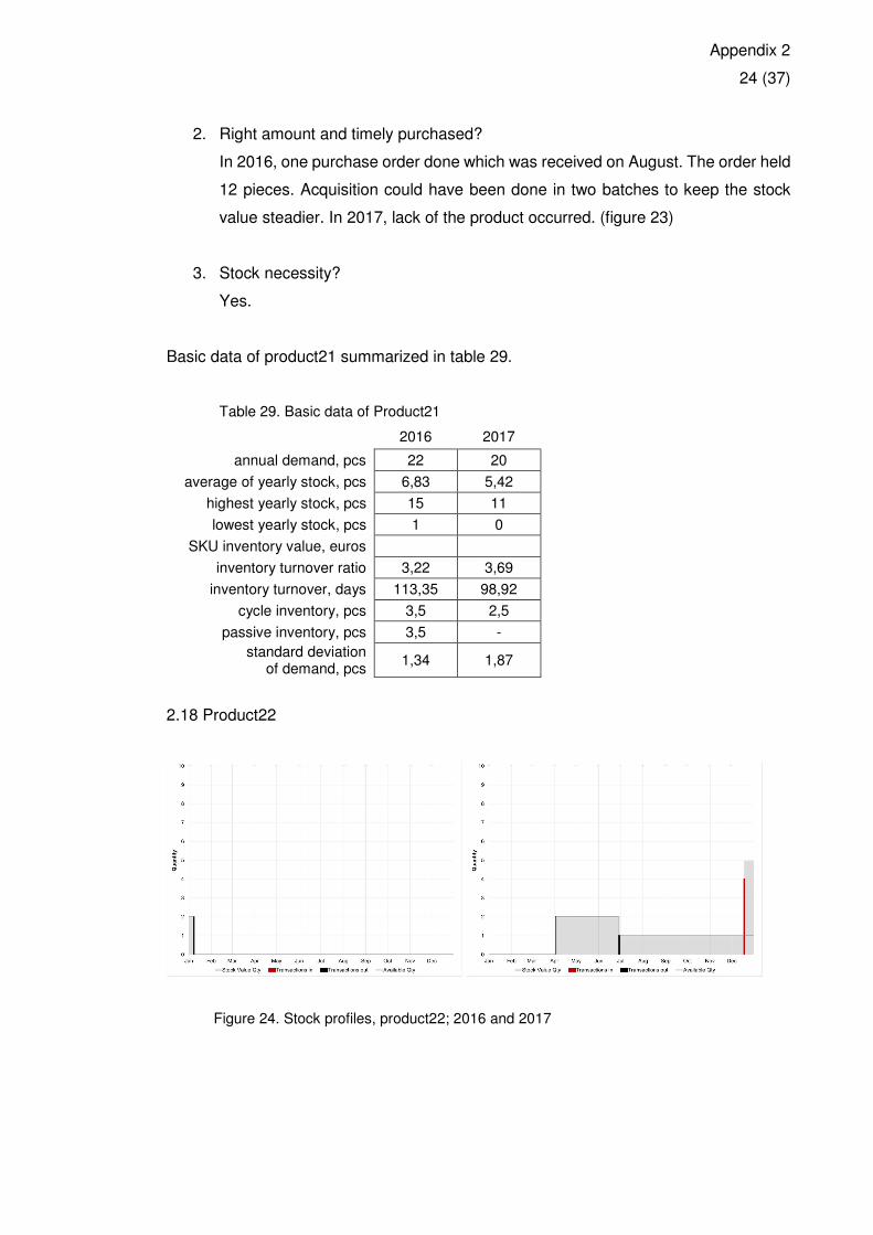
Appendix 2
24 (37)
2. Right amount and timely purchased?
In 2016, one purchase order done which was received on August. The order held
12 pieces. Acquisition could have been done in two batches to keep the stock
value steadier. In 2017, lack of the product occurred. (figure 23)
3. Stock necessity?
Yes.
Basic data of product21 summarized in table 29.
Table 29. Basic data of Product21
2016 2017
annual demand, pcs 22 20
average of yearly stock, pcs 6,83 5,42
highest yearly stock, pcs 15 11
lowest yearly stock, pcs 1 0
SKU inventory value, euros
inventory turnover ratio 3,22 3,69
inventory turnover, days 113,35 98,92
cycle inventory, pcs 3,5 2,5
passive inventory, pcs 3,5 -
standard deviation of demand, pcs
1,34 1,87
2.18 Product22
Figure 24. Stock profiles, product22; 2016 and 2017
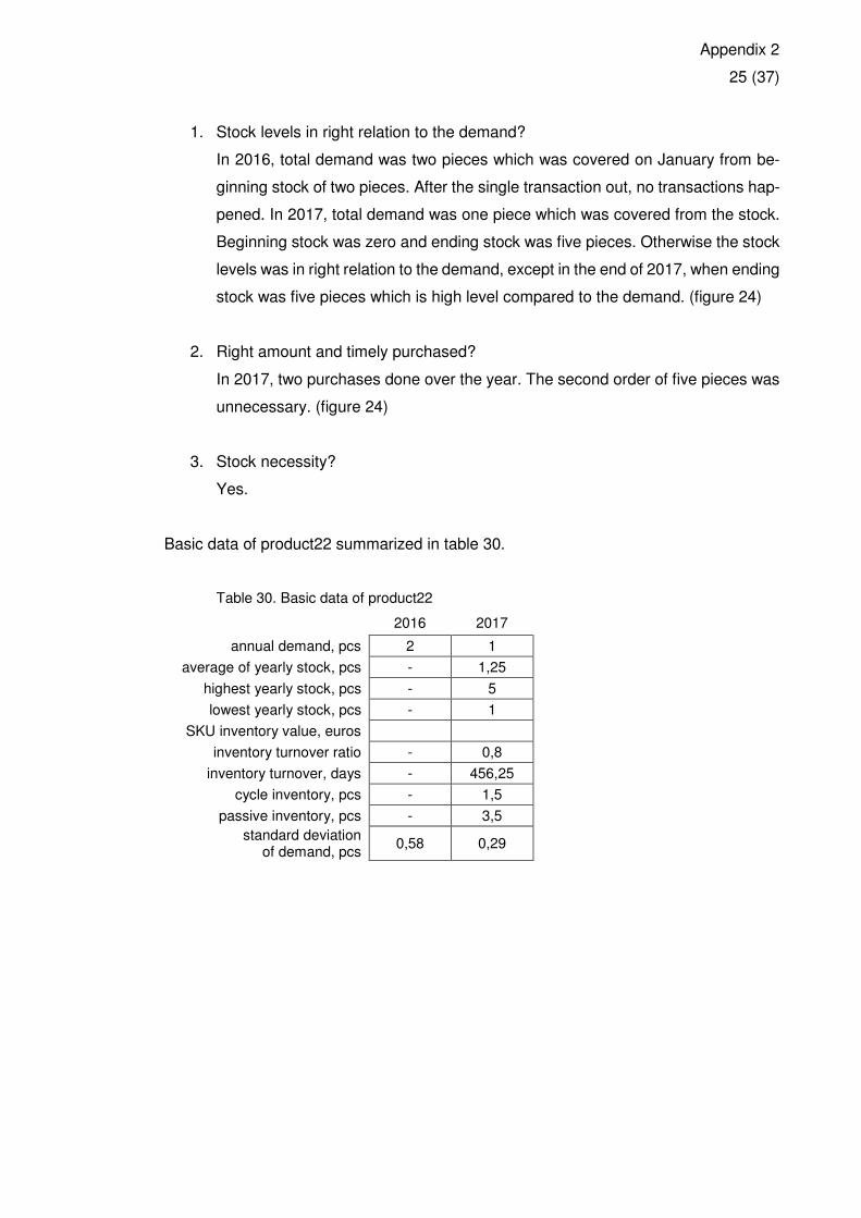
Appendix 2
25 (37)
1. Stock levels in right relation to the demand?
In 2016, total demand was two pieces which was covered on January from be-
ginning stock of two pieces. After the single transaction out, no transactions hap-
pened. In 2017, total demand was one piece which was covered from the stock.
Beginning stock was zero and ending stock was five pieces. Otherwise the stock
levels was in right relation to the demand, except in the end of 2017, when ending
stock was five pieces which is high level compared to the demand. (figure 24)
2. Right amount and timely purchased?
In 2017, two purchases done over the year. The second order of five pieces was
unnecessary. (figure 24)
3. Stock necessity?
Yes.
Basic data of product22 summarized in table 30.
Table 30. Basic data of product22
2016 2017
annual demand, pcs 2 1
average of yearly stock, pcs - 1,25
highest yearly stock, pcs - 5
lowest yearly stock, pcs - 1
SKU inventory value, euros
inventory turnover ratio - 0,8
inventory turnover, days - 456,25
cycle inventory, pcs - 1,5
passive inventory, pcs - 3,5
standard deviation of demand, pcs
0,58 0,29
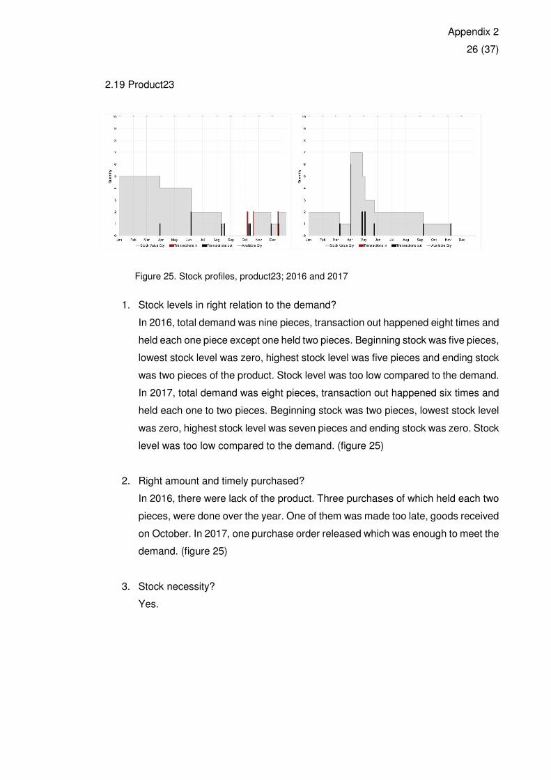
Appendix 2
26 (37)
2.19 Product23
Figure 25. Stock profiles, product23; 2016 and 2017
1. Stock levels in right relation to the demand?
In 2016, total demand was nine pieces, transaction out happened eight times and
held each one piece except one held two pieces. Beginning stock was five pieces,
lowest stock level was zero, highest stock level was five pieces and ending stock
was two pieces of the product. Stock level was too low compared to the demand.
In 2017, total demand was eight pieces, transaction out happened six times and
held each one to two pieces. Beginning stock was two pieces, lowest stock level
was zero, highest stock level was seven pieces and ending stock was zero. Stock
level was too low compared to the demand. (figure 25)
2. Right amount and timely purchased?
In 2016, there were lack of the product. Three purchases of which held each two
pieces, were done over the year. One of them was made too late, goods received
on October. In 2017, one purchase order released which was enough to meet the
demand. (figure 25)
3. Stock necessity?
Yes.
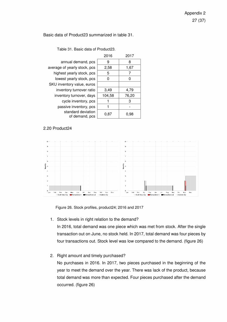
Appendix 2
27 (37)
Basic data of Product23 summarized in table 31.
Table 31. Basic data of Product23.
2016 2017
annual demand, pcs 9 8
average of yearly stock, pcs 2,58 1,67
highest yearly stock, pcs 5 7
lowest yearly stock, pcs 0 0
SKU inventory value, euros
inventory turnover ratio 3,49 4,79
inventory turnover, days 104,58 76,20
cycle inventory, pcs 1 3
passive inventory, pcs 1 -
standard deviation of demand, pcs
0,87 0,98
2.20 Product24
Figure 26. Stock profiles, product24; 2016 and 2017
1. Stock levels in right relation to the demand?
In 2016, total demand was one piece which was met from stock. After the single
transaction out on June, no stock held. In 2017, total demand was four pieces by
four transactions out. Stock level was low compared to the demand. (figure 26)
2. Right amount and timely purchased?
No purchases in 2016. In 2017, two pieces purchased in the beginning of the
year to meet the demand over the year. There was lack of the product, because
total demand was more than expected. Four pieces purchased after the demand
occurred. (figure 26)
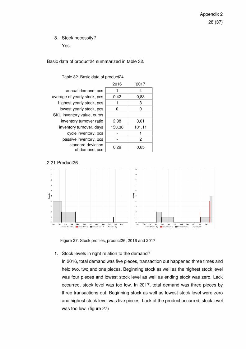
Appendix 2
28 (37)
3. Stock necessity?
Yes.
Basic data of product24 summarized in table 32.
Table 32. Basic data of product24
2016 2017
annual demand, pcs 1 4
average of yearly stock, pcs 0,42 0,83
highest yearly stock, pcs 1 3
lowest yearly stock, pcs 0 0
SKU inventory value, euros
inventory turnover ratio 2,38 3,61
inventory turnover, days 153,36 101,11
cycle inventory, pcs - 1
passive inventory, pcs - 2
standard deviation of demand, pcs
0,29 0,65
2.21 Product26
Figure 27. Stock profiles, product26; 2016 and 2017
1. Stock levels in right relation to the demand?
In 2016, total demand was five pieces, transaction out happened three times and
held two, two and one pieces. Beginning stock as well as the highest stock level
was four pieces and lowest stock level as well as ending stock was zero. Lack
occurred, stock level was too low. In 2017, total demand was three pieces by
three transactions out. Beginning stock as well as lowest stock level were zero
and highest stock level was five pieces. Lack of the product occurred, stock level
was too low. (figure 27)
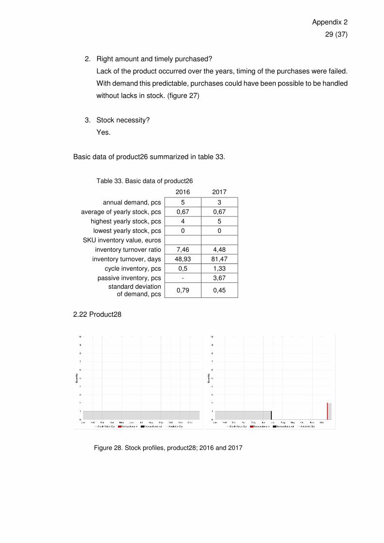
Appendix 2
29 (37)
2. Right amount and timely purchased?
Lack of the product occurred over the years, timing of the purchases were failed.
With demand this predictable, purchases could have been possible to be handled
without lacks in stock. (figure 27)
3. Stock necessity?
Yes.
Basic data of product26 summarized in table 33.
Table 33. Basic data of product26
2016 2017
annual demand, pcs 5 3
average of yearly stock, pcs 0,67 0,67
highest yearly stock, pcs 4 5
lowest yearly stock, pcs 0 0
SKU inventory value, euros
inventory turnover ratio 7,46 4,48
inventory turnover, days 48,93 81,47
cycle inventory, pcs 0,5 1,33
passive inventory, pcs - 3,67
standard deviation of demand, pcs
0,79 0,45
2.22 Product28
Figure 28. Stock profiles, product28; 2016 and 2017
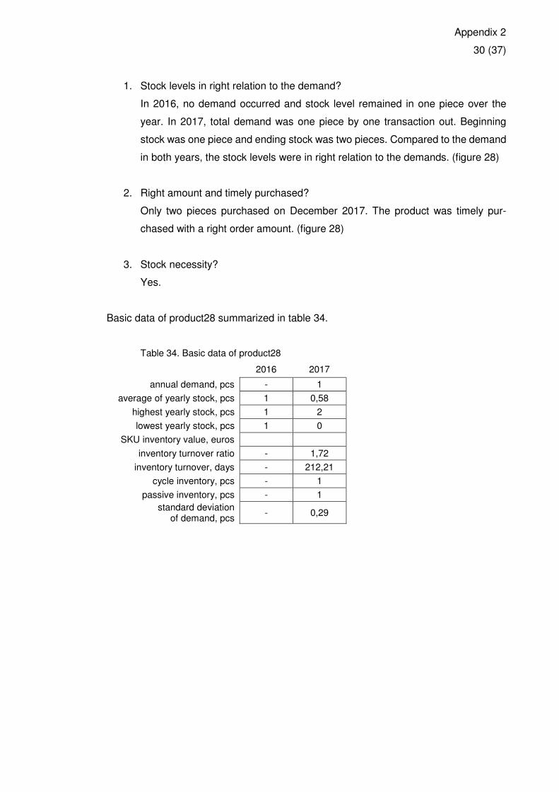
Appendix 2
30 (37)
1. Stock levels in right relation to the demand?
In 2016, no demand occurred and stock level remained in one piece over the
year. In 2017, total demand was one piece by one transaction out. Beginning
stock was one piece and ending stock was two pieces. Compared to the demand
in both years, the stock levels were in right relation to the demands. (figure 28)
2. Right amount and timely purchased?
Only two pieces purchased on December 2017. The product was timely pur-
chased with a right order amount. (figure 28)
3. Stock necessity?
Yes.
Basic data of product28 summarized in table 34.
Table 34. Basic data of product28
2016 2017
annual demand, pcs - 1
average of yearly stock, pcs 1 0,58
highest yearly stock, pcs 1 2
lowest yearly stock, pcs 1 0
SKU inventory value, euros
inventory turnover ratio - 1,72
inventory turnover, days - 212,21
cycle inventory, pcs - 1
passive inventory, pcs - 1
standard deviation of demand, pcs
- 0,29
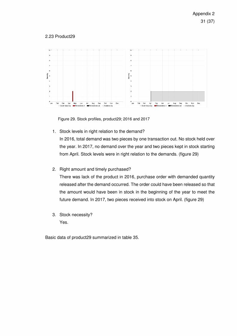
Appendix 2
31 (37)
2.23 Product29
Figure 29. Stock profiles, product29; 2016 and 2017
1. Stock levels in right relation to the demand?
In 2016, total demand was two pieces by one transaction out. No stock held over
the year. In 2017, no demand over the year and two pieces kept in stock starting
from April. Stock levels were in right relation to the demands. (figure 29)
2. Right amount and timely purchased?
There was lack of the product in 2016, purchase order with demanded quantity
released after the demand occurred. The order could have been released so that
the amount would have been in stock in the beginning of the year to meet the
future demand. In 2017, two pieces received into stock on April. (figure 29)
3. Stock necessity?
Yes.
Basic data of product29 summarized in table 35.
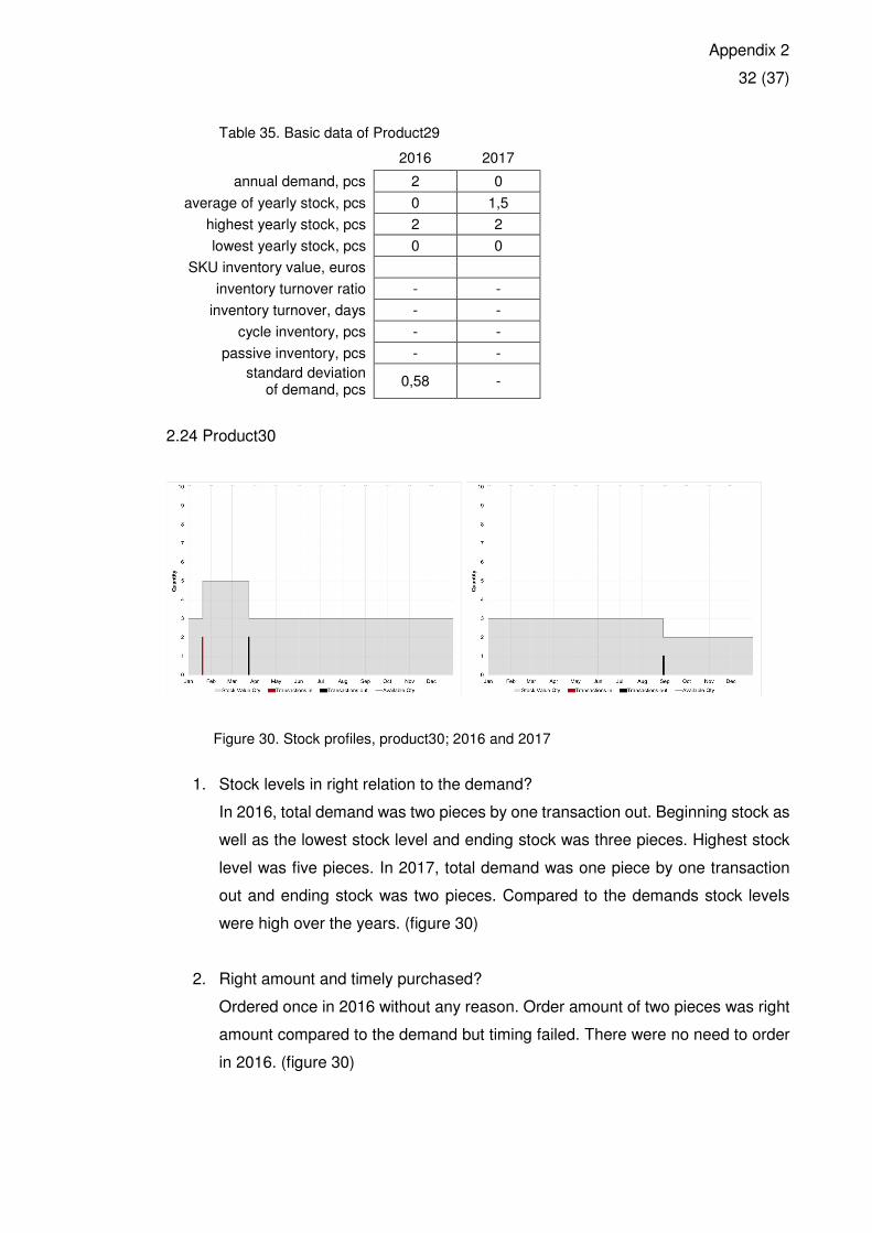
Appendix 2
32 (37)
Table 35. Basic data of Product29
2016 2017
annual demand, pcs 2 0
average of yearly stock, pcs 0 1,5
highest yearly stock, pcs 2 2
lowest yearly stock, pcs 0 0
SKU inventory value, euros
inventory turnover ratio - -
inventory turnover, days - -
cycle inventory, pcs - -
passive inventory, pcs - -
standard deviation of demand, pcs
0,58 -
2.24 Product30
Figure 30. Stock profiles, product30; 2016 and 2017
1. Stock levels in right relation to the demand?
In 2016, total demand was two pieces by one transaction out. Beginning stock as
well as the lowest stock level and ending stock was three pieces. Highest stock
level was five pieces. In 2017, total demand was one piece by one transaction
out and ending stock was two pieces. Compared to the demands stock levels
were high over the years. (figure 30)
2. Right amount and timely purchased?
Ordered once in 2016 without any reason. Order amount of two pieces was right
amount compared to the demand but timing failed. There were no need to order
in 2016. (figure 30)
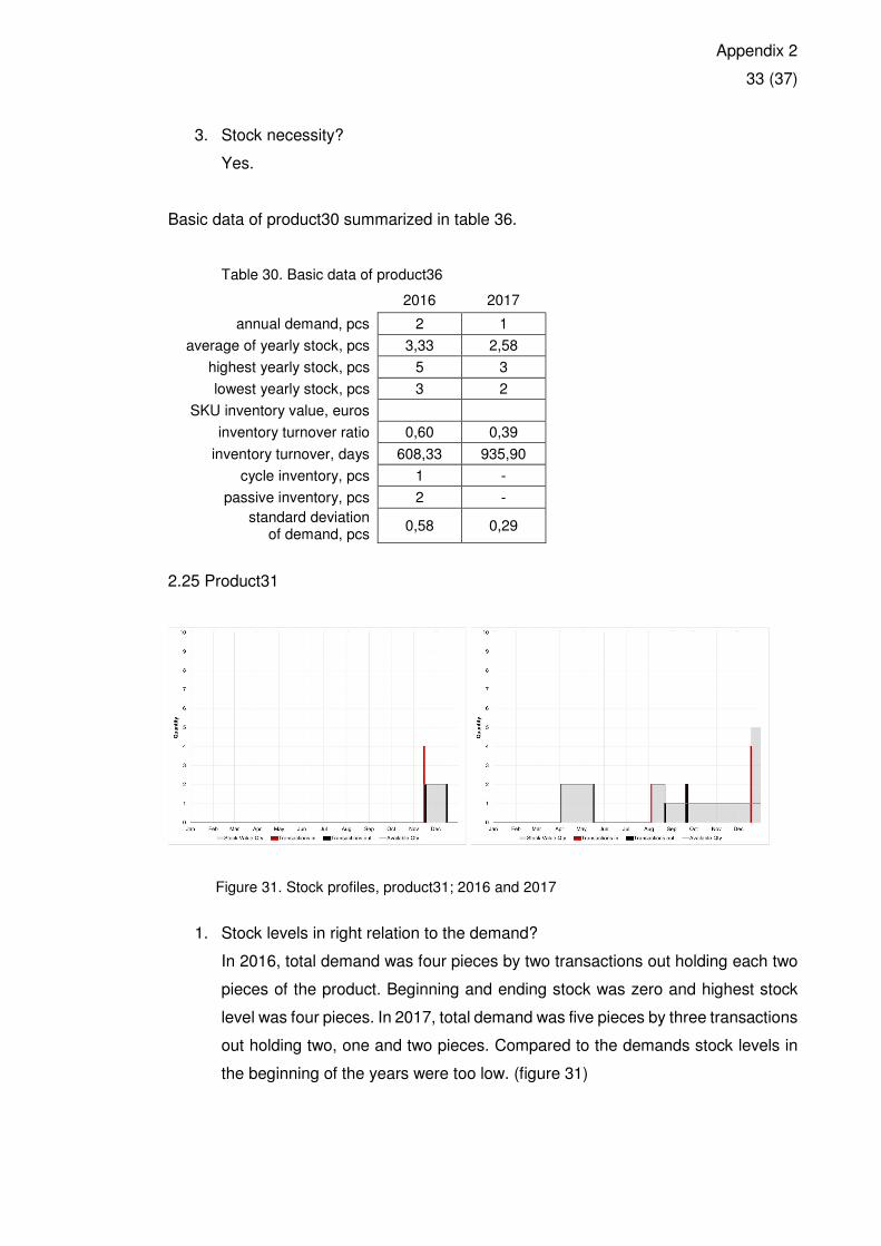
Appendix 2
33 (37)
3. Stock necessity?
Yes.
Basic data of product30 summarized in table 36.
Table 30. Basic data of product36
2016 2017
annual demand, pcs 2 1
average of yearly stock, pcs 3,33 2,58
highest yearly stock, pcs 5 3
lowest yearly stock, pcs 3 2
SKU inventory value, euros
inventory turnover ratio 0,60 0,39
inventory turnover, days 608,33 935,90
cycle inventory, pcs 1 -
passive inventory, pcs 2 -
standard deviation of demand, pcs
0,58 0,29
2.25 Product31
Figure 31. Stock profiles, product31; 2016 and 2017
1. Stock levels in right relation to the demand?
In 2016, total demand was four pieces by two transactions out holding each two
pieces of the product. Beginning and ending stock was zero and highest stock
level was four pieces. In 2017, total demand was five pieces by three transactions
out holding two, one and two pieces. Compared to the demands stock levels in
the beginning of the years were too low. (figure 31)
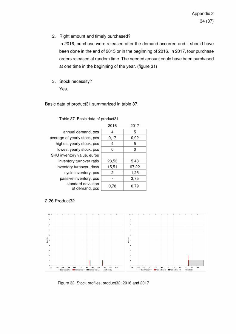
Appendix 2
34 (37)
2. Right amount and timely purchased?
In 2016, purchase were released after the demand occurred and it should have
been done in the end of 2015 or in the beginning of 2016. In 2017, four purchase
orders released at random time. The needed amount could have been purchased
at one time in the beginning of the year. (figure 31)
3. Stock necessity?
Yes.
Basic data of product31 summarized in table 37.
Table 37. Basic data of product31
2016 2017
annual demand, pcs 4 5
average of yearly stock, pcs 0,17 0,92
highest yearly stock, pcs 4 5
lowest yearly stock, pcs 0 0
SKU inventory value, euros
inventory turnover ratio 23,53 5,43
inventory turnover, days 15,51 67,22
cycle inventory, pcs 2 1,25
passive inventory, pcs - 3,75
standard deviation of demand, pcs
0,78 0,79
2.26 Product32
Figure 32. Stock profiles, product32; 2016 and 2017
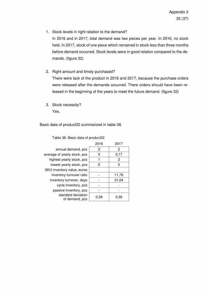
Appendix 2
35 (37)
1. Stock levels in right relation to the demand?
In 2016 and in 2017, total demand was two pieces per year. In 2016, no stock
held. In 2017, stock of one piece which remained in stock less than three months
before demand occurred. Stock levels were in good relation compared to the de-
mands. (figure 32)
2. Right amount and timely purchased?
There were lack of the product in 2016 and 2017, because the purchase orders
were released after the demands occurred. There orders should have been re-
leased in the beginning of the years to meet the future demand. (figure 32)
3. Stock necessity?
Yes.
Basic data of product32 summarized in table 38.
Table 38. Basic data of product32
2016 2017
annual demand, pcs 2 2
average of yearly stock, pcs 0 0,17
highest yearly stock, pcs 1 2
lowest yearly stock, pcs 0 0
SKU inventory value, euros
inventory turnover ratio - 11,76
inventory turnover, days - 31,04
cycle inventory, pcs - -
passive inventory, pcs - -
standard deviation of demand, pcs
0,39 0,39
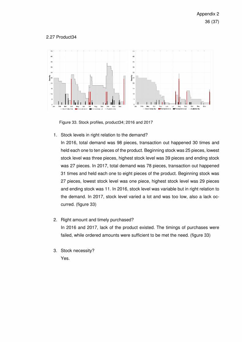
Appendix 2
36 (37)
2.27 Product34
Figure 33. Stock profiles, product34; 2016 and 2017
1. Stock levels in right relation to the demand?
In 2016, total demand was 98 pieces, transaction out happened 30 times and
held each one to ten pieces of the product. Beginning stock was 25 pieces, lowest
stock level was three pieces, highest stock level was 39 pieces and ending stock
was 27 pieces. In 2017, total demand was 78 pieces, transaction out happened
31 times and held each one to eight pieces of the product. Beginning stock was
27 pieces, lowest stock level was one piece, highest stock level was 29 pieces
and ending stock was 11. In 2016, stock level was variable but in right relation to
the demand. In 2017, stock level varied a lot and was too low, also a lack oc-
curred. (figure 33)
2. Right amount and timely purchased?
In 2016 and 2017, lack of the product existed. The timings of purchases were
failed, while ordered amounts were sufficient to be met the need. (figure 33)
3. Stock necessity?
Yes.
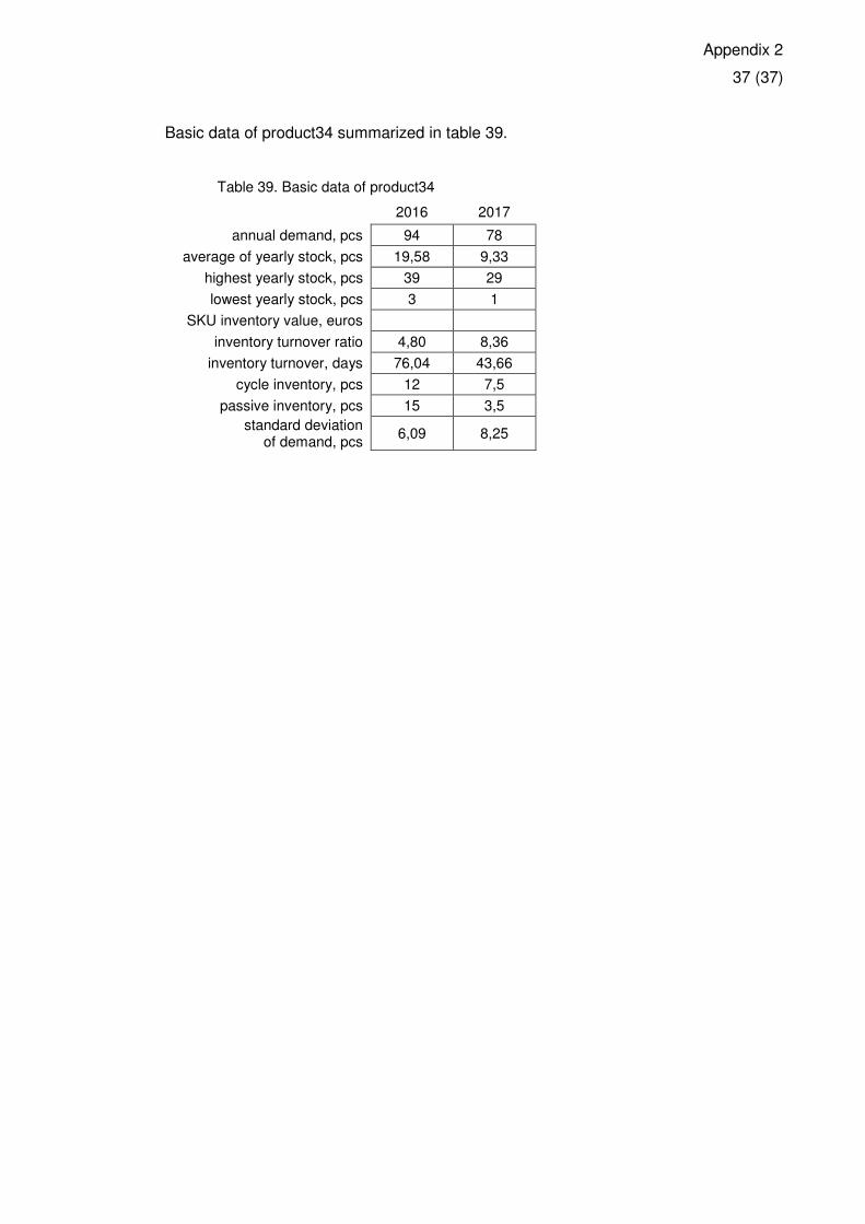
Appendix 2
37 (37)
Basic data of product34 summarized in table 39.
Table 39. Basic data of product34
2016 2017
annual demand, pcs 94 78
average of yearly stock, pcs 19,58 9,33
highest yearly stock, pcs 39 29
lowest yearly stock, pcs 3 1
SKU inventory value, euros
inventory turnover ratio 4,80 8,36
inventory turnover, days 76,04 43,66
cycle inventory, pcs 12 7,5
passive inventory, pcs 15 3,5
standard deviation of demand, pcs
6,09 8,25
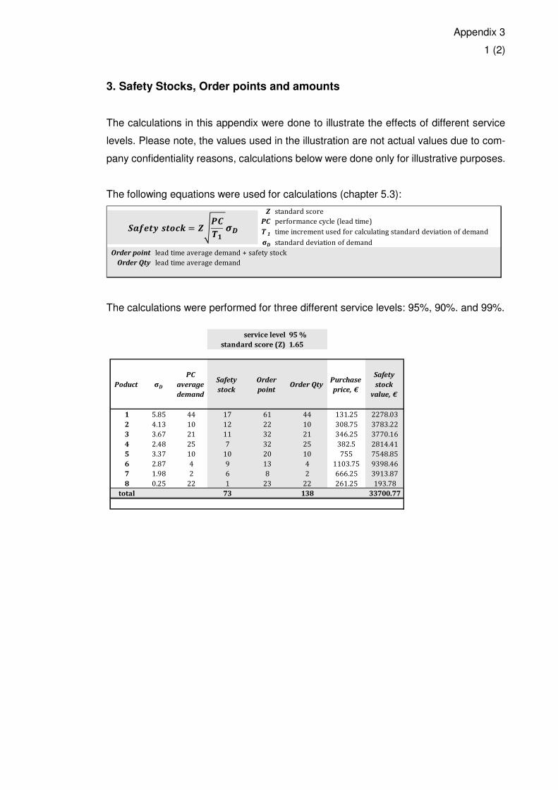
Appendix 3
1 (2)
3. Safety Stocks, Order points and amounts
The calculations in this appendix were done to illustrate the effects of different service
levels. Please note, the values used in the illustration are not actual values due to com-
pany confidentiality reasons, calculations below were done only for illustrative purposes.
The following equations were used for calculations (chapter 5.3):
The calculations were performed for three different service levels: 95%, 90%. and 99%.
Z standard score
PC performance cycle (lead time)
T 1 time increment used for calculating standard deviation of demand
σD standard deviation of demand
Order point lead time average demand + safety stock
Order Qty lead time average demand
\]^_`a b`cde = f ghij
kl\]^_`a b`cde = f ghij
kl
service level 95 %
standard score (Z) 1.65
Poduct σD
PC
average
demand
Safety
stock
Order
pointOrder Qty
Purchase
price, €
Safety
stock
value, €
1 5.85 44 17 61 44 131.25 2278.03
2 4.13 10 12 22 10 308.75 3783.22
3 3.67 21 11 32 21 346.25 3770.16
4 2.48 25 7 32 25 382.5 2814.41
5 3.37 10 10 20 10 755 7548.85
6 2.87 4 9 13 4 1103.75 9398.46
7 1.98 2 6 8 2 666.25 3913.87
8 0.25 22 1 23 22 261.25 193.78
total 73 138 33700.77
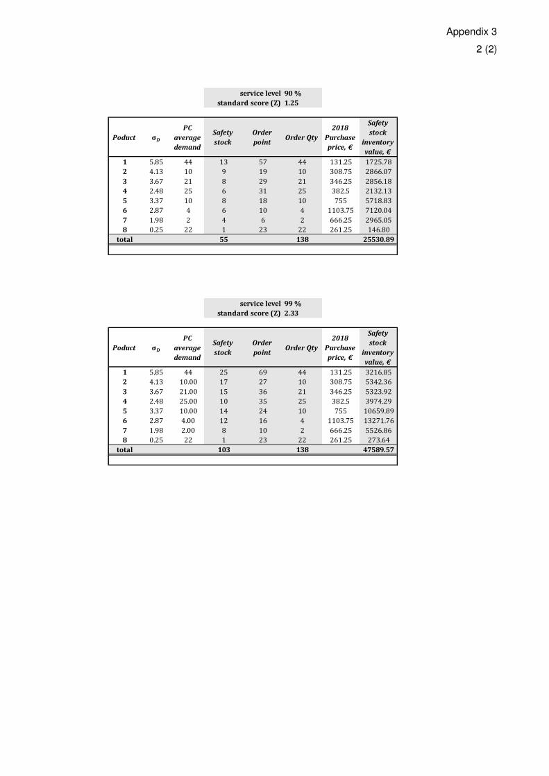
Appendix 3
2 (2)
service level 90 %
standard score (Z) 1.25
Poduct σD
PC
average
demand
Safety
stock
Order
pointOrder Qty
2018
Purchase
price, €
Safety
stock
inventory
value, €
1 5.85 44 13 57 44 131.25 1725.78
2 4.13 10 9 19 10 308.75 2866.07
3 3.67 21 8 29 21 346.25 2856.18
4 2.48 25 6 31 25 382.5 2132.13
5 3.37 10 8 18 10 755 5718.83
6 2.87 4 6 10 4 1103.75 7120.04
7 1.98 2 4 6 2 666.25 2965.05
8 0.25 22 1 23 22 261.25 146.80
total 55 138 25530.89
service level 99 %
standard score (Z) 2.33
Poduct σD
PC
average
demand
Safety
stock
Order
pointOrder Qty
2018
Purchase
price, €
Safety
stock
inventory
value, €
1 5.85 44 25 69 44 131.25 3216.85
2 4.13 10.00 17 27 10 308.75 5342.36
3 3.67 21.00 15 36 21 346.25 5323.92
4 2.48 25.00 10 35 25 382.5 3974.29
5 3.37 10.00 14 24 10 755 10659.89
6 2.87 4.00 12 16 4 1103.75 13271.76
7 1.98 2.00 8 10 2 666.25 5526.86
8 0.25 22 1 23 22 261.25 273.64
total 103 138 47589.57