Improving Lidar Turbulence Estimates for Wind Energy: … Lidar Turbulence Estimates for Wind Energy Preprint Jennifer Newman, Andrew Clifton, and Matthew Churchfield National Renewable

NREL is a national laboratory of the U.S. Department of Energy Office of Energy Efficiency & Renewable Energy Operated by the Alliance for Sustainable Energy, LLC

This report is available at no cost from the National Renewable Energy Laboratory (NREL) at www.nrel.gov/publications.

Contract No. DE-AC36-08GO28308

Improving Lidar Turbulence Estimates for Wind Energy Preprint Jennifer Newman, Andrew Clifton, and Matthew Churchfield National Renewable Energy Laboratory

Petra Klein University of Oklahoma

To be presented at the Science of Making Torque from Wind (TORQUE 2016) Munich, Germany October 5‒7, 2016

Conference Paper NREL/CP-5000-66994 October 2016

NOTICE

The submitted manuscript has been offered by an employee of the Alliance for Sustainable Energy, LLC (Alliance), a contractor of the US Government under Contract No. DE-AC36-08GO28308. Accordingly, the US Government and Alliance retain a nonexclusive royalty-free license to publish or reproduce the published form of this contribution, or allow others to do so, for US Government purposes.

This report was prepared as an account of work sponsored by an agency of the United States government. Neither the United States government nor any agency thereof, nor any of their employees, makes any warranty, express or implied, or assumes any legal liability or responsibility for the accuracy, completeness, or usefulness of any information, apparatus, product, or process disclosed, or represents that its use would not infringe privately owned rights. Reference herein to any specific commercial product, process, or service by trade name, trademark, manufacturer, or otherwise does not necessarily constitute or imply its endorsement, recommendation, or favoring by the United States government or any agency thereof. The views and opinions of authors expressed herein do not necessarily state or reflect those of the United States government or any agency thereof.


Available electronically at SciTech Connect http:/www.osti.gov/scitech

Available for a processing fee to U.S. Department of Energy and its contractors, in paper, from:

U.S. Department of Energy Office of Scientific and Technical Information P.O. Box 62 Oak Ridge, TN 37831-0062 OSTI http://www.osti.gov Phone: 865.576.8401 Fax: 865.576.5728 Email: [email protected]

Available for sale to the public, in paper, from:

U.S. Department of Commerce National Technical Information Service 5301 Shawnee Road Alexandria, VA 22312 NTIS http://www.ntis.gov Phone: 800.553.6847 or 703.605.6000 Fax: 703.605.6900 Email: [email protected]

Cover Photos by Dennis Schroeder: (left to right) NREL 26173, NREL 18302, NREL 19758, NREL 29642, NREL 19795.

NREL prints on paper that contains recycled content.

http://www.osti.gov/scitech

http://www.osti.gov/

mailto:[email protected]

http://www.ntis.gov/

mailto:[email protected]

Improving lidar turbulence estimates for wind energy

J F Newman1, A Clifton1, M J Churchfield1 and P Klein2

1 National Renewable Energy Laboratory, Golden, CO, USA2 School of Meteorology, University of Oklahoma, Norman, OK, USA

E-mail: [email protected]

Abstract. Remote sensing devices (e.g., lidars) are quickly becoming a cost-effective andreliable alternative to meteorological towers for wind energy applications. Although lidars canmeasure mean wind speeds accurately, these devices measure different values of turbulenceintensity (TI) than an instrument on a tower. In response to these issues, a lidar TI errorreduction model was recently developed for commercially available lidars. The TI error modelfirst applies physics-based corrections to the lidar measurements, then uses machine-learningtechniques to further reduce errors in lidar TI estimates. The model was tested at two sites inthe Southern Plains where vertically profiling lidars were collocated with meteorological towers.Results indicate that the model works well under stable conditions but cannot fully mitigatethe effects of variance contamination under unstable conditions. To understand how variancecontamination affects lidar TI estimates, a new set of equations was derived in previous work tocharacterize the actual variance measured by a lidar. Terms in these equations were quantifiedusing a lidar simulator and modeled wind field, and the new equations were then implementedinto the TI error model.

1. IntroductionProcedures such as wind resource assessment and turbine site suitability require measurementsof the mean wind speed and turbulence intensity (TI) at the turbine hub height. Traditionally,these measurements have been collected by cup anemometers on tall meteorological (met) towers.However, as modern turbine hub heights increase, it becomes more difficult and costly to installmet towers to reach hub height; in response, remote sensing devices (e.g., lidars, or light detectionand ranging devices) have recently emerged as alternatives to met towers. Although lidars haveseveral advantages over met towers, measurement methods used by lidars are fundamentallydifferent than those used by a cup or sonic anemometer. Anemometers provide an estimate ofthe wind speed at a small volume in space whereas lidars provide an average across a probevolume; this probe volume varies in length in the along-beam direction depending on the lidarused and is 20 m long for the WINDCUBE v2 lidar employed in this work. In addition, lidarsonly provide an estimate of the line-of-sight velocity and must point the lidar beam towarddifferent azimuth angles around a scanning circle to derive the full three-dimensional wind field.This scanning circle, which has a diameter of approximately 100 m for a commercial lidar ata measurement height of 100 m, introduces a phenomenon known as variance contamination[1]. Finally, instrument noise from the lidar can increase the variance estimated from the lidarmeasurements (for example, see [2]). All three of these factors—volume averaging, variancecontamination, and instrument noise—have negligible effects on the mean wind speed estimatedfrom the lidar but have profound effects on the lidar-estimated turbulence. Lidars must be


1

able to measure turbulence accurately to be viewed as a viable alternative to met towers in thewind energy industry. Thus, there is clearly a need for more accurate lidar-based turbulenceestimates, particularly for commercial lidars.

In response to this need for more accurate lidar turbulence estimates, an algorithmwas recently developed to reduce error in turbulence measurements from commercial lidars.The Lidar Turbulence Error Reduction Algorithm (L-TERRA) incorporates physics-basedcorrections, such as a spike filter and spectral corrections, in addition to machine-learningmethods to improve lidar turbulence estimates. In this paper, the development and testingof L-TERRA are discussed and results from two sites in the Southern Plains are shown. A lidarsimulator is used to improve the variance contamination corrections in L-TERRA and futureapplications of the lidar simulator in improving lidar turbulence estimates are discussed.

2. Background2.1. Lidar technologyLidars emit light waves into the atmosphere, which are then scattered by aerosol particles.A small portion of the scattered radiation returns to the lidar, and the Doppler shift of thereturned radiation is used to estimate the velocity in the line-of-sight of the lidar. In the caseof a pulsed Doppler lidar, the returned signal time series is split into blocks that correspond torange gates [3].

L-TERRA was initially developed for the WINDCUBE v2 lidar (Leosphere, Orsay, France),hereafter referred to as “WC,” a commercially available, pulsed Doppler lidar that is commonlyused in the wind energy industry. The WC uses a Doppler-beam swinging (DBS) [4] technique toestimate the three-dimensional wind profile, wherein the lidar beam is pointed in the north, east,south, and west directions and geometrical relations are used to estimate the u, v, and w windcomponents. The WINDCUBE v2 model, which was used in this work, includes a verticallypointing beam position to obtain a direct measurement of the vertical velocity. The WCaccumulates measurements at each scanning location for 1 s, and a full scan takes approximately4 s. However, the device’s software updates the velocity vector every time the beam moves to anew location, such that the output data stream of velocity is available at 1 Hz.

2.2. Sources of lidar turbulence errorThree primary factors impact the accuracy of lidar turbulence estimates: instrument noise,volume averaging, and variance contamination. The first two factors are inherent to remotesensing technology and impact any type of lidar regardless of the scanning technique used.Instrument noise results from factors such as the limited amount of scatterers in the lidar probevolume (for example, see [2]) and spontaneous laser emissions [5]. Volume averaging occursbecause the lidar must receive backscattered radiation from a volume of air, rather than a point,to obtain a sufficient amount of data for estimation of the radial wind speed. For the WC lidarused in this work, the sample volume is 20 m in length and negligibly small in the cross-beamdirection [6]. Thus, the lidar-measured wind speed at a height of 100 m is actually a weightedaverage of all the aerosol particle velocities between 90 and 110 m. The probe volume acts asa low-pass filter, as high-frequency motion that occurs on spatial scales smaller than the probevolume of the lidar cannot be resolved.

The third factor, variance contamination, is caused by the scanning strategy used by the lidar.When velocity data from different parts of the lidar scanning circle are combined to estimate theraw wind speed components, it is assumed that the instantaneous wind field is uniform acrossthe scanning circle. However, this assumption is not true in turbulent flow, and changes in thewind field across the lidar scanning circle introduce additional variance components into thecalculation of the u, v, and w variance (for example, see [1] and [7]).


2

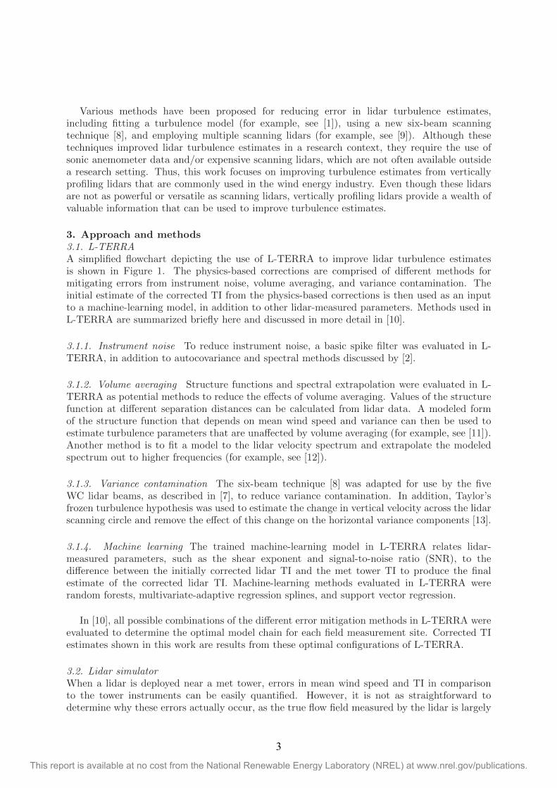
Various methods have been proposed for reducing error in lidar turbulence estimates,including fitting a turbulence model (for example, see [1]), using a new six-beam scanningtechnique [8], and employing multiple scanning lidars (for example, see [9]). Although thesetechniques improved lidar turbulence estimates in a research context, they require the use ofsonic anemometer data and/or expensive scanning lidars, which are not often available outsidea research setting. Thus, this work focuses on improving turbulence estimates from verticallyprofiling lidars that are commonly used in the wind energy industry. Even though these lidarsare not as powerful or versatile as scanning lidars, vertically profiling lidars provide a wealth ofvaluable information that can be used to improve turbulence estimates.

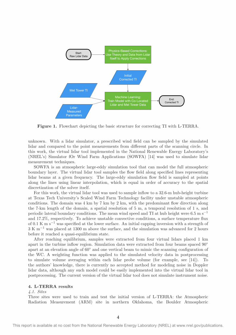
3. Approach and methods3.1. L-TERRAA simplified flowchart depicting the use of L-TERRA to improve lidar turbulence estimatesis shown in Figure 1. The physics-based corrections are comprised of different methods formitigating errors from instrument noise, volume averaging, and variance contamination. Theinitial estimate of the corrected TI from the physics-based corrections is then used as an inputto a machine-learning model, in addition to other lidar-measured parameters. Methods used inL-TERRA are summarized briefly here and discussed in more detail in [10].

3.1.1. Instrument noise To reduce instrument noise, a basic spike filter was evaluated in L-TERRA, in addition to autocovariance and spectral methods discussed by [2].

3.1.2. Volume averaging Structure functions and spectral extrapolation were evaluated in L-TERRA as potential methods to reduce the effects of volume averaging. Values of the structurefunction at different separation distances can be calculated from lidar data. A modeled formof the structure function that depends on mean wind speed and variance can then be used toestimate turbulence parameters that are unaffected by volume averaging (for example, see [11]).Another method is to fit a model to the lidar velocity spectrum and extrapolate the modeledspectrum out to higher frequencies (for example, see [12]).

3.1.3. Variance contamination The six-beam technique [8] was adapted for use by the fiveWC lidar beams, as described in [7], to reduce variance contamination. In addition, Taylor’sfrozen turbulence hypothesis was used to estimate the change in vertical velocity across the lidarscanning circle and remove the effect of this change on the horizontal variance components [13].

3.1.4. Machine learning The trained machine-learning model in L-TERRA relates lidar-measured parameters, such as the shear exponent and signal-to-noise ratio (SNR), to thedifference between the initially corrected lidar TI and the met tower TI to produce the finalestimate of the corrected lidar TI. Machine-learning methods evaluated in L-TERRA wererandom forests, multivariate-adaptive regression splines, and support vector regression.

In [10], all possible combinations of the different error mitigation methods in L-TERRA wereevaluated to determine the optimal model chain for each field measurement site. Corrected TIestimates shown in this work are results from these optimal configurations of L-TERRA.

3.2. Lidar simulatorWhen a lidar is deployed near a met tower, errors in mean wind speed and TI in comparisonto the tower instruments can be easily quantified. However, it is not as straightforward todetermine why these errors actually occur, as the true flow field measured by the lidar is largely


3

Physics-Based Corrections:

Use Theory and Data from Lidar

Itself to Apply Corrections

Start:

Raw Lidar Data

Initial

Corrected TI

End:

Corrected TI

Machine Learning:

Train Model with Co-Located

Lidar and Met Tower Data

Met Tower TI

Lidar-

Measured

Parameters

Figure 1. Flowchart depicting the basic structure for correcting TI with L-TERRA.

unknown. With a lidar simulator, a prescribed wind field can be sampled by the simulatedlidar and compared to the point measurements from different parts of the scanning circle. Inthis work, the virtual lidar tool implemented in the National Renewable Energy Laboratory’s(NREL’s) Simulator fOr Wind Farm Applications (SOWFA) [14] was used to simulate lidarmeasurement techniques.

SOWFA is an atmospheric large-eddy simulation tool that can model the full atmosphericboundary layer. The virtual lidar tool samples the flow field along specified lines representinglidar beams at a given frequency. The large-eddy simulation flow field is sampled at pointsalong the lines using linear interpolation, which is equal in order of accuracy to the spatialdiscretization of the solver itself.

For this work, the virtual lidar tool was used to sample inflow to a 32.6-m hub-height turbineat Texas Tech University’s Scaled Wind Farm Technology facility under unstable atmosphericconditions. The domain was 4 km by 7 km by 2 km, with the predominant flow direction alongthe 7-km length of the domain, a spatial resolution of 5 m, a temporal resolution of 1 s, andperiodic lateral boundary conditions. The mean wind speed and TI at hub height were 6.5 m s−1

and 17.2%, respectively. To achieve unstable convective conditions, a surface temperature fluxof 0.1 K m s−1 was specified at the lower surface. An initial capping inversion with a strength of3 K m−1 was placed at 1300 m above the surface, and the simulation was advanced for 2 hoursbefore it reached a quasi-equilibrium state.

After reaching equilibrium, samples were extracted from four virtual lidars placed 1 kmapart in the turbine inflow region. Simulation data were extracted from four beams spaced 90◦

apart at an elevation angle of 60◦ and one vertical beam to mimic the scanning configuration ofthe WC. A weighting function was applied to the simulated velocity data in postprocessingto simulate volume averaging within each lidar probe volume (for example, see [14]). Tothe authors’ knowledge, there is currently no accepted method for modeling noise in Dopplerlidar data, although any such model could be easily implemented into the virtual lidar tool inpostprocessing. The current version of the virtual lidar tool does not simulate instrument noise.

4. L-TERRA results4.1. SitesThree sites were used to train and test the initial version of L-TERRA: the AtmosphericRadiation Measurement (ARM) site in northern Oklahoma, the Boulder Atmospheric


4

Observatory (BAO) in Erie, Colorado, and an operational wind farm in the Southern GreatPlains region of the United States. Because of a nondisclosure agreement with the wind farm,its exact location cannot be disclosed. Only data from the ARM site and wind farm are shownin this work, as lidar data availability was low at the BAO due to a low aerosol count.

The ARM site is a field measurement site operated by the U.S. Department of Energy thatcontains a variety of in-situ and remote sensing instruments [15]. From November 2012 to July2013, a WC lidar was deployed 100 m northeast of a 60-m tower at the ARM site with GillWindmaster Pro 3-D sonic anemometers mounted at 25 and 60 m above ground level (AGL).The WC was then deployed at the operational wind farm from November 2013 to January 2014and again from May to July 2014. While at the wind farm, the WC was located in the sameenclosure as a met tower containing standard wind energy instrumentation. The tower had alattice structure and the WC was positioned such that none of the beam positions were blockedby the tower. The closest turbine was approximately 240 m from the tower enclosure, and onlymeasurements from nonwaked wind directions were used in this work.

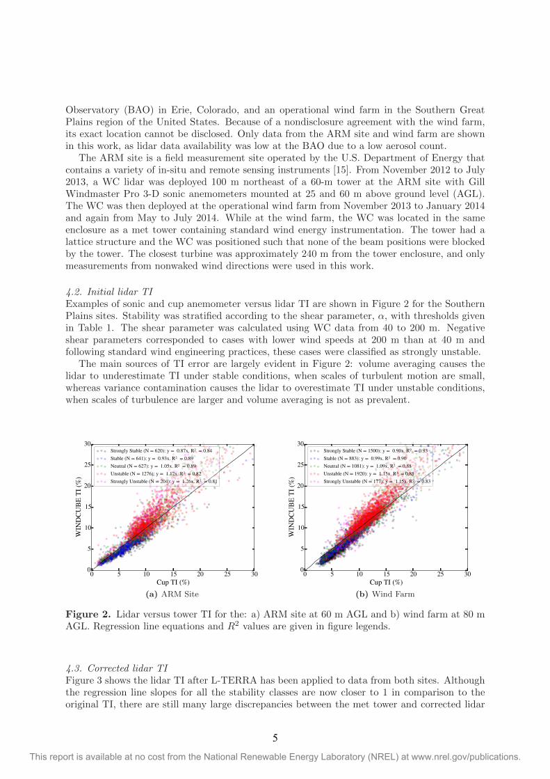
4.2. Initial lidar TIExamples of sonic and cup anemometer versus lidar TI are shown in Figure 2 for the SouthernPlains sites. Stability was stratified according to the shear parameter, α, with thresholds givenin Table 1. The shear parameter was calculated using WC data from 40 to 200 m. Negativeshear parameters corresponded to cases with lower wind speeds at 200 m than at 40 m andfollowing standard wind engineering practices, these cases were classified as strongly unstable.

The main sources of TI error are largely evident in Figure 2: volume averaging causes thelidar to underestimate TI under stable conditions, when scales of turbulent motion are small,whereas variance contamination causes the lidar to overestimate TI under unstable conditions,when scales of turbulence are larger and volume averaging is not as prevalent.

0 5 10 15 20 25 30Cup TI (%)

0

5

10

15

20

25

30

WIN

DCUB

E TI

(%)

Strongly Stable (N = 620): y = 0.87x. R2 = 0.84Stable (N = 641): y = 0.93x. R2 = 0.89Neutral (N = 627): y = 1.05x. R2 = 0.89Unstable (N = 1276): y = 1.12x. R2 = 0.82Strongly Unstable (N = 204): y = 1.26x. R2 = 0.81

(a) ARM Site

0 5 10 15 20 25 30Cup TI (%)

0

5

10

15

20

25

30

WIN

DCUB

E TI

(%)


(b) Wind Farm

Figure 2. Lidar versus tower TI for the: a) ARM site at 60 m AGL and b) wind farm at 80 mAGL. Regression line equations and R2 values are given in figure legends.

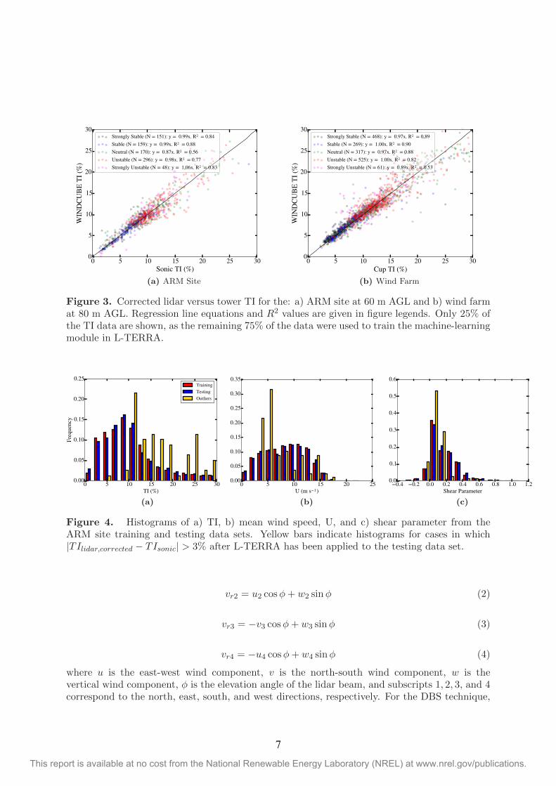
4.3. Corrected lidar TIFigure 3 shows the lidar TI after L-TERRA has been applied to data from both sites. Althoughthe regression line slopes for all the stability classes are now closer to 1 in comparison to theoriginal TI, there are still many large discrepancies between the met tower and corrected lidar


5

Table 1. Stability classifications used in this work.

Stability Classification Shear Parameter RangeStrongly stable α ≥ 0.3

Stable 0.2 ≤ α < 0.3Neutral 0.1 ≤ α < 0.2

Unstable 0 ≤ α < 0.1Strongly unstable α < 0

TI. To identify conditions under which L-TERRA performance is suboptimal, histograms of TI,mean wind speed, and the shear parameter were examined for periods in which the differencebetween the corrected lidar TI and met tower TI was still greater than 3%. At the ARM site,these periods comprised 5.2% of the testing data set. Before L-TERRA was applied, 12.2% ofthe lidar TI values in the testing data set had an error of more than 3%.

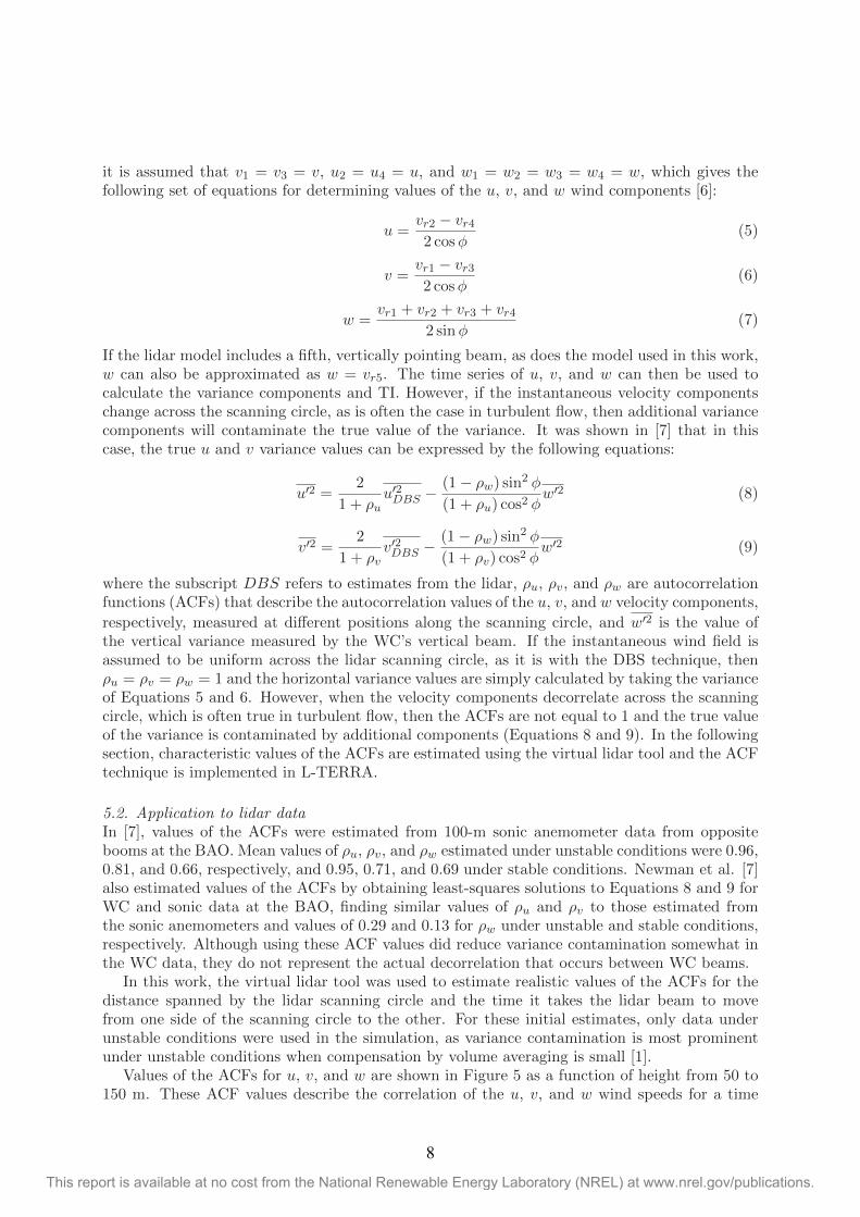
Histograms from the ARM site are shown in Figure 4. Large differences between the correctedlidar TI and sonic TI tend to occur when the lidar measures high TI values, low mean wind speedvalues, and low shear parameter values in comparison to the testing data set as a whole. Thesetrends typically correspond to unstable atmospheric conditions, suggesting that in their currentform, neither the physics-based corrections nor the machine-learning techniques in L-TERRAcan adequately mitigate the effects of variance contamination. The initial version of the variancecontamination module utilizes Taylor’s frozen turbulence hypothesis, which is less valid forlower wind speeds when turbulent eddies are more likely to evolve as they move across thelidar scanning circle. Thus, it is not surprising that large TI errors remain for low wind speedconditions.

It is also likely that the machine-learning portion of L-TERRA did not have an adequateamount of training data under these high-TI, low wind speed conditions. The histogramsshown in Figure 4 indicate that outlier conditions correspond to the tail of the TI trainingset distribution and the far left ends of the mean wind speed and shear distributions. Thus,the conditions under which L-TERRA performed most poorly also correspond to conditions inwhich the machine-learning model was not supplied with a large amount of training data andis not expected to perform as well. This highlights the need for a large training data set forL-TERRA that includes a wide range of conditions.

5. New method for reducing variance contamination5.1. Theoretical backgroundA series of equations was developed in [7] to relate the variance measured by a lidar with aDBS technique to the true value of the variance through the use of autocorrelation functions(ACFs). This series of equations is essentially a simplified version of the results presented in [1],in which a model of the spectral velocity tensor is convolved with a volume-averaging functionto estimate the variance that would be measured by a lidar. This modeling approach typicallyrequires fitting parameters to sonic anemometer data and is technically only valid under neutralconditions. In contrast, the technique presented in this work does not require the fitting of amodel and is much simpler to implement. A brief overview of the development of this techniqueis given here.

The radial velocity, vr, measured with the DBS technique at different beam positions, can bedescribed by the following equations:

vr1 = v1 cosφ+ w1 sinφ (1)


6

0 5 10 15 20 25 30Sonic TI (%)

0

5

10

15

20

25

30

WIN

DCUB

E TI

(%)


(a) ARM Site

0 5 10 15 20 25 30Cup TI (%)

0

5

10

15

20

25

30

WIN

DCUB

E TI

(%)


(b) Wind Farm

Figure 3. Corrected lidar versus tower TI for the: a) ARM site at 60 m AGL and b) wind farmat 80 m AGL. Regression line equations and R2 values are given in figure legends. Only 25% ofthe TI data are shown, as the remaining 75% of the data were used to train the machine-learningmodule in L-TERRA.

0 5 10 15 20 25 30TI (%)

0.00

0.05

0.10

0.15

0.20

0.25

Freq

uenc

y

TrainingTestingOutliers

(a)

0 5 10 15 20 25U (m s 1)

0.00

0.05

0.10

0.15

0.20

0.25

0.30

0.35

(b)

0.4 0.2 0.0 0.2 0.4 0.6 0.8 1.0 1.2Shear Parameter

0.0

0.1

0.2

0.3

0.4

0.5

0.6

(c)

Figure 4. Histograms of a) TI, b) mean wind speed, U, and c) shear parameter from theARM site training and testing data sets. Yellow bars indicate histograms for cases in which|TIlidar,corrected − TIsonic| > 3% after L-TERRA has been applied to the testing data set.

vr2 = u2 cosφ+ w2 sinφ (2)

vr3 = −v3 cosφ+ w3 sinφ (3)

vr4 = −u4 cosφ+ w4 sinφ (4)

where u is the east-west wind component, v is the north-south wind component, w is thevertical wind component, φ is the elevation angle of the lidar beam, and subscripts 1, 2, 3, and 4correspond to the north, east, south, and west directions, respectively. For the DBS technique,


7

it is assumed that v1 = v3 = v, u2 = u4 = u, and w1 = w2 = w3 = w4 = w, which gives thefollowing set of equations for determining values of the u, v, and w wind components [6]:

u =vr2 − vr42 cosφ

(5)

v =vr1 − vr32 cosφ

(6)

w =vr1 + vr2 + vr3 + vr4

2 sinφ(7)

If the lidar model includes a fifth, vertically pointing beam, as does the model used in this work,w can also be approximated as w = vr5. The time series of u, v, and w can then be used tocalculate the variance components and TI. However, if the instantaneous velocity componentschange across the scanning circle, as is often the case in turbulent flow, then additional variancecomponents will contaminate the true value of the variance. It was shown in [7] that in thiscase, the true u and v variance values can be expressed by the following equations:

u′2 =2

1 + ρuu′2DBS −

(1− ρw) sin2 φ

(1 + ρu) cos2 φw′2 (8)

v′2 =2

1 + ρvv′2DBS −

(1− ρw) sin2 φ

(1 + ρv) cos2 φw′2 (9)

where the subscript DBS refers to estimates from the lidar, ρu, ρv, and ρw are autocorrelationfunctions (ACFs) that describe the autocorrelation values of the u, v, and w velocity components,

respectively, measured at different positions along the scanning circle, and w′2 is the value ofthe vertical variance measured by the WC’s vertical beam. If the instantaneous wind field isassumed to be uniform across the lidar scanning circle, as it is with the DBS technique, thenρu = ρv = ρw = 1 and the horizontal variance values are simply calculated by taking the varianceof Equations 5 and 6. However, when the velocity components decorrelate across the scanningcircle, which is often true in turbulent flow, then the ACFs are not equal to 1 and the true valueof the variance is contaminated by additional components (Equations 8 and 9). In the followingsection, characteristic values of the ACFs are estimated using the virtual lidar tool and the ACFtechnique is implemented in L-TERRA.

5.2. Application to lidar dataIn [7], values of the ACFs were estimated from 100-m sonic anemometer data from oppositebooms at the BAO. Mean values of ρu, ρv, and ρw estimated under unstable conditions were 0.96,0.81, and 0.66, respectively, and 0.95, 0.71, and 0.69 under stable conditions. Newman et al. [7]also estimated values of the ACFs by obtaining least-squares solutions to Equations 8 and 9 forWC and sonic data at the BAO, finding similar values of ρu and ρv to those estimated fromthe sonic anemometers and values of 0.29 and 0.13 for ρw under unstable and stable conditions,respectively. Although using these ACF values did reduce variance contamination somewhat inthe WC data, they do not represent the actual decorrelation that occurs between WC beams.

In this work, the virtual lidar tool was used to estimate realistic values of the ACFs for thedistance spanned by the lidar scanning circle and the time it takes the lidar beam to movefrom one side of the scanning circle to the other. For these initial estimates, only data underunstable conditions were used in the simulation, as variance contamination is most prominentunder unstable conditions when compensation by volume averaging is small [1].

Values of the ACFs for u, v, and w are shown in Figure 5 as a function of height from 50 to150 m. These ACF values describe the correlation of the u, v, and w wind speeds for a time


8

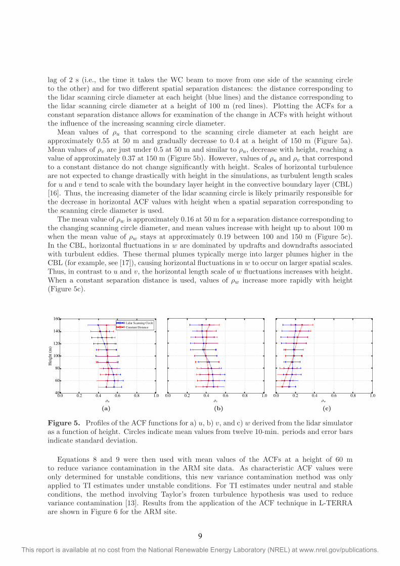
lag of 2 s (i.e., the time it takes the WC beam to move from one side of the scanning circleto the other) and for two different spatial separation distances: the distance corresponding tothe lidar scanning circle diameter at each height (blue lines) and the distance corresponding tothe lidar scanning circle diameter at a height of 100 m (red lines). Plotting the ACFs for aconstant separation distance allows for examination of the change in ACFs with height withoutthe influence of the increasing scanning circle diameter.

Mean values of ρu that correspond to the scanning circle diameter at each height areapproximately 0.55 at 50 m and gradually decrease to 0.4 at a height of 150 m (Figure 5a).Mean values of ρv are just under 0.5 at 50 m and similar to ρu, decrease with height, reaching avalue of approximately 0.37 at 150 m (Figure 5b). However, values of ρu and ρv that correspondto a constant distance do not change significantly with height. Scales of horizontal turbulenceare not expected to change drastically with height in the simulations, as turbulent length scalesfor u and v tend to scale with the boundary layer height in the convective boundary layer (CBL)[16]. Thus, the increasing diameter of the lidar scanning circle is likely primarily responsible forthe decrease in horizontal ACF values with height when a spatial separation corresponding tothe scanning circle diameter is used.

The mean value of ρw is approximately 0.16 at 50 m for a separation distance corresponding tothe changing scanning circle diameter, and mean values increase with height up to about 100 mwhen the mean value of ρw stays at approximately 0.19 between 100 and 150 m (Figure 5c).In the CBL, horizontal fluctuations in w are dominated by updrafts and downdrafts associatedwith turbulent eddies. These thermal plumes typically merge into larger plumes higher in theCBL (for example, see [17]), causing horizontal fluctuations in w to occur on larger spatial scales.Thus, in contrast to u and v, the horizontal length scale of w fluctuations increases with height.When a constant separation distance is used, values of ρw increase more rapidly with height(Figure 5c).

0.0 0.2 0.4 0.6 0.8 1.0u

40

60

80

100

120

140

160

Heig

ht (m

)

Lidar Scanning CircleConstant Distance

(a)

0.0 0.2 0.4 0.6 0.8 1.0v

(b)

0.0 0.2 0.4 0.6 0.8 1.0w

(c)

Figure 5. Profiles of the ACF functions for a) u, b) v, and c) w derived from the lidar simulatoras a function of height. Circles indicate mean values from twelve 10-min. periods and error barsindicate standard deviation.

Equations 8 and 9 were then used with mean values of the ACFs at a height of 60 mto reduce variance contamination in the ARM site data. As characteristic ACF values wereonly determined for unstable conditions, this new variance contamination method was onlyapplied to TI estimates under unstable conditions. For TI estimates under neutral and stableconditions, the method involving Taylor’s frozen turbulence hypothesis was used to reducevariance contamination [13]. Results from the application of the ACF technique in L-TERRAare shown in Figure 6 for the ARM site.


9

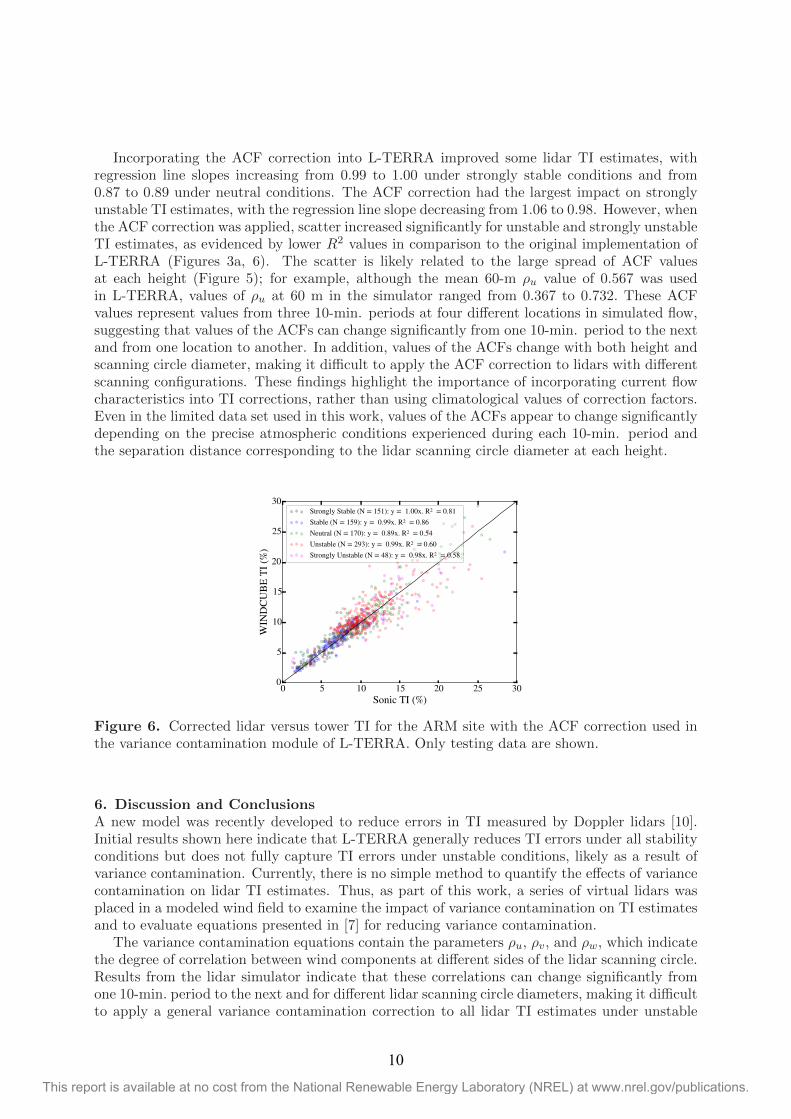
Incorporating the ACF correction into L-TERRA improved some lidar TI estimates, withregression line slopes increasing from 0.99 to 1.00 under strongly stable conditions and from0.87 to 0.89 under neutral conditions. The ACF correction had the largest impact on stronglyunstable TI estimates, with the regression line slope decreasing from 1.06 to 0.98. However, whenthe ACF correction was applied, scatter increased significantly for unstable and strongly unstableTI estimates, as evidenced by lower R2 values in comparison to the original implementation ofL-TERRA (Figures 3a, 6). The scatter is likely related to the large spread of ACF valuesat each height (Figure 5); for example, although the mean 60-m ρu value of 0.567 was usedin L-TERRA, values of ρu at 60 m in the simulator ranged from 0.367 to 0.732. These ACFvalues represent values from three 10-min. periods at four different locations in simulated flow,suggesting that values of the ACFs can change significantly from one 10-min. period to the nextand from one location to another. In addition, values of the ACFs change with both height andscanning circle diameter, making it difficult to apply the ACF correction to lidars with differentscanning configurations. These findings highlight the importance of incorporating current flowcharacteristics into TI corrections, rather than using climatological values of correction factors.Even in the limited data set used in this work, values of the ACFs appear to change significantlydepending on the precise atmospheric conditions experienced during each 10-min. period andthe separation distance corresponding to the lidar scanning circle diameter at each height.

0 5 10 15 20 25 30Sonic TI (%)

0

5

10

15

20

25

30

WIN

DCUB

E TI

(%)


Figure 6. Corrected lidar versus tower TI for the ARM site with the ACF correction used inthe variance contamination module of L-TERRA. Only testing data are shown.

6. Discussion and ConclusionsA new model was recently developed to reduce errors in TI measured by Doppler lidars [10].Initial results shown here indicate that L-TERRA generally reduces TI errors under all stabilityconditions but does not fully capture TI errors under unstable conditions, likely as a result ofvariance contamination. Currently, there is no simple method to quantify the effects of variancecontamination on lidar TI estimates. Thus, as part of this work, a series of virtual lidars wasplaced in a modeled wind field to examine the impact of variance contamination on TI estimatesand to evaluate equations presented in [7] for reducing variance contamination.

The variance contamination equations contain the parameters ρu, ρv, and ρw, which indicatethe degree of correlation between wind components at different sides of the lidar scanning circle.Results from the lidar simulator indicate that these correlations can change significantly fromone 10-min. period to the next and for different lidar scanning circle diameters, making it difficultto apply a general variance contamination correction to all lidar TI estimates under unstable


10

conditions. When mean values of the ACFs were used to reduce variance contamination inL-TERRA, some lidar TI estimates improved, but scatter increased. This result suggests thatthe variance contamination method must adapt to the differing atmospheric conditions duringeach 10-min. time period to accurately reduce variance contamination. Future work will involveusing available lidar data to quantify the degree of variance contamination during each 10-min. period. By using data from the lidar itself, rather than a generalized equation, variancecontamination can be quantified more accurately for different sites and under different kinds ofstability conditions. Variance contamination corrections can be tested with the virtual lidar toolto examine the validity of the corrections for different lidar scanning geometries, measurementheights, and atmospheric conditions.

AcknowledgmentsThe authors would like to thank the scientists and staff members who assisted with the ARMsite, BAO, and wind farm deployments. Sebastien Biraud and Marc Fischer supplied sonicanemometer data for the ARM site, and Andreas Muschinski provided sonic anemometer data forthe BAO. Sonia Wharton of Lawrence Livermore National Laboratory provided the WINDCUBElidar used in this work and assisted with field deployments. The ARM Climate Research Facilityis a U.S. Department of Energy Office of Science user facility sponsored by the Office of Biologicaland Environmental Research. This work was supported by the U.S. Department of Energy underContract No. DE-AC36-08GO28308 with the National Renewable Energy Laboratory. Fundingfor the work was provided by the DOE Office of Energy Efficiency and Renewable Energy,Wind and Water Power Technologies Office. The U.S. Government retains and the publisher,by accepting the article for publication, acknowledges that the U.S. Government retains anonexclusive, paid-up, irrevocable, worldwide license to publish or reproduce the published formof this work, or allow others to do so, for U.S. Government purposes.

References[1] Sathe A, Mann J, Gottschall J and Courtney M S 2011 J. Atmos. Oceanic Technol. 28

853–868

[2] Lenschow D H, Wulfmeyer V and Senff C 2000 J. Atmos. Oceanic Technol. 17 1330–1347

[3] Huffaker R M and Hardesty R M 1996 Proceedings of the IEEE 84 181–204

[4] Strauch R G, Merritt D A, Moran K P, Earnshaw K B and De Kamp D V 1984 J. Atmos.Oceanic Technol. 1 37–49

[5] Chang W S 2005 Principles of Lasers and Optics (Cambridge University Press)

[6] Pena A et al. 2015 Remote sensing for wind energy Tech. Rep. DTU Wind Energy-E-Report-008 Denmark Technical University

[7] Newman J F, Klein P M, Wharton S, Sathe A, Bonin T A, Chilson P B and Muschinski A2016 Atmos. Meas. Tech. 9 1993–2013

[8] Sathe A, Mann J, Vasiljevic N and Lea G 2015 Atmos. Meas. Tech. 8 729–740

[9] Fuertes F C, Iungo G V and Porte-Agel F 2014 J. Atmos. Oceanic Technol. 31 1549–1556

[10] Newman J F and Clifton A 2016 Wind Energ. Sci. Discuss. In review, doi:10.5194/wes–2016–22

[11] Krishnamurthy R, Calhoun R, Billings B and Doyle J 2011 Meteorological Applications 18361–371

[12] Hogan R J, Grant A L, Illingworth A J, Pearson G N and O’Connor E J 2009 Quart. J.Roy. Meteor. Soc. 135 635–643

[13] Newman J F 2015 Optimizing lidar scanning strategies for wind energy turbulencemeasurements Ph.D. thesis University of Oklahoma Norman, Oklahoma, USA


11

[14] Lundquist J K, Churchfield M J, Lee S and Clifton A 2015 Atmos. Meas. Tech. 8 907–920

[15] Mather J H and Voyles J W 2013 Bull. Amer. Meteor. Soc. 94 377–392

[16] Kaimal J C, Wyngaard J C, Haugen D A, Cote O R, Izumi Y, Caughey S J and ReadingsC J 1976 J. Atmos. Sci. 33 2152–2169

[17] Garratt J 1992 The Atmospheric Boundary Layer (Cambridge University Press)


12

Documents

Improving Lidar Turbulence Estimates for Wind Energy: … Lidar Turbulence Estimates for Wind Energy Preprint Jennifer Newman, Andrew Clifton, and Matthew Churchfield National Renewable