Embed Size (px)
Citation preview
HAL Id: tel-01661536https://tel.archives-ouvertes.fr/tel-01661536
Submitted on 12 Dec 2017
HAL is a multi-disciplinary open accessarchive for the deposit and dissemination of sci-entific research documents, whether they are pub-lished or not. The documents may come fromteaching and research institutions in France orabroad, or from public or private research centers.
L’archive ouverte pluridisciplinaire HAL, estdestinée au dépôt et à la diffusion de documentsscientifiques de niveau recherche, publiés ou non,émanant des établissements d’enseignement et derecherche français ou étrangers, des laboratoirespublics ou privés.
Improvement of the numerical capacities of simulationtools for reactive transport modeling in porous media
Daniel Jara Heredia
To cite this version:Daniel Jara Heredia. Improvement of the numerical capacities of simulation tools for reactive trans-port modeling in porous media. Earth Sciences. Université Rennes 1, 2017. English. �NNT :2017REN1S036�. �tel-01661536�
ANNÉE 2017
THÈSE / UNIVERSITÉ DE RENNES 1 sous le sceau de l’Université Bretagne Loire
pour le grade de
DOCTEUR DE L’UNIVERSITÉ DE RENNES 1 Mention : Sciences de la Terre
Ecole doctorale Sciences de la Matière
Daniel JARA HEREDIA Préparée à l’unité de recherche Géosciences Rennes
(UMR CNRS 6118) OSUR Observatoire des Sciences de l'Univers de Rennes
Improvement of the numerical capacities of simulation tools for reactive transport modeling in porous media.
Thèse soutenue à Rennes le 21 Juin 2017 :
devant le jury composé de :
Michel KERN Chercheur, Inria Rocquencourt / rapporteur
Benoit NOETINGER Directeur Expert, IFPEN/ rapporteur
Jocelyne ERHEL Directrice de recherche, Inria Rennes / examinateur
Luc AQUILINA Professeur, Université Rennes 1 / examinateur
Benoit COCHEPIN Ingénieur, Andra / examinateur
Jean-Raynald DE DREUZY Directeur de recherche, Université Rennes 1/ directeur de thèse

i
ACKNOWLEDGEMENTS
I would like to thank my supervisor Jean-Raynal de Dreuzy at the University of Rennes 1,
who taught me and introduced me to new subjects and had always his door open for help and
discussions.
A great thanks to Benoit Cochepin at Andra who proposed the thesis and helped me through
his clarifying details and new ideas in each discussion. I also thank Andra for funding this
work.
I am also indebted with the senior researches that have enlightened me with comments and
explanations when I faced unknown concepts such as Jocelyne Erhel, David Parkhurst,
Uddipta Ghosh, Aditya Bandyopadhyay, Yves Méheust and many others.
Thanks to all the PhD students and lab friends that I have met during this work and with
whom I will have an everlasting relationship even if our path does cross that often again.
Last but not least I thank my family for their continuous support.
ii
ABSTRACT
Reactive transport modeling in porous media involves the simulation of several
physico-chemical processes: flow of fluid phases, transport of species, heat transport,
chemical reactions between species in the same phase or in different phases. The resolution of
the system of equations that describes the problem can be obtained by a fully coupled
approach or by a decoupled approach. Decoupled approaches can simplify the system of
equations by breaking down the problem into smaller parts that are easier to handle. Each of
the smaller parts can be solved with suitable integration techniques. The decoupling
techniques might be non-iterative (operator splitting methods) or iterative (fixed-point
iteration), having each its advantages and disadvantages. Non-iterative approaches have an
error associated with the separation of the coupled effects, and iterative approaches might
have problems to converge.
In this thesis, we develop an open-source code written in MATLAB
(https://github.com/TReacLab/TReacLab) in order to model the problematic of concrete
atmospheric carbonation for an intermediate-level long-lived nuclear waste package in a deep
geological repository. The code uses a decoupled approach. Classical operator splitting
approaches, such as sequential, alternating or Strang splitting, and less classical splitting
approaches, such as additive or symmetrically weighted splitting, have been implemented.
Besides, two iterative approaches based on an specific formulation (SIA CC, and SIA TC)
have also been implemented. The code has been interfaced in a generic way with different
transport solvers (COMSOL, pdepe MATLAB, FVTool, FD scripts) and geochemical solvers
(iPhreeqc, PhreeqcRM). In order to validate the implementation of the different approaches, a
series of classical benchmarks in the field of reactive transport have been solved successfully
and compared with analytical and external numerical solutions. Since the associated error due
to the combination of operator splitting and numerical techniques may be complex to assess,
we explore the existing mathematical tools used to evaluate it. Finally, we frame the
atmospheric carbonation problem and run preliminary simulations, stating the relevant
problems and future steps to follow.

iii
iv
RESUME
La modélisation du transport réactif dans les milieux poreux implique la simulation de
plusieurs processus physico-chimiques : écoulement de phases fluides, transport de chaleur,
réactions chimiques entre espèces en phases identiques ou différentes. La résolution du
système d'équations qui décrit le problème peut être obtenue par une approche soit totalement
couplée soit découplée. Les approches découplées simplifient le système d'équations en
décomposant le problème sous-parties plus faciles à gérer. Chacune de ces sous-parties peut
être résolue avec des techniques d'intégration appropriées. Les techniques de découplage
peuvent être non-itératives (operator splitting methods) ou itératives (fixed-point iteration),
chacunes ayant des avantages et des inconvénients. Les approches non-iteratives génèrent une
erreur associée à la séparation des sous-parties couplées, et les approaches itératives peuvent
présenter des problèmes de convergence.
Dans cette thèse, nous développons un code sous licence libre en langage MATLAB
(https://github.com/TReacLab/TReacLab) dédie à la modélisation du la problématique de la
carbonatation atmosphérique du béton, dans le cadre du stockage de déchets de moyenne
activité et longue vie en couche géologique profonde. Le code propose un ensemble
d'approche découplée : classique, comme les approches de fractionnement séquentiel,
alternatif ou Strang, et moins classique, comme les approches de fractionnement additif ou par
répartition symétrique. En outre, deux approches itératives basées sur une formulation
spécifique (SIA CC et SIA TC) ont également été implémentées. Le code été interfacé de
manière générique avec différents solveurs de transport (COMSOL, pdepe MATLAB,
FVTool, FD scripts) et géochimiques (iPhreeqc, PhreeqcRM). Afin de valider
l'implémentations des différentes approches, plusieurs bancs d'essais classiques dans le
domaine du transport réactif ont été utilises avec succès. L'erreur associée à la combinaison
du fractionnement de l'opérateur et des techniques numériques étant complexe à évaluer, nous
explorons les outils mathématiques existants permettant de l'estimer. Enfin, nous structurons
le problème de la carbonatation atmosphérique et présentons des simulations préliminaires, en
détaillant les problèmes pertinents et les étapes futures à suivre.

v
vi
List of Contents
CHAPTER 1: INTRODUCTION ..................................................................................................... 1
I Introduction .................................................................................................................... 2
I.1 Context of the thesis ....................................................................................................... 2
I.1.1 Repository Safety ................................................................................................ 3
I.1.2 Description of the problem: Atmospheric carbonation ...................................... 5
I.2 State-of-the-art: Reactive transport modeling ............................................................... 8
I.2.1 Mathematical model ........................................................................................... 8
I.2.1.1 Spatial scale ............................................................................................ 8
I.2.1.2 Transport and reaction operators ............................................................ 9
I.2.2 Numerical approaches ...................................................................................... 14
I.2.3 Codes ................................................................................................................ 15
I.3 Objectives and issues ................................................................................................... 16
CHAPTER 2: DEVELOPMENT OF TREACLAB .......................................................................... 18
II Development of TReacLab ........................................................................................... 19
II.1 Article ........................................................................................................................... 20
II.2 Additional benchmarks ................................................................................................. 64
vii
II.2.1 Benchmark 1: Transport validation .................................................................. 64
II.2.2 Benchmark 2: Cation exchange ........................................................................ 65
II.2.3 Benchmark 3: Multispecies sorption and decay ............................................... 69
II.3 External transport and geochemical plugged codes ..................................................... 71
II.3.1 Transport codes ................................................................................................. 71
II.3.1.1 COMSOL .............................................................................................. 71
II.3.1.2 FVTool .................................................................................................. 72
II.3.1.3 pdepe MATLAB ................................................................................... 73
II.3.1.4 FD script................................................................................................ 75
II.3.2 Geochemical codes ........................................................................................... 76
II.3.2.1 PHREEQC, iPhreeqc, and PhreeqcRM ................................................ 76
II.4 Insight into the operator splitting error and its combination with numerical methods 79
II.4.1 Error of the operator splitting methods ............................................................. 80
II.4.2 Operator splitting methods and numerical methods ......................................... 83
CHAPTER 3: ATMOSPHERIC CARBONATION ........................................................................... 86
III Atmospheric Carbonation ............................................................................................. 87
III.1 Concrete conceptualization .......................................................................................... 87
III.1.1 Geometry .......................................................................................................... 87
viii
III.1.2 Concrete composition ....................................................................................... 88
III.1.3 Decoupling atmospheric carbonation processes ............................................... 89
III.1.3.1 Fluid flow .............................................................................................. 89
III.1.3.2 Multicomponent Transport ................................................................... 94
III.1.3.3 Geochemical reactions .......................................................................... 95
III.2 First modeling approach to the atmospheric carbonation problem ............................. 97
III.2.1 Constant Saturation Test ................................................................................... 97
III.2.1.1 Coupling procedure and hydraulic properties ....................................... 97
III.2.1.2 Initial values and boundary conditions ................................................. 98
III.2.1.3 Discretization and Von Neumann number .......................................... 100
III.2.1.4 Preliminary results for the constant saturation test, case Sl=0.802 ..... 101
III.2.1.5 Preliminary results for the constant saturation test, case Sl=0.602 ..... 103
III.3 Discussion and perspectives ...................................................................................... 106
CHAPTER 4: CONCLUSION ..................................................................................................... 108
IV Conclusion .................................................................................................................. 109
References .............................................................................................................................. 112
ix
List of Figures
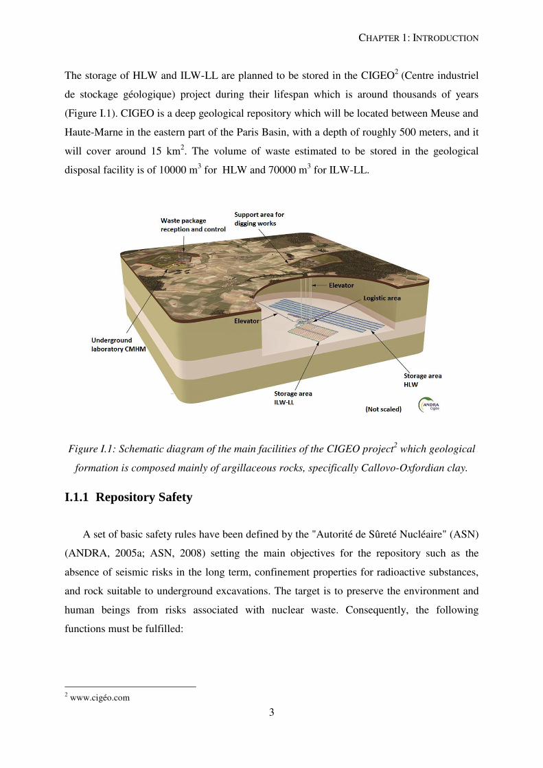
Figure I.1: Schematic diagram of the main facilities of the CIGEO project2 which geological
formation is composed mainly of argillaceous rocks, specifically Callovo-Oxfordian clay. .... 3
Figure I.2: Disposal container for intermediate-level long-lived waste (ILW-LL) containing
four primary waste packages (ANDRA, 2005b). ........................................................................ 5
Figure I.3: Molar fraction of the chemical species H2CO3, HCO3-, and CO3
2- respect pH at
20°C and equilibrium (Thiery, 2006). ....................................................................................... 6
Figure I.4: Carbonation front in a simplified 1D model sketch. Three zones from left to right
can be observed: a fully carbonated concrete with a pH around 9, a transition area where the
carbonation process is occurring and an uncarbonated area with a pH around 13 (Ta et al.,
2016). .......................................................................................................................................... 7
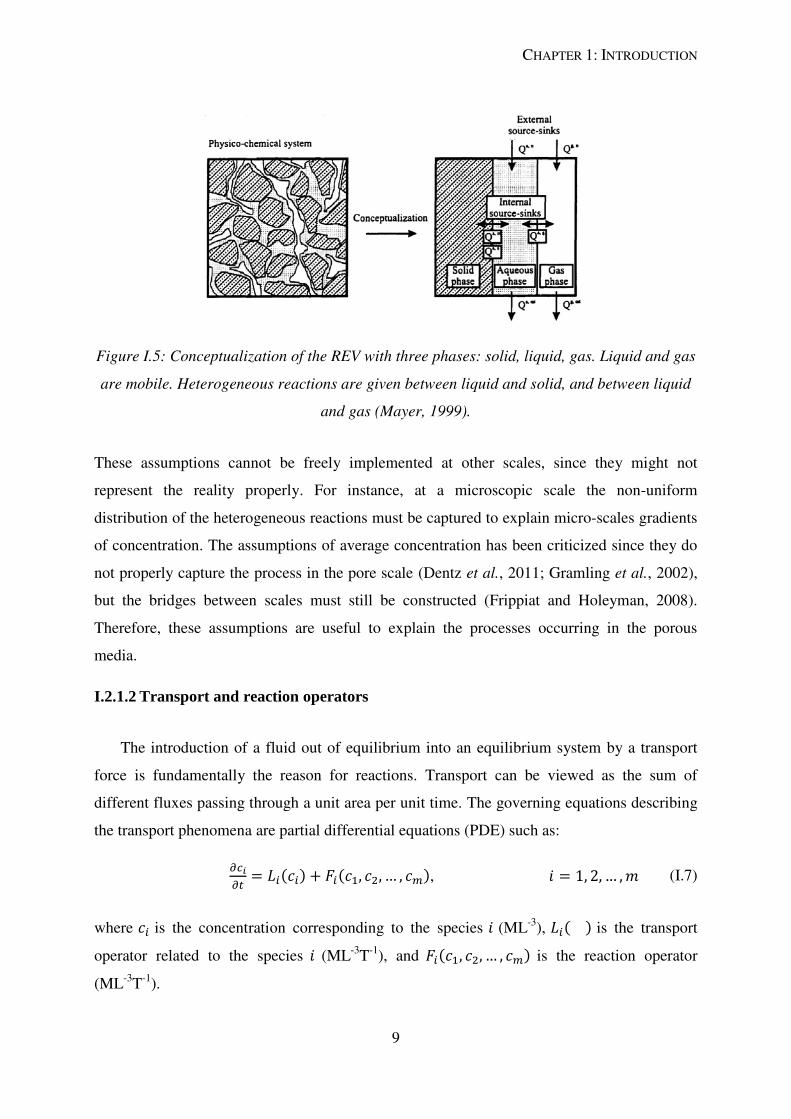
Figure I.5: Conceptualization of the REV with three phases: solid, liquid, gas. Liquid and gas
are mobile. Heterogeneous reactions are given between liquid and solid, and between liquid
and gas (Mayer, 1999). .............................................................................................................. 9
Figure II.1: Transport benchmark parameters and sketch. D is the dispersion coefficient, v is
the velocity, Co are the initial conditions in the 1D column, Ci is the Dirichlet boundary
condition, xmax is the length of the column, ∆t is the splitting time step and ∆x is the spatial
discretization step. .................................................................................................................... 65
Figure II.2: Concentration vs. distance at t = 400 of the different software and analytical
solution for the transport validation benchmark. ..................................................................... 66
Figure II.3: a) Component concentration vs length at time t = 3.6 h, b) concentration at the
end of the column vs time. The results of PHREEQC are represented by a solid line, while the
results of the coupling between FVTool and iPhreeqc are given by empty triangles.. ............ 68
Figure II.4: Concentration vs length plots at a) t = 100 h and b) t = 200 h. The analytical
solution is depicted by a solid line, in the legend it is accompanied by a R. The numerical
solution is depicted by an empty triangle, in the legend accompanied by 'OS' (operator
splitting). The numerical approach used is the additive splitting... ........................................ 71
x
Figure II.5: Time performance comparison of different software coupling with PHREEQC.
External stands for loose coupling between PHREEQC and Python, Dll stands for Python and
iPhreeqc dynamic library, COM stands for Python and iPhreeqc Microsoft component object,
CPP stands for C++ with the dynamic library, and direct stands for PHREEQC alone
(Müller et al., 2011).... ............................................................................................................. 78
Figure III.1: Floor plan view of the concrete structure containing four primary ILW-LL
(ANDRA, 2005) ........................................................................................................................ 87
Figure III.2: Typical capillary pressure- water saturation curve (Hassanizadeh et al., 2002)
.................................................................................................................................................. 92
Figure III.3: 1D domain sketch and boundary conditions for the constant saturation test. .. 100
Figure III.4: Dissolution and precipitation fronts due to carbonation for the initial minerals,
test with constant saturation, Sl = 0.802. ............................................................................... 102
Figure III.5: Aqueous components concentrations and pH, test with constant saturation,
Sl=0.802. ................................................................................................................................ 103
Figure III.6: Dissolution and precipitation fronts due to carbonation for the initial minerals,
test with constant saturation, Sl = 0.602. ............................................................................... 105
Figure III.7: a) amorphous ferrihydrate precipitation, b) pH in the solution. ...................... 106

xi
List of Tables
Table I-1: Families of concrete hydration products. ................................................................. 7
Table II-1: Time performance of the different software for the transport validation
benchmark. ............................................................................................................................... 65
Table II-2: Error comparison between software and analytical solution for the transport
validation benchmark. .............................................................................................................. 66
Table II-3: Physical parameters for the cation exchange benchmark. v is the average velocity,
D is the dispersion coefficient, xmax is the maximum length of the column, ∆x is the grid size,
and ∆t is the time step. ............................................................................................................. 67
Table II-4: Cation exchange benchmark initial and boundary values for aqueous components.
X indicates an exchange site with negative charge. ................................................................. 67
Table II-5: Error of equation ((18) in section II.1) for the " Ca" component with
different OS methods and splitting time steps for the cation exchange benchmark, taking
Strang method with ∆t = 90 s as reference. ............................................................................. 69
Table II-6: Physical and chemical parameters for the multispecies sorption and decay
benchmark. is the average velocity, D is the dispersion coefficient, xmax is the maximum
length of the column, ∆x is the grid size, ∆t is the time step, Kd is the adsorption coefficient,
and ki with i = 1,2, 3 are the reaction rates. ............................................................................ 70
Table II-7: Implementation of boundary conditions in the pdepe built-in function of MATLAB
(Shafei, 2012). .......................................................................................................................... 74
Table II-8: PHREEQC main types of geochemical predefined equations. .............................. 77
Table III-1: initial composition of the concrete package.. ....................................................... 88
Table III-2: Initial aqueous components and its associated primary species according to the
thermochimie database version 8... .......................................................................................... 88
Table III-3: Mineral secondary phases.... ................................................................................ 89
xii
Table III-4: Physical parameters used in the constant saturation test..... ............................... 98
Table III-5: Components initial concentration, plus pH and pe, for the constant saturation
test...... ...................................................................................................................................... 99
Table III-6: Mineral phases initial values for the constant saturation test ............................. 99
Table III-7: Splitting time step due to Von Neumann criteria. is the liquid saturation, is the effective diffusion of vapor and ∆t is the splitting time step. ............................ 100
1
CHAPTER 1: INTRODUCTION
2
I INTRODUCTION
Hydro-chemical numerical simulations are important to assess the safety of disposal
systems for radioactive waste and spent nuclear fuel in deep geological repositories. They
study the different coupled effects between fluid transport (single- and multi-phase) and the
chemical reactions (homogeneous and heterogeneous), and to predict the future
hydro-chemical states over time for the system under study. This field of science is known as
reactive transport modeling and has been applied successfully in different areas such as water
treatment (Langergraber and Šimůnek, 2012), mining industry (Amos et al., 2004), or
geothermal energy (Bozau and van Berk, 2013). Nuclear waste agencies are interested in the
potential of reactive transport modeling to capture the non linear behavior of aqueous
components as a consequence of chemical reactions such as complex aqueous speciation and
kinetically controlled dissolution or precipitation processes.
The thesis is organized into two main sections. The first one is devoted to the development of
a tool that can help to model and gain a deeper insight in the different problems related to
nuclear waste from the point of view of reactive transport modeling in porous media. The
second part frames the problematic of the atmospheric carbonation in the nuclear waste
storage context by using the developed tool.
I.1 Context of the thesis
In France, "L'Agence Nationale pour la gestion des Déchets RadioActifs" (ANDRA1) is
responsible for managing the nuclear waste. The radiological risk of the nuclear waste is
assessed by two parameters: a) the activity level and b) the half-life, originating several
categories of nuclear waste. The activity level is divided into very low, low, intermediate and
high, while the half-life category is divided into very short-lived (less than 100 days),
short-lived (less than 31 years) and long-lived radionuclides (more than 31 years). Two of
these categories are of special interest: the high-level waste (HLW) and the intermediate-level
long-lived waste (ILW-LL). The first one represents around 0.2% of the volume and 96% of
the radioactivity of the nuclear waste and the second around 3% and 4% respectively (Dupuis
and Gonnot, 2013).
1 www.andra.fr
CHAPTER 1: INTRODUCTION
3
The storage of HLW and ILW-LL are planned to be stored in the CIGEO2 (Centre industriel
de stockage géologique) project during their lifespan which is around thousands of years
(Figure I.1). CIGEO is a deep geological repository which will be located between Meuse and
Haute-Marne in the eastern part of the Paris Basin, with a depth of roughly 500 meters, and it
will cover around 15 km2. The volume of waste estimated to be stored in the geological
disposal facility is of 10000 m3 for HLW and 70000 m
3 for ILW-LL.
Figure I.1: Schematic diagram of the main facilities of the CIGEO project2 which geological
formation is composed mainly of argillaceous rocks, specifically Callovo-Oxfordian clay.
I.1.1 Repository Safety
A set of basic safety rules have been defined by the "Autorité de Sûreté Nucléaire" (ASN)
(ANDRA, 2005a; ASN, 2008) setting the main objectives for the repository such as the
absence of seismic risks in the long term, confinement properties for radioactive substances,
and rock suitable to underground excavations. The target is to preserve the environment and
human beings from risks associated with nuclear waste. Consequently, the following
functions must be fulfilled:
2 www.cigéo.com
CHAPTER 1: INTRODUCTION
4
Preventing water circulation because it can degrade waste packages and migration of
radionuclides into the environment;
Limiting the release of radioactive substances by the package and immobilizing them
in the repository as long as possible;
Delaying and reducing the migration of radioactive substances beyond the repository
or geological layer.
In order to complete such functions a passive engineered barrier system is designed
comprising a variety of sub-systems: canister, buffer, backfill, and so on. The main purpose of
such systems is to delay as much as possible the release of radionuclides from the waste to the
host rock. Consequently, ANDRA and homologues institution of other countries (e.g. SKB)
facing similar problems have developed R&D programs to study the behavior of rocks and
radionuclides in order to assess the design of future repositories. Among these studies is
possible to find problems related to the migration of radionuclides such as uranium through
the host rock using experiments or numerical simulations (Dittrich and Reimus, 2015;
Pfingsten, 2014; Xiong et al., 2015). Studies focused on HLW which will be confined in a
vitrified glass either in contact with a bentonite buffer or with the host rock. Consequently, the
evolution of the dissolution of the vitrified glass has been estimated through numerical and
experimental simulations (Debure et al., 2013), and also the interaction between the glass and
bentonite, and between the glass and the host rock through numerical simulations (Ngo et al.,
2014). Numerical experiences have also contributed to give insights on the geochemical
evolution of the HLW, engineered barriers and host rock through the several thousand of
years (Trotignon et al., 2007; Yang et al., 2008), in some cases taking into account possible
climate change scenarios (Nasir et al., 2014; Spycher et al., 2003), or comparing with
analogous natural sites (Chen et al., 2015; Martin et al., 2016). Since many of these studies
have been carried out using or relying on numerical simulations and no analytical solutions
exist, code intercomparison work has also been performed in order to compare codes results
(Marty et al., 2015; Xie et al., 2015).
Here we aim on solving numerical simulations about the effects of atmospheric carbonation
process over concrete in a nuclear waste context.
CHAPTER 1: INTRODUCTION
5
I.1.2 Description of the problem: Atmospheric carbonation
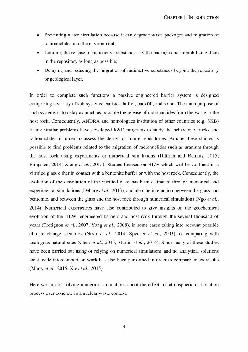
ILW-LL is proposed to be conditioned in cylinders of bitumen or concrete according to
the type of waste which includes metals (fuel claddings), effluent treatment sludges and
nuclear plant operating equipment. The primary ILW-LL package will be placed in a
high-performance reinforced concrete container (Figure I.2), containing from 1 to 4 primary
packages (ANDRA, 2005a; ANDRA, 2005b).
Figure I.2: Disposal container for intermediate-level long-lived waste (ILW-LL) containing
four primary waste packages (ANDRA, 2005b).
The disposal containers of ILW-LL are planned to be placed in vaults which will be ventilated
during the operation period (up to 150 years). Ventilation is required to guarantee operating
safety, evacuate radioactive gas such as hydrogen produced by radiolysis, and residual heat
from the waste. One of the consequences of the vault ventilation is that it will desaturate the
disposal container, leading to a physico-chemical process known as concrete atmospheric
carbonation (Thouvenot et al., 2013).
The atmospheric carbonation process is summarized as follows:
1. The carbon dioxide (CO2) diffuses into the concrete and dissolves into the pore
solution:
. (I.1)
CHAPTER 1: INTRODUCTION
6
2. The water molecules react with CO2 to form carbonic acid (H2CO3):
. (I.2)
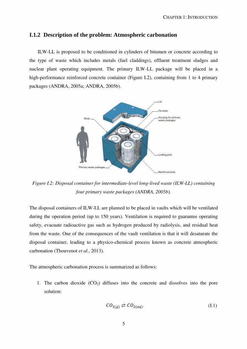
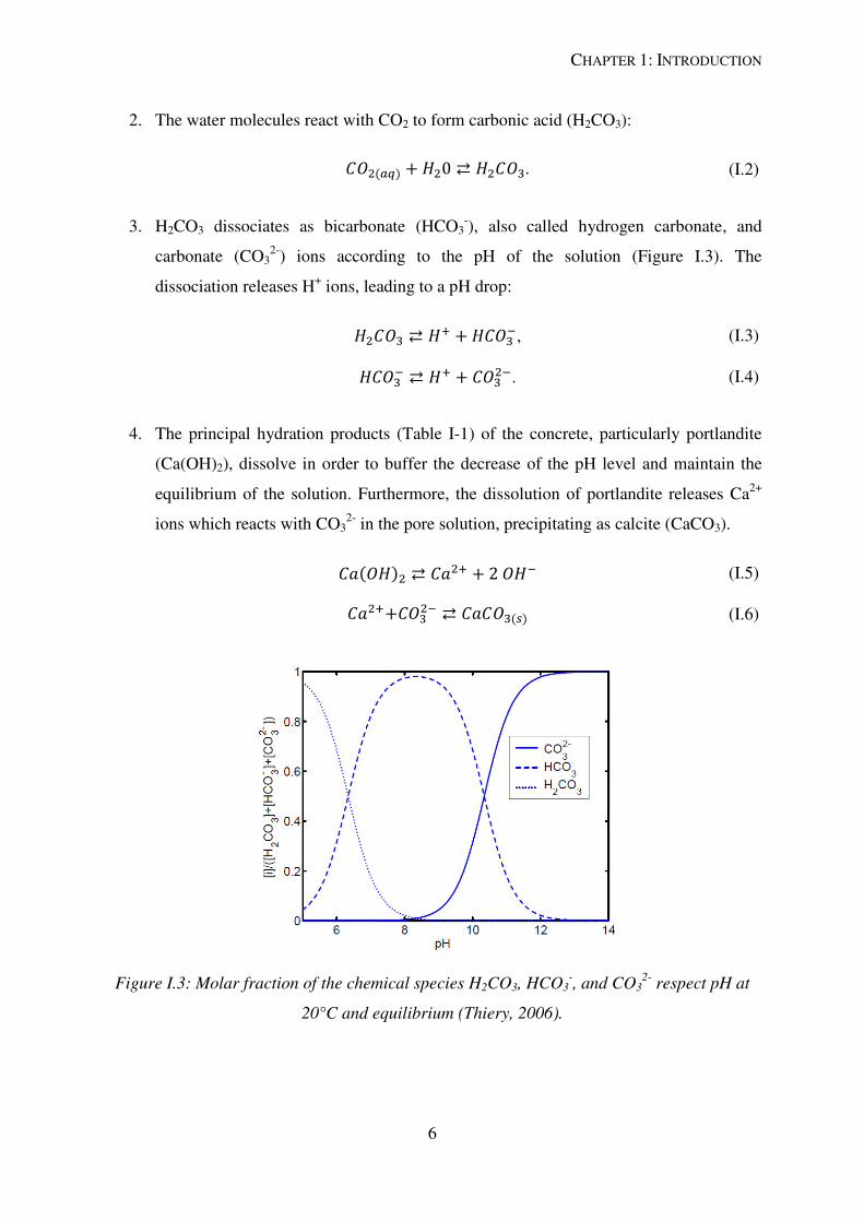
3. H2CO3 dissociates as bicarbonate (HCO3-), also called hydrogen carbonate, and
carbonate (CO32-
) ions according to the pH of the solution (Figure I.3). The
dissociation releases H+ ions, leading to a pH drop:
, (I.3)
. (I.4)
4. The principal hydration products (Table I-1) of the concrete, particularly portlandite
(Ca(OH)2), dissolve in order to buffer the decrease of the pH level and maintain the
equilibrium of the solution. Furthermore, the dissolution of portlandite releases Ca2+
ions which reacts with CO32-
in the pore solution, precipitating as calcite (CaCO3).
(I.5)
(I.6)
Figure I.3: Molar fraction of the chemical species H2CO3, HCO3-, and CO3
2- respect pH at
20°C and equilibrium (Thiery, 2006).

CHAPTER 1: INTRODUCTION
7
Families of
hydration
products
Calcium silicate hydrate (e.g. CSH), Calcium hydroxide (e.g. portlandite), Afm
(e.g. Monocarboaluminate), and AFt (e.g. Ettringite)
Table I-1: Families of concrete hydration products.
At first glance, the carbonation process might not seem harmful for the concrete. Generally,
even a decrease in porosity can be expected because the carbonation products usually have
higher molar volume than their reactants (Glasser et al., 2008). Nevertheless, the decrease in
alkalinity turns out to be an issue for the reinforcing steel bars of the concrete, and thus for the
concrete structure. Normally, the pore solution in concrete has an alkaline environment with a
pH between 12.5 and 13.5 in order to maintain the corrosion of the reinforcing steel bars in a
range of very low rates. At such high pH a thin passive oxide layer forms on the steel and
slows down the corrosion. If the passive layer is destroyed, for example due to the decrease of
pH owing to atmospheric carbonation, corrosion occurs and might result in a failure of the
structure (Zhang, 2016). Therefore, assessing the depth of the carbonation front is a main
mean for evaluating the safety of the concrete package for ILW-LL (Figure I.4).
Figure I.4: Carbonation front in a simplified 1D model sketch. Three zones from left to right
can be observed: a fully carbonated concrete with a pH around 9, a transition area where the
carbonation process is occurring and an uncarbonated area with a pH around 13 (Ta et al.,
2016).
CHAPTER 1: INTRODUCTION
8
Experimental studies of the carbonation process give an insight of the phenomenon in the
concrete package (Duprat et al., 2014; Ekolu, 2016; Shi et al., 2016; Thiery et al., 2007), but
due to the long time scale of the waste confinement, detailed numerical studies of the
physico-chemical processes are necessary in order to assess the safety of the disposal
containers.
I.2 State-of-the-art: Reactive transport modeling
I.2.1 Mathematical model
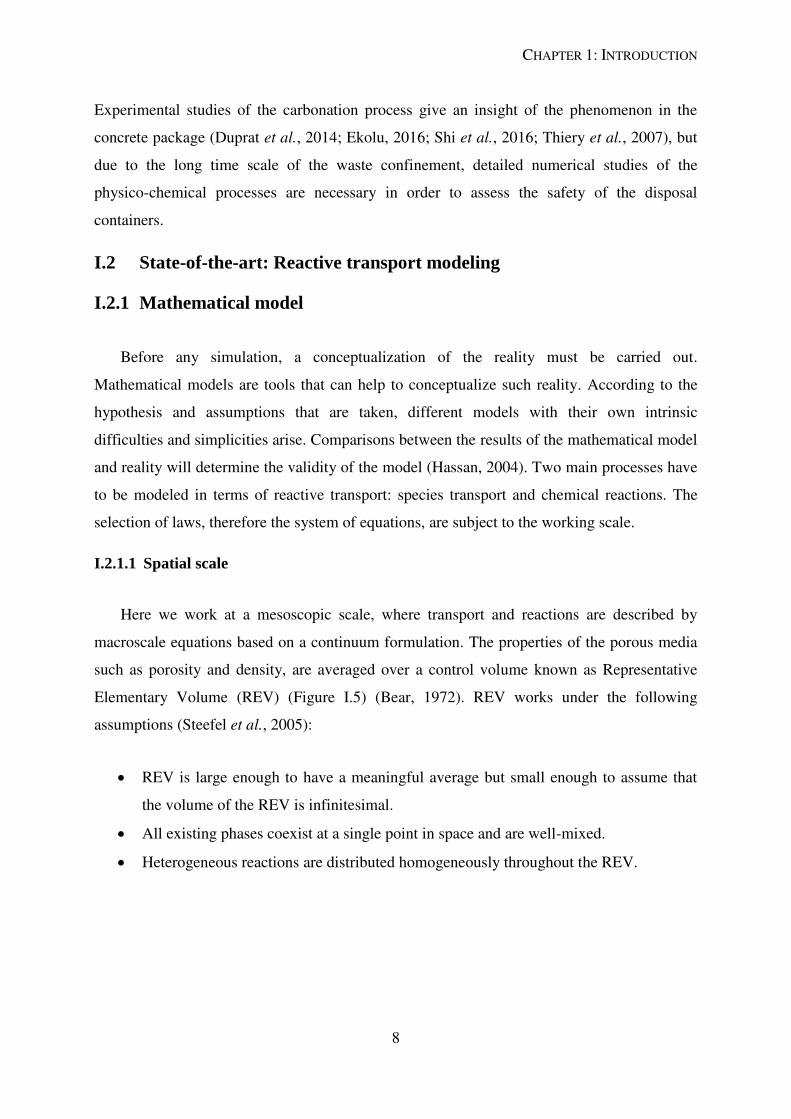
Before any simulation, a conceptualization of the reality must be carried out.
Mathematical models are tools that can help to conceptualize such reality. According to the
hypothesis and assumptions that are taken, different models with their own intrinsic
difficulties and simplicities arise. Comparisons between the results of the mathematical model
and reality will determine the validity of the model (Hassan, 2004). Two main processes have
to be modeled in terms of reactive transport: species transport and chemical reactions. The
selection of laws, therefore the system of equations, are subject to the working scale.
I.2.1.1 Spatial scale
Here we work at a mesoscopic scale, where transport and reactions are described by
macroscale equations based on a continuum formulation. The properties of the porous media
such as porosity and density, are averaged over a control volume known as Representative
Elementary Volume (REV) (Figure I.5) (Bear, 1972). REV works under the following
assumptions (Steefel et al., 2005):
REV is large enough to have a meaningful average but small enough to assume that
the volume of the REV is infinitesimal.
All existing phases coexist at a single point in space and are well-mixed.
Heterogeneous reactions are distributed homogeneously throughout the REV.
CHAPTER 1: INTRODUCTION
9
Figure I.5: Conceptualization of the REV with three phases: solid, liquid, gas. Liquid and gas
are mobile. Heterogeneous reactions are given between liquid and solid, and between liquid
and gas (Mayer, 1999).
These assumptions cannot be freely implemented at other scales, since they might not
represent the reality properly. For instance, at a microscopic scale the non-uniform
distribution of the heterogeneous reactions must be captured to explain micro-scales gradients
of concentration. The assumptions of average concentration has been criticized since they do
not properly capture the process in the pore scale (Dentz et al., 2011; Gramling et al., 2002),
but the bridges between scales must still be constructed (Frippiat and Holeyman, 2008).
Therefore, these assumptions are useful to explain the processes occurring in the porous
media.
I.2.1.2 Transport and reaction operators
The introduction of a fluid out of equilibrium into an equilibrium system by a transport
force is fundamentally the reason for reactions. Transport can be viewed as the sum of
different fluxes passing through a unit area per unit time. The governing equations describing
the transport phenomena are partial differential equations (PDE) such as:
, (I.7)
where is the concentration corresponding to the species (ML-3
), is the transport
operator related to the species (ML-3
T-1
), and is the reaction operator
(ML-3
T-1
).
CHAPTER 1: INTRODUCTION
10
Transport
The transport operator is composed by an advection and diffusion-dispersion term, and is
given by:
, (I.8)
where is the velocity vector (LT-1
) and the diffusion-dispersion tensor (L2T
-1) (Bear,
1972; Scheidegger, 1954).
Advection
The advection is the translation in space of a substance by bulk motion. In the reactive
transport field, advection has been usually modeled by applying Darcy's law. Darcy
discovered that there was a relationship between the flow rate of a liquid flowing through a
porous media and the gradient of pressures (Darcy, 1856). Later, a mathematical expressions
were derived from the Navier-Stokes equation (Hubbert, 1957; Whitaker, 1986) which
corroborates the relationship of Darcy. Darcy's law for single phase flow is given by:
, (I.9)
where is the absolute (or intrinsic) permeability tensor (L2) which is a characteristic
property of the solid matrix, is the dynamic viscosity (MT-1
L-1
), is the gravity vector
(LT-2
), is the pressure (MT-2
L-1
), is density of the α phase (ML-3
), and is the volumetric
fluid velocity (LT-1
). Darcy law might not be the first option if the fluid in the porous media is
fast, since the pressure drops induced by inertial effects are not well capture by Darcy's law
(Veyskarami et al., 2016).
Diffusion
Diffusion is the concentration flux induced by concentration gradients. It has usually been
modeled by application of Fick's law (Fick, 1855):
, (I.10)

CHAPTER 1: INTRODUCTION
11
where is the molecular diffusion (L2T
-1). In porous media, the molecular diffusion of
equation (I.10) is replaced by an effective diffusion. It is derived from the molecular diffusion
to take into account the influence of the geometry of the porous media:
, (I.11)
where is the effective diffusion coefficient (L2T
-1), is the tortuosity of the porous media
(-), and is the liquid volume fraction (-). Application of Fick's law might be controversial in
some situations, such as in the case where the solution is not diluted and is charged (Steefel
and Maher, 2009). Diffusion is species dependent, but in some cases it can be considered
equal to all the species in the same phases. For example, in advection-dominated case.
Dispersion
Hydrodynamical dispersion is caused by the fact that groundwater must flow around solid
particles (porous medium). Consequently, the diverging path of water will cause variations in
velocity within pore channels leading to solute spreading, such mechanical mixing is called
dispersion. The dispersion tensor is normally calculated from the velocity field of the fluid ,
for instance in a 1D case:
, (I.12)
where is the dispersivity (L), and DD the dispersion tensor (L2T
-1). The sum of the
dispersion and diffusion turns out to give the dispersion-diffusion tensor.
The dispersion-diffusion tensor can be estimated from a Fickian dispersion or a non-Fickian
dispersion. The first has a dispersivity which is spatial-dependent (Burnett and Frind, 1987),
whereas the second might depend on time (Zoua et al., 1996) or other parameters.
This section has introduced basic transport fluxes, but other forces can have a significant role.
For instance, geochemical reactions have an impact on flow properties such as viscosity and
density (Abriola and Pinder, 1985; Wissmeier and Barry, 2008), also they can modified the
porosity of the solid matrix due to precipitation/dissolution processes, affecting the
permeability parameter (Cochepin et al., 2008; Dobson et al., 2003; Poonoosamy et al.,
2015).
CHAPTER 1: INTRODUCTION
12
Chemistry
Chemical reactions transform a set of chemical substances (reactants) into another (products).
They are modeled using fundamentally two mathematical descriptions: equilibrium reactions
through the Local Equilibrium Assumption (LEA) (Thompson, 1959) and kinetic reactions.
The first one is represented by algebraic equations (AEs) and the second one by Ordinary
Differential Equations (ODEs) (Rubin, 1983). Reactions that occur in the same phase are
known as homogeneous reactions, whereas reactions that involve mass transfer between
different phases are known as heterogeneous reactions. Some of the most common reactions
that can be found are (Merkel et al., 2005):
Aqueous complexation (Speciation).
Redox processes.
Dissolution/Precipitation.
Surface complexation.
Gas-liquid interactions.
The choice of whether to model a reaction as kinetic or equilibrium is given by its
characteristic time scale. In Steefel and Maher (2009) it is stated that if the Damköhler
number is significantly larger than one, the reaction which is taking place is faster than the
transport time scale, hence the hypotheses of the equilibrium approach is assumed valid. For
example, reactions such as aqueous complexation are extremely fast, hence they are usually
modeled as equilibrium reactions. Other reactions, like rusting, are slow, therefore a kinetic
approach would be more appropriate.
Equilibrium reactions
The equilibrium state is the most stable state of a chemical system for a given set of state
variables such as temperature (T), pressure (P), and compositional constraints. The chemical
state is defined by the total Gibbs free energy (G), and its differential changes with the
progress variable which is the number of moles of a reactant normalized to the
stoichiometric coefficient (Nordstrom, 2004):
. (I.13)
CHAPTER 1: INTRODUCTION
13
Any perturbation in the system will force equation (I.13) to be different than 0. Consequently,
after a perturbation the new minimum in the free-energy curve must be found so as to know
the new equilibrium state. There are two main approaches to solve the problem: a) The
equilibrium constant approach (Brinkley 1947; Morel and Morgan, 1972) based on the ion
association theory (Bjerrum, 1926) and the free-energy minimization approach (Van Zeggeren
and Storey, 2011; White et al., 1958) based on the mixed electrolyte theory (Reilly et al.,
1971). Both approaches employ mass-balance and mass-action laws. They are related by:
, (I.14)
where is the universal gas constant (L2T
-2 ϴ-1
), is the absolute temperature (ϴ), is the
equilibrium constant, and is Gibbs free energy of the reaction (ML2T
-2).
Although both approaches should give the same results, their implemented solution might
differ. Thus, the free-energy minimization approach uses a minimization procedure which is
not mathematically equivalent to find the roots of a set of nonlinear algebraic equations,
which is the method used by the equilibrium constant approach (Press et al., 2007).
Furthermore, the free energy minimization approach relaxes the equilibrium states of the
system while keeping the mass balance fixed. Mass is gradually adjusted until the equilibrium
of the system is achieved. On the other hand, the equilibrium constant approach relaxes the
mass balance while keeping the equilibrium constant fixed. So, during the iterations of the
numerical technique the mass balance is gradually adjusted until the specified convergence is
reached. If there are large mass balance violations, the problem does not converge (Steefel
and MacQuarrie, 1996).
Mass action law
Chemical equilibrium reactions can be mathematical described by a mass balance equation
such as:
, (I.15)
where is the stoichiometric coefficient of species i for the j reaction. The number of
products and reactant varies according to the reaction in consideration. Note that the equation
CHAPTER 1: INTRODUCTION
14
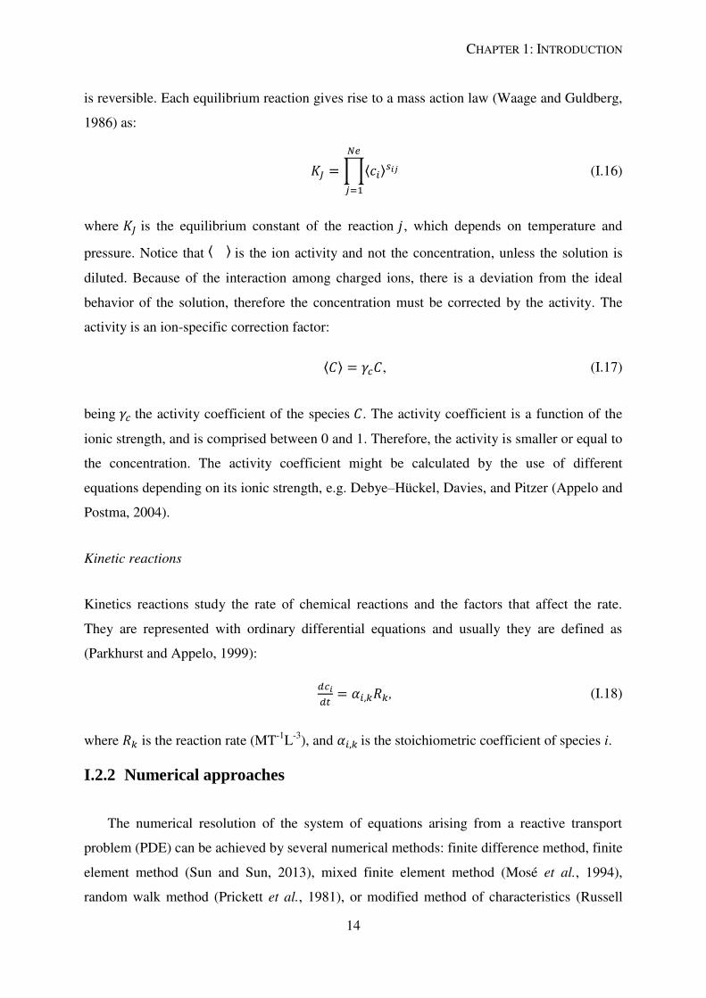
is reversible. Each equilibrium reaction gives rise to a mass action law (Waage and Guldberg,
1986) as:
(I.16)
where is the equilibrium constant of the reaction , which depends on temperature and
pressure. Notice that is the ion activity and not the concentration, unless the solution is
diluted. Because of the interaction among charged ions, there is a deviation from the ideal
behavior of the solution, therefore the concentration must be corrected by the activity. The
activity is an ion-specific correction factor:
, (I.17)
being the activity coefficient of the species . The activity coefficient is a function of the
ionic strength, and is comprised between 0 and 1. Therefore, the activity is smaller or equal to
the concentration. The activity coefficient might be calculated by the use of different
equations depending on its ionic strength, e.g. Debye–Hückel, Davies, and Pitzer (Appelo and
Postma, 2004).
Kinetic reactions
Kinetics reactions study the rate of chemical reactions and the factors that affect the rate.
They are represented with ordinary differential equations and usually they are defined as
(Parkhurst and Appelo, 1999):
, (I.18)
where is the reaction rate (MT-1
L-3
), and is the stoichiometric coefficient of species i.
I.2.2 Numerical approaches
The numerical resolution of the system of equations arising from a reactive transport
problem (PDE) can be achieved by several numerical methods: finite difference method, finite
element method (Sun and Sun, 2013), mixed finite element method (Mosé et al., 1994),
random walk method (Prickett et al., 1981), or modified method of characteristics (Russell

CHAPTER 1: INTRODUCTION
15
and Wheeler, 1983). A table with some methods can be found in Besnard (2004). Here we do
not focus on the numerical methods but rather on the numerical approach.
In the field of reactive transport two main approaches exist: operator splitting or global
implicit approach. The operator splitting follows a "divide and conquer" strategy by
decoupling the system (Holden et al., 2010), and then solving each part of the governing
equations separately (Engesgaard and Kipp, 1992). On the other hand, global implicit
approach solves simultaneously the governing equations of transport and chemistry leading to
a fully coupled system (de Dieuleveult and Erhel, 2010). Both methods have their advantages
and drawbacks. Operator splitting can be easily implemented, it can use existing geochemical
or nonreactive transport software (Parkhurst et al., 2004), each operator can be solved with
the most suitable technique. Unfortunately, the decoupling of operators leads, in general, to
the splitting error (Carrayrou et al., 2004). Iterative approaches might be used to reduce such
error, but convergence problems might arise (Samper et al., 2000). On the other hand, global
implicit approaches are more difficult to implement due to larger and more complex systems
and require more computational resources, however they are more robust and accurate
(Saaltink et al., 2000).
During several decades the only plausible scheme to solve a large set of equations was the
operator splitting approach (Yeh and Tripathi, 1989). Once the computational power of
computers increased, studies have shown the benefits of the global implicit approaches (Fahs
et al., 2008; Saaltink et al., 2001). Nowadays, thanks to more refined numerical formulations
(Hoffmann et al., 2012; Molins et al., 2004), high performance computation (Glenn et al.,
2007; Hoffmann et al., 2010), and new numerical schemes (Hammond et al., 2005), the gap
between the efficiency of global implicit and operator splitting seems to be closed (Carrayrou
et al., 2010).
I.2.3 Codes
The number of reactive transport codes in literature is large. Tables describing some of
these codes can be found in Carrayrou et al. (2010), Steefel et al. (2015), Sedighi (2011), and
Lee et al. (2011). The codes are based on two of the previous strategies although each one has
its own particularities. For instance, Crunchflow (Steefel, 2009) and MIN3P (Mayer, 2000)
are two codes that use global implicit approach but the amount of physical phenomena that
CHAPTER 1: INTRODUCTION
16
they can reproduce is not the same, since Richards' equation for unsaturated soil can be solved
in MIN3P but not in Crunchflow. Also, Crunchflow is not parallelized, contrary to MIN3P.
Nevertheless, Crunchflow can also work using splitting operator approaches and MIN3P
cannot. Other codes with similar strategies (operator splitting approach) are HP1 (Jacques and
Šimůnek, 2005) and PHT3D (Appelo and Rolle, 2010), but each one has its own features.
HP1 discretizates its space using finite element method, whereas PHT3D uses finite volume
method as well as a modified method of characteristics.
The difference between codes do not only reside on its computational efficiency, numerical
techniques or implemented phenomena. The distribution policy of each software can also
differ. Software like OpenGeoSys (Kolditz et al., 2012) and PFLOTRAN (Lichtner et al.,
2015) are open source making it available to everyone, while others such as Hytec (van der
Lee et al., 2003) and Toughreact (Xu et al., 2011) are commercial software.
In general, all the software tend to embed the transport and chemical operators which may
difficult the application of new numerical methods and schemes. In order to gain flexibility,
we propose an object-oriented approach using operator splitting techniques in a generic form,
allowing users to develop new decoupled schemes and to plug their different transport and
chemistry solvers in an open source environment.
I.3 Objectives and issues
The motivation of this thesis arises from the problematic of modeling atmospheric
carbonation on a concrete overpack for ILW-LL by applying operator splitting methods in the
field of reactive transport modeling. Simulation of carbonation process can be found in the
literature but they are rather simplified systems (Bary and Mügler, 2006). These simplified
problems help to understand main key parameters such as the role of the aggregates in the
carbonation process (Ruan and Pan, 2012), the width of the carbonation front associated to the
characteristic time of the chemical reactions of carbonation and to the characteristic time of
the CO2 diffusion (Thiery et al., 2007), the impact of the carbonated zones in the moisture,
and the transport of gaseous CO2 and calcium ions (Bary and Sellier, 2004). Although,
complex chemical system which might help to understand the detailed chemical evolution of
the solid matrix are rather scarce (Trotignon et al., 2011). Rather than focus only in the
physical and chemical process, we analyze operator splitting approaches in practical cases by
CHAPTER 1: INTRODUCTION
17
solving each physico-chemical phenomena with different solvers such as COMSOL and
PHREEQC. To find about new possible approaches to solving the carbonation process.
However, the separation of process in order to solve the system of interest might lead to an
error, since the approach usually decouples non-linear systems (Carrayrou et al., 2004;
Simpson and Landman, 2008). Therefore a series of questions arise, such as: What are the
tools to understand the operator splitting error? What are the consequence derived from using
different numerical approaches? What limitations arise from operator splitting approach and
from the application of different solvers? And the limiting factors in simulating the
carbonation process by operator splitting techniques? To answer this questions, we implement
a generic operator splitting into a code by using object-oriented programming in order to
couple different solvers of transport and chemistry.
The use of object-oriented programming allows to keep separate processes and to quickly
develop and try new implementations. This separation gives the possibility of explore new
operator splitting algorithms and coupled different solvers in practical cases.
18
CHAPTER 2: DEVELOPMENT OF
TREACLAB
19
II. DEVELOPMENT OF TREACLAB
The following section presents the submitted article which can be read in section II.1,
extra benchmarks (section II.2), extra information of the used codes by TReacLab (section
II.3) and operator splitting concepts related to the article (section II.4). In the article, we
illustrate the different operator splitting methods implemented in the object-oriented code
TReacLab: sequential splitting (Geiser, 2009), alternating additive splitting (Faragó et al.,
2008a; Faragó et al., 2008b), Strang (Strang, 1968) and symmetrically weighted splitting
(Csomós et al., 2005), and also the two sequential iterative approaches: SIA TC and SIA CC
(de Dieuleveult et al., 2009). The schemes are consistent and performances are consistent
with the references, which are mainly analytical solutions and numerical results of the
PHREEQC software. Furthermore, we illustrate the easiness and flexibility of plugging new
solvers into TReacLab, from commercial software like COMSOL, to open source software
like iPhreeqc. Assuming that the reactive transport problem is well-posed, there is a consistent
decomposition of operators and each operator is solved with sufficient accuracy. We would
expect to get the better results with sequential iterative approaches providing that convergence
is reached, followed by the second-order operator splitting: alternating, Strang and
symmetrically weighted splitting, and finally the first-order splitting: sequential and additive
splitting. If the operators of chemistry and transport commute, which is usually not the case,
operator splitting might be as accurate as sequential iterative approaches. In terms of
computation speed, non-iterative approaches are faster, since for each time step there is no
need to iterate (Samper et al., 2009).
CHAPTER 2: DEVELOPMENT OF TREACLAB
20
II.1 Article
TReacLab: an object-oriented implementation of non-intrusive
splitting methods to couple independent transport and geochemical
software

CHAPTER 2: DEVELOPMENT OF TREACLAB
21
TReacLab: an object-oriented implementation of non-intrusive
splitting methods to couple independent transport and geochemical
software
Daniel Jara1, Jean-Raynald de Dreuzy
1, Benoit Cochepin
2
1Géosciences Rennes, UMR CNRS 6118, Campus de Beaulieu, University of Rennes 1,
Rennes, France
2ANDRA, 1/7 Rue Jean Monnet, 92298 Châtenay-Malabry, France
Abstract
Reactive transport modeling contributes to understand geophysical and geochemical processes
in subsurface environments. Operator splitting methods have been proposed as non-intrusive
coupling techniques that optimize the use of existing chemistry and transport codes. In this
spirit, we propose a coupler relying on external geochemical and transport codes with
appropriate operator segmentation that enables possible developments of additional splitting
methods. We provide an object-oriented implementation in TReacLab developed in the
MATLAB environment in a free open source frame with an accessible repository. TReacLab
contains classical coupling methods, template interfaces and calling functions for two
classical transport and reactive software (PHREEQC and COMSOL). It is tested on four
classical benchmarks with homogeneous and heterogeneous reactions at equilibrium or
kinetically-controlled. We show that full decoupling to the implementation level has a cost in
terms of accuracy compared to more integrated and optimized codes. Use of non-intrusive
implementations like TReacLab are still justified for coupling independent transport and
chemical software at a minimal development effort but should be systematically and carefully
assessed.
Keywords: Porous media; Reactive transport; Operator splitting; Object-oriented
programming.
Corresponding author: [email protected]
CHAPTER 2: DEVELOPMENT OF TREACLAB
22
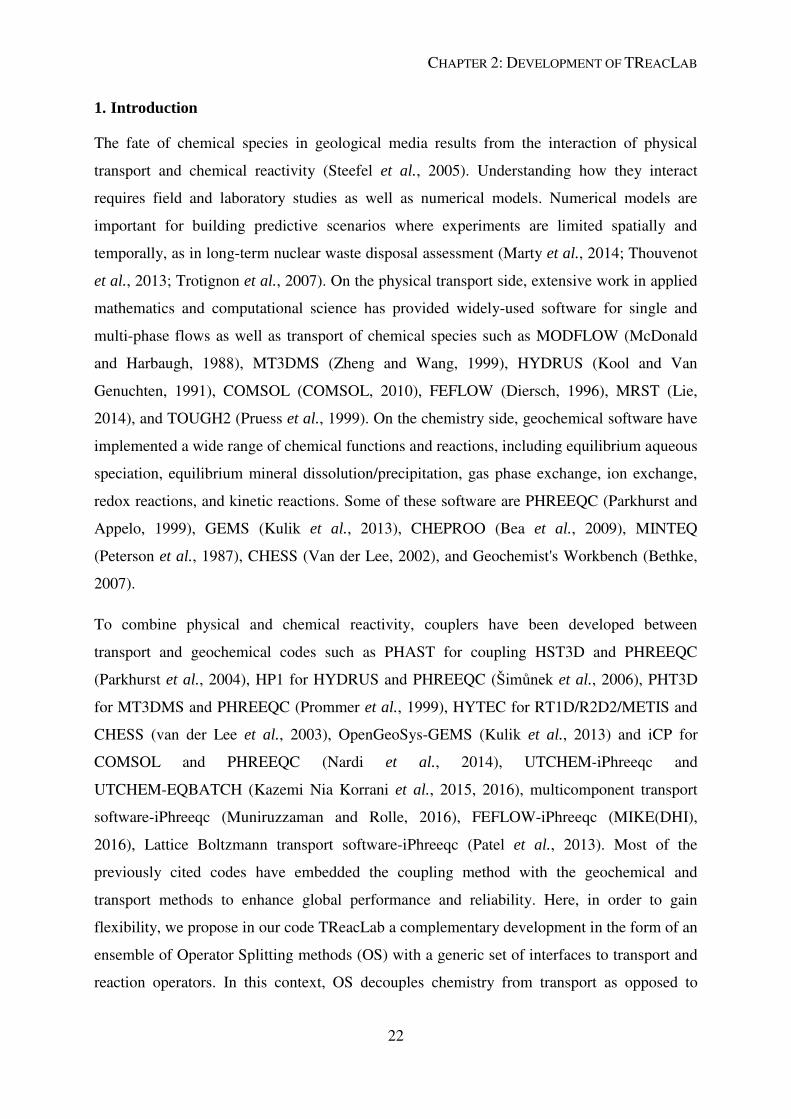
1. Introduction
The fate of chemical species in geological media results from the interaction of physical
transport and chemical reactivity (Steefel et al., 2005). Understanding how they interact
requires field and laboratory studies as well as numerical models. Numerical models are
important for building predictive scenarios where experiments are limited spatially and
temporally, as in long-term nuclear waste disposal assessment (Marty et al., 2014; Thouvenot
et al., 2013; Trotignon et al., 2007). On the physical transport side, extensive work in applied
mathematics and computational science has provided widely-used software for single and
multi-phase flows as well as transport of chemical species such as MODFLOW (McDonald
and Harbaugh, 1988), MT3DMS (Zheng and Wang, 1999), HYDRUS (Kool and Van
Genuchten, 1991), COMSOL (COMSOL, 2010), FEFLOW (Diersch, 1996), MRST (Lie,
2014), and TOUGH2 (Pruess et al., 1999). On the chemistry side, geochemical software have
implemented a wide range of chemical functions and reactions, including equilibrium aqueous
speciation, equilibrium mineral dissolution/precipitation, gas phase exchange, ion exchange,
redox reactions, and kinetic reactions. Some of these software are PHREEQC (Parkhurst and
Appelo, 1999), GEMS (Kulik et al., 2013), CHEPROO (Bea et al., 2009), MINTEQ
(Peterson et al., 1987), CHESS (Van der Lee, 2002), and Geochemist's Workbench (Bethke,
2007).
To combine physical and chemical reactivity, couplers have been developed between
transport and geochemical codes such as PHAST for coupling HST3D and PHREEQC
(Parkhurst et al., 2004), HP1 for HYDRUS and PHREEQC (Šimůnek et al., 2006), PHT3D
for MT3DMS and PHREEQC (Prommer et al., 1999), HYTEC for RT1D/R2D2/METIS and
CHESS (van der Lee et al., 2003), OpenGeoSys-GEMS (Kulik et al., 2013) and iCP for
COMSOL and PHREEQC (Nardi et al., 2014), UTCHEM-iPhreeqc and
UTCHEM-EQBATCH (Kazemi Nia Korrani et al., 2015, 2016), multicomponent transport
software-iPhreeqc (Muniruzzaman and Rolle, 2016), FEFLOW-iPhreeqc (MIKE(DHI),
2016), Lattice Boltzmann transport software-iPhreeqc (Patel et al., 2013). Most of the
previously cited codes have embedded the coupling method with the geochemical and
transport methods to enhance global performance and reliability. Here, in order to gain
flexibility, we propose in our code TReacLab a complementary development in the form of an
ensemble of Operator Splitting methods (OS) with a generic set of interfaces to transport and
reaction operators. In this context, OS decouples chemistry from transport as opposed to
CHAPTER 2: DEVELOPMENT OF TREACLAB
23
global implicit solvers, which have been proven to be more accurate but less flexible
(Hammond et al., 2012; Mayer, 2000; Steefel, 2009; Zhang, 2012). TReacLab is designed as
an open toolbox where additional OS techniques can be implemented and benchmarked.
Other transport and geochemical codes may also be used at the minimal cost of developing
the necessary interfaces. TReacLab is written in MATLAB based on a series of abstract
classes using object-oriented programming (Commend and Zimmermann, 2001; Register,
2007; Rouson et al., 2011).
After recalling in section 2 the reactive transport and OS formalism used, we present in
section 3 our OS implementation. We especially show how to implement alternative OS
methods and how to connect other transport and geochemical codes. Methods are assessed
and discussed on the basis of 3 benchmarks in section 4.
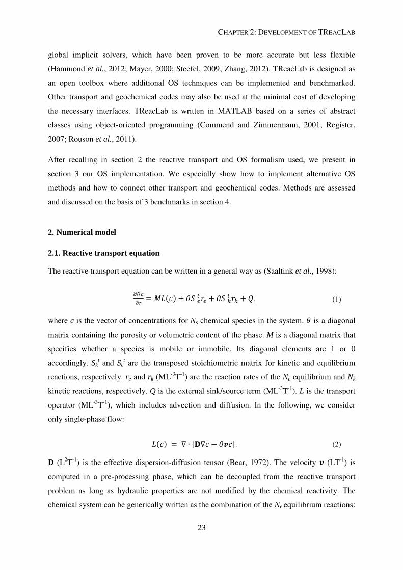
2. Numerical model
2.1. Reactive transport equation
The reactive transport equation can be written in a general way as (Saaltink et al., 1998):
, (1)
where c is the vector of concentrations for Ns chemical species in the system. is a diagonal
matrix containing the porosity or volumetric content of the phase. M is a diagonal matrix that
specifies whether a species is mobile or immobile. Its diagonal elements are 1 or 0
accordingly. Skt and Se
t are the transposed stoichiometric matrix for kinetic and equilibrium
reactions, respectively. re and rk (ML-3
T-1
) are the reaction rates of the Ne equilibrium and Nk
kinetic reactions, respectively. Q is the external sink/source term (ML-3
T-1
). L is the transport
operator (ML-3
T-1
), which includes advection and diffusion. In the following, we consider
only single-phase flow:
. (2) (L2T
-1) is the effective dispersion-diffusion tensor (Bear, 1972). The velocity (LT
-1) is
computed in a pre-processing phase, which can be decoupled from the reactive transport
problem as long as hydraulic properties are not modified by the chemical reactivity. The
chemical system can be generically written as the combination of the Ne equilibrium reactions:
CHAPTER 2: DEVELOPMENT OF TREACLAB
24
, (3)
and of the Nk kinetically-controlled reactions:
. (4)
The reactive transport problem is thus made up of the Ns mass balance equation (1) and of the
Ne + Nk equilibrium and kinetic equations (3) and (4). Its unknowns are the concentrations c
and the reaction rates re and rk. The chemical equilibrium system (3) is composed of the
conservation equation and of the mass action law, relating reactants and products (Apoung-
Kamga et al., 2009; Molins et al., 2004):
, (5)
where K is the vector of equilibrium constants.
Components u are generally introduced when considering equilibrium reactions (Saaltink et
al., 2011):
, (6)
where U is the component matrix (Fang et al., 2003; Friedly and Rubin, 1992; Hoffmann et
al., 2012; Kräutle and Knabner, 2005; Steefel et al., 2005). They are Ns - Ne linear
combinations of chemical species that are not modified by equilibrium reactions (Molins et
al., 2004; Morel and Hering, 1993):
. (7)
The component matrix is not unique. However, its application to equation (1) always leads to
a reduced system without the equilibrium rates but with the components u (Molins et al.,
2004; Saaltink et al., 1998):
. (8)
The reactive transport problem is then made up of the 2Ns - Ne + Nk equations (3-6) and (8)
for the same number of unknowns u, c and rk.
CHAPTER 2: DEVELOPMENT OF TREACLAB
25
Under the assumption that solid species are not transported and all species have the same
diffusion coefficient (i.e. ). Equation (8) classically gives the two following
formulations TC and CC (Amir and Kern, 2010):
TC: . (9)
CC: . (10)
where and are the aqueous and fixed components. In the TC
formulation, the fixed species concentration are deducted from the solution in the total
component concentration (T) and the solute concentration (C). In the CC formulation, the
total component concentration is divided in aqueous and fixed components.
2.2. Usual first-order sequential non-iterative and iterative approaches
In this section, we show how the reactive transport problem can be solved using independent
transport and chemical solvers. We distinguish the sequential non-iterative and iterative
approaches respectively based on TC and CC formulations. For the sequential non-iterative
approach, we extract from the TC formulation, the transport operator in which we keep the
sink/source term:-
. (11)
The chemical operator derives from equations (3-6), and (8). Note that it does not contain any
source/sink term, as it has been included in the transport equation:
(12)
.
This is still a system of 2Ns - Ne + Nk equations for the same number of unknowns. This
decoupled system can be solved with the classical sequential non-iterative approach using an
explicit integration of temporal derivatives (herein, we assume forward Euler). The solution at
CHAPTER 2: DEVELOPMENT OF TREACLAB
26
time step n+1 can be obtained from the solution at time step n, with the following successive
application of the transport and chemical operators in a sequential approach:
(13)
The transport operator (11) is applied to the components. Then the chemical operator is
applied with the updated mobile components for speciation between fixed and solute
concentrations. In the specific case where chemical reactions are all at equilibrium and no
kinetics is involved, a TC formulation is used to fully decouple (de Dieuleveult et al., 2009),
the decoupling does not then rely on operator splitting, but on a block Gauss-Seidel
method.When the stability conditions of the explicit integration are too much constraining,
implicit schemes should be used instead within a sequential iterative approach (Carrayrou et
al., 2004; de Dieuleveult and Erhel, 2010; Yeh and Tripathi, 1989):
(14)
. Classical Picard's method have been extensively used to solve such kind of problems:
(15)
,
where k is the index of the Picard iteration method instantiated by:
(16)
CHAPTER 2: DEVELOPMENT OF TREACLAB
27
.
We recall the necessity to check the consistency of the temporal integration scheme with the
Operator Splitting method chosen. With this decomposition, explicit first-order scheme
naturally leads to sequential non-iterative approach. The implicit first-order scheme requires a
sequential iterative approach. Other choices are possible and might reduce errors depending
on the chemical system (Barry et al., 1996). As it should be possible to test and benchmark
them at a reduced development cost, we use a generic decoupling formalism that can be used
to implement a broad range of schemes.
2.3. Generic operator splitting implementation
The reactive transport system can be generically split in two operators. Using the formalism
of Gasda et al. (2011), equation (1) can be written as:
, , , (17)
where is the unknown, and can be equation (11) and (12), respectively. Other
decomposition are possible, e.g. the transport operator can be subdivided into an advection
and a diffusion-dispersion operator (Clement et al., 1998), or one operator might contain
advection-reaction and the other diffusion (Liu and Ewing, 2005). Each operator will be
solved separately for a splitting time step using adapted numerical methods.
The generic operator splitting methods implemented into the Toolbox are the sequential
splitting, additive splitting, Strang splitting, symetrically weighted splitting, and alternating
method (Appendix A). Assuming exact integration of the operators and homogeneous
boundary conditions in equation (18), the first two have a first-order temporal truncation
error, and the following three a second-order one (Hundsdorfer and Verwer, 2013). Since the
operators are usually solved using numerical methods, the global order of such approaches
might be modified because of the order of the numerical methods used for each operator
(Barry et al., 1996; Csomós and Faragó, 2008). The alternating splitting increases the order of
the sequential splitting if the time steps are small enough (Simpson and Landman, 2008;
Valocchi and Malmstead, 1992).
CHAPTER 2: DEVELOPMENT OF TREACLAB
28
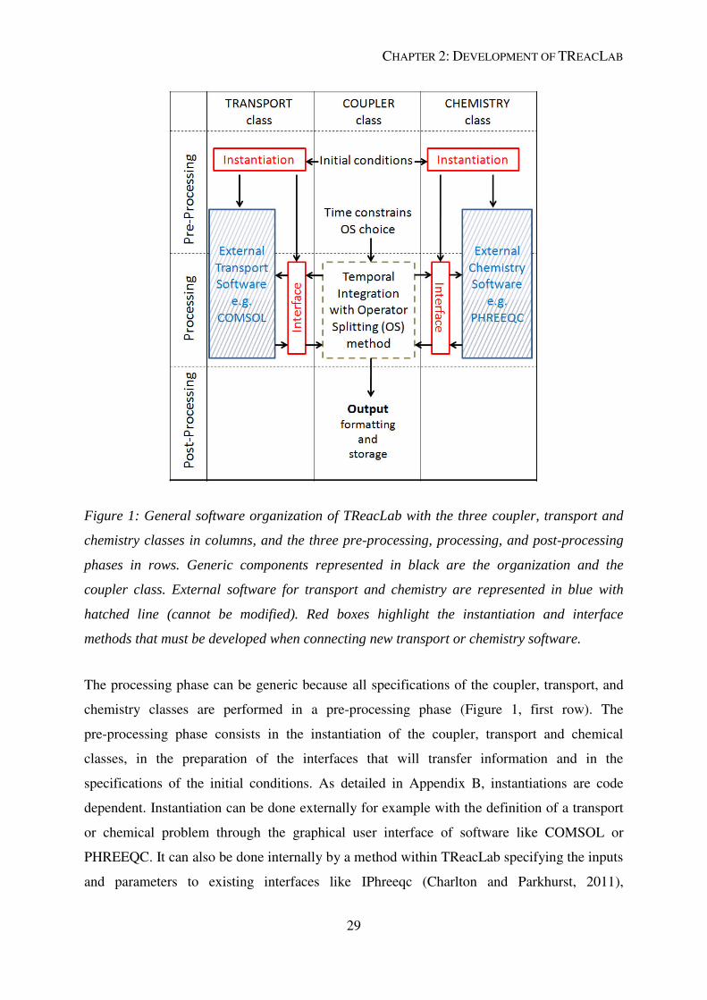
3. Operator splitting implementation and software organization
We provide in TReacLab an object-oriented toolbox for the non-intrusive operator splitting
methods of the previous section. TReacLab is organized along three main components for
coupling transport and reactivity, and proceeds in three pre-processing, processing and
post-processing phases (Figure 1). These three components correspond to the three
well-identified coupler, transport and chemistry classes. The three classes are fully segmented
and exchange information through interfaces. Segmentation ensures that any of the three
coupler, transport and chemistry classes can be replaced without modifications of any of the
two other ones. The solution of the reactive transport problem after spatial discretization
eventually consists in the temporal integration with the chosen OS technique, which
iteratively calls transport and geochemical solvers through interfaces (Figure 1, middle row).
This is the core of the simulation that we identify as the processing phase. It is generic and
does not require at run time any further specification of transport, reactivity and coupler
methods. Standard error management techniques are used to stop the algorithm when any of
the integration method of the three classes fails, stopping the running process and returning
adapted error messages.
CHAPTER 2: DEVELOPMENT OF TREACLAB
29
Figure 1: General software organization of TReacLab with the three coupler, transport and
chemistry classes in columns, and the three pre-processing, processing, and post-processing
phases in rows. Generic components represented in black are the organization and the
coupler class. External software for transport and chemistry are represented in blue with
hatched line (cannot be modified). Red boxes highlight the instantiation and interface
methods that must be developed when connecting new transport or chemistry software.
The processing phase can be generic because all specifications of the coupler, transport, and
chemistry classes are performed in a pre-processing phase (Figure 1, first row). The
pre-processing phase consists in the instantiation of the coupler, transport and chemical
classes, in the preparation of the interfaces that will transfer information and in the
specifications of the initial conditions. As detailed in Appendix B, instantiations are code
dependent. Instantiation can be done externally for example with the definition of a transport
or chemical problem through the graphical user interface of software like COMSOL or
PHREEQC. It can also be done internally by a method within TReacLab specifying the inputs
and parameters to existing interfaces like IPhreeqc (Charlton and Parkhurst, 2011),
CHAPTER 2: DEVELOPMENT OF TREACLAB
30
PhreeqcRM (Parkhurst and Wissmeier, 2015), or COMSOL livelink (COMSOL, 2010). Even
when instantiation is complex, it remains independent for each of the three classes.
Cross-dependencies and feedback between transport and reactivity like density-driven flows
with reacting species are not supported at this stage, although they may be important in some
applications like CO2 sequestration (Abarca et al., 2013).
Pre-processing phase specifies the initial conditions and transfers them to the coupler in
charge of starting the numerical integration. Post-processing is generic and only consists in
formatting and storing output concentrations and solver performances (Figure 1, bottom row).
Specifications are all restricted to the instantiation of the software and interface in the
pre-processing phase while processing and post-processing remain fully generic. Connections
between specific algorithms and generic structures are done by interfaces. Appendix B
provides a detailed description of the transport and chemistry classes, defining the interfaces
to the external codes.
4. Examples and benchmarks
The three following examples validate the methods and illustrate the implementation
presented in sections 2 and 3. The three of them are based on a 1D hydraulically
homogeneous system with steady-state flow and uniform dispersion (equation (2)).The
examples are compared visually against analytical solution or well-know numerical software.
Moreover, we show a convergence study for the first case being the reference solution the
numerical solution with finest time resolution.
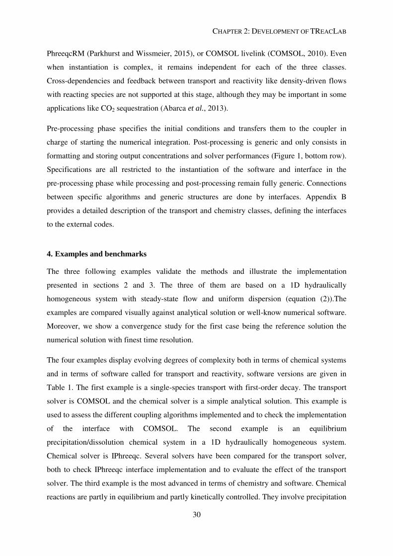
The four examples display evolving degrees of complexity both in terms of chemical systems
and in terms of software called for transport and reactivity, software versions are given in
Table 1. The first example is a single-species transport with first-order decay. The transport
solver is COMSOL and the chemical solver is a simple analytical solution. This example is
used to assess the different coupling algorithms implemented and to check the implementation
of the interface with COMSOL. The second example is an equilibrium
precipitation/dissolution chemical system in a 1D hydraulically homogeneous system.
Chemical solver is IPhreeqc. Several solvers have been compared for the transport solver,
both to check IPhreeqc interface implementation and to evaluate the effect of the transport
solver. The third example is the most advanced in terms of chemistry and software. Chemical
reactions are partly in equilibrium and partly kinetically controlled. They involve precipitation
CHAPTER 2: DEVELOPMENT OF TREACLAB
31
and dissolution reactions. The chemical code is PhreeqcRM. It is used in combination with
COMSOL as transport solver. The last problem face a 2D unsaturated system where transport
is modeled by Richards equation and solved by COMSOL. Chemistry is solved by
PhreeqcRM. These four test cases have been chosen to check the implementation and assess
the coupling methods developed. They are also simple enough from the development point of
view to be taken as starting points to model more advanced chemical systems and transport
conditions.
Software Version
MATLAB R2013b
COMSOL 4.3b
PHREEQC 3.3.7
IPhreeqc 3.3.7
PhreeqcRM 3.3.9
Table 1: Software versions.
4.1. Single-species transport with first-order decay
A single-species transport with first-order decay using different OS methods is compared to
an analytical solution (Van Genuchten and Alves, 1982). The reactive transport system
contains a single solute species of concentration c :
, (18)
where L is given by equation (2). Equation (18) can straightforwardly be separated into
transport and chemistry operators corresponding to the two right-hand side terms.
At time 0, the solute concentration is 0 in the domain (c(x, t=0) = 0). The concentration at the
left boundary is constant and equal to 1 mol/m3
(c(x = 0, t) = 1 mol/m3). The boundary
condition on the right side of the domain is a perfectly absorbing condition (c(x = xmax, t) = 0).
Parameters are derived from Steefel and MacQuarrie (1996) and given in Table 2. The solver
for transport is COMSOL and an analytical solution is used for the first-order decay. Solute
concentration progressively invades the domain from the left boundary with a smooth profile
resulting from the combination of dispersion and decay (Figure 2). Second-order methods
perform much better than first-order methods as expected. Errors are more pronounced at the
CHAPTER 2: DEVELOPMENT OF TREACLAB
32
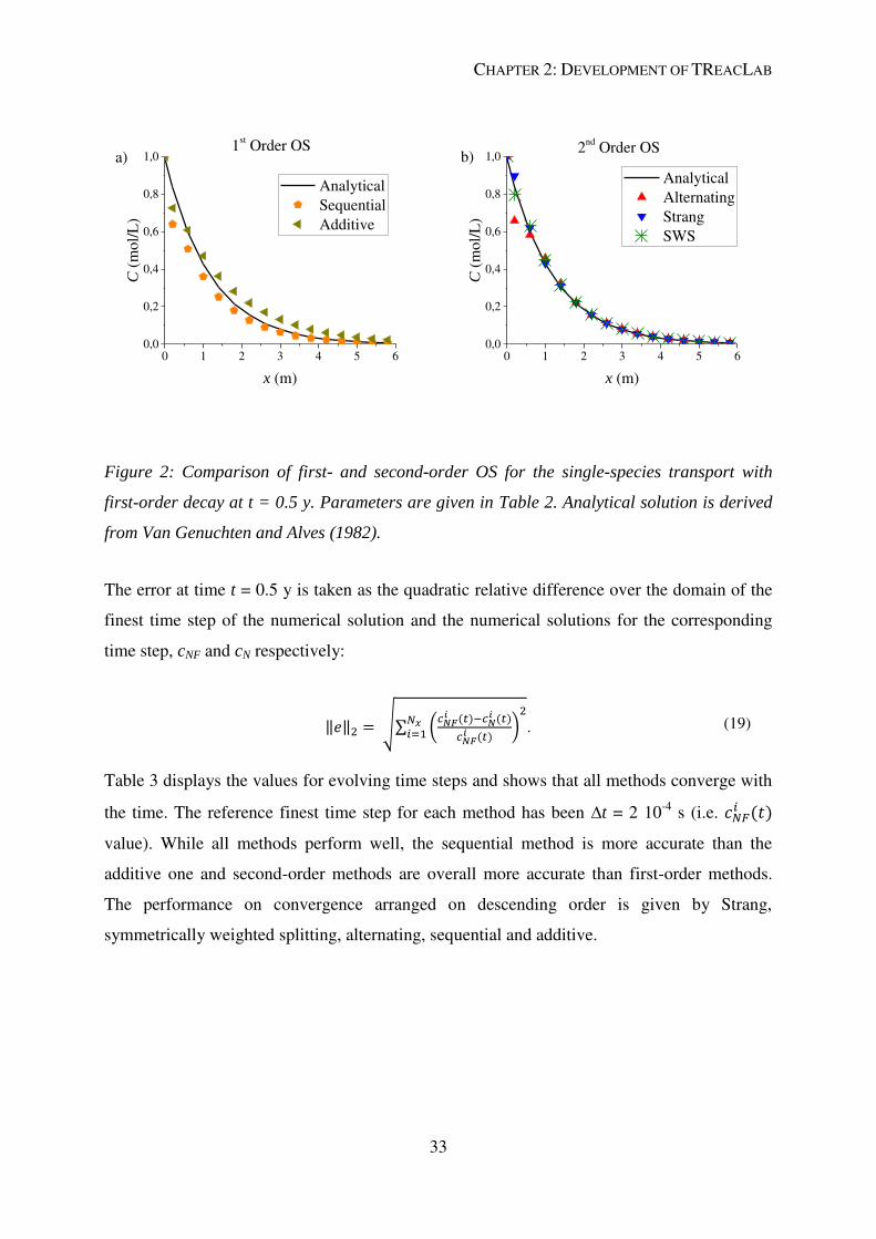
inlet boundary condition on the left side of the domain where the concentration is higher
(Steefel and MacQuarrie, 1996; Valocchi and Malmstead, 1992). The sequential splitting
method with the transport operator performed first overestimates the amount of reaction for
the whole domain since it considers that all incoming solute is getting in without decay for the
full first time step. If the sequence of operators is exchanged, namely first chemistry is solved,
and then transport is solved, the amount of reaction is underestimated. The second-order
alternating splitting, which alternates between transport-chemistry and chemistry-transport
steps, shows strong improvement with compensations between overestimation in the first
application of the chemical operator and underestimation in the second application of the
chemical operator (Simpson and Landman, 2008; Valocchi and Malmstead, 1992).
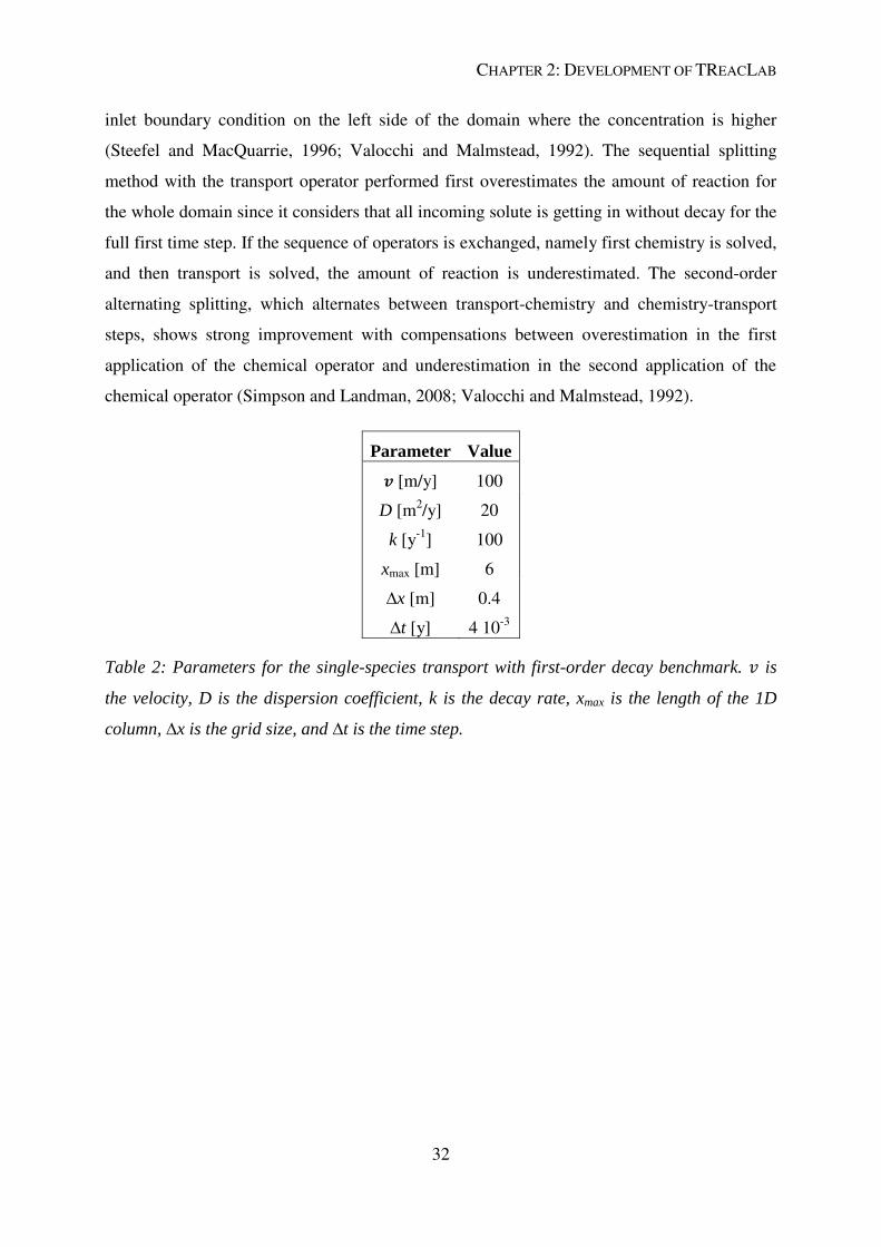
Parameter Value [m/y] 100
D [m2/y] 20
k [y-1
] 100
xmax [m] 6
∆x [m] 0.4
∆t [y] 4 10-3
Table 2: Parameters for the single-species transport with first-order decay benchmark. is
the velocity, D is the dispersion coefficient, k is the decay rate, xmax is the length of the 1D
column, ∆x is the grid size, and ∆t is the time step.
CHAPTER 2: DEVELOPMENT OF TREACLAB
33
0 1 2 3 4 5 60,0
0,2
0,4
0,6
0,8
1,0
C (
mol/
L)
x (m)
Analytical
Sequential
Additive
1st Order OS
a)
0 1 2 3 4 5 60,0
0,2
0,4
0,6
0,8
1,0b)
C (
mol/
L)
x (m)
Analytical
Alternating
Strang
SWS
2nd
Order OS
Figure 2: Comparison of first- and second-order OS for the single-species transport with
first-order decay at t = 0.5 y. Parameters are given in Table 2. Analytical solution is derived
from Van Genuchten and Alves (1982).
The error at time t = 0.5 y is taken as the quadratic relative difference over the domain of the
finest time step of the numerical solution and the numerical solutions for the corresponding
time step, cNF and cN respectively:
. (19)
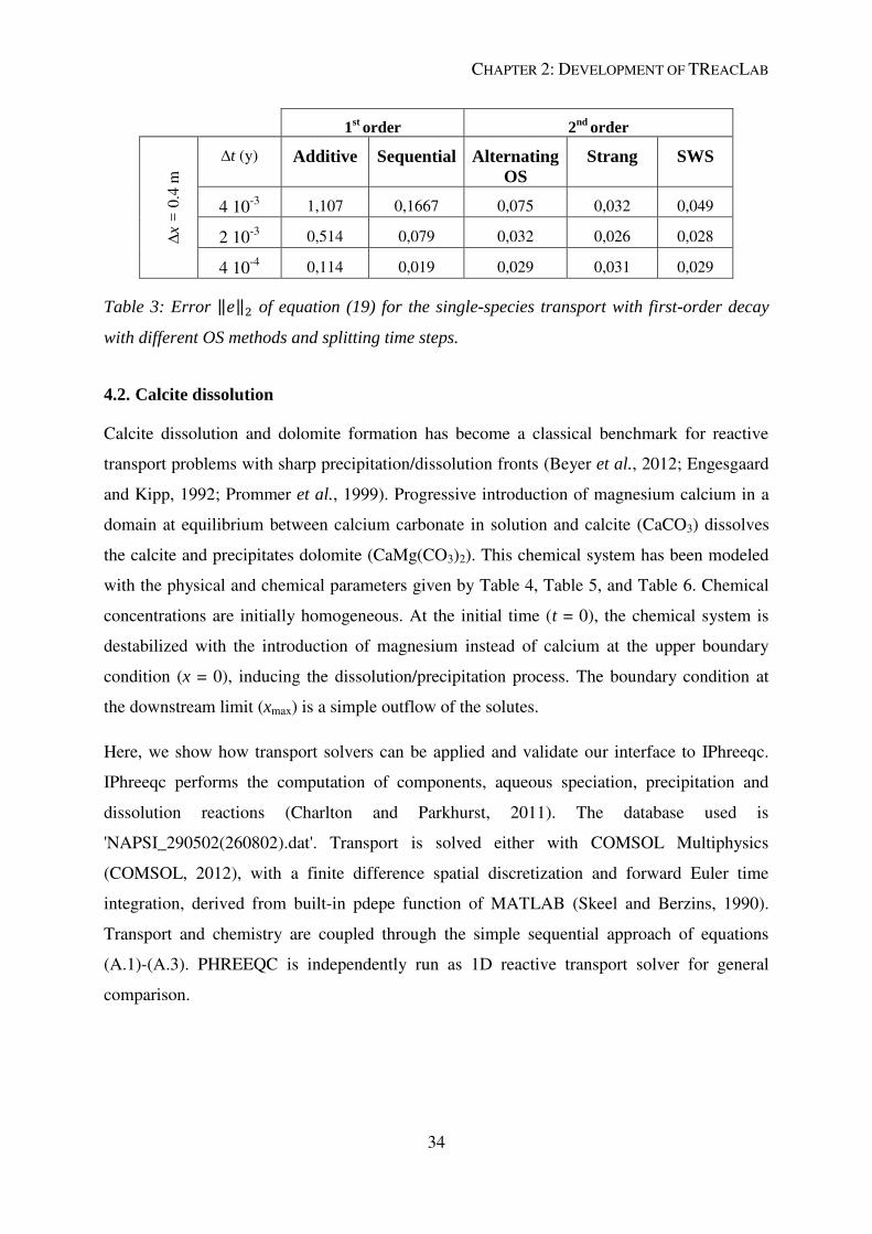
Table 3 displays the values for evolving time steps and shows that all methods converge with
the time. The reference finest time step for each method has been ∆t = 2 10-4
s (i.e. value). While all methods perform well, the sequential method is more accurate than the
additive one and second-order methods are overall more accurate than first-order methods.
The performance on convergence arranged on descending order is given by Strang,
symmetrically weighted splitting, alternating, sequential and additive.
CHAPTER 2: DEVELOPMENT OF TREACLAB
34
1st
order 2nd
order
∆x =
0.4
m
∆t (y) Additive Sequential Alternating
OS
Strang SWS
4 10-3
1,107 0,1667 0,075 0,032 0,049
2 10-3
0,514 0,079 0,032 0,026 0,028
4 10-4
0,114 0,019 0,029 0,031 0,029
Table 3: Error of equation (19) for the single-species transport with first-order decay
with different OS methods and splitting time steps.
4.2. Calcite dissolution
Calcite dissolution and dolomite formation has become a classical benchmark for reactive
transport problems with sharp precipitation/dissolution fronts (Beyer et al., 2012; Engesgaard
and Kipp, 1992; Prommer et al., 1999). Progressive introduction of magnesium calcium in a
domain at equilibrium between calcium carbonate in solution and calcite (CaCO3) dissolves
the calcite and precipitates dolomite (CaMg(CO3)2). This chemical system has been modeled
with the physical and chemical parameters given by Table 4, Table 5, and Table 6. Chemical
concentrations are initially homogeneous. At the initial time (t = 0), the chemical system is
destabilized with the introduction of magnesium instead of calcium at the upper boundary
condition (x = 0), inducing the dissolution/precipitation process. The boundary condition at
the downstream limit (xmax) is a simple outflow of the solutes.
Here, we show how transport solvers can be applied and validate our interface to IPhreeqc.
IPhreeqc performs the computation of components, aqueous speciation, precipitation and
dissolution reactions (Charlton and Parkhurst, 2011). The database used is
'NAPSI_290502(260802).dat'. Transport is solved either with COMSOL Multiphysics
(COMSOL, 2012), with a finite difference spatial discretization and forward Euler time
integration, derived from built-in pdepe function of MATLAB (Skeel and Berzins, 1990).
Transport and chemistry are coupled through the simple sequential approach of equations
(A.1)-(A.3). PHREEQC is independently run as 1D reactive transport solver for general
comparison.
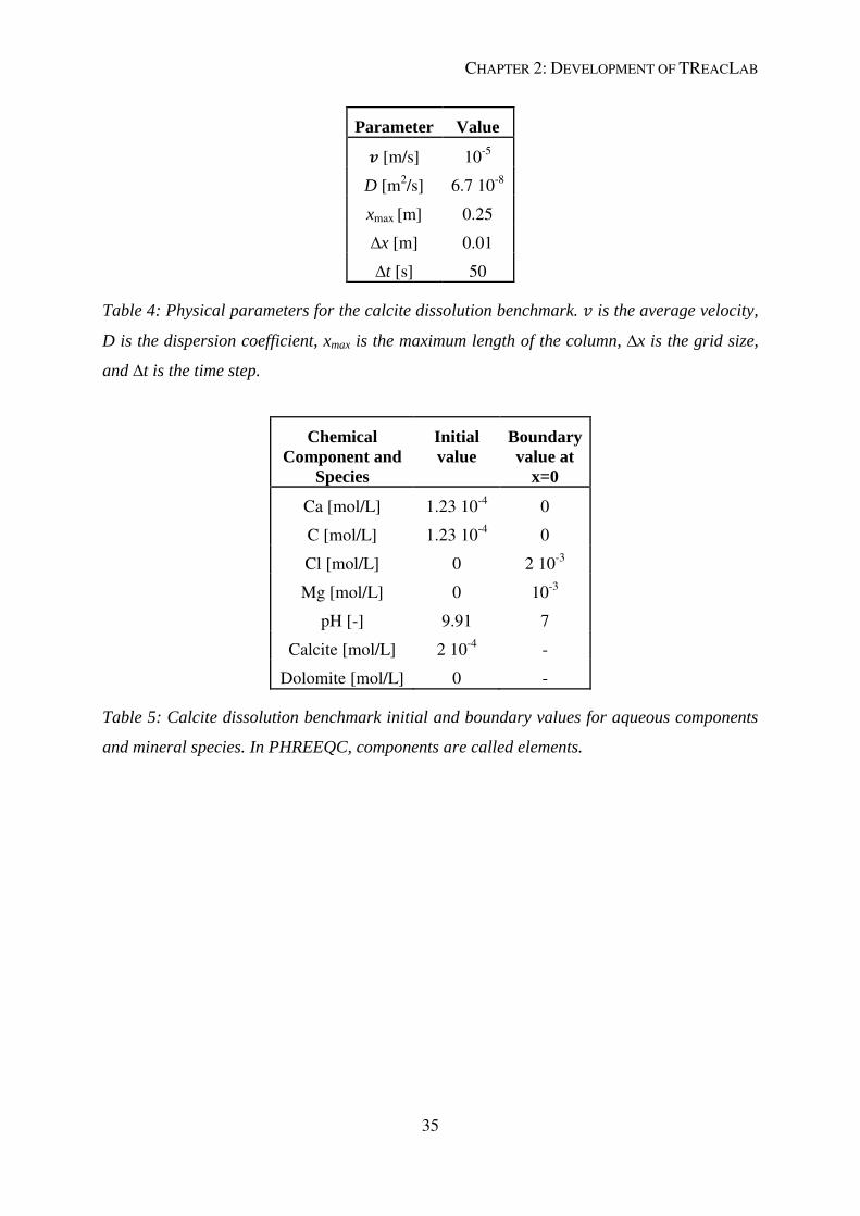
CHAPTER 2: DEVELOPMENT OF TREACLAB
35
Parameter Value [m/s] 10-5
D [m2/s] 6.7 10
-8
xmax [m] 0.25
∆x [m] 0.01
∆t [s] 50
Table 4: Physical parameters for the calcite dissolution benchmark. is the average velocity,
D is the dispersion coefficient, xmax is the maximum length of the column, ∆x is the grid size,
and ∆t is the time step.
Chemical
Component and
Species
Initial
value
Boundary
value at
x=0
Ca [mol/L] 1.23 10-4
0
C [mol/L] 1.23 10-4
0
Cl [mol/L] 0 2 10-3
Mg [mol/L] 0 10-3
pH [-] 9.91 7
Calcite [mol/L] 2 10-4
-
Dolomite [mol/L] 0 -
Table 5: Calcite dissolution benchmark initial and boundary values for aqueous components
and mineral species. In PHREEQC, components are called elements.

CHAPTER 2: DEVELOPMENT OF TREACLAB
36
Homogeneous reactions log (K) -3.1055 -85.9862 27.8493 -13.9995 6.3519 -10.3289 -7.1048 1.1057 -12.78 -7.3492 1.0682 -11.44
Homogeneous reactions
Calcite 1.849
Dolomite 4.118
Table 6: Chemical system of the calcite dissolution benchmark. The upper part comprises the
homogeneous equations and the lower part the heterogeneous reactions. The first column
shows the equilibrium reactions and the second one the logarithms of equilibrium constants.
Figure 3 and Figure 4 display aqueous and mineral equivalent concentrations at time t = 104 s.
As magnesium and chloride get in the domain (Figure 3b and Figure 3d), calcite progressively
dissolves and is replaced by dolomite as expected (Figure 4). Some of the calcium remains in
solution and is flushed out (Figure 3a and Figure 3c). Because of the subsequent absence of
calcium in solution, dolomite dissolves again with some increase of calcium in solution
(Figure 3a and Figure 3c). The three different transport solvers give the same tendency as the
reference PHREEQC solution. COMSOL is closer to the reference value, followed by the
pdepe solver of MATLAB. The better performance of the coupling of IPhreeqc and
COMSOL with respect to the other software couplings is likely coming from the more
accurate time integration scheme of COMSOL for transport in comparison to the other solver.
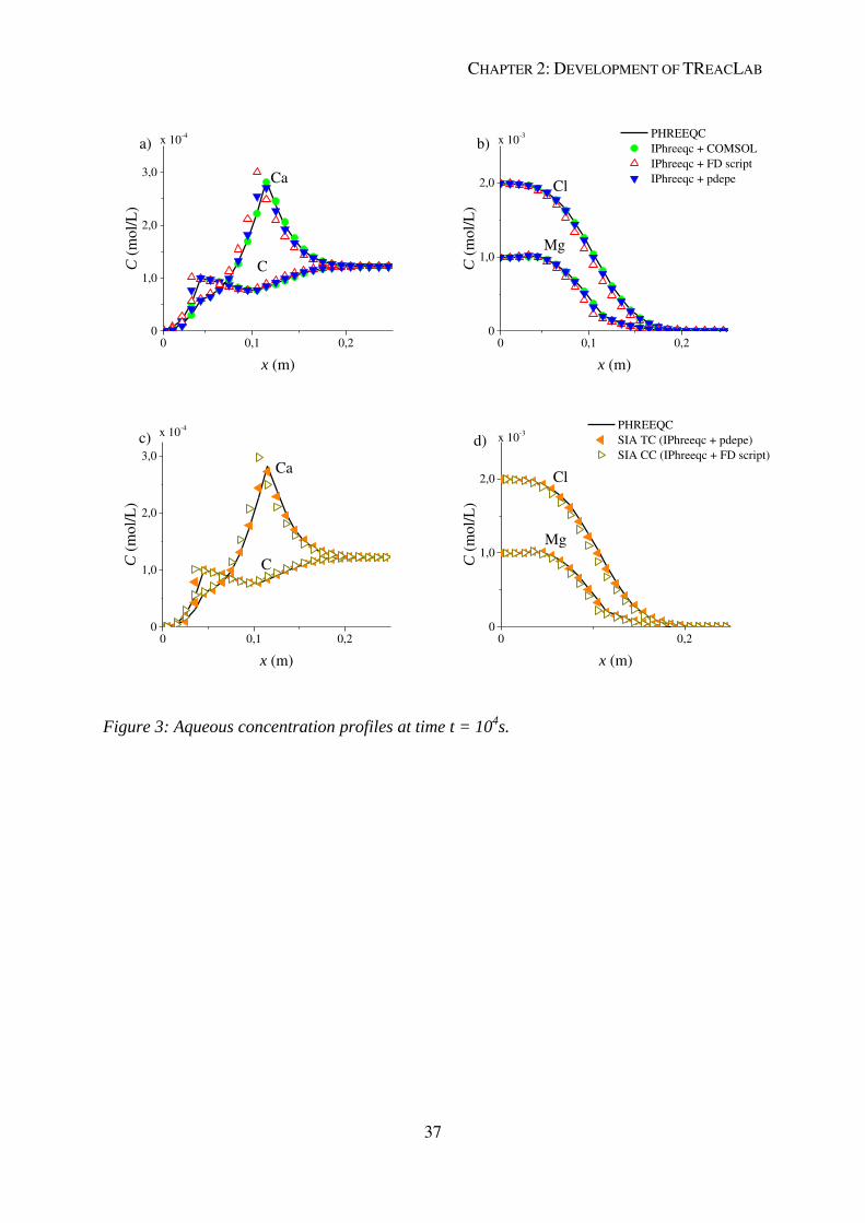
CHAPTER 2: DEVELOPMENT OF TREACLAB
37
0,1 0,20
1,0
2,0
3,0
0
x 10-4
C (
mol/
L)
x (m)
Ca
C
a)
0,1 0,20
1,0
2,0
0
x 10-3 PHREEQC
IPhreeqc + COMSOL
IPhreeqc + FD script
IPhreeqc + pdepe
b)
Mg
C (
mo
l/L
)
x (m)
Cl
0,1 0,20
1,0
2,0
3,0
0
c)
C (
mol/
L)
x (m)
x 10-4
Ca
C
0,20
1,0
2,0
0
PHREEQC
SIA TC (IPhreeqc + pdepe)
SIA CC (IPhreeqc + FD script)d) x 10
-3
C (
mol/
L)
x (m)
Cl
Mg
Figure 3: Aqueous concentration profiles at time t = 104s.

CHAPTER 2: DEVELOPMENT OF TREACLAB
38
0,1 0,20
1,0
2,0
0
PHREEQC
IPhreeqc + COMSOL
IPhreeqc + FD script
IPhreeqc + pdepe
a)
Calcite
C (
mol/
L)
x (m)
Dolomite
x 10-4
Calcite
0,1 0,20
1,0
2,0
0
PHREEQC
SIA TC (IPhreeqc + pdepe)
SIA CC (IPhreeqc + FD script)b)
Dolomite
C (
mol/
L)
x (m)
x 10-4
Figure 4: Dolomite and calcite equivalent concentration profiles with open and filled symbols
respectively at time t = 104
s.
Although COMSOL leads to more accurate results, it is more than one order of magnitude
slower than the two other transport methods (Table 7). We checked that this large difference
in performances does not come from the numerical method but from the large time required
for COMSOL to start and stop when called numerous times externally. While this might not
be an issue for large transport problems for which limitations will rather come from transport
operator, it is a constrain for smaller tests and benchmarks.
Software Coupling Time
IPhreeqc + COMSOL 668 s
IPhreeqc + FD script 24 s
IPhreeqc + pdepe 40 s
Table 7: Time performance for the calcite dissolution benchmark using a sequential operator
splitting.
Whatever the coupling method, the consistency with PHREEQC is overall good. Although
COMSOL uses, as default, implicit time integration schemes for solving the transport
equation instead of the required explicit method, it still compares well with PHREEQC.
Indeed, the sequential non iterative method requires an explicit time integration for transport
CHAPTER 2: DEVELOPMENT OF TREACLAB
39
(equation (13)). It is not the case for COMSOL which uses (as default) a backward
differentiation formula temporal integration scheme, which order varies with the internal time
step adaptation (COMSOL, 2012). It thus introduces an additional error in the coupling
scheme (de Dieuleveult et al., 2009). However, by using such stable and accurate temporal
integrations, it enhances the robustness of the transport scheme.
4.3. Mixed equilibrium-kinetic system
We simulate the progressive increase of dissolved species in an atmospheric water infiltrating
a granitic bedrock. This test case is derived from Nardi et al. (2014). The hydraulic properties
of the system are found in Table 8. The infiltrating water has much lower concentrations of
dissolved species than the resident water. It interacts with five minerals (Table 9). It is in
equilibrium with calcite. The four other minerals k-feldspar, illite, albite and pyrite are subject
to kinetically controlled dissolution with rates ranging from 10-13
to 10-11
mol/s. All
parameters and rate laws of the simulation are provided in the PHREEQC file of iCP (Nardi et
al., 2014). The infiltrating water dissolves calcite to maintain equilibrium, increasing both the
concentration of calcium and the pH of the solution. Other minerals also dissolve and increase
the concentrations of Al and K in solution, however at a much slower rate because of the
kinetic control of the reactions. pH is eventually buffered by the dissolution of illite and
pyrite.
Parameter Value [m/s] 2.78 10-6
m/s
D [m/s] 5.55 10-9
m2/s
xmax [m] 0.08 m
∆x [m] 10-3
m
∆t [s] 720 s
Table 8: Parameters for mixed equilibrium-kinetic benchmark. is the average velocity, D is
the dispersion coefficient, xmax is the maximum length of the column, ∆x is the grid size, and
∆t is the splitting time.
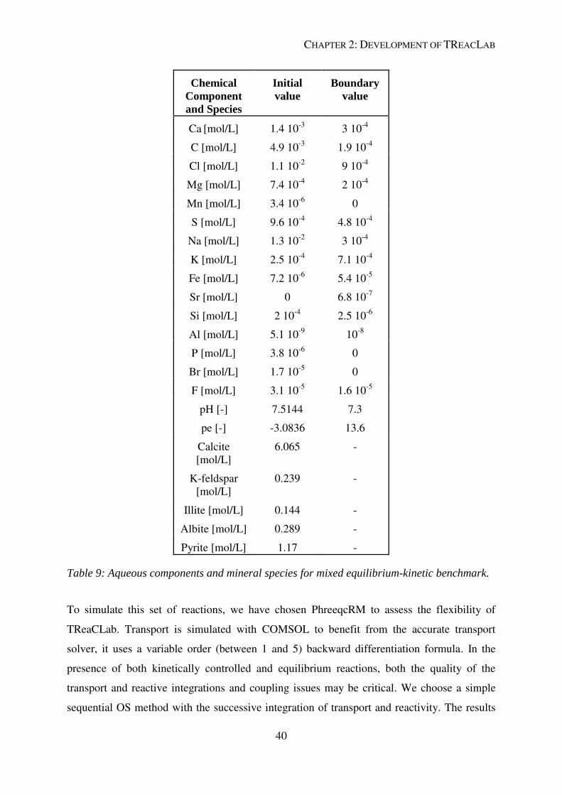
CHAPTER 2: DEVELOPMENT OF TREACLAB
40
Chemical
Component
and Species
Initial
value
Boundary
value
Ca [mol/L] 1.4 10
-3 3 10
-4
C [mol/L] 4.9 10-3
1.9 10-4
Cl [mol/L] 1.1 10-2
9 10-4
Mg [mol/L] 7.4 10-4
2 10-4
Mn [mol/L] 3.4 10-6
0
S [mol/L] 9.6 10-4
4.8 10-4
Na [mol/L] 1.3 10-2
3 10-4
K [mol/L] 2.5 10-4
7.1 10-4
Fe [mol/L] 7.2 10-6
5.4 10-5
Sr [mol/L] 0 6.8 10-7
Si [mol/L] 2 10-4
2.5 10-6
Al [mol/L] 5.1 10-9
10-8
P [mol/L] 3.8 10-6
0
Br [mol/L] 1.7 10-5
0
F [mol/L] 3.1 10-5
1.6 10-5
pH [-] 7.5144 7.3
pe [-] -3.0836 13.6
Calcite
[mol/L]
6.065 -
K-feldspar
[mol/L]
0.239 -
Illite [mol/L] 0.144 -
Albite [mol/L] 0.289 -
Pyrite [mol/L] 1.17 -
Table 9: Aqueous components and mineral species for mixed equilibrium-kinetic benchmark.
To simulate this set of reactions, we have chosen PhreeqcRM to assess the flexibility of
TReaCLab. Transport is simulated with COMSOL to benefit from the accurate transport
solver, it uses a variable order (between 1 and 5) backward differentiation formula. In the
presence of both kinetically controlled and equilibrium reactions, both the quality of the
transport and reactive integrations and coupling issues may be critical. We choose a simple
sequential OS method with the successive integration of transport and reactivity. The results
CHAPTER 2: DEVELOPMENT OF TREACLAB
41
obtained by the coupling of COMSOL and PhreeqcRM are close to the reference solution
given by PHREEQC alone for the dissolved species and kinetically dissolving minerals
(Figure 5). The time step of the coupled PhreeqcRM and COMSOL integration has been taken
smaller than the characteristic mesh scale transport time and reactive time at least for the
kinetical reaction to ensure accurate integrations. The most difficult quantity to get accurately
is the calcium concentration because calcite is at equilibrium. The time step must be reduced
to recover a steeper reactive front (Figure 6).
This more advanced test shows that the computational load should be well balanced between
the coupler, transport and chemistry methods. While coupling is the critical component in
cases of equilibrium reactions and may even require highly integrated coupling strategies like
global implicit methods (Hoffmann et al., 2010; Saaltink et al., 2001), it is not the case for
kinetically controlled reactions. In this case of mixed equilibrium kinetic reaction, elementary
coupling and accurate transport and reactive solvers can be efficient with small enough time
steps where sharp reaction fronts are involved.

CHAPTER 2: DEVELOPMENT OF TREACLAB
42
50 10
4
0
8
x 104
Al
(mol/
L)
t (s)
PHREEQC
PhreeqcRM + COMSOLx 10
-8
a)
50 10
2
8
-4
14b)
x 104
pe
t (s)
0 5 102
4
6
8c)x 10
-4
x 104
K (
mo
l/L
)
t (s)
50 10
8,4
7,4
9,2d)
x 104
pH
t (s)
Figure 5: Comparison of results between the coupling of PhreeqcRM and COMSOL and
PHREEQC observed for the mixed equilibrium-kinetic benchmark at the output of the column.

CHAPTER 2: DEVELOPMENT OF TREACLAB
43
0 7 14 210
4
8
12
16
x10-3
x10-3
Dis
solv
ed c
alci
te (
mol)
x (m)
PHREEQC (Reference)
PhreeqcRM + COMSOL t = 720 s
PhreeqcRM + COMSOL t = 360 s
PhreeqcRM + COMSOL t = 90 s
Figure 6: Quantity of dissolved calcite with PhreeqcRM and COMSOL for two different
splitting time steps ∆t = 720 s, 360 s and 90 s. PHREEQC independently is used as reference.
4.4. Pesticide infiltration
The following benchmark concerns the infiltration in an unsaturated soil column of a
carbamate insecticide (Aldicarb) (MIKE(DHI), 2016; Multiphysics, 2008; Šimůnek et al.,
1994; Wissmeier and Barry, 2011). The soil column is a 2D cylinder made up of two layers
with a smaller hydraulic conductivity in the upper layer but higher saturation. Transport is
modeled by Richards' equation and solved by COMSOL (Figure 7). Aldicarb is transported
downwards and sideways from the infiltration (top of the column from r = 0 m to r = 0.25 m).
Chemistry is described by first-order decay chain reactions (Figure 8), being only mobile
Aldicarb, Aldicarb sulfoxide and Aldicarb sulfone (i.e. the other species are fix species).
These system of ordinary differential equations is solved by PhreeqcRM.
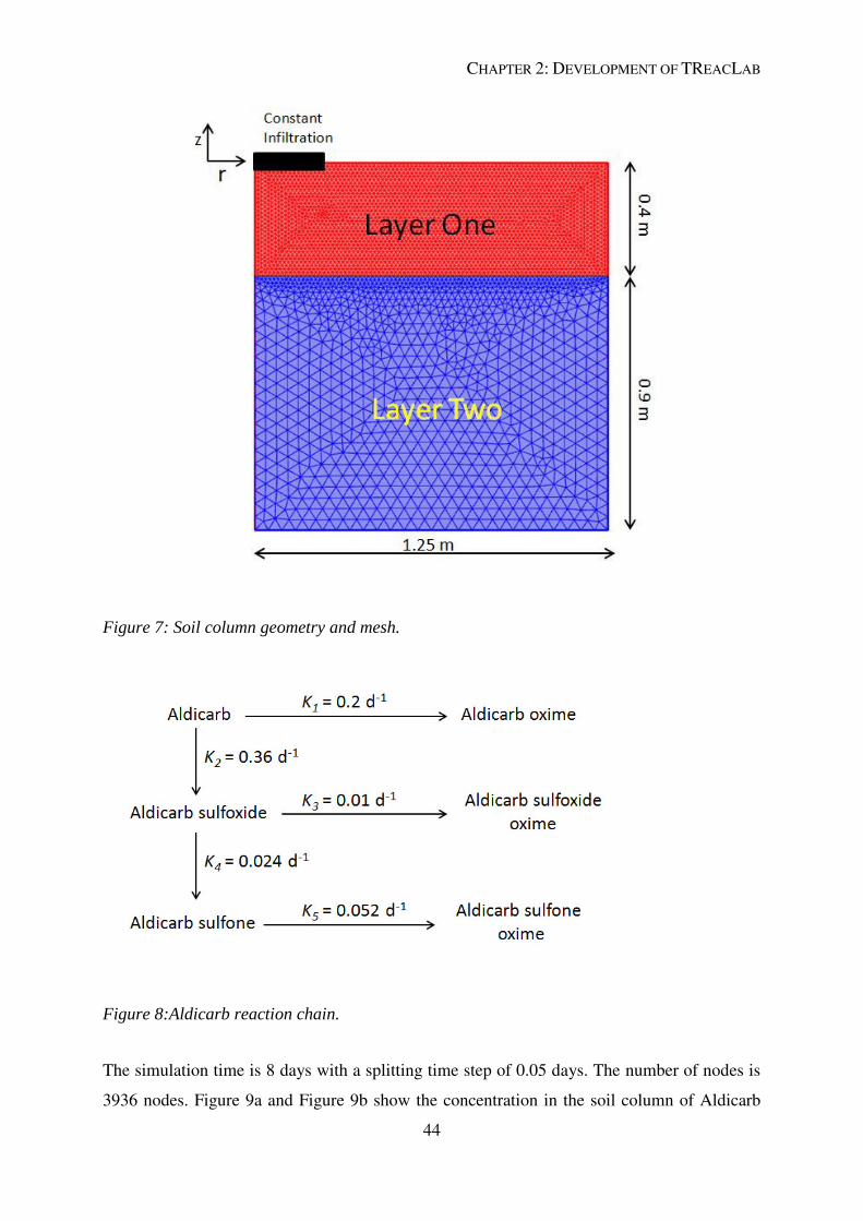
CHAPTER 2: DEVELOPMENT OF TREACLAB
44
Figure 7: Soil column geometry and mesh.
Figure 8:Aldicarb reaction chain.
The simulation time is 8 days with a splitting time step of 0.05 days. The number of nodes is
3936 nodes. Figure 9a and Figure 9b show the concentration in the soil column of Aldicarb
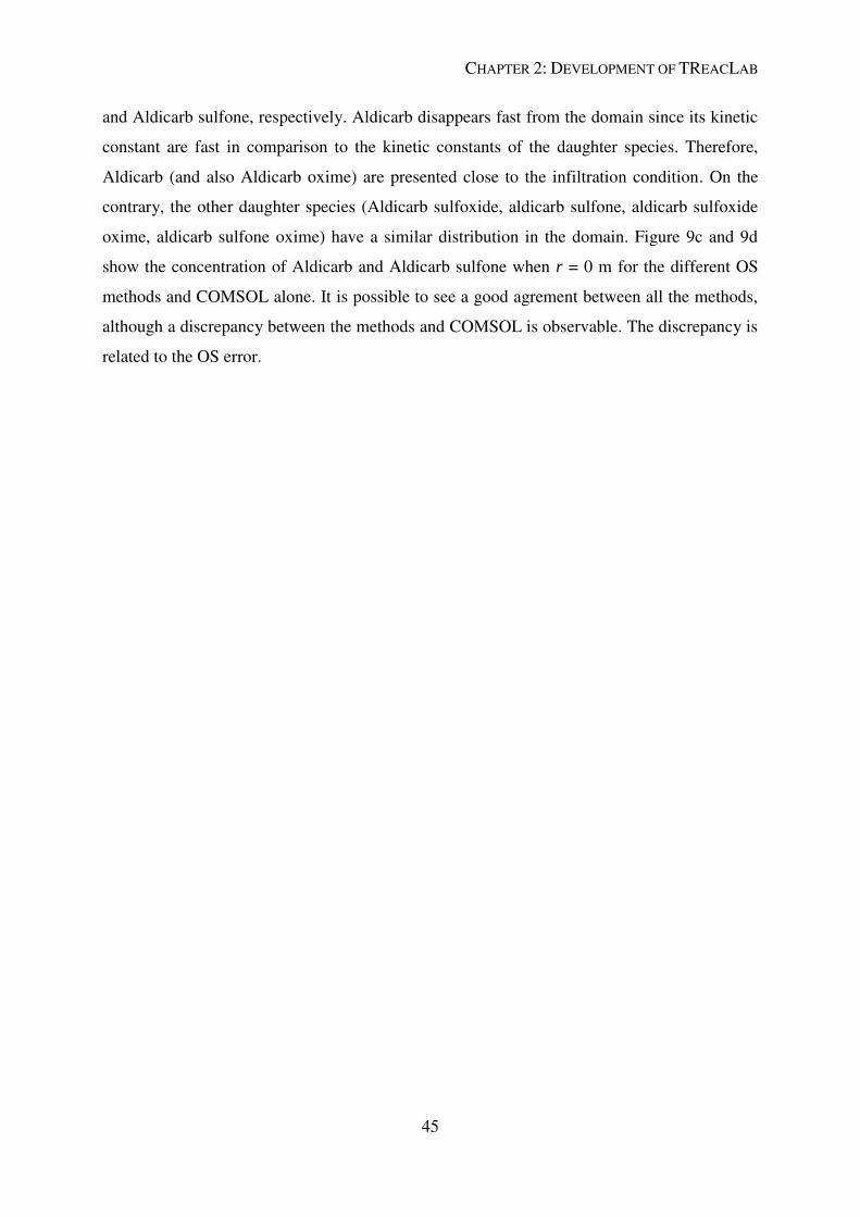
CHAPTER 2: DEVELOPMENT OF TREACLAB
45
and Aldicarb sulfone, respectively. Aldicarb disappears fast from the domain since its kinetic
constant are fast in comparison to the kinetic constants of the daughter species. Therefore,
Aldicarb (and also Aldicarb oxime) are presented close to the infiltration condition. On the
contrary, the other daughter species (Aldicarb sulfoxide, aldicarb sulfone, aldicarb sulfoxide
oxime, aldicarb sulfone oxime) have a similar distribution in the domain. Figure 9c and 9d
show the concentration of Aldicarb and Aldicarb sulfone when r = 0 m for the different OS
methods and COMSOL alone. It is possible to see a good agrement between all the methods,
although a discrepancy between the methods and COMSOL is observable. The discrepancy is
related to the OS error.
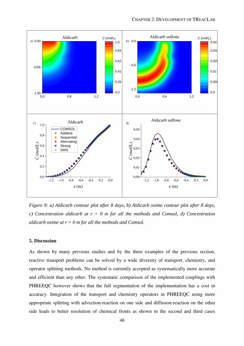
CHAPTER 2: DEVELOPMENT OF TREACLAB
46
0,0 0,6 1,2-1,30
-0,65
0,00
0,0
0,20
0,41
0,62
0,83
1,0
C (mol/L)a)
Aldicarb
0,0 0,6 1,2
-1,2
-0,6
0,0b)
Aldicarb sulfone
0,0
0,0081
0,017
0,025
0,034
0,041
C (mol/L)
-1,2 -1,0 -0,8 -0,6 -0,4 -0,2 0,00,0
0,2
0,4
0,6
0,8
1,0
C (
mo
l/L
)
z (m)
COMSOL
Additive
Sequential
Alternating
Strang
SWS
Aldicarbc)
-1,2 -1,0 -0,8 -0,6 -0,4 -0,2 0,00,00
0,01
0,02
0,03
0,04
0,05
Aldicarb sulfone
C (
mo
l/L
)
z (m)
d)
Figure 9: a) Aldicarb contour plot after 8 days, b) Aldicarb oxime contour plot after 8 days,
c) Concentration aldicarb at r = 0 m for all the methods and Comsol, d) Concentration
aldicarb oxime at r = 0 m for all the methods and Comsol.
5. Discussion
As shown by many previous studies and by the three examples of the previous section,
reactive transport problems can be solved by a wide diversity of transport, chemistry, and
operator splitting methods. No method is currently accepted as systematically more accurate
and efficient than any other. The systematic comparison of the implemented couplings with
PHREEQC however shows that the full segmentation of the implementation has a cost in
accuracy. Integration of the transport and chemistry operators in PHREEQC using more
appropriate splitting with advection-reaction on one side and diffusion-reaction on the other
side leads to better resolution of chemical fronts as shown in the second and third cases
CHAPTER 2: DEVELOPMENT OF TREACLAB
47
(Parkhurst and Appelo, 1999). It is not only the integration but also the successive
improvements of the methods that lead to significantly more accurate schemes. While results
are less accurate with TReacLab, they remain however close displaying the same overall
behavior both on solute and mineral concentrations. The interest of fully segmented reactive
transport implementations like in TReacLab is not motivated by the accuracy and should not
be used when other more integrated and optimized software are appropriate and freely
available.
Despite their lower accuracy, fully segmented implementations may be useful in situations
where flexibility is essential. It is the case when extensive modeling work has been performed
in independent software environments for transport or chemistry, and extensions to reactive
transport problems are required. Transport and chemistry solvers are then imposed and should
be coupled with as few specific developments as possible. For example, COMSOL and
PHREEQC have been interfaced here and in several other works because of their
complementarity (Nardi et al., 2014; Nasir et al., 2014; Wissmeier and Barry, 2011). It is
possible to specify advanced geometrical configurations in COMSOL through a convenient
graphical user interface (Azad et al., 2016). PHREEQC provides advanced capacities for
modeling complex geochemical systems with extensive database of reactions (Charlton and
Parkhurst, 2011; Parkhurst and Wissmeier, 2015). In such cases, building the structure of the
model may be the first and dominant issue in developing simulation capacities. That is when
codes like TReacLab can provide practical bridges for reactive transport systems. The
examples of section 4 however shows that they must be used with great care. Especially, the
called software may have different temporal integration schemes than the explicit and implicit
methods required by the SNIA and SIA coupling methods as discussed for the higher-order
schemes of COMSOL in section 0. Using codes like COMSOL may enhance robustness at a
certain cost of accuracy. Thus, implementation capacity does not guarantee validity. Validity
must be carefully checked and argued with other comparable cases or with appropriate
convergence analysis.
Another targeted use of TReacLab concerns the development and test of new coupling
methods or strategies. Operator splitting can be performed with various methods including for
example adaptative time stepping (Belfort et al., 2007; Gasda et al., 2011). Global implicit
approaches that separate geochemical and transport software might also be more widely tested
providing the Jacobian of the chemical operator and taking into account current limitations
CHAPTER 2: DEVELOPMENT OF TREACLAB
48
such as the difficulties to model precipitation/dissolution reactions (Amir and Kern, 2010).
TReacLab may then be used as a platform where interfaces to chemical and transport
operators are available and have been tested and documented for other coupling methods.
These applications are possible because TReacLab is a fully free and open software that can
be directly accessed and downloaded (https://github.com/TReacLab/TReacLab). The free and
open use of TReacLab has been dominant in its development and in the choices made for its
organization. The repository thus provides two main directories with sources and examples
respectively. Sources are organized in four main categories for chemistry, transport, coupler
and utilitaries. At the root of the chemistry, transport and coupler directories are the virtual
classes as main entries. Examples of instantiations are provided in the subdirectories.
Additional developments may take advantage of the documented examples provided at the
different levels of the software.
6. Conclusion
We provide in the TReacLab code a fully segmented implementation of the coupling of
independent geochemical and transport software. Coupling is based on a general expression of
the split-operator strategy with a set of classical methods. TReacLab should facilitate the
development of reactive transport simulation capacities for independent reactive and transport
software. Systematic comparison to the well-established PHREEQC model for uniform 1D
reactive transport cases shows that full decoupling at the implementation level has a cost in
accuracy. Sharp dissolution fronts of thermodynamically controlled reactions especially are
generally smoothed. Steeper fronts might be recovered with smaller splitting time steps at
larger computational costs. Beyond the implementation and the simulation capacity,
consistency and validity of the numerical models should be systematically assessed.
TReacLab can be freely accessed and used to promote the development of coupling methods
and to provide additional modeling capacity for reactive transport coupling in geological
media.
Appendix A: Implemented operator splitting methods
We detail the mathematical formulation for the sequential splitting (Geiser, 2009) :
, , , (A.1)
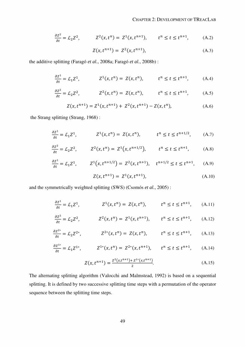
CHAPTER 2: DEVELOPMENT OF TREACLAB
49
, , , (A.2)
, (A.3)
the additive splitting (Faragó et al., 2008a; Faragó et al., 2008b) :
, , , (A.4)
, , , (A.5)
, (A.6)
the Strang splitting (Strang, 1968) :
, , , (A.7)
, , , (A.8)
, , , (A.9)
, (A.10)
and the symmetrically weighted splitting (SWS) (Csomós et al., 2005) :
, , , (A.11)
, , , (A.12)
, , , (A.13)
, , , (A.14)
. (A.15)
The alternating splitting algorithm (Valocchi and Malmstead, 1992) is based on a sequential
splitting. It is defined by two successive splitting time steps with a permutation of the operator
sequence between the splitting time steps.
CHAPTER 2: DEVELOPMENT OF TREACLAB
50
Appendix B: Complementary notes on software organization
We successively describe the general toolbox organization, the coupler, transport and
chemistry classes. We concretely show how operator splitting methods can be introduced and
how other transport and geochemical codes can be connected.
B.1 Coupling methods
The coupler is at the center of TReacLab as it performs the temporal integration and calls the
transport and chemistry solvers through the OS algorithm. In the pre-processing phase, it gets
the initial conditions and the temporal constrains of the integration. It is also in charge of
storing the required results before formatting and outputting them in the post-processing
phase. Because the coupler is at the core of the toolbox, its methods remain generic.
Interactions with the transport and chemistry solvers are also fully generic thanks to template
interfaces calling external software and managing the exchange of information. Calling
external software relies on the so-called Solve_Engine method for both transport and
chemistry software. Solve_Engine takes as inputs the concentration data and the time step
over which the integration must be performed. It returns the updated concentrations, a flag to
check the success of the integration and an error message in case of failure to activate and
inform the error management procedure mentioned in the former section. The coupler is based
on a fixed structure of concentration data. Whatever the structure of concentrations in the
transport and chemical codes, the structure of concentrations within the coupler is always the
same. It consists in a matrix with in columns chemical species and in rows the position within
the domain (Figure B.1). The size of the matrix is equal to the number of cells times the
number of chemical species and components passed through the coupler. Chemical species
include solutes and fixed species. As this is the sole link between the chemical code and the
coupler also in charge of temporary results storage for the post-processing, it must transfer all
quantities necessary for the algorithm and for the later extraction. The format of the matrix is
set in the pre-processing phase and it is fixed for the whole simulation. TReacLab does not
support yet any modification of species number to transfer between codes. Even if some
solute species are absent over some time of the simulation, they will be transferred. This
choice does not limit the capacity of the software as long as the chemical system is known
from the beginning but might have some consequences on its performance in cases where
solute composition strongly evolves. The choice of generality and flexibility, here like in
other places, has a cost in efficiency. All modifications of concentration format are eventually
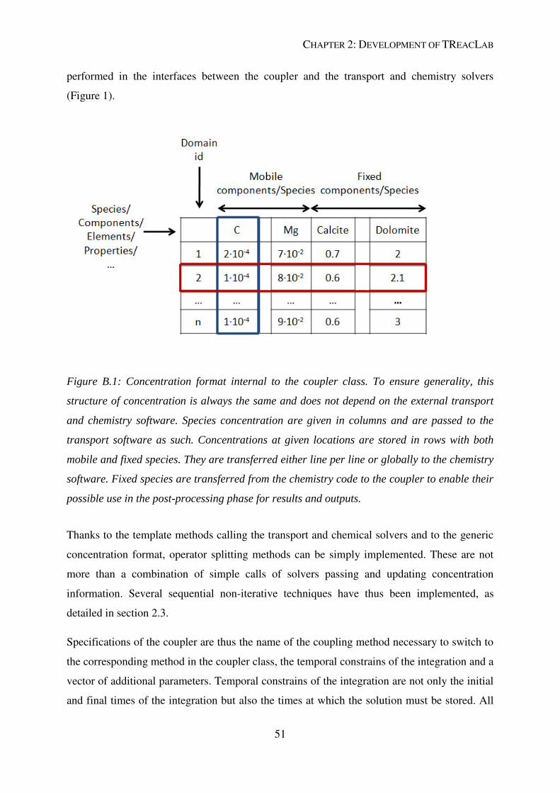
CHAPTER 2: DEVELOPMENT OF TREACLAB
51
performed in the interfaces between the coupler and the transport and chemistry solvers
(Figure 1).
Figure B.1: Concentration format internal to the coupler class. To ensure generality, this
structure of concentration is always the same and does not depend on the external transport
and chemistry software. Species concentration are given in columns and are passed to the
transport software as such. Concentrations at given locations are stored in rows with both
mobile and fixed species. They are transferred either line per line or globally to the chemistry
software. Fixed species are transferred from the chemistry code to the coupler to enable their
possible use in the post-processing phase for results and outputs.
Thanks to the template methods calling the transport and chemical solvers and to the generic
concentration format, operator splitting methods can be simply implemented. These are not
more than a combination of simple calls of solvers passing and updating concentration
information. Several sequential non-iterative techniques have thus been implemented, as
detailed in section 2.3.
Specifications of the coupler are thus the name of the coupling method necessary to switch to
the corresponding method in the coupler class, the temporal constrains of the integration and a
vector of additional parameters. Temporal constrains of the integration are not only the initial
and final times of the integration but also the times at which the solution must be stored. All
CHAPTER 2: DEVELOPMENT OF TREACLAB
52
time related parameters are stored into a time class. Additional parameters may be tolerances
for example when using sequential iterative approaches. Instantiation of the coupler class thus
consists in providing the identifier of the chosen coupling technique, the time constrains in the
time class (initial time, final time, time to save the results, OS time step) and the additional
parameters possibly needed by the algorithm.
B.2 Geochemical solver
Geochemical codes widely differ by their principles, the type of reactivity they consider and
their input/output formats and parameters. We propose to normalize some of their interface to
simplify exchanges with the coupler. In any case of equilibrium or kinetic reactions or of a
mixed combination of them, geochemical codes steadily take concentrations, reaction
constants, rate parameters, reaction times, as inputs and return output concentrations. All
specifications linked to the choice of components, primary and secondary species should be
set in the geochemical code or in the interface so that the geochemical solver does not have to
be modified and the coupler remains generic. Whether components are used or not, the
definition of the chemical system is not unique. Even when components are used, several
alternative and reliable definitions can be chosen (Fang et al., 2003; Hoffmann et al., 2012;
Molins et al., 2004). Numerical and conceptual consistencies between the transport and
chemical systems should thus be ensured externally before any implementation.
While solute concentrations are instantiated by the coupler and systematically passed to the
geochemical solver, equilibrium and kinetic constants are considered as constant. They are
defined once for all in the pre-processing phase. For example in PHREEQC, chemical
reactions and constants are already defined in databases like 'Phreeqc.dat' or 'llnl.dat'.
Initialization of mineral quantities is done at the beginning of the simulation when setting the
initial conditions through the coupler. The interface between the coupler and the geochemical
solver is made up of the Solve_Engine that calls the geochemical solver and the methods that
modify the concentration format. By default, the geochemical solver is instantiated and stored
for each of the nodes of the computational grid for the whole domain of the simulation. Any
data that are not passed to the coupler is, in general, kept in the instances of the geochemical
code. Another option is provided by software that allow simultaneous computations for
several independent batches like it is for example the case of PHREEQC. In such cases only
one instance of the geochemical solver is necessary. Exchanges of data between the coupler
and the geochemical solver are defined in the pre-processing phase and remain fixed for the
CHAPTER 2: DEVELOPMENT OF TREACLAB
53
whole duration of the simulation. It is precisely at this stage that components are derived
through the algebraic operations of equation (6) and passed to the coupler. The coupler does
not manage the transformation of concentration and species but just their transfer between the
transport and geochemical solvers. The use of components does not fundamentally change the
calling sequence of the geochemical operator but modifies its interface to the coupler.
Components may be specified by the geochemical code like in PHREEQC or by the user in
the pre-processing phase by loading the matrix of U (equation (6)). In this latter case,
components are defined by the user in the pre-processing phase and are computed by the
interface that adapts the information to be passed through the coupler to the transport solver.
Connection of a new geochemical code requires essentially four operations. First, a new
daughter class of the template chemistry class must be defined. It can be built up using, as
template, one of the examples provided and described in the section 4. Second, an interface
must be created to filter the required information given from the coupler to the Solve_Engine
method. Third, an instantiation procedure should be provided whether it is internal or external
to TReacLab. Fourth, the template Solve_Engine calling function of the geochemical solver
must be written and optionally tested before being effectively used in reactive transport
problems.
B.3 Transport solver
Despite the diversity of the transport mechanisms and numerical schemes to solve them, we
provide here a basic interface designed mostly to address transport in a generic way. As
previously stated, this approach assumes that transport parameters are not modified by the
species concentration. This absence of feedback currently precludes density driven flows as
well as permeability and porosity modifications due to precipitation or dissolution. TReacLab
might be extended in this direction on the basis of slow evolutions of porosity or density. The
transport operator relies on concentration independent parameters. We detail in the following
the interaction between the coupler and the transport classes with the exchange of data and the
instantiation of the transport solver. We will conclude this section with the development
required to connect other transport codes.
While geochemical codes operate on species concentration on a given computational node,
transport codes operate on a given species concentration over all the domain. In terms of data
structure, each of the columns of the concentration array are successively transferred to the
CHAPTER 2: DEVELOPMENT OF TREACLAB
54
geochemical code and each of the rows (or linear combinations of rows) are given to the
transport code (Figure B.1). The transport operator is thus iteratively called for each of the
species or components explicitly specified in the interface between the coupler and the
transport solver (Figure 1). The time range over which temporal integration should be
performed and the identifiers of the transported species are also transferred to the transport
solver. Species identification is essential when considering species sensitive diffusion
coefficient. The transport solver returns the updated concentration field at the final time of the
time range, an indicator of success or failure of the integration and a message to document
algorithm failures. The basic exchange of concentrations with the imposed integration times
are the sole requirements for the coupler to proceed.
All other parameters of the transport code should be set in the pre-processing phase, which
may become an important part of the eventual reactive transport code. In fact it does not cover
only the flow and transport parameters but more broadly the full structure of the domain, of
the computational grid, and of the boundary conditions. As for the geochemical code, the
transport code can be instantiated internally or externally. In case of internal definition, it
should contain at least the flow and transport properties, the morphology of the domain and
the structure of the computational grid (coordinates of the computational nodes). A default set
of classes is provided for 1D problems as templates for the morphology (domain definitions),
the computational grid (identification and coordinates of nodes and edges), the boundary
conditions (nature and values for boundary conditions) and the hydraulic and transport
properties. We recall as also said in section 2.2 that some operator splitting techniques might
impose limitations on the transport solver in terms of integration scheme or in terms of time
step (de Dieuleveult et al., 2009). Both the OS technique and the transport integration should
be chosen consistent.
Operations on the transport class are thus decomposed between the pre-processing and the
processing phases. Specifications of the operator with all necessary parameters is performed
in the pre-processing phase. Only generic exchanges of concentrations are needed in the
processing phase. Additional information would generally be needed externally to identify the
location of the computational nodes. More advanced information from the definition of the
domain, parameters and boundary conditions will be generally defined in the transport code
rather than in TReacLab. For example, Comsol or Modflow have their own grid definitions.
They are complete and efficient. It may be straightforwardly extracted and cross-referenced
CHAPTER 2: DEVELOPMENT OF TREACLAB
55
with the results of TReacLab as long as the cell numbers correspond, a basic but necessary
requirement. This choice is motivated by both the generality and the simplicity of TReacLab.
It also highlights that TReacLab remains a coupler that transfers information and does not
process in any way the relation of concentrations between cells like a transport operator does.
The methodological choice of handling the spatial dimension of the problem within the
transport operator is not only operational. It is also ensuring the capacity to connect a wide
range of transport codes with their own logic and structure. For example, the multi-physics
software COMSOL has its own mesh generator methods and internal structures that should
not be duplicated in TReacLab but interfaced. Connecting other codes would thus require
reduced work as long as they can already be called from the same environment of
development (here MATLAB) on a discretized time basis. More in details, any new transport
code would require: 1) the development of the main calling function Solve_Engine to call it
from the coupler 2) the adaptation of the concentration format in the interface methods that
match the concentrations to the internal data structure of the external code, 3) the instantiation
of the transport class and 4) the access to the coordinates of the computational nodes for
outputs purposes. As for the geochemical code, implementation of the interface should be
checked before any full reactive transport coupling. This can be completed within TReacLab
by using an idle process instead of the geochemical code.
Acknowledgements: We acknowledge ANDRA and the ANR project H2MNO4 under the
number ANR-12-MONU0012-01 for their financial support, Jocelyne Erhel and David L.
Parkhurst for constant and fruitful discussions, and Javier Molinero for initial exchanges.
CHAPTER 2: DEVELOPMENT OF TREACLAB
56
REFERENCES
Abarca, E., Nardi, A., Grandia, F., Molinero, J., 2013. Feedback between reactive transport
and convective flow during CO2 migration in a saline aquifer, EGU General
Assembly Conference Abstracts, p. 7707.
Amir, L., Kern, M., 2010. A global method for coupling transport with chemistry in
heterogeneous porous media. Computational Geosciences 14, 465-481.
Apoung-Kamga, J.-B., Have, P., Houot, J., Kern, M., Semin, A., 2009. Reactive Transport in
Porous Media. ESAIM: Proceedings 28, 227 - 245.
Azad, V.J., Li, C., Verba, C., Ideker, J.H., Isgor, O.B., 2016. A COMSOL–GEMS interface
for modeling coupled reactive-transport geochemical processes. Computers &
Geosciences 92, 79-89.
Barry, D.A., Miller, C.T., Culligan-Hensley, P.J., 1996. Temporal discretisation errors in non-
iterative split-operator approaches to solving chemical reaction/groundwater transport
models. Journal of Contaminant Hydrology 22, 1-17.
Bea, S.A., Carrera, J., Ayora, C., Batlle, F., Saaltink, M.W., 2009. CHEPROO: A Fortran 90
object-oriented module to solve chemical processes in Earth Science models.
Computers & Geosciences 35, 1098-1112.
Bear, J., 1972. Dynamics of fluids in porous media. Elsevier, New York.
Belfort, B., Carrayrou, J., Lehmann, F., 2007. Implementation of Richardson extrapolation in
an efficient adaptive time stepping method: applications to reactive transport and
unsaturated flow in porous media. Transport in Porous Media 69, 123-138.
Bethke, C.M., 2007. Geochemical and biogeochemical reaction modeling. Cambridge
University Press.
Beyer, C., Li, D., De Lucia, M., Kühn, M., Bauer, S., 2012. Modelling CO2-induced fluid–
rock interactions in the Altensalzwedel gas reservoir. Part II: coupled reactive
transport simulation. Environmental Earth Sciences 67, 573-588.
Carrayrou, J., Mosé, R., Behra, P., 2004. Operator-splitting procedures for reactive transport
and comparison of mass balance errors. Journal of Contaminant Hydrology 68, 239-
268.
CHAPTER 2: DEVELOPMENT OF TREACLAB
57
Charlton, S.R., Parkhurst, D.L., 2011. Modules based on the geochemical model PHREEQC
for use in scripting and programming languages. Computers & Geosciences 37, 1653-
1663.
Clement, T.P., Sun, Y., Hooker, B.S., Petersen, J.N., 1998. Modeling Multispecies Reactive
Transport in Ground Water. Ground Water Monitoring & Remediation 18, 79-92.
Commend, S., Zimmermann, T., 2001. Object-oriented nonlinear finite element
programming: a primer. Advances in Engineering Software 32, 611-628.
COMSOL, A., 2010. COMSOL Multiphysics-LiveLink for Matlab User’s Guide, comsol 4.1
edition.
COMSOL, A., 2012. 4.3 User’s Guide. Comsol.
Csomós, P., Faragó, I., 2008. Error analysis of the numerical solution of split differential
equations. Mathematical and Computer Modelling 48, 1090-1106.
Csomós, P., Faragó, I., Havasi, Á., 2005. Weighted sequential splittings and their analysis.
Computers & Mathematics with Applications 50, 1017-1031.
de Dieuleveult, C., Erhel, J., 2010. A global approach to reactive transport: application to the
MoMas benchmark. Computational Geosciences 14, 451-464.
de Dieuleveult, C., Erhel, J., Kern, M., 2009. A global strategy for solving reactive transport
equations. Journal of Computational Physics 228, 6395-6410.
Diersch, H.-J.G., 1996. Interactive, graphics-based finite-element simulation system
FEFLOW for modeling groundwater flow, contaminant mass and heat transport
processes. WASY Institute for Water Resource Planning and System Research Ltd.,
Berlin, Germany.
Engesgaard, P., Kipp, K.L., 1992. A geochemical transport model for redox-controlled
movement of mineral fronts in groundwater flow systems: A case of nitrate removal
by oxidation of pyrite. Water Resources Research 28, 2829-2843.
Fang, Y., Yeh, G.-T., Burgos, W.D., 2003. A general paradigm to model reaction-based
biogeochemical processes in batch systems. Water Resources Research 39, 1083.
Faragó, I., Gnandt, B., Havasi, Á., 2008a. Additive and iterative operator splitting methods
and their numerical investigation. Computers & Mathematics with Applications 55,
2266-2279.

CHAPTER 2: DEVELOPMENT OF TREACLAB
58
Faragó, I., Thomsen, P.G., Zlatev, Z., 2008b. On the additive splitting procedures and their
computer realization. Applied Mathematical Modelling 32, 1552-1569.
Friedly, J.C., Rubin, J., 1992. Solute transport with multiple equilibrium-controlled or
kinetically controlled chemical reactions. Water Resources Research 28, 1935-1953.
Gasda, S.E., Farthing, M.W., Kees, C.E., Miller, C.T., 2011. Adaptive split-operator methods
for modeling transport phenomena in porous medium systems. Advances in Water
Resources 34, 1268-1282.
Geiser, J., 2009. Decomposition methods for differential equations: theory and applications.
CRC Press.
Hammond, G., Lichtner, P., Lu, C., Mills, R., 2012. Pflotran: reactive flow & transport code
for use on laptops to leadership-class supercomputers. Groundwater reactive transport
models, 141-159.
Hoffmann, J., Kräutle, S., Knabner, P., 2010. A parallel global-implicit 2-D solver for reactive
transport problems in porous media based on a reduction scheme and its application to
the MoMaS benchmark problem. Computational Geosciences 14, 421-433.
Hoffmann, J., Kräutle, S., Knabner, P., 2012. A general reduction scheme for reactive
transport in porous media. Computational Geosciences 16, 1081-1099.
Hundsdorfer, W., Verwer, J.G., 2013. Numerical solution of time-dependent advection-
diffusion-reaction equations. Springer Science & Business Media.
Kazemi Nia Korrani, A., Sepehrnoori, K., Delshad, M., 2015. Coupling IPhreeqc with
UTCHEM to model reactive flow and transport. Computers & Geosciences 82, 152-
169.
Kazemi Nia Korrani, A., Sepehrnoori, K., Delshad, M., 2016. A Mechanistic Integrated
Geochemical and Chemical-Flooding Tool for Alkaline/Surfactant/Polymer Floods.
SPE Journal 21, 32-54.
Kool, J., Van Genuchten, M.T., 1991. Hydrus: One-dimensional Variably Saturated Flow and
Transport Model, Including Hysteresis and Root Water Uptake; Version 3.3. US
Salinity Laboratory.

CHAPTER 2: DEVELOPMENT OF TREACLAB
59
Kräutle, S., Knabner, P., 2005. A new numerical reduction scheme for fully coupled
multicomponent transport-reaction problems in porous media. Water Resources
Research 41, W09414.
Kulik, D.A., Wagner, T., Dmytrieva, S.V., Kosakowski, G., Hingerl, F.F., Chudnenko, K.V.,
Berner, U.R., 2013. GEM-Selektor geochemical modeling package: revised algorithm
and GEMS3K numerical kernel for coupled simulation codes. Computational
Geosciences 17, 1-24.
Lie, K., 2014. An introduction to reservoir simulation using MATLAB: User guide for the
Matlab reservoir simulation toolbox (MRST), SINTEF ICT, Department of Applied
Mathematics, Oslo, Norway.
Liu, J., Ewing, R.E., 2005. An Operator Splitting Method for Nonlinear Reactive Transport
Equations and Its Implementation Based on DLL and COM, In: Zhang, W., Tong, W.,
Chen, Z., Glowinski, R. (Eds.), Current Trends in High Performance Computing and
Its Applications: Proceedings of the International Conference on High Performance
Computing and Applications, August 8–10, 2004, Shanghai, P.R. China. Springer
Berlin Heidelberg, Berlin, Heidelberg, pp. 93-102.
Marty, N.C.M., Munier, I., Gaucher, E.C., Tournassat, C., Gaboreau, S., Vong, C.Q., Giffaut,
E., Cochepin, B., Claret, F., 2014. Simulation of Cement/Clay Interactions: Feedback
on the Increasing Complexity of Modelling Strategies. Transport in Porous Media 104,
385-405.
Mayer, K., 2000. MIN3P V1. 0 User Guide. University of Waterloo, Department of Earth
Sciences 26.
McDonald, M.G., Harbaugh, A.W., 1988. A modular three-dimensional finite-difference
ground-water flow model, In: Survey, U.S.G. (Ed.), Denver, Colorado.
MIKE(DHI), 2016. piChem: A FEFLOW Plugin for Advanced Geochemical Reactions, User
Guide.
Molins, S., Carrera, J., Ayora, C., Saaltink, M.W., 2004. A formulation for decoupling
components in reactive transport problems. Water Resources Research 40, W10301.
Morel, F.M., Hering, J.G., 1993. Principles and applications of aquatic chemistry. John Wiley
& Sons.
CHAPTER 2: DEVELOPMENT OF TREACLAB
60
Multiphysics, C., 2008. Pesticide transport and reaction in soil. Earth Science Module Model
Library.
Muniruzzaman, M., Rolle, M., 2016. Modeling multicomponent ionic transport in
groundwater with IPhreeqc coupling: Electrostatic interactions and geochemical
reactions in homogeneous and heterogeneous domains. Advances in Water Resources
98, 1-15.
Nardi, A., Idiart, A., Trinchero, P., de Vries, L.M., Molinero, J., 2014. Interface COMSOL-
PHREEQC (iCP), an efficient numerical framework for the solution of coupled
multiphysics and geochemistry. Computers & Geosciences 69, 10-21.
Nasir, O., Fall, M., Evgin, E., 2014. A simulator for modeling of porosity and permeability
changes in near field sedimentary host rocks for nuclear waste under climate change
influences. Tunnelling and Underground Space Technology 42, 122-135.
Parkhurst, D.L., Appelo, C., 1999. User's guide to PHREEQC (Version 2): A computer
program for speciation, batch-reaction, one-dimensional transport, and inverse
geochemical calculations.
Parkhurst, D.L., Kipp, K.L., Engesgaard, P., Charlton, S.R., 2004. PHAST, a program for
simulating ground-waterflow, solute transport, and multicomponent geochemical
reactions. USGS Techniques and Methods 6, A8.
Parkhurst, D.L., Wissmeier, L., 2015. PhreeqcRM: A reaction module for transport simulators
based on the geochemical model PHREEQC. Advances in Water Resources 83, 176-
189.
Patel, R., Perko, J., Jacques, D., De Schutter, G., Ye, G., Van Breugel, K., 2013. Lattice
Boltzmann based multicomponent reactive transport model coupled with geochemical
solver for scale simulations, 5th International Conference on Computational Methods
for Coupled Problems in Science and Engineering. International Center for Numerical
Methods in Engineering (CIMNE), pp. 806-817.
Peterson, S., Hostetler, C., Deutsch, W., Cowan, C., 1987. MINTEQ user's manual. Pacific
Northwest Lab., Richland, WA (USA); Nuclear Regulatory Commission, Washington,
DC (USA). Div. of Waste Management.
Prommer, H., Davis, G., Barry, D., 1999. PHT3D—A three-dimensional biogeochemical
transport model for modelling natural and enhanced remediation. Contaminated Site
CHAPTER 2: DEVELOPMENT OF TREACLAB
61
Remediation: Challenges Posed by Urban and Industrial Contaminants. Centre for
Groundwater Studies, Fremantle, Western Australia, 351-358.
Pruess, K., Oldenburg, C., Moridis, G., 1999. TOUGH2 user's guide version 2. Lawrence
Berkeley National Laboratory.
Register, A.H., 2007. A guide to MATLAB object-oriented programming. CRC Press.
Rouson, D., Xia, J., Xu, X., 2011. Scientific software design: the object-oriented way.
Cambridge University Press.
Saaltink, M.W., Ayora, C., Carrera, J., 1998. A mathematical formulation for reactive
transport that eliminates mineral concentrations. Water Resources Research 34, 1649-
1656.
Saaltink, M.W., Carrera, J., Ayora, C., 2001. On the behavior of approaches to simulate
reactive transport. Journal of Contaminant Hydrology 48, 213-235.
Saaltink, M.W., Yakirevich, A., Carrera, J., Ayora, C., 2011. Fluid flow, solute and heat
transport equations. Geochemical Modeling of Groundwater, Vadose and Geothermal
Systems, 83.
Simpson, M.J., Landman, K.A., 2008. Theoretical analysis and physical interpretation of
temporal truncation errors in operator split algorithms. Mathematics and Computers in
Simulation 77, 9-21.
Šimůnek, J., Jacques, D., Van Genuchten, M.T., Mallants, D., 2006. Multicomponent
geochemical transport modeling using HYDRUS-1D and HP1. J. Am. Water Resour.
Assoc 42, 1537-1547.
Šimůnek, J., Vogel, T., Van Genuchten, M.T., 1994. The SWMS-2D code for simulating
water and solute transport in two dimensional variably saturated media–Version 1.2.
Research Report 132, US Salinity Lab., Agric. Res. Serv. USDA, Riverside,
California, USA.
Skeel, R.D., Berzins, M., 1990. A method for the spatial discretization of parabolic equations
in one space variable. SIAM journal on scientific and statistical computing 11, 1-32.
Steefel, C., 2009. CrunchFlow software for modeling multicomponent reactive flow and
transport. User’s manual. Earth Sciences Division. Lawrence Berkeley, National
Laboratory, Berkeley, CA. October, 12-91.
CHAPTER 2: DEVELOPMENT OF TREACLAB
62
Steefel, C.I., DePaolo, D.J., Lichtner, P.C., 2005. Reactive transport modeling: An essential
tool and a new research approach for the Earth sciences. Earth and Planetary Science
Letters 240, 539-558.
Steefel, C.I., MacQuarrie, K.T., 1996. Approaches to modeling of reactive transport in porous
media. Reviews in Mineralogy and Geochemistry 34, 85-129.
Strang, G., 1968. On the construction and comparison of difference schemes. SIAM Journal
on Numerical Analysis 5, 506-517.
Thouvenot, P., Bildstein, O., Munier, I., Cochepin, B., Poyet, S., Bourbon, X., Treille, E.,
2013. Modeling of concrete carbonation in deep geological disposal of intermediate
level waste, EPJ Web of Conferences. EDP Sciences, p. 05004.
Trotignon, L., Devallois, V., Peycelon, H., Tiffreau, C., Bourbon, X., 2007. Predicting the
long term durability of concrete engineered barriers in a geological repository for
radioactive waste. Physics and Chemistry of the Earth, Parts A/B/C 32, 259-274.
Valocchi, A.J., Malmstead, M., 1992. Accuracy of operator splitting for advection-dispersion-
reaction problems. Water Resources Research 28, 1471-1476.
Van der Lee, J., 2002. CHESS Software for Geochemistry. Hydrology and Environmental
Science, École des Mines de Paris, Fontainebleau, France.
van der Lee, J., De Windt, L., Lagneau, V., Goblet, P., 2003. Module-oriented modeling of
reactive transport with HYTEC. Computers & Geosciences 29, 265-275.
Van Genuchten, M.T., Alves, W., 1982. Analytical solutions of the one-dimensional
convective-dispersive solute transport equation. United States Department of
Agriculture, Economic Research Service.
Wissmeier, L., Barry, D.A., 2011. Simulation tool for variably saturated flow with
comprehensive geochemical reactions in two- and three-dimensional domains.
Environmental Modelling & Software 26, 210-218.
Yeh, G.T., Tripathi, V.S., 1989. A critical evaluation of recent developments in
hydrogeochemical transport models of reactive multichemical components. Water
Resources Research 25, 93-108.
Zhang, F., 2012. Groundwater reactive transport models. Bentham Science Publishers.
CHAPTER 2: DEVELOPMENT OF TREACLAB
63
Zheng, C., Wang, P.P., 1999. MT3DMS: a modular three-dimensional multispecies transport
model for simulation of advection, dispersion, and chemical reactions of contaminants
in groundwater systems; documentation and user's guide. DTIC Document.
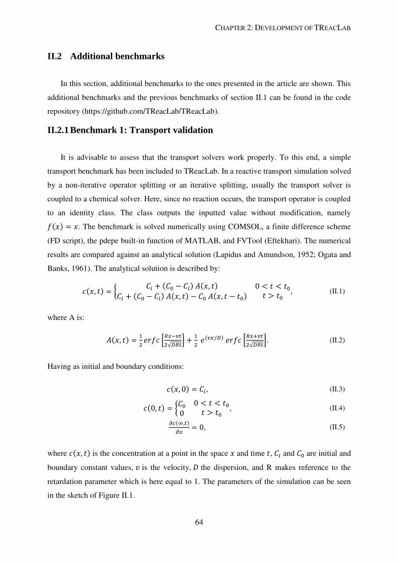
CHAPTER 2: DEVELOPMENT OF TREACLAB
64
II.2 Additional benchmarks
In this section, additional benchmarks to the ones presented in the article are shown. This
additional benchmarks and the previous benchmarks of section II.1 can be found in the code
repository (https://github.com/TReacLab/TReacLab).
II.2.1 Benchmark 1: Transport validation
It is advisable to assess that the transport solvers work properly. To this end, a simple
transport benchmark has been included to TReacLab. In a reactive transport simulation solved
by a non-iterative operator splitting or an iterative splitting, usually the transport solver is
coupled to a chemical solver. Here, since no reaction occurs, the transport operator is coupled
to an identity class. The class outputs the inputted value without modification, namely . The benchmark is solved numerically using COMSOL, a finite difference scheme
(FD script), the pdepe built-in function of MATLAB, and FVTool (Eftekhari). The numerical
results are compared against an analytical solution (Lapidus and Amundson, 1952; Ogata and
Banks, 1961). The analytical solution is described by:
, (II.1)
where A is:
. (II.2)
Having as initial and boundary conditions:
, (II.3)
, (II.4)
, (II.5)
where is the concentration at a point in the space and time , and are initial and
boundary constant values, is the velocity, the dispersion, and R makes reference to the
retardation parameter which is here equal to 1. The parameters of the simulation can be seen
in the sketch of Figure II.1.
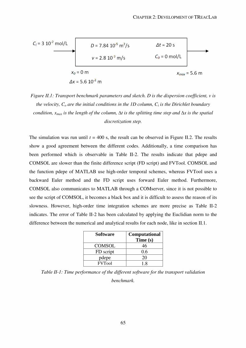
CHAPTER 2: DEVELOPMENT OF TREACLAB
65
Figure II.1: Transport benchmark parameters and sketch. D is the dispersion coefficient, v is
the velocity, Co are the initial conditions in the 1D column, Ci is the Dirichlet boundary
condition, xmax is the length of the column, ∆t is the splitting time step and ∆x is the spatial
discretization step.
The simulation was run until t = 400 s, the result can be observed in Figure II.2. The results
show a good agreement between the different codes. Additionally, a time comparison has
been performed which is observable in Table II-2. The results indicate that pdepe and
COMSOL are slower than the finite difference script (FD script) and FVTool. COMSOL and
the function pdepe of MATLAB use high-order temporal schemes, whereas FVTool uses a
backward Euler method and the FD script uses forward Euler method. Furthermore,
COMSOL also communicates to MATLAB through a COMserver, since it is not possible to
see the script of COMSOL, it becomes a black box and it is difficult to assess the reason of its
slowness. However, high-order time integration schemes are more precise as Table II-2
indicates. The error of Table II-2 has been calculated by applying the Euclidian norm to the
difference between the numerical and analytical results for each node, like in section II.1.
Software Computational
Time (s)
COMSOL 46
FD script 0.6
pdepe 20 FVTool 1.8
Table II-1: Time performance of the different software for the transport validation
benchmark.

CHAPTER 2: DEVELOPMENT OF TREACLAB
66
0,0 0,1 0,2 0,3 0,4 0,50,0
0,5
1,0
1,5
2,0
2,5
3,0
c (m
ol/
L)
x (m)
Analytical
pdepe
COMSOL
FD script
FVTool
x 10-2
Figure II.2: Concentration vs. distance at t = 400 of the different software and analytical
solution for the transport validation benchmark.
Software error
COMSOL 4.76 10-4
FD script 3 10-3
pdepe 8.24 10-4
FVTool 1.5 10-3
Table II-2: Error comparison between software and analytical solution for the transport
validation benchmark.
II.2.2 Benchmark 2: Cation exchange
This example presented first by Parkhurst and Appelo (1999b) has also been used by
other researches as a validation benchmark and analysis of numerical methods and approaches
(Amir and Kern, 2010; de Dieuleveult et al., 2009). The problem has been solved numerically
using the software coupling between FVTool and iPhreeqc, and also by PHREEQC alone in
order to have reference results.
The exercise simulates a 1D column containing initially a sodium-potassium-nitrate solution
in equilibrium with a cation exchanger. The column is flushed with a calcium-chloride
solution, leading to a series of speciation reaction and exchange reactions. The mass balance
of this exchange reactions is:
Log(K) = 0.8 (II.6)
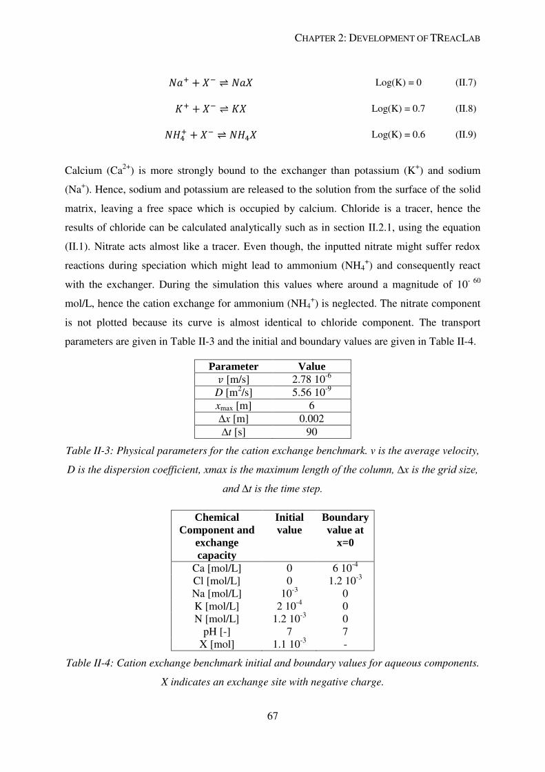
CHAPTER 2: DEVELOPMENT OF TREACLAB
67
Log(K) = 0 (II.7)
Log(K) = 0.7 (II.8)
Log(K) = 0.6 (II.9)
Calcium (Ca2+
) is more strongly bound to the exchanger than potassium (K+) and sodium
(Na+). Hence, sodium and potassium are released to the solution from the surface of the solid
matrix, leaving a free space which is occupied by calcium. Chloride is a tracer, hence the
results of chloride can be calculated analytically such as in section II.2.1, using the equation
(II.1). Nitrate acts almost like a tracer. Even though, the inputted nitrate might suffer redox
reactions during speciation which might lead to ammonium (NH4+) and consequently react
with the exchanger. During the simulation this values where around a magnitude of 10- 60
mol/L, hence the cation exchange for ammonium (NH4+) is neglected. The nitrate component
is not plotted because its curve is almost identical to chloride component. The transport
parameters are given in Table II-3 and the initial and boundary values are given in Table II-4.
Parameter Value [m/s] 2.78 10-6
D [m2/s] 5.56 10
-9
xmax [m] 6
∆x [m] 0.002
∆t [s] 90
Table II-3: Physical parameters for the cation exchange benchmark. v is the average velocity,
D is the dispersion coefficient, xmax is the maximum length of the column, ∆x is the grid size,
and ∆t is the time step.
Chemical
Component and
exchange
capacity
Initial
value
Boundary
value at
x=0
Ca [mol/L] 0 6 10-4
Cl [mol/L] 0 1.2 10-3
Na [mol/L] 10-3
0
K [mol/L] 2 10-4
0
N [mol/L] 1.2 10-3
0
pH [-] 7 7
X [mol] 1.1 10-3
-
Table II-4: Cation exchange benchmark initial and boundary values for aqueous components.
X indicates an exchange site with negative charge.

CHAPTER 2: DEVELOPMENT OF TREACLAB
68
In Figure II.3a, we compare the result of PHREEQC, given by a solid line, against the results
of FVTool-iPhreeqc coupling with a sequential splitting method, given by empty triangles. In
general a good agreement exists between results, but a slight shift between both results is
observable. This shift is attributable to the transport solver, since it also occurs in the tracer.
Other methods (additive, alternating, Strang, SWS) have also been performed, their results
match PHREEQC values as well. A similar comparison as in section II.1 for the "Ca"
component taking as reference the Strang method with the smallest splitting time step was
performed (Table II-5). The table shows independently of the method that smaller splitting
time steps lead to results in better accordance with the reference results, therefore we
conclude that the methods are consistent.
Figure II.3b shows the concentration of the components at the outflow. After one pore volume
(8 h), the concentration of the tracer ("Cl") reaches the outflow of the column. The release of
all the "K" component is delayed in comparison to "Na" , since "K" bounds stronger (because
of larger log K in the exchange reaction). Once there is no more "Na" in the exchanger the
amount of "Ca" that reaches the outflow starts to increase. Finally, once all the exchange sites
have been occupied by "Ca", namely when "K" is out of the 1D column, "Ca" reaches its
steady-state concentration equal as in the input side of the column.
0,02 0,04 0,06 0,080
0,4
0,8
1,2
0
C (
mol/
L)
x (m)
Ca
Cl
Na
K
x 10-3
a)
0 5 10 15 20
0,4
0,8
1,2
0
b) x 10-3
C (
mol/
L)
Time (h)
Figure II.3: a) Component concentration vs length at time t = 3.6 h, b) concentration at the
end of the column vs time. The results of PHREEQC are represented by a solid line, while the
results of the coupling between FVTool and iPhreeqc are given by empty triangles.
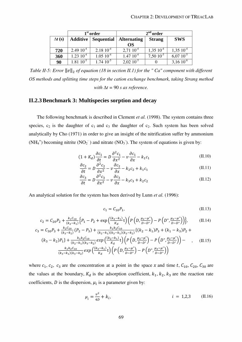
CHAPTER 2: DEVELOPMENT OF TREACLAB
69
1st
order 2nd
order
∆t (s) Additive Sequential Alternating
OS
Strang SWS
720 2.49 10-4
2.18 10-4
2,71 10-4
1,35 10-4
1,35 10-4
360 1.23 10-4
1.05 10-4
1.47 10-4
7,50 10-5
6,07 10-5
90 1.81 10-5
1.74 10-5
2,02 10-5
0 3,16 10-6
Table II-5: Error of equation (18 in section II.1) for the " Ca" component with different
OS methods and splitting time steps for the cation exchange benchmark, taking Strang method
with ∆t = 90 s as reference.
II.2.3 Benchmark 3: Multispecies sorption and decay
The following benchmark is described in Clement et al. (1998). The system contains three
species, c2 is the daughter of c1 and c3 the daughter of c2. Such system has been solved
analytically by Cho (1971) in order to give an insight of the nitrification suffer by ammonium
(NH4+) becoming nitrite (NO2
- ) and nitrate (NO3
-). The system of equations is given by:
(II.10)
(II.11)
(II.12)
An analytical solution for the system has been derived by Lunn et al. (1996):
, (II.13)
, (II.14)
, (II.15)
where , , are the concentration at a point in the space and time , , , are
the values at the boundary, is the adsorption coefficient, , , are the reaction rate
coefficients, is the dispersion, is a parameter given by:
, (II.16)

CHAPTER 2: DEVELOPMENT OF TREACLAB
70
being the velocity, the symbol * in and indicates that these parameters are divided by
1/(1+ ), and is a function such as:
, (II.17)
where and for are and respectively and for , and are and
respectively. The parameters for the simulation are given in Table II-6. The boundary
conditions of the 1D column are:
for x = 0 (II.18)
for xmax (II.19)
Parameter Value [cm/h] 0.1
D [cm2/h] 0.018
xmax [cm] 40 1 [h-1
] 0.05 [h-1
] 0.03 [h-1
] 0.02
∆x [cm] 0.5
∆t [h] 0.5
Table II-6: Physical and chemical parameters for the multispecies sorption and decay
benchmark. is the average velocity, D is the dispersion coefficient, xmax is the maximum
length of the column, ∆x is the grid size, ∆t is the time step, Kd is the adsorption coefficient,
and ki with i = 1,2, 3 are the reaction rates.
Figure II.4 shows the analytical solution and numerical solution at t = 100 h with an additive
splitting and t = 200 h with a symmetrically weighted splitting. The numerical solution is
obtained with the software coupling between a finite difference script for the transport
operator and ode45 built-in function of MATLAB for the reaction operator. Other numerical
splitting scheme (sequential, alternating, Strang) show similar trends. In Figure II.4a, it is
observable that the numerical profiles of and are slightly advanced in comparison to the
analytical profiles. After 100 h (Figure II.4b), the match between the numerical and analytical
profiles is more accurate.

CHAPTER 2: DEVELOPMENT OF TREACLAB
71
0 10 200,0
0,2
0,4
0,6
0,8
1,0
C (
mo
l/L
)
x (m)
c1 R
c1 OS
c2 R
c2 OS
c3 R
c3 OS
T = 100 h (Additive splitting)a)
0 10 20 300,0
0,2
0,4
0,6
0,8
1,0b)
C (
mo
l/L
)
x (m)
c1 R
c1 OS
c2 R
c2 OS
c3 R
c3 OS)
T = 200 h (SWS)
Figure II.4: Concentration vs length plots at a) t = 100 h and b) t = 200 h. The analytical
solution is depicted by a solid line, in the legend it is accompanied by a R. The numerical
solution is depicted by an empty triangle, in the legend accompanied by 'OS' (operator
splitting). The numerical approach used is the additive splitting.
II.3 External transport and geochemical plugged codes
In order to do the simulations of this chapter of the thesis, several codes have been
employed. Therefore, a section is dedicated to give an insight into these codes.
II.3.1 Transport codes
Three external transport codes have been used as transport operators: COMSOL, the
pdepe built-in function of MATLAB and FVTool. Furthermore, a simple finite difference
script has been developed.
II.3.1.1 COMSOL
COMSOL Multiphysics (COMSOL, 2012) is a commercial finite element method
software used in various physics and engineering problems allowing several types of
analyses: stationary, time-dependent, eigenfrequency, eigenvalue and also wide variety of
customizable geometries. In COMSOL it is possible to introduce coupled systems of PDEs,
but several add-on modules exist. The modules are categorized according to the application
area. Every module incorporates the classical system of equations of their respective area.

CHAPTER 2: DEVELOPMENT OF TREACLAB
72
COMSOL uses an interactive environment for the modelization of the problem. Nevertheless,
it can be run by scripts programs written in MATLAB thanks to the Livelink for MATLAB
(COMSOL, 2010). It is a client-server mode where MATLAB is the client and COMSOL the
server which uses a TCP/ICP communication protocol.
There are three main ways to use COMSOL with MATLAB. The user can create the whole
model in COMSOL, namely physical parameters, mesh and other pre-processing features, and
then import the model into MATLAB for further use or just post-processing purposes. The
user can also call MATLAB functions from COMSOL. Finally, the user can create the whole
model from scratch in MATLAB by calling the suitable application interface program
functions. In our case, since we use a simple geometry (1D) and just one physical module of
COMSOL called solute transport, we have chosen to create the model from scratch, using
only MATLAB and calling the interface program functions of COMSOL. The reason for that
is that we want to keep a generic software which can handle different external software
couplings and is not embedded with specific software. The equation of the solute transport
physical module of COMSOL is:
, (II.20)
where is the porosity, is the bulk density, c the concentration, , , and are the rate
constant, the solid concentration, and the density of the solid concentration respectively,
related to one of the following sorption models: Langmuir, Freundlich or user-defined. is
the effective diffusion and the dispersion tensor, is the velocity, stands for kinetic
chemical reaction which might be added and for the sink/source terms.
The COMSOL model allows changes of porosity due to sorption, but in this work we do not
make use of this capability. Furthermore, no kinetic reaction module of COMSOL have been
added to the transport equation. The reason resides on the fact that we separate the chemical
operator from the transport operator, although the possibility might be considered in other
projects.
II.3.1.2 FVTool
FVTool is an open-source objected-oriented toolbox written in MATLAB which solves
mass conservative equations using finite volume methods. It was inspired by another
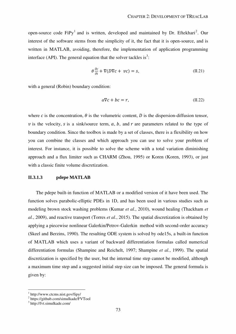
CHAPTER 2: DEVELOPMENT OF TREACLAB
73
open-source code FiPy1 and is written, developed and maintained by Dr. Eftekhari
2. Our
interest of the software stems from the simplicity of it, the fact that it is open-source, and is
written in MATLAB, avoiding, therefore, the implementation of application programming
interface (API). The general equation that the solver tackles is3:
, (II.21)
with a general (Robin) boundary condition:
, (II.22)
where is the concentration, is the volumetric content, is the dispersion-diffusion tensor, is the velocity, is a sink/source term, , , and are parameters related to the type of
boundary condition. Since the toolbox is made by a set of classes, there is a flexibility on how
you can combine the classes and which approach you can use to solve your problem of
interest. For instance, it is possible to solve the scheme with a total variation diminishing
approach and a flux limiter such as CHARM (Zhou, 1995) or Koren (Koren, 1993), or just
with a classic finite volume discretization.
II.3.1.3 pdepe MATLAB
The pdepe built-in function of MATLAB or a modified version of it have been used. The
function solves parabolic-elliptic PDEs in 1D, and has been used in various studies such as
modeling brown stock washing problems (Kumar et al., 2010), wound healing (Thackham et
al., 2009), and reactive transport (Torres et al., 2015). The spatial discretization is obtained by
applying a piecewise nonlinear Galerkin/Petrov-Galerkin method with second-order accuracy
(Skeel and Berzins, 1990). The resulting ODE system is solved by ode15s, a built-in function
of MATLAB which uses a variant of backward differentiation formulas called numerical
differentiation formulas (Shampine and Reichelt, 1997; Shampine et al., 1999). The spatial
discretization is specified by the user, but the internal time step cannot be modified, although
a maximum time step and a suggested initial step size can be imposed. The general formula is
given by:
1 http://www.ctcms.nist.gov/fipy/
2 https://github.com/simulkade/FVTool
3 http://fvt.simulkade.com/

CHAPTER 2: DEVELOPMENT OF TREACLAB
74
, (II.23)
where and are the spatial and time variables respectively, and is the dependent variable,
which in our case is either the species or the component concentrations. The parameter can
vary from 0 to 2 in order to represent the symmetry of the problem (slab , cylindrical , or spherical symmetry ) in our case it has kept to 0. To use the pdepe
solver, 3 functions have to be defined: a) one giving the values of ,
and , b) another giving the initial conditions , and finally c) one giving the
boundary conditions by stating the values of and at the beginning and end of
the 1D system. Table II-7 illustrates values of and according to the type of boundary
conditions.
a)
,
(II.24) , .
b) (II.25)
c) (II.26)
Type Formula
Dirichlet
Neumann
Cauchy or Robin
Table II-7: Implementation of boundary conditions in the pdepe built-in function of MATLAB
(Shafei, 2012).
In section II.2.1, we have employed the default time integration of the pdepe function, but in
all the other benchmarks (section II.1) we have withdrawn the spatial discretization given by
the MATLAB solver and applied a forward Euler scheme (first-order time explicit scheme).
Consequently, it is usually less accurate than the default scheme which is a numerical
differentiation formula scheme. Although, the application of forward Euler scheme results in
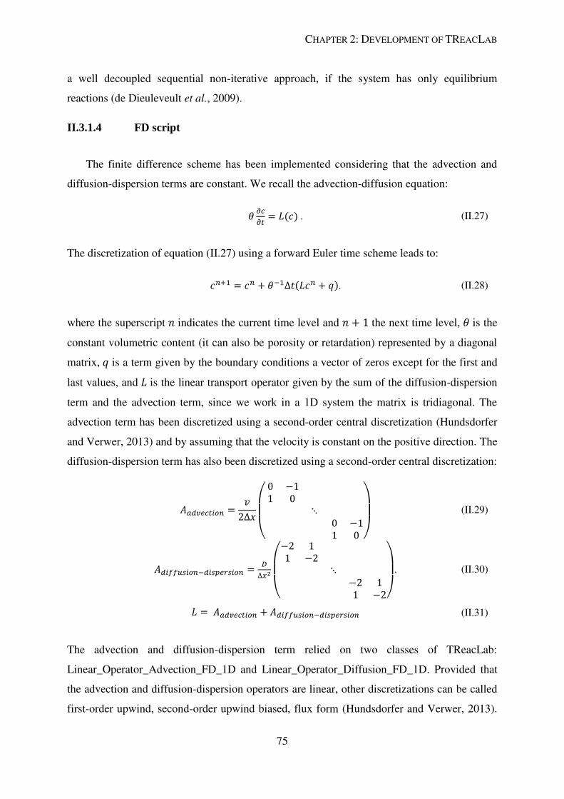
CHAPTER 2: DEVELOPMENT OF TREACLAB
75
a well decoupled sequential non-iterative approach, if the system has only equilibrium
reactions (de Dieuleveult et al., 2009).
II.3.1.4 FD script
The finite difference scheme has been implemented considering that the advection and
diffusion-dispersion terms are constant. We recall the advection-diffusion equation:
. (II.27)
The discretization of equation (II.27) using a forward Euler time scheme leads to:
. (II.28)
where the superscript indicates the current time level and the next time level, is the
constant volumetric content (it can also be porosity or retardation) represented by a diagonal
matrix, is a term given by the boundary conditions a vector of zeros except for the first and
last values, and is the linear transport operator given by the sum of the diffusion-dispersion
term and the advection term, since we work in a 1D system the matrix is tridiagonal. The
advection term has been discretized using a second-order central discretization (Hundsdorfer
and Verwer, 2013) and by assuming that the velocity is constant on the positive direction. The
diffusion-dispersion term has also been discretized using a second-order central discretization:
(II.29)
. (II.30)
(II.31)
The advection and diffusion-dispersion term relied on two classes of TReacLab:
Linear_Operator_Advection_FD_1D and Linear_Operator_Diffusion_FD_1D. Provided that
the advection and diffusion-dispersion operators are linear, other discretizations can be called
first-order upwind, second-order upwind biased, flux form (Hundsdorfer and Verwer, 2013).
CHAPTER 2: DEVELOPMENT OF TREACLAB
76
Unfortunately, we have not applied any of these other discretizations in the presented
benchmarks.
Since coupling methods can sometimes force the use of certain types of numerical schemes
such as an implicit or explicit approach. When we applied the SIA CC scheme, we descritize
the advection-diffusion equation with a backward Euler time discretization and add a source
parameter :
, (II.32)
where is here a difference given by the fix components at initial and final state of each
splitting time step, .
II.3.2 Geochemical codes
Most of the geochemical system presented on the tests have been solved by applying
codes based on PHREEQC: iPhreeqc and PhreeqcRM. Although, simple chemistry such as in
section II.2.3 have been solved by analytical solutions, explicit or implicit first-order Euler
scheme, or the ode45 function of MATLAB. In the following, we only described the
PHREEQC's set solvers.
II.3.2.1 PHREEQC, iPhreeqc, and PhreeqcRM
PHREEQC (pH-REdox-EQuilibrium in C programming language) is a free, open-source
state-of-art geochemical package of the USGS (Parkhurst and Appelo, 1999b). PHREEQC
has several databases and allows to use user-defined database or modified previously existing
databases. It can work with different aqueous models: Lawrence Livermore National
Laboratory model, WATEQ4F model, Pitzer specific-ion-interaction aqueous model, and the
specific ion interaction theory aqueous models. The software accounts for a series of
geochemical equilibrium equations such aqueous solution interacting with minerals, gases,
solid solutions, exchangers, and sorption surfaces. PHREEQC also includes kinetic reactions
and 1D reactive transport.
PHREEQC formulation for every chemical equilibrium problem derives from a set of
equations (Parkhurst and Appelo, 1999a):
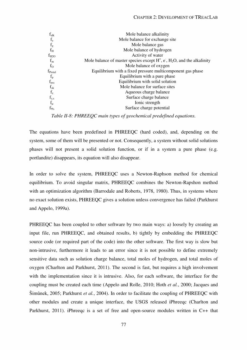
CHAPTER 2: DEVELOPMENT OF TREACLAB
77
falk Mole balance alkalinity
fe Mole balance for exchange site
fg Mole balance gas
fH Mole balance of hydrogen
fH2O Activity of water
fm Mole balance of master species except H+, e
-, H2O, and the alkalinity
fO Mole balance of oxygen
fPtotal Equilibrium with a fixed pressure multicomponent gas phase
fp Equilibrium with a pure phase
fpss Equilibrium with solid solution
fsk Mole balance for surface sites
fz Aqueous charge balance
fz,s Surface charge balance
fµ Ionic strength
fΨs Surface charge potential
Table II-8: PHREEQC main types of geochemical predefined equations.
The equations have been predefined in PHREEQC (hard coded), and, depending on the
system, some of them will be presented or not. Consequently, a system without solid solutions
phases will not present a solid solution function, or if in a system a pure phase (e.g.
portlandite) disappears, its equation will also disappear.
In order to solve the system, PHREEQC uses a Newton-Raphson method for chemical
equilibrium. To avoid singular matrix, PHREEQC combines the Newton-Rapshon method
with an optimization algorithm (Barrodale and Roberts, 1978, 1980). Thus, in systems where
no exact solution exists, PHREEQC gives a solution unless convergence has failed (Parkhurst
and Appelo, 1999a).
PHREEQC has been coupled to other software by two main ways: a) loosely by creating an
input file, run PHREEQC, and obtained results, b) tightly by embedding the PHREEQC
source code (or required part of the code) into the other software. The first way is slow but
non-intrusive, furthermore it leads to an error since it is not possible to define extremely
sensitive data such as solution charge balance, total moles of hydrogen, and total moles of
oxygen (Charlton and Parkhurst, 2011). The second is fast, but requires a high involvement
with the implementation since it is intrusive. Also, for each software, the interface for the
coupling must be created each time (Appelo and Rolle, 2010; Hoth et al., 2000; Jacques and
Šimůnek, 2005; Parkhurst et al., 2004). In order to facilitate the coupling of PHREEQC with
other modules and create a unique interface, the USGS released iPhreeqc (Charlton and
Parkhurst, 2011). iPhreeqc is a set of free and open-source modules written in C++ that
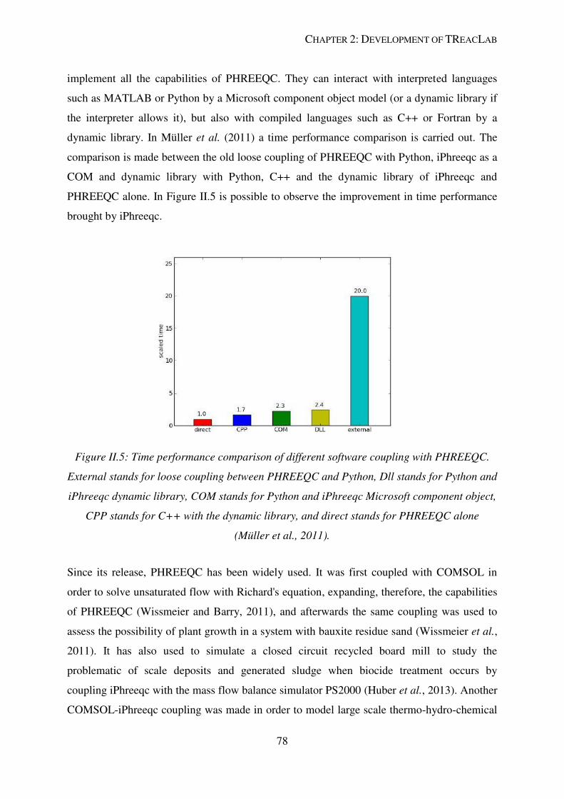
CHAPTER 2: DEVELOPMENT OF TREACLAB
78
implement all the capabilities of PHREEQC. They can interact with interpreted languages
such as MATLAB or Python by a Microsoft component object model (or a dynamic library if
the interpreter allows it), but also with compiled languages such as C++ or Fortran by a
dynamic library. In Müller et al. (2011) a time performance comparison is carried out. The
comparison is made between the old loose coupling of PHREEQC with Python, iPhreeqc as a
COM and dynamic library with Python, C++ and the dynamic library of iPhreeqc and
PHREEQC alone. In Figure II.5 is possible to observe the improvement in time performance
brought by iPhreeqc.
Figure II.5: Time performance comparison of different software coupling with PHREEQC.
External stands for loose coupling between PHREEQC and Python, Dll stands for Python and
iPhreeqc dynamic library, COM stands for Python and iPhreeqc Microsoft component object,
CPP stands for C++ with the dynamic library, and direct stands for PHREEQC alone
(Müller et al., 2011).
Since its release, PHREEQC has been widely used. It was first coupled with COMSOL in
order to solve unsaturated flow with Richard's equation, expanding, therefore, the capabilities
of PHREEQC (Wissmeier and Barry, 2011), and afterwards the same coupling was used to
assess the possibility of plant growth in a system with bauxite residue sand (Wissmeier et al.,
2011). It has also used to simulate a closed circuit recycled board mill to study the
problematic of scale deposits and generated sludge when biocide treatment occurs by
coupling iPhreeqc with the mass flow balance simulator PS2000 (Huber et al., 2013). Another
COMSOL-iPhreeqc coupling was made in order to model large scale thermo-hydro-chemical
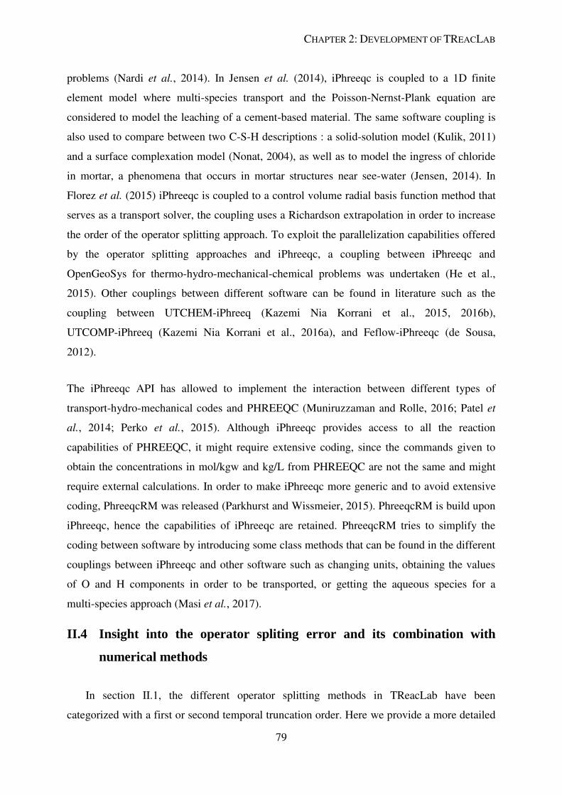
CHAPTER 2: DEVELOPMENT OF TREACLAB
79
problems (Nardi et al., 2014). In Jensen et al. (2014), iPhreeqc is coupled to a 1D finite
element model where multi-species transport and the Poisson-Nernst-Plank equation are
considered to model the leaching of a cement-based material. The same software coupling is
also used to compare between two C-S-H descriptions : a solid-solution model (Kulik, 2011)
and a surface complexation model (Nonat, 2004), as well as to model the ingress of chloride
in mortar, a phenomena that occurs in mortar structures near see-water (Jensen, 2014). In
Florez et al. (2015) iPhreeqc is coupled to a control volume radial basis function method that
serves as a transport solver, the coupling uses a Richardson extrapolation in order to increase
the order of the operator splitting approach. To exploit the parallelization capabilities offered
by the operator splitting approaches and iPhreeqc, a coupling between iPhreeqc and
OpenGeoSys for thermo-hydro-mechanical-chemical problems was undertaken (He et al.,
2015). Other couplings between different software can be found in literature such as the
coupling between UTCHEM-iPhreeq (Kazemi Nia Korrani et al., 2015, 2016b),
UTCOMP-iPhreeq (Kazemi Nia Korrani et al., 2016a), and Feflow-iPhreeqc (de Sousa,
2012).
The iPhreeqc API has allowed to implement the interaction between different types of
transport-hydro-mechanical codes and PHREEQC (Muniruzzaman and Rolle, 2016; Patel et
al., 2014; Perko et al., 2015). Although iPhreeqc provides access to all the reaction
capabilities of PHREEQC, it might require extensive coding, since the commands given to
obtain the concentrations in mol/kgw and kg/L from PHREEQC are not the same and might
require external calculations. In order to make iPhreeqc more generic and to avoid extensive
coding, PhreeqcRM was released (Parkhurst and Wissmeier, 2015). PhreeqcRM is build upon
iPhreeqc, hence the capabilities of iPhreeqc are retained. PhreeqcRM tries to simplify the
coding between software by introducing some class methods that can be found in the different
couplings between iPhreeqc and other software such as changing units, obtaining the values
of O and H components in order to be transported, or getting the aqueous species for a
multi-species approach (Masi et al., 2017).
II.4 Insight into the operator spliting error and its combination with
numerical methods
In section II.1, the different operator splitting methods in TReacLab have been
categorized with a first or second temporal truncation order. Here we provide a more detailed

CHAPTER 2: DEVELOPMENT OF TREACLAB
80
analysis in order to answer how the operator splitting error is obtained. To that purpose, we
assume that all the reactions are differentiable kinetic functions. The first section addresses
the error introduced by the sequential splitting using Taylor series, the same approach might
be applied to other operator splitting methods. The second section builds upon the concepts
developed in the first part to show a more practical use.
II.4.1 Error of the operator splitting methods
We consider an abstract initial value problem:
, , , (II.33)
In order to apply an operator scheme, the linear or non-linear function is
decomposed into the sum of two simpler operators: which are assumed to be solved exactly. Usually, in reactive transport, the operators are
transport (e.g. ) and chemistry (e.g. ), but different decompositions are possible (Clement
et al., 1998). We analyze the local error of the sequential splitting for its first iteration, being
the splitting time step (Geiser, 2009):
, , , (II.34)
, , (II.35)
. (II.36)
The local truncation error is defined by the difference between the exact solution and the split
solution:
, (II.37)
where is the local truncation error, is the exact solution after one splitting time step and is the splitting solution after one splitting time step. The same convention as Csomós et al.
(2005) is followed, namely:
, (II.38)

CHAPTER 2: DEVELOPMENT OF TREACLAB
81
with some . Then, it is said that the splitting scheme is pth-order scheme. In order to prove that
the sequential splitting has a first-order local error, we expand the exact solution around t = 0 using
Taylor series:
, (II.39)
combining equation (II.33), equation (II.39) and knowing that , leads to:
(II.40)
The functions , and theirs derivatives are evaluated at (0, ). We now apply Taylor
series at t = 0 to the sequential splitting method (equation (II.34)-(II.36)). Such that:
. (II.41)
Notice that in equation (II.41) in comparison to equation (II.40), and its derivatives are
evaluated at (0, ). Before calculating the error (equation (II.37)), since as
stated in equation (II.35), the terms , , and
must be expanded and substituted in equation (II.41). Now, we expand :
. (II.42)
Here, and its derivatives are evaluated at (0, ). Now, we should expand , and . Since:
, (II.43)
and with , we can extend , and :
. (II.44)
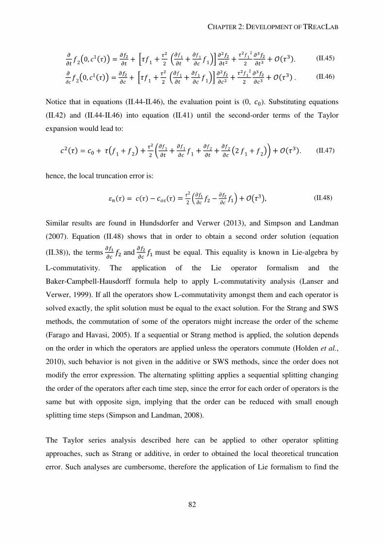
CHAPTER 2: DEVELOPMENT OF TREACLAB
82
. (II.45)
. (II.46)
Notice that in equations (II.44-II.46), the evaluation point is (0, ). Substituting equations
(II.42) and (II.44-II.46) into equation (II.41) until the second-order terms of the Taylor
expansion would lead to:
. (II.47)
hence, the local truncation error is:
, (II.48)
Similar results are found in Hundsdorfer and Verwer (2013), and Simpson and Landman
(2007). Equation (II.48) shows that in order to obtain a second order solution (equation
(II.38)), the terms and
must be equal. This equality is known in Lie-algebra by
L-commutativity. The application of the Lie operator formalism and the
Baker-Campbell-Hausdorff formula help to apply L-commutativity analysis (Lanser and
Verwer, 1999). If all the operators show L-commutativity amongst them and each operator is
solved exactly, the split solution must be equal to the exact solution. For the Strang and SWS
methods, the commutation of some of the operators might increase the order of the scheme
(Farago and Havasi, 2005). If a sequential or Strang method is applied, the solution depends
on the order in which the operators are applied unless the operators commute (Holden et al.,
2010), such behavior is not given in the additive or SWS methods, since the order does not
modify the error expression. The alternating splitting applies a sequential splitting changing
the order of the operators after each time step, since the error for each order of operators is the
same but with opposite sign, implying that the order can be reduced with small enough
splitting time steps (Simpson and Landman, 2008).
The Taylor series analysis described here can be applied to other operator splitting
approaches, such as Strang or additive, in order to obtained the local theoretical truncation
error. Such analyses are cumbersome, therefore the application of Lie formalism to find the
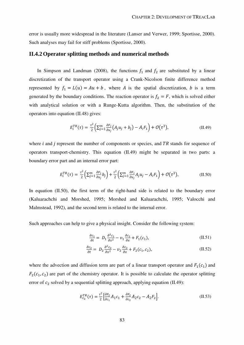
CHAPTER 2: DEVELOPMENT OF TREACLAB
83
error is usually more widespread in the literature (Lanser and Verwer, 1999; Sportisse, 2000).
Such analyses may fail for stiff problems (Sportisse, 2000).
II.4.2 Operator splitting methods and numerical methods
In Simpson and Landman (2008), the functions and are substituted by a linear
discretization of the transport operator using a Crank-Nicolson finite difference method
represented by , where is the spatial discretization, is a term
generated by the boundary conditions. The reaction operator is , which is solved either
with analytical solution or with a Runge-Kutta algorithm. Then, the substitution of the
operators into equation (II.48) gives:
, (II.49)
where and represent the number of components or species, and stands for sequence of
operators transport-chemistry. This equation (II.49) might be separated in two parts: a
boundary error part and an internal error part:
, (II.50)
In equation (II.50), the first term of the right-hand side is related to the boundary error
(Kaluarachchi and Morshed, 1995; Morshed and Kaluarachchi, 1995; Valocchi and
Malmstead, 1992), and the second term is related to the internal error.
Such approaches can help to give a physical insight. Consider the following system:
, (II.51)
, (II.52)
where the advection and diffusion term are part of a linear transport operator and and are part of the chemistry operator. It is possible to calculate the operator splitting
error of solved by a sequential splitting approach, applying equation (II.49):
. (II.53)
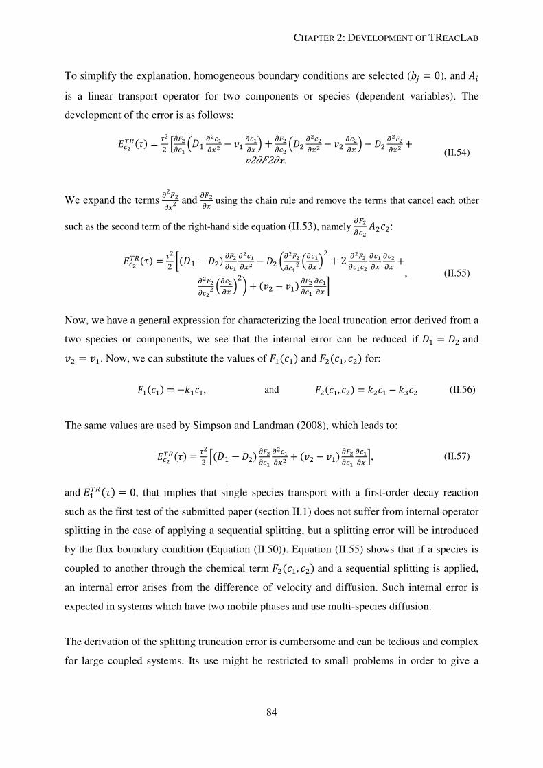
CHAPTER 2: DEVELOPMENT OF TREACLAB
84
To simplify the explanation, homogeneous boundary conditions are selected ( ), and is a linear transport operator for two components or species (dependent variables). The
development of the error is as follows:
2 2 .
(II.54)
We expand the terms and
using the chain rule and remove the terms that cancel each other
such as the second term of the right-hand side equation (II.53), namely :
, (II.55)
Now, we have a general expression for characterizing the local truncation error derived from a
two species or components, we see that the internal error can be reduced if and . Now, we can substitute the values of and for:
, and (II.56)
The same values are used by Simpson and Landman (2008), which leads to:
, (II.57)
and , that implies that single species transport with a first-order decay reaction
such as the first test of the submitted paper (section II.1) does not suffer from internal operator
splitting in the case of applying a sequential splitting, but a splitting error will be introduced
by the flux boundary condition (Equation (II.50)). Equation (II.55) shows that if a species is
coupled to another through the chemical term and a sequential splitting is applied,
an internal error arises from the difference of velocity and diffusion. Such internal error is
expected in systems which have two mobile phases and use multi-species diffusion.
The derivation of the splitting truncation error is cumbersome and can be tedious and complex
for large coupled systems. Its use might be restricted to small problems in order to give a
CHAPTER 2: DEVELOPMENT OF TREACLAB
85
mathematical insight into the factors that can produce errors. For larger systems, symbolic
computation might be a solution.
86
CHAPTER 3: ATMOSPHERIC CARBONATION
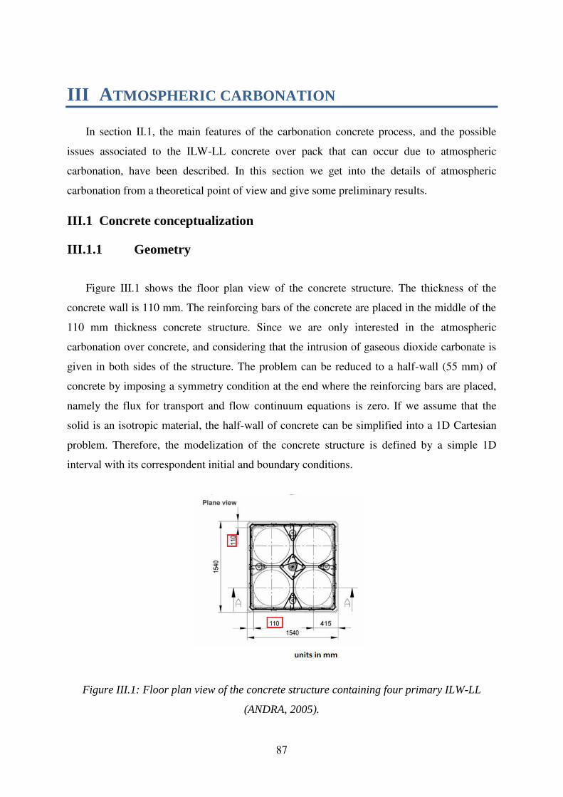
87
III ATMOSPHERIC CARBONATION
In section II.1, the main features of the carbonation concrete process, and the possible
issues associated to the ILW-LL concrete over pack that can occur due to atmospheric
carbonation, have been described. In this section we get into the details of atmospheric
carbonation from a theoretical point of view and give some preliminary results.
III.1 Concrete conceptualization
III.1.1 Geometry
Figure III.1 shows the floor plan view of the concrete structure. The thickness of the
concrete wall is 110 mm. The reinforcing bars of the concrete are placed in the middle of the
110 mm thickness concrete structure. Since we are only interested in the atmospheric
carbonation over concrete, and considering that the intrusion of gaseous dioxide carbonate is
given in both sides of the structure. The problem can be reduced to a half-wall (55 mm) of
concrete by imposing a symmetry condition at the end where the reinforcing bars are placed,
namely the flux for transport and flow continuum equations is zero. If we assume that the
solid is an isotropic material, the half-wall of concrete can be simplified into a 1D Cartesian
problem. Therefore, the modelization of the concrete structure is defined by a simple 1D
interval with its correspondent initial and boundary conditions.
Figure III.1: Floor plan view of the concrete structure containing four primary ILW-LL
(ANDRA, 2005).
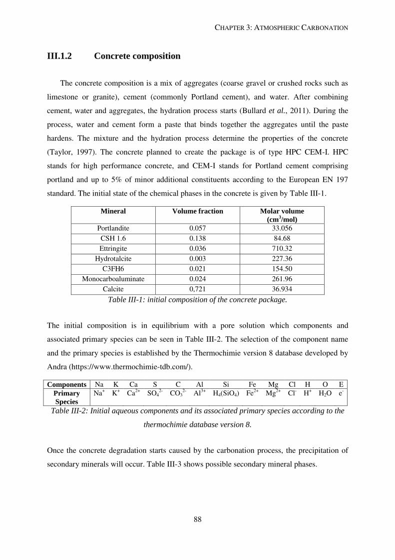
CHAPTER 3: ATMOSPHERIC CARBONATION
88
III.1.2 Concrete composition
The concrete composition is a mix of aggregates (coarse gravel or crushed rocks such as
limestone or granite), cement (commonly Portland cement), and water. After combining
cement, water and aggregates, the hydration process starts (Bullard et al., 2011). During the
process, water and cement form a paste that binds together the aggregates until the paste
hardens. The mixture and the hydration process determine the properties of the concrete
(Taylor, 1997). The concrete planned to create the package is of type HPC CEM-I. HPC
stands for high performance concrete, and CEM-I stands for Portland cement comprising
portland and up to 5% of minor additional constituents according to the European EN 197
standard. The initial state of the chemical phases in the concrete is given by Table III-1.
Mineral Volume fraction Molar volume
(cm3/mol)
Portlandite 0.057 33.056
CSH 1.6 0.138 84.68
Ettringite 0.036 710.32
Hydrotalcite 0.003 227.36
C3FH6 0.021 154.50
Monocarboaluminate 0.024 261.96
Calcite 0,721 36.934
Table III-1: initial composition of the concrete package.
The initial composition is in equilibrium with a pore solution which components and
associated primary species can be seen in Table III-2. The selection of the component name
and the primary species is established by the Thermochimie version 8 database developed by
Andra (https://www.thermochimie-tdb.com/).
Components Na K Ca S C Al Si Fe Mg Cl H O E
Primary
Species
Na+
K+
Ca2+
SO42-
CO32-
Al3+
H4(SiO4) Fe2+
Mg2+
Cl- H
+ H2O e
-
Table III-2: Initial aqueous components and its associated primary species according to the
thermochimie database version 8.
Once the concrete degradation starts caused by the carbonation process, the precipitation of
secondary minerals will occur. Table III-3 shows possible secondary mineral phases.
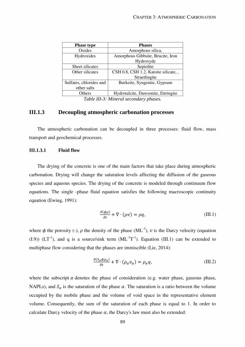
CHAPTER 3: ATMOSPHERIC CARBONATION
89
Phase type Phases
Oxides Amorphous silica,
Hydroxides Amorphous Gibbsite, Brucite, Iron
Hydroxyde
Sheet silicates Sepiolite
Other silicates CSH 0.8, CSH 1.2, Katoite silicate, ,
Straetlingite
Sulfates, chlorides and
other salts
Burkeite, Syngenite, Gypsum
Others Hydrotalcite, Dawsonite, Ettringite
Table III-3: Mineral secondary phases.
III.1.3 Decoupling atmospheric carbonation processes
The atmospheric carbonation can be decoupled in three processes: fluid flow, mass
transport and geochemical processes.
III.1.3.1 Fluid flow
The drying of the concrete is one of the main factors that take place during atmospheric
carbonation. Drying will change the saturation levels affecting the diffusion of the gaseous
species and aqueous species. The drying of the concrete is modeled through continuum flow
equations. The single -phase fluid equation satisfies the following macroscopic continuity
equation (Ewing, 1991):
, (III.1)
where the porosity (-), the density of the phase (ML-3
), is the Darcy velocity (equation
(I.9)) (LT-1
), and q is a source/sink term (ML-3
T-1
). Equation (III.1) can be extended to
multiphase flow considering that the phases are immiscible (Lie, 2014):
, (III.2)
where the subscript denotes the phase of consideration (e.g. water phase, gaseous phase,
NAPLs), and is the saturation of the phase . The saturation is a ratio between the volume
occupied by the mobile phase and the volume of void space in the representative element
volume. Consequently, the sum of the saturation of each phase is equal to 1. In order to
calculate Darcy velocity of the phase , the Darcy's law must also be extended:
CHAPTER 3: ATMOSPHERIC CARBONATION
90
. (III.3)
The parameters are the same as that of equation (I.9) for the corresponding phase , except
for which is the phase permeability:
, (III.4)
where is the intrinsic permeability that is affected by changes in the solid matrix such as
dissolution and precipitation (Samson and Marchand, 2006), and is the relative
permeability which depends on the saturation of the phase. The relative permeability accounts
for the flow paths of the phase when other phases are presented, it ranges from 0 (no phase ) to 1 (fully saturation). The simplest permeability models is Corey (Corey, 1954):
, (III.5)
, (III.6)
where the terms , , , are fitting parameters and is the normalized (or effective)
water content:
. (III.7)
Other common models for the relative permeability are the Brooks-Corey functions (Brooks
and Corey, 1964):
, (III.8)
, (III.9)
and the van Genuchten-Mualem model (Van Genuchten, 1980):
, (III.10)
, (III.11)
where the parameters , , , , and depend on the soil properties.

CHAPTER 3: ATMOSPHERIC CARBONATION
91
In a carbonation problem, we face a system made up of two mobile phases: gaseous and liquid
(water). Then, If we coupled equation (III.2) and (III.3), the system is described by:
, (III.12)
. (III.13)
The subscript stands for liquid and the subscript for gas. The system counts with four
dependent variables , , , and . In order two work with just two variables, two
constitutive relationships are needed. The relationship between saturations have been already
commented:
. (III.14)
The other arises from the interface between the liquid and the gaseous phase, known as
capillary force (Miller et al., 1998). On a molecular level, when two fluids are present in a
pore space, the molecules of one fluid are attracted to the solid by adhesive forces, such fluid
is known as the wetting phase fluid. The molecules of the other fluid are attracted to the
wetting fluid by cohesive forces, such fluid is known as the non-wetting phase fluid. In a
hydrophilic porous media like concrete, water is the wetting phase (Szymkiewicz, 2012). The
difference of pressure at the fluid-fluid interface gives rise to the capillary pressure:
. (III.15)
The capillary pressure is assumed to be function of the liquid saturation, (Chen et al.,
1994). The relationship between the capillary pressure and the water saturation shows
hysteresis (Figure III.2), the hysteresis might be explained by the different value of the
wetting angle when the fluid advances or recedes, the pore-scale trapping of air and by the
ink-bottle effect (Pinder and Gray, 2008). An example of hysteresis models are the Parlange
(1976) model, the Likos and Lu (2004) model, or Zhou (2015). In this work we do not use
hysteric models and will work only with the capillary curve which are monotonic functions.
The most common curves are the Brooks and Corey (1964):
(III.16)
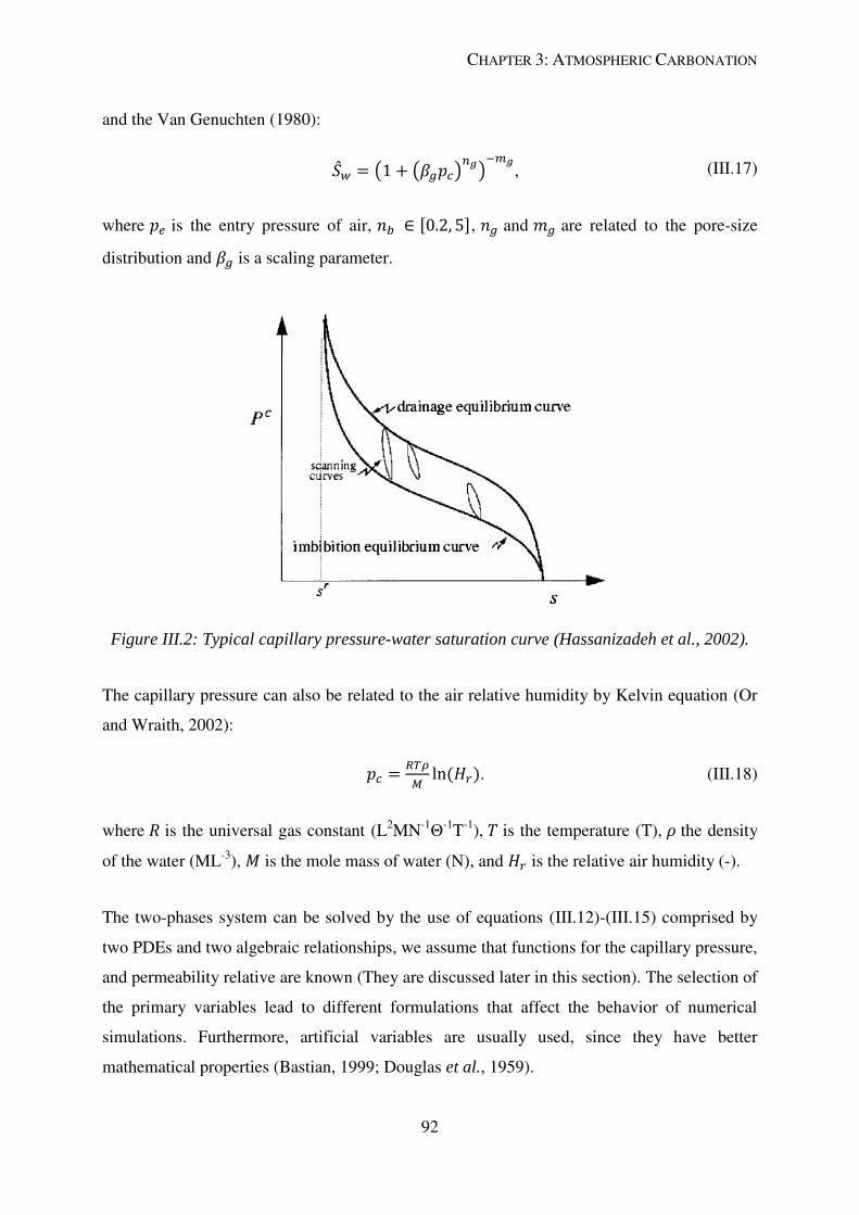
CHAPTER 3: ATMOSPHERIC CARBONATION
92
and the Van Genuchten (1980):
, (III.17)
where is the entry pressure of air, , and are related to the pore-size
distribution and is a scaling parameter.
Figure III.2: Typical capillary pressure-water saturation curve (Hassanizadeh et al., 2002).
The capillary pressure can also be related to the air relative humidity by Kelvin equation (Or
and Wraith, 2002):
. (III.18)
where is the universal gas constant (L2MN
-1Θ-1T
-1), is the temperature (T), the density
of the water (ML-3
), is the mole mass of water (N), and is the relative air humidity (-).
The two-phases system can be solved by the use of equations (III.12)-(III.15) comprised by
two PDEs and two algebraic relationships, we assume that functions for the capillary pressure,
and permeability relative are known (They are discussed later in this section). The selection of
the primary variables lead to different formulations that affect the behavior of numerical
simulations. Furthermore, artificial variables are usually used, since they have better
mathematical properties (Bastian, 1999; Douglas et al., 1959).
CHAPTER 3: ATMOSPHERIC CARBONATION
93
The two-phases model can be simplified by assuming that the gaseous phase is continuous in
the pore space and connected to the atmosphere (Szymkiewicz, 2012). Therefore, the pressure
of the gaseous phase can be considered constant. Hence, the capillary pressure depends only
in the liquid pressure, therefore usually the gaseous pressure is set to 0, namely , thus:
. (III.19)
Such approach implies that liquid saturation and also relative permeability can be defined by
water pressure. The liquid saturation and relative permeability of equation (III.12) depend
now on the water pressure, and the gaseous equation (III.13) is removed from the system
since :
, (III.20)
The accumulation term can be expanded by the chain rule. Furthermore we assume that there
is no porosity change, we use the fact that liquid saturation and density are functions of liquid
pressure, and that the volumetric content ( ) is defined by the porosity times the l:
, (III.21)
The term in parenthesis of equation (III.21) is the storage coefficient, usually denote by .
Equation (III.21) can be introduced into (III.20) and the new equation can be divided by the
density, leading to the generalized Richards' equation (Lie, 2014):
, (III.22)
where . If we use the pressure head ( ) as dependent variable instead
of the liquid pressure, and neglect the liquid compressibility . We obtain the classical
h-based form of Richards' equation (Richards, 1931):
, (III.23)
CHAPTER 3: ATMOSPHERIC CARBONATION
94
where is the specific moisture capacity function (L-1
) and is the unsaturated
hydraulic conductivity (LT-1
). The Brooks and Corey model (equation (III.16)) is now given
by:
(III.24)
and the Van Genuchten by:
(III.25)
where , and are parameters related to the medium.
In order to solve the fluid flow for the atmospheric carbonation we might rely on one of the
different formulations of the two-phase equations or in the Richards' equation. Richards'
equation have been criticized for neglecting the role of preferential paths which increase the
speed of infiltration (Beven and Germann, 2013; Nimmo, 2012), although the implementation
of Richards' equations in models such as dual permeability or porosity tries to account for
preferential paths (Gerke and van Genuchten, 1993; Šimůnek et al., 2003). In our case, since
we assume that there are not cracks on the concrete and that the intrinsic permeability is
homogeneous and low, we do not expect preferential paths. Moreover, it has been also
criticized for neglecting the capillary pressure (Niessner and Hassanizadeh, 2008), but in the
case of drying for weakly permeable materials such as a concrete type: HPC CEM-I,
Richard's equation considering only the liquid phase might be even better than a multiphase
approach (Mainguy et al., 2001).
III.1.3.2 Multicomponent Transport
Following equation (7) of section II.1, the multicomponent equation in a case of concrete
atmospheric where gas, solid, and aqueous phase coexist can be written as (Zilberbrand,
2011):
, (III.26)
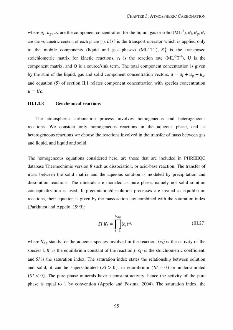
CHAPTER 3: ATMOSPHERIC CARBONATION
95
where , , are the component concentration for the liquid, gas or solid (ML-3
), , , are the volumetric content of each phase (-), is the transport operator which is applied only
to the mobile components (liquid and gas phases) (ML-3
T-1
), is the transposed
stoichiometric matrix for kinetic reactions, rk is the reaction rate (ML-3
T-1
), U is the
component matrix, and Q is a source/sink term. The total component concentration is given
by the sum of the liquid, gas and solid component concentration vectors, , and equation (5) of section II.1 relates component concentration with species concentration .
III.1.3.3 Geochemical reactions
The atmospheric carbonation process involves homogeneous and heterogeneous
reactions. We consider only homogeneous reactions in the aqueous phase, and as
heterogeneous reactions we choose the reactions involved in the transfer of mass between gas
and liquid, and liquid and solid.
The homogeneous equations considered here, are those that are included in PHREEQC
database Thermochimie version 8 such as dissociation, or acid-base reaction. The transfer of
mass between the solid matrix and the aqueous solution is modeled by precipitation and
dissolution reactions. The minerals are modeled as pure phase, namely not solid solution
conceptualization is used. If precipitation/dissolution processes are treated as equilibrium
reactions, their equation is given by the mass action law combined with the saturation index
(Parkhurst and Appelo, 1999):
(III.27)
where stands for the aqueous species involved in the reaction, is the activity of the
species , is the equilibrium constant of the reaction , is the stoichiometric coefficient,
and is the saturation index. The saturation index states the relationship between solution
and solid, it can be supersaturated ( ), in equilibrium ( ) or undersaturated . The pure phase minerals have a constant activity, hence the activity of the pure
phase is equal to 1 by convention (Appelo and Postma, 2004). The saturation index, the

CHAPTER 3: ATMOSPHERIC CARBONATION
96
logarithm of the quotient of the ion-activity product and the solubility constant, are set to zero,
in order to force equilibrium between the different mineral phases and the aqueous solution.
If a kinetic approach is chosen, the precipitation/dissolution processes are modeled by the
transition state theory which states that the reactants are in equilibrium with another species of
higher Gibbs free energy known as transition state complex. The rate equation is described by
(Lasaga et al., 1994):
, (III.28)
where is the rate, positive values represent dissolution processes and negatives precipitation
processes, is the kinetic constant, is the reactive surface per mass of water, is the
saturation index, and and are empirical parameters, and the subscript stand for the
reaction . The gas-liquid interactions are assumed to be in equilibrium and are modeled by the Henry's
law (Steefel et al., 2015):
, (III.29)
where is the fugacity of the gas species , is the Henry constant of the gas species , is the activity of the aqueous component , and the stoichiometric value of the gas species and the aqueous component . The fugacity is related to the partial pressure of the water by:
, (III.30)
where is the fugacity coefficient of the gas , and is the partial pressure of the gas . Ideal gases have a fugacity coefficient equal to 1, therefore its fugacity is equal to its partial
pressure. PHREEQC uses or ideal gases or gases under the Peng-Robinson model (Peng and
Robinson, 1976).

CHAPTER 3: ATMOSPHERIC CARBONATION
97
III.2 First modeling approach to the atmospheric carbonation problem
In this section we detail our first approaches to model the atmospheric carbonation
problem. We document the approach and expose some preliminary results.
III.2.1 Constant saturation test
III.2.1.1 Coupling procedure and hydraulic properties
In this test, it is assumed that all reactions are in equilibrium, there are no external
sink/source, saturation is constant, diffusion is the only transport mechanism, and the amount
of water released from the dissolution of hydrated products is ignored. The component mass
balance for a component in 1D is given by:
, (III.31)
where , , , , and are the volumetric content and component concentration for
liquid, gas and solid respectively. The diffusion values , and are calculated from the
Millington-Quirk equation (Millington, 1959):
, (III.32)
where is the effective diffusion of the component in the phase , is the molecular
diffusion coefficient of the component in the phase , is the porosity and is the
saturation of the phase , and are parameters specific to the material. The value of and for this experience are 2 and 4.2 (Richet et al., 2004; Thiery, 2006; Thiery et al., 2007).
We will use a sequential non-iterative approach. The transport step draws the spatial
discretization from the pdepe built-in function of MATLAB and integrates the spatial
discretization in time using a forward Euler method. Then, the new values of the aqueous
components and gas species (H2O ,CO2) are introduced in PHREEQC to obtain the new mass
balance between the different phases. The physical parameters for the problem are listed in
Table III-4.
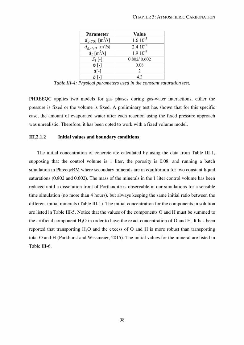
CHAPTER 3: ATMOSPHERIC CARBONATION
98
Parameter Value [m2/s] 1.6 10
-5 [m2/s] 2.4 10
-5 [m2/s] 1.9 10
-9 [-] 0.802/ 0.602 [-] 0.08 [-] 2 [-] 4.2
Table III-4: Physical parameters used in the constant saturation test.
PHREEQC applies two models for gas phases during gas-water interactions, either the
pressure is fixed or the volume is fixed. A preliminary test has shown that for this specific
case, the amount of evaporated water after each reaction using the fixed pressure approach
was unrealistic. Therefore, it has been opted to work with a fixed volume model.
III.2.1.2 Initial values and boundary conditions
The initial concentration of concrete are calculated by using the data from Table III-1,
supposing that the control volume is 1 liter, the porosity is 0.08, and running a batch
simulation in PhreeqcRM where secondary minerals are in equilibrium for two constant liquid
saturations (0.802 and 0.602). The mass of the minerals in the 1 liter control volume has been
reduced until a dissolution front of Portlandite is observable in our simulations for a sensible
time simulation (no more than 4 hours), but always keeping the same initial ratio between the
different initial minerals (Table III-1). The initial concentration for the components in solution
are listed in Table III-5. Notice that the values of the components O and H must be summed to
the artificial component H2O in order to have the exact concentration of O and H. It has been
reported that transporting H2O and the excess of O and H is more robust than transporting
total O and H (Parkhurst and Wissmeier, 2015). The initial values for the mineral are listed in
Table III-6.
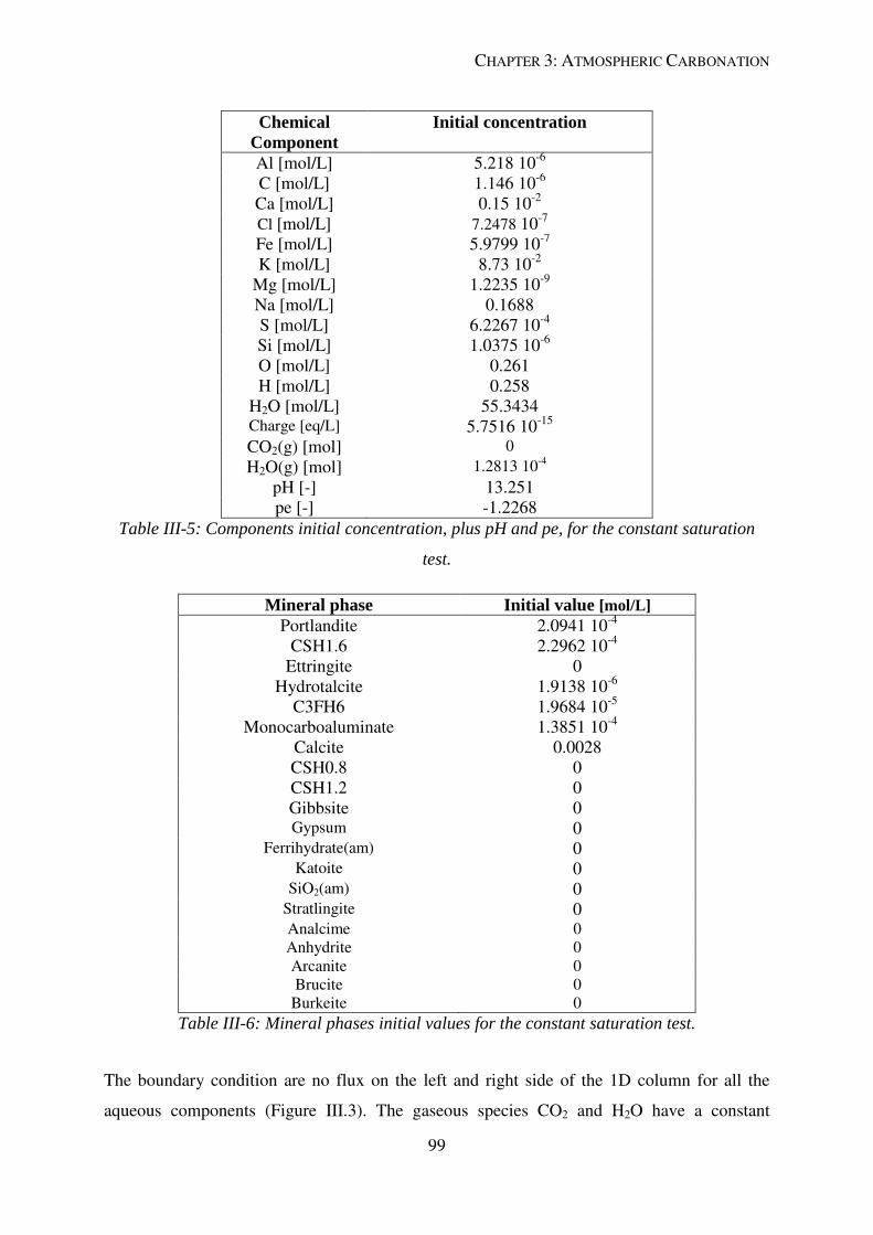
CHAPTER 3: ATMOSPHERIC CARBONATION
99
Chemical
Component
Initial concentration
Al [mol/L] 5.218 10-6
C [mol/L] 1.146 10-6
Ca [mol/L] 0.15 10-2
Cl [mol/L] 7.2478 10-7
Fe [mol/L] 5.9799 10-7
K [mol/L] 8.73 10-2
Mg [mol/L] 1.2235 10-9
Na [mol/L] 0.1688
S [mol/L] 6.2267 10-4
Si [mol/L] 1.0375 10-6
O [mol/L] 0.261
H [mol/L] 0.258
H2O [mol/L] 55.3434
Charge [eq/L] 5.7516 10-15
CO2(g) [mol] 0
H2O(g) [mol] 1.2813 10-4
pH [-] 13.251
pe [-] -1.2268
Table III-5: Components initial concentration, plus pH and pe, for the constant saturation
test.
Mineral phase Initial value [mol/L]
Portlandite 2.0941 10-4
CSH1.6 2.2962 10-4
Ettringite 0
Hydrotalcite 1.9138 10-6
C3FH6 1.9684 10-5
Monocarboaluminate 1.3851 10-4
Calcite 0.0028
CSH0.8 0
CSH1.2 0
Gibbsite 0
Gypsum 0 Ferrihydrate(am) 0
Katoite 0 SiO2(am) 0
Stratlingite 0 Analcime 0
Anhydrite 0
Arcanite 0
Brucite 0
Burkeite 0
Table III-6: Mineral phases initial values for the constant saturation test.
The boundary condition are no flux on the left and right side of the 1D column for all the
aqueous components (Figure III.3). The gaseous species CO2 and H2O have a constant
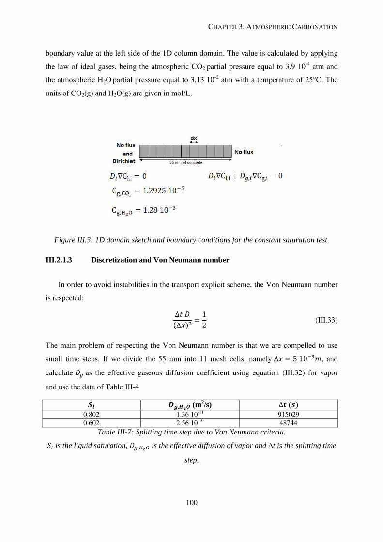
CHAPTER 3: ATMOSPHERIC CARBONATION
100
boundary value at the left side of the 1D column domain. The value is calculated by applying
the law of ideal gases, being the atmospheric CO2 partial pressure equal to 3.9 10-4
atm and
the atmospheric H2O partial pressure equal to 3.13 10-2
atm with a temperature of 25°C. The
units of CO2(g) and H2O(g) are given in mol/L.
Figure III.3: 1D domain sketch and boundary conditions for the constant saturation test.
III.2.1.3 Discretization and Von Neumann number
In order to avoid instabilities in the transport explicit scheme, the Von Neumann number
is respected:
(III.33)
The main problem of respecting the Von Neumann number is that we are compelled to use
small time steps. If we divide the 55 mm into 11 mesh cells, namely , and
calculate as the effective gaseous diffusion coefficient using equation (III.32) for vapor
and use the data of Table III-4 (m2/s)
0.802 1.36 10-11
915029
0.602 2.56 10-10
48744
Table III-7: Splitting time step due to Von Neumann criteria. is the liquid saturation, is the effective diffusion of vapor and ∆t is the splitting time
step.
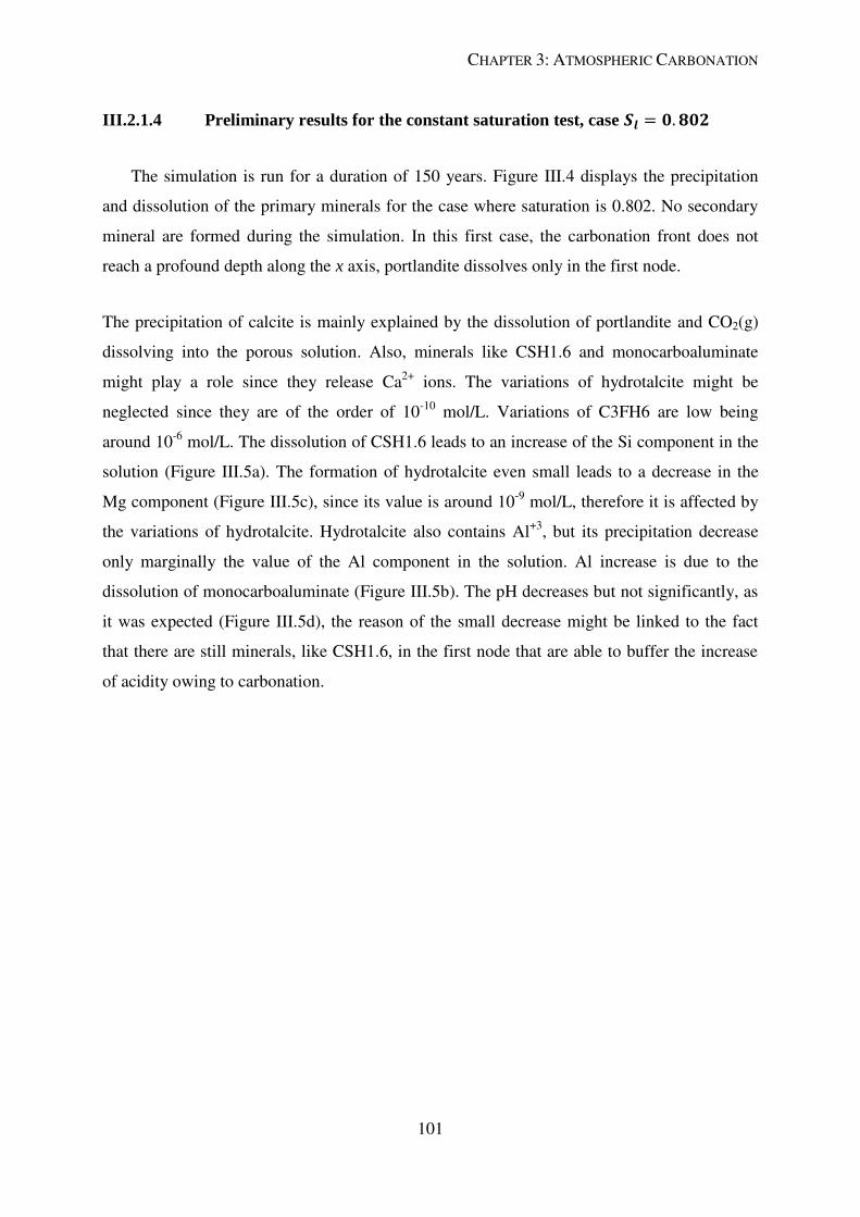
CHAPTER 3: ATMOSPHERIC CARBONATION
101
III.2.1.4 Preliminary results for the constant saturation test, case
The simulation is run for a duration of 150 years. Figure III.4 displays the precipitation
and dissolution of the primary minerals for the case where saturation is 0.802. No secondary
mineral are formed during the simulation. In this first case, the carbonation front does not
reach a profound depth along the x axis, portlandite dissolves only in the first node.
The precipitation of calcite is mainly explained by the dissolution of portlandite and CO2(g)
dissolving into the porous solution. Also, minerals like CSH1.6 and monocarboaluminate
might play a role since they release Ca2+
ions. The variations of hydrotalcite might be
neglected since they are of the order of 10-10
mol/L. Variations of C3FH6 are low being
around 10-6
mol/L. The dissolution of CSH1.6 leads to an increase of the Si component in the
solution (Figure III.5a). The formation of hydrotalcite even small leads to a decrease in the
Mg component (Figure III.5c), since its value is around 10-9
mol/L, therefore it is affected by
the variations of hydrotalcite. Hydrotalcite also contains Al+3
, but its precipitation decrease
only marginally the value of the Al component in the solution. Al increase is due to the
dissolution of monocarboaluminate (Figure III.5b). The pH decreases but not significantly, as
it was expected (Figure III.5d), the reason of the small decrease might be linked to the fact
that there are still minerals, like CSH1.6, in the first node that are able to buffer the increase
of acidity owing to carbonation.
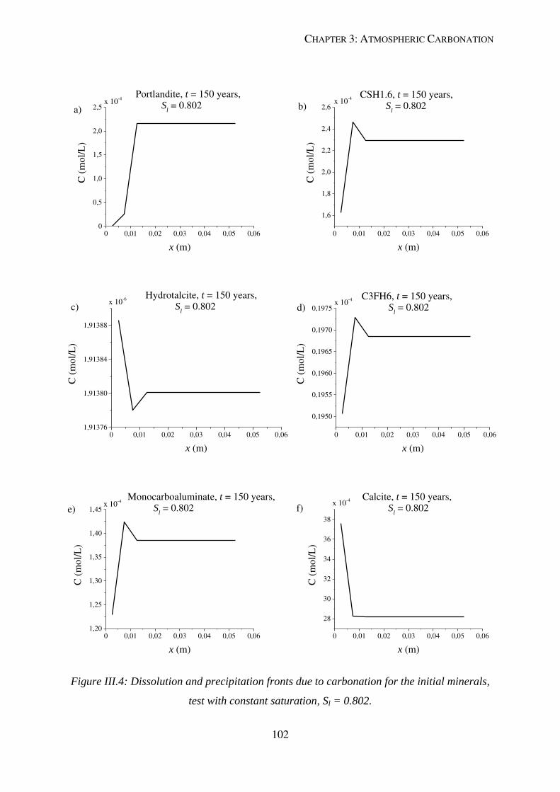
CHAPTER 3: ATMOSPHERIC CARBONATION
102
0,01 0,02 0,03 0,04 0,05 0,060
0,5
1,0
1,5
2,0
2,5
0
Sl = 0.802
C (
mol/
L)
x (m)
Portlandite, t = 150 years,x 10
-4
a)
0,01 0,02 0,03 0,04 0,05 0,060
1,6
1,8
2,0
2,2
2,4
2,6b)x 10
-4
C (
mol/
L)
x (m)
Sl = 0.802
CSH1.6, t = 150 years,
0,01 0,02 0,03 0,04 0,05 0,0601,91376
1,91380
1,91384
1,91388
C (
mol/
L)
x (m)
Sl = 0.802
Hydrotalcite, t = 150 years,x 10
-6
c)
0,01 0,02 0,03 0,04 0,05 0,060
0,1950
0,1955
0,1960
0,1965
0,1970
0,1975C
(m
ol/
L)
x (m)
Sl = 0.802
C3FH6, t = 150 years,x 10
-4
d)
0,01 0,02 0,03 0,04 0,05 0,0601,20
1,25
1,30
1,35
1,40
1,45
C (
mo
l/L
)
x (m)
x 10-4
e) Sl = 0.802
Monocarboaluminate, t = 150 years,
0,01 0,02 0,03 0,04 0,05 0,060
28
30
32
34
36
38
C (
mo
l/L
)
x (m)
x 10-4
f) Sl = 0.802
Calcite, t = 150 years,
Figure III.4: Dissolution and precipitation fronts due to carbonation for the initial minerals,
test with constant saturation, Sl = 0.802.
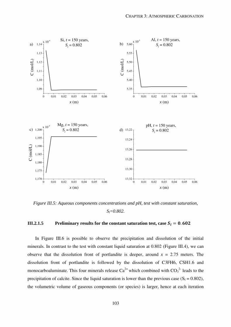
CHAPTER 3: ATMOSPHERIC CARBONATION
103
0,01 0,02 0,03 0,04 0,05 0,060
1,09
1,10
1,11
1,12
1,13
1,14
C (
mol/
L)
x (m)
x 10-4
a) Sl = 0.802
Si, t = 150 years,
0,01 0,02 0,03 0,04 0,05 0,060
5,35
5,40
5,45
5,50
5,55
5,60
C (
mol/
L)
x (m)
Sl = 0.802
Al, t = 150 years,x 10
-5
b)
0,01 0,02 0,03 0,04 0,05 0,0601,170
1,175
1,180
1,185
1,190
1,195
1,200
C (
mol/
L)
x (m)
Sl = 0.802
Mg, t = 150 years,c)
x 10-9
0,01 0,02 0,03 0,04 0,05 0,06013,32
13,30
13,28
13,26
13,24
13,22d)
x (m)
Sl = 0.802
pH, t = 150 years,
Figure III.5: Aqueous components concentrations and pH, test with constant saturation,
Sl=0.802.
III.2.1.5 Preliminary results for the constant saturation test, case
In Figure III.6 is possible to observe the precipitation and dissolution of the initial
minerals. In contrast to the test with constant liquid saturation at 0.802 (Figure III.4), we can
observe that the dissolution front of portlandite is deeper, around x = 2.75 meters. The
dissolution front of portlandite is followed by the dissolution of C3FH6, CSH1.6 and
monocarboaluminate. This four minerals release Ca2+
which combined with CO32-
leads to the
precipitation of calcite. Since the liquid saturation is lower than the previous case (Sl = 0.802),
the volumetric volume of gaseous components (or species) is larger, hence at each iteration
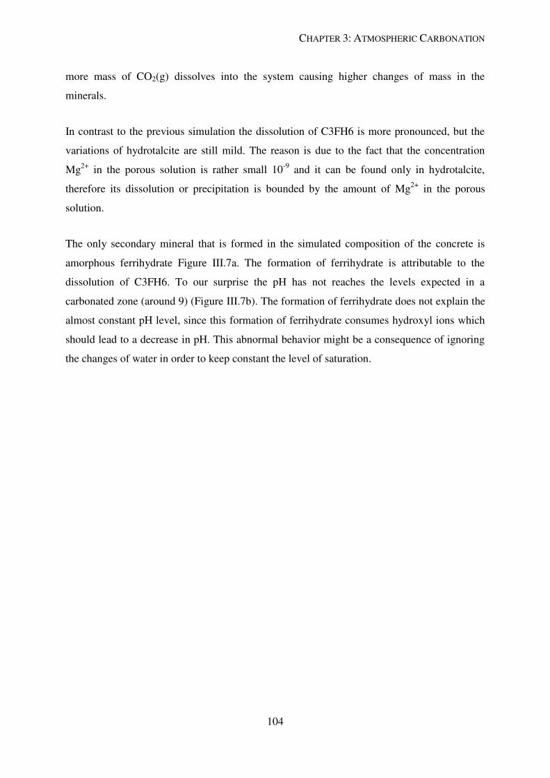
CHAPTER 3: ATMOSPHERIC CARBONATION
104
more mass of CO2(g) dissolves into the system causing higher changes of mass in the
minerals.
In contrast to the previous simulation the dissolution of C3FH6 is more pronounced, but the
variations of hydrotalcite are still mild. The reason is due to the fact that the concentration
Mg2+
in the porous solution is rather small 10-9
and it can be found only in hydrotalcite,
therefore its dissolution or precipitation is bounded by the amount of Mg2+
in the porous
solution.
The only secondary mineral that is formed in the simulated composition of the concrete is
amorphous ferrihydrate Figure III.7a. The formation of ferrihydrate is attributable to the
dissolution of C3FH6. To our surprise the pH has not reaches the levels expected in a
carbonated zone (around 9) (Figure III.7b). The formation of ferrihydrate does not explain the
almost constant pH level, since this formation of ferrihydrate consumes hydroxyl ions which
should lead to a decrease in pH. This abnormal behavior might be a consequence of ignoring
the changes of water in order to keep constant the level of saturation.
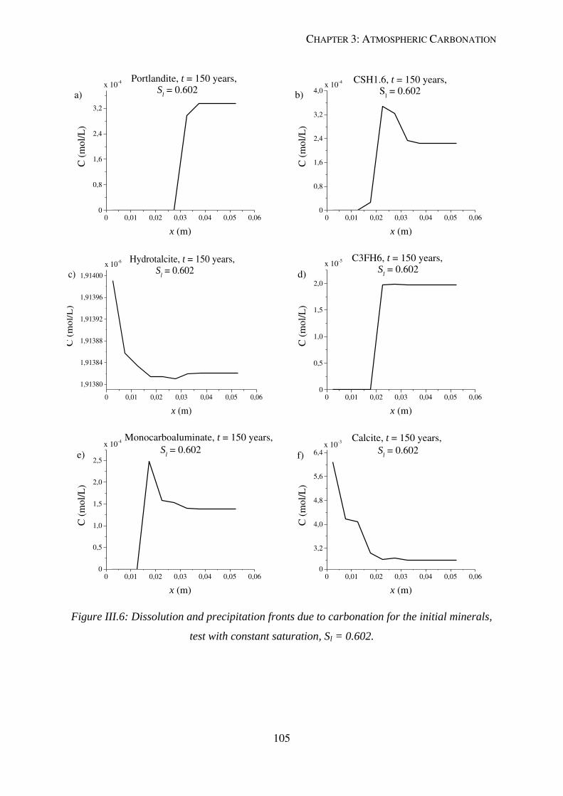
CHAPTER 3: ATMOSPHERIC CARBONATION
105
0,01 0,02 0,03 0,04 0,05 0,060
0,8
1,6
2,4
3,2
0
C (
mol/
L)
x (m)
a)x 10
-4 Portlandite, t = 150 years,S
l = 0.602
0,01 0,02 0,03 0,04 0,05 0,060
0,8
1,6
2,4
3,2
4,0
0
C (
mol/
L)
x (m)
CSH1.6, t = 150 years,S
l = 0.602
x 10-4
b)
0,01 0,02 0,03 0,04 0,05 0,060
1,91380
1,91384
1,91388
1,91392
1,91396
1,91400
C (
mo
l/L
)
x (m)
Hydrotalcite, t = 150 years,S
l = 0.602c)
x 10-6
0,01 0,02 0,03 0,04 0,05 0,060
0,5
1,0
1,5
2,0
0
C (
mol/
L)
x (m)
Sl = 0.602
C3FH6, t = 150 years,x 10
-5
d)
0,01 0,02 0,03 0,04 0,05 0,060
0,5
1,0
1,5
2,0
2,5
0
C (
mol/
L)
x (m)
Monocarboaluminate, t = 150 years,
Sl = 0.602
e)x 10
-4
0,01 0,02 0,03 0,04 0,05 0,060
3,2
4,0
4,8
5,6
6,4
0
C (
mol/
L)
x (m)
Calcite, t = 150 years,
Sl = 0.602
f)x 10
-3
Figure III.6: Dissolution and precipitation fronts due to carbonation for the initial minerals,
test with constant saturation, Sl = 0.602.
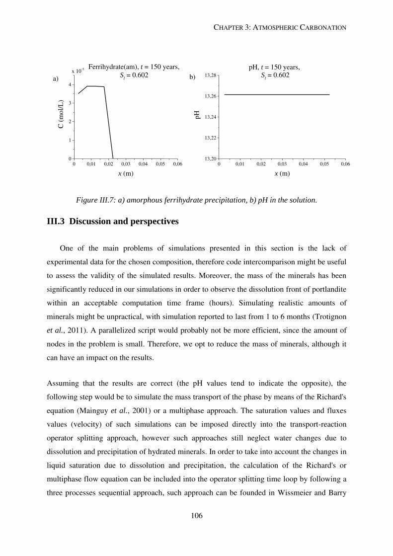
CHAPTER 3: ATMOSPHERIC CARBONATION
106
0,01 0,02 0,03 0,04 0,05 0,060
1
2
3
4
0
C (
mol/
L)
x (m)
Sl = 0.602
Ferrihydrate(am), t = 150 years,
a)x 10
-5
0,01 0,02 0,03 0,04 0,05 0,06013,20
13,22
13,24
13,26
13,28b)
pH
x (m)
pH, t = 150 years,S
l = 0.602
Figure III.7: a) amorphous ferrihydrate precipitation, b) pH in the solution.
III.3 Discussion and perspectives
One of the main problems of simulations presented in this section is the lack of
experimental data for the chosen composition, therefore code intercomparison might be useful
to assess the validity of the simulated results. Moreover, the mass of the minerals has been
significantly reduced in our simulations in order to observe the dissolution front of portlandite
within an acceptable computation time frame (hours). Simulating realistic amounts of
minerals might be unpractical, with simulation reported to last from 1 to 6 months (Trotignon
et al., 2011). A parallelized script would probably not be more efficient, since the amount of
nodes in the problem is small. Therefore, we opt to reduce the mass of minerals, although it
can have an impact on the results.
Assuming that the results are correct (the pH values tend to indicate the opposite), the
following step would be to simulate the mass transport of the phase by means of the Richard's
equation (Mainguy et al., 2001) or a multiphase approach. The saturation values and fluxes
values (velocity) of such simulations can be imposed directly into the transport-reaction
operator splitting approach, however such approaches still neglect water changes due to
dissolution and precipitation of hydrated minerals. In order to take into account the changes in
liquid saturation due to dissolution and precipitation, the calculation of the Richard's or
multiphase flow equation can be included into the operator splitting time loop by following a
three processes sequential approach, such approach can be founded in Wissmeier and Barry
CHAPTER 3: ATMOSPHERIC CARBONATION
107
(2011). This property update is considered as evaluated in lagged time (Nardi et al., 2014),
and in decoupled processes software it is not only applicable to water changes due to
chemistry, but also porosity changes (Radu et al., 2013). In principle, such approach is
considered to be applicable when changes are not significant, but the numerical error
introduced by such approaches is unclear. The application of Taylor series for simple
chemistry systems on the H2O component might be helpful.
Therefore, if accuracy and separation of processes are desired, a fixed-point iteration
approach has to be used. It is considered that a two fixed-point iterations should be applied,
one for transport and flow, and the other for the first coupling (transport+flow) and the
reaction operator. If PHREEQC software is used, a new implementation for the iterative
approach must be considered. iPhreeqc does not allow to copy iPhreeqc objects into new
variables, but the exact amount of each component, minerals and other chemical entities can
be dumped into an external file, which can be reused later to see invariant values of the
iterative process. We do not know the consequences of using two fixed-point iteration
approaches, but we hypothesize that the already existing convergence and performance time
problems of iterative approaches might be enhanced in a case where two fixed-point iteration
methods are used.
Another weak point of our simulation is assuming that all aqueous species have the same
diffusion-dispersion coefficient. Since we are not dealing with advection-dominanted
transport, such approach is not less realistic but it is functional for first approaches, giving an
understanding of the evolution of the system. Different values of the diffusion coefficient can
also imply a contribution in the operator splitting error, as seen in section II.4.2.

108
CHAPTER 4: CONCLUSION
109
IV CONCLUSION
This thesis explores the application of operator splitting approaches in the field of reactive
transport modeling, aiming to solve each part of the decoupled problem with a suitable solver,
and to apply the developed work into the atmospheric carbonation problematic which arises in
the storage concrete packages of intermediate-level long-lived waste of a nuclear repository.
An object-oriented programming paradigm has been used to develop a fully segmented
implementation of a general expression of the operator splitting approaches. The
object-oriented paradigm has provided a satisfactory set of characteristics such as
encapsulation of data and methods, reusability, and extensibility. Other works in reactive
transport modeling have acknowledged the advantages of such programming paradigm
(Gamazo et al., 2016; Kolditz and Bauer, 2004). We also underline that although we work
only with transport and chemical operators the generic approach used here allows to separate
the operators in different processes, e.g. advection-reaction and diffusion (Liu and Ewing,
2005) and to implement easily other methods such as the one presented in Gasda et al. (2011).
Amongst the generic operator splitting approaches that have been implemented into the
present code named TReacLab, it is possible to find sequential, additive, alternating, Strang,
and symmetrically weighted splitting methods (Csomós and Faragó, 2008; Faragó et al.,
2008; Simpson et al., 2005; Strang, 1968). Furthermore, a fixed-point (or Picard iteration)
approach for two classical formulations in the field of reactive transport have been
implemented: SIA CC, and SIA TC (de Dieuleveult et al., 2009). It has been corroborated by
the applied practical cases that all the operator splitting approaches are consistent and valid.
Moreover, if we consider well-posed PDEs with a consistent decomposition of each operator
which are accurate enough and stable, we should expect better results using second-order
accurate operator splitting approaches. The iterative approaches have not been able to reach
convergence in all the cases which makes us rethink about how general our iterative
implementation is, since initially it was crafted to work only for cases dealing with speciation
and precipitation/dissolution at equilibrium.
The operators splitting introduces an error associated with the separation of processes
(Valocchi and Malmstead, 1992). The error has usually been limited to single species (Barry
et al., 1996) and sometimes have been understood heuristically (Jacques et al., 2006). In order
CHAPTER 4: CONCLUSION
110
to understand better the error, which might help to understand results and better design
operator splitting approaches, the temporal truncation error is studied. If only chemical
kinetics equations are considered, it is possible to assess the error for each species or
component by means of Taylor series (Csomós and Faragó, 2008; Csomós et al., 2005;
Simpson and Landman, 2008) or Lie formalism (Lanser and Verwer, 1999). These
calculations can be tedious, therefore symbolic computation might play a role in order to
identify the sources of error.
Several external transport solvers (COMSOL, pdepe MATLAB, FVTool, and FD scripts) and
geochemical codes (iPhreeqc, PhreeqcRM) have been plugged with good results. The
combination of the external codes with the operator splitting methodes (iterative and
non-iterative) must be always assessed. For instance, solvers that use first-order time
integration scheme might cause a reduction in the order of the truncation error when they are
combined with a second-order operator splitting such as Strang method (Csomós and Faragó,
2008). Also, some implemented algorithms work only with implicit or explicit schemes, such
as the SIA CC. Moreover, we have notice that COMSOL suffers from a time penalization
each time that is called from MATLAB. That fact makes COMSOL, not the best tool for
problems with a low number of grids. Although, COMSOL performs better than other
software. The use of black boxes for research is questionable, black boxes might be a problem
when transparence is search.
The carbonation simulations are not mature enough to draw general conclusions. The main
problem currently faced is to find acceptable concrete mineral compositions that can be
simulated in a reasonable time. Additionally, we notice that if we want to take into account
the influence of mineral dissolution into the flow process an iterative approach must be
implemented. Comparison of non-iterative approaches against the iterative approach can show
how relevant is the mineral dissolution into the flow process.

CHAPTER 4: CONCLUSION
111
112
REFERENCES
Abriola, L.M., Pinder, G.F., 1985. A Multiphase Approach to the Modeling of Porous Media
Contamination by Organic Compounds: 1. Equation Development. Water Resources
Research 21, 11-18.
Amir, L., Kern, M., 2010. A global method for coupling transport with chemistry in
heterogeneous porous media. Computational Geosciences 14, 465-481.
Amos, R.T., Mayer, K.U., Blowes, D.W., Ptacek, C.J., 2004. Reactive Transport Modeling of
Column Experiments for the Remediation of Acid Mine Drainage. Environmental
Science & Technology 38, 3131-3138.
ANDRA, D., 2005a. Andra Research on the Geological Disposal of Highlevel Long-lived
Radioactive Waste–Results and Perspectives, Chatenay-Malabry, France., p. 40.
ANDRA, S.A., 2005b. Evaluation of the feasibility of a geological repository in an
argillaceous formation. Andra, Chatenay-Malabry, France.
Appelo, C., Rolle, M., 2010. PHT3D: A reactive multicomponent transport model for
saturated porous media. Groundwater 48, 627-632.
Appelo, C.A.J., Postma, D., 2004. Geochemistry, groundwater and pollution. CRC press.
ASN, 2008. Guide de sûreté relatif au stockage définitif des déchets radioactifs en formation
géologique profonde, 32 p.
Barrodale, I., Roberts, F.D.K., 1978. An Efficient Algorithm for Discrete L1 Linear
Approximation with Linear Constraints. SIAM Journal on Numerical Analysis 15,
603-611.
Barrodale, I., Roberts, F.D.K., 1980. Algorithm 552: Solution of the Constrained L1 Linear
Approximation Problem. ACM Trans. Math. Softw. 6, 231-235.
Barry, D.A., Miller, C.T., Culligan-Hensley, P.J., 1996. Temporal discretisation errors in non-
iterative split-operator approaches to solving chemical reaction/groundwater transport
models. Journal of Contaminant Hydrology 22, 1-17.
Bary, B., Mügler, C., 2006. Simplified modelling and numerical simulations of concrete
carbonation in unsaturated conditions. Revue européenne de génie civil 10, 1049-
1072.
Bary, B., Sellier, A., 2004. Coupled moisture—carbon dioxide–calcium transfer model for
carbonation of concrete. Cement and Concrete Research 34, 1859-1872.

113
Bastian, P., 1999. Numerical computation of multiphase flows in porous media.
habilitationsschrift Univeristät Kiel.
Bear, J., 1972. Dynamics of fluids in porous media. Elsevier, New York.
Besnard, K., 2004. Modélisation du transport réactif dans les milieux poreux hétérogènes.
Application aux processus d'adsorption cinétique non linéaire, Geosciences Rennes.
Universite de Rennes I, France.
Beven, K., Germann, P., 2013. Macropores and water flow in soils revisited. Water Resources
Research 49, 3071-3092.
Bjerrum, N., 1926. I. Influence of ionic association on the activity of ions at moderate degrees
of association. K. Dan. Vidensk. Selsk 7, 1-48.
Bozau, E., van Berk, W., 2013. Hydrogeochemical Modeling of Deep Formation Water
Applied to Geothermal Energy Production. Procedia Earth and Planetary Science 7,
97-100.
Brinkley , S.R., 1947. Calculation of the equilibrium composition of systems of many
constituents. The Journal of Chemical Physics 15, 107-110.
Brooks, R.H., Corey, A.T., 1964. Hydraulic Properties of Porous Media. Colorado State
University.
Bullard, J.W., Jennings, H.M., Livingston, R.A., Nonat, A., Scherer, G.W., Schweitzer, J.S.,
Scrivener, K.L., Thomas, J.J., 2011. Mechanisms of cement hydration. Cement and
Concrete Research 41, 1208-1223.
Burnett, R.D., Frind, E.O., 1987. Simulation of contaminant transport in three dimensions: 2.
Dimensionality effects. Water Resources Research 23, 695-705.
Carrayrou, J., Hoffmann, J., Knabner, P., Kräutle, S., de Dieuleveult, C., Erhel, J., Van der
Lee, J., Lagneau, V., Mayer, K.U., MacQuarrie, K.T.B., 2010. Comparison of
numerical methods for simulating strongly nonlinear and heterogeneous reactive
transport problems—the MoMaS benchmark case. Computational Geosciences 14,
483-502.
Carrayrou, J., Mosé, R., Behra, P., 2004. Operator-splitting procedures for reactive transport
and comparison of mass balance errors. Journal of Contaminant Hydrology 68, 239-
268.
Charlton, S.R., Parkhurst, D.L., 2011. Modules based on the geochemical model PHREEQC
for use in scripting and programming languages. Computers & Geosciences 37, 1653-
1663.

114
Chen, X., Thornton, S.F., Small, J., 2015. Influence of Hyper-Alkaline pH Leachate on
Mineral and Porosity Evolution in the Chemically Disturbed Zone Developed in the
Near-Field Host Rock for a Nuclear Waste Repository. Transport in Porous Media
107, 489-505.
Chen, Z., Ewing, R., Espedal, M., 1994. Multiphase flow simulation with various boundary
conditions. Computational Methods in Water Resources, 925-932.
Cho, C., 1971. Convective transport of ammonium with nitrification in soil. Canadian Journal
of Soil Science 51, 339-350.
Clement, T.P., Sun, Y., Hooker, B.S., Petersen, J.N., 1998. Modeling Multispecies Reactive
Transport in Ground Water. Ground Water Monitoring & Remediation 18, 79-92.
Cochepin, B., Trotignon, L., Bildstein, O., Steefel, C.I., Lagneau, V., Van der lee, J., 2008.
Approaches to modelling coupled flow and reaction in a 2D cementation experiment.
Advances in Water Resources 31, 1540-1551.
COMSOL, A., 2010. COMSOL Multiphysics-LiveLink for Matlab User’s Guide, comsol 4.1 edition.
COMSOL, A., 2012. 4.3 User’s Guide. Comsol.
Corey, A.T., 1954. The interrelation between gas and oil relative permeabilities. Producers
monthly 19, 38-41.
Csomós, P., Faragó, I., 2008. Error analysis of the numerical solution of split differential
equations. Mathematical and Computer Modelling 48, 1090-1106.
Csomós, P., Faragó, I., Havasi, Á., 2005. Weighted sequential splittings and their analysis.
Computers & Mathematics with Applications 50, 1017-1031.
Darcy, H., 1856. Les fontaines publiques de la ville de Dijon: exposition et application. Victor
Dalmont.
de Dieuleveult, C., Erhel, J., 2010. A global approach to reactive transport: application to the
MoMas benchmark. Computational Geosciences 14, 451-464.
de Dieuleveult, C., Erhel, J., Kern, M., 2009. A global strategy for solving reactive transport
equations. Journal of Computational Physics 228, 6395-6410.
de Sousa, E.R., 2012. Groundwater modelling meets geochemistry: Building the bridge
between FEFLOW and PHREEQC with IFMPhreeqc, In: Association, I.M.W. (Ed.),
Annual Conference.
115
Debure, M., De Windt, L., Frugier, P., Gin, S., 2013. HLW glass dissolution in the presence
of magnesium carbonate: Diffusion cell experiment and coupled modeling of diffusion
and geochemical interactions. Journal of Nuclear Materials 443, 507-521.
Dentz, M., Le Borgne, T., Englert, A., Bijeljic, B., 2011. Mixing, spreading and reaction in
heterogeneous media: A brief review. Journal of Contaminant Hydrology 120, 1-17.
Dittrich, T.M., Reimus, P.W., 2015. Uranium transport in a crushed granodiorite:
Experiments and reactive transport modeling. Journal of Contaminant Hydrology 175–176, 44-59.
Dobson, P.F., Kneafsey, T.J., Sonnenthal, E.L., Spycher, N., Apps, J.A., 2003. Experimental
and numerical simulation of dissolution and precipitation: implications for fracture
sealing at Yucca Mountain, Nevada. Journal of Contaminant Hydrology 62–63, 459-
476.
Douglas, J., Jr., Peaceman, D.W., Rachford, H.H., Jr., 1959. A Method for Calculating Multi-
Dimensional Immiscible Displacement. Society of Petroleum Engineers.
Duprat, F., Vu, N.T., Sellier, A., 2014. Accelerated carbonation tests for the probabilistic
prediction of the durability of concrete structures. Construction and Building Materials
66, 597-605.
Dupuis, M.-C., Gonnot, F.-M., 2013. The Cigeo project: Meuse/Haute-Marne reversible
geological disposal facility for radioactive waste. Andra, Chatenay-Malabry, France.,
p. 104.
Eftekhari, A.A., 2016. https://zenodo.org/record/18156#.WK63llXhCUk.
Ekolu, S.O., 2016. A review on effects of curing, sheltering, and CO2 concentration upon
natural carbonation of concrete. Construction and Building Materials 127, 306-320.
Engesgaard, P., Kipp, K.L., 1992. A geochemical transport model for redox-controlled
movement of mineral fronts in groundwater flow systems: A case of nitrate removal
by oxidation of pyrite. Water Resources Research 28, 2829-2843.
Ewing, R.E., 1991. Simulation of multiphase flows in porous media, Mathematical Modeling
for Flow and Transport Through Porous Media. Springer, pp. 479-499.
Fahs, M., Carrayrou, J., Younes, A., Ackerer, P., 2008. On the Efficiency of the Direct
Substitution Approach for Reactive Transport Problems in Porous Media. Water, Air,
and Soil Pollution 193, 299-308.
Faragó, I., Gnandt, B., Havasi, Á., 2008a. Additive and iterative operator splitting methods
and their numerical investigation. Computers & Mathematics with Applications 55,
2266-2279.

116
Farago, I., Havasi, A., 2005. On the convergence and local splitting error of different splitting
schemes. Progress in Computational Fluid Dynamics, an International Journal 5, 495-
504.
Faragó, I., Thomsen, P.G., Zlatev, Z., 2008b. On the additive splitting procedures and their
computer realization. Applied Mathematical Modelling 32, 1552-1569.
Fick, A., 1855. V. On liquid diffusion. The London, Edinburgh, and Dublin Philosophical
Magazine and Journal of Science 10, 30-39.
Florez, W.F., Portapila, M., Hill, A.F., Power, H., Orsini, P., Bustamante, C.A., 2015. The
control volume radial basis function method CV-RBF with Richardson extrapolation
in geochemical problems. Computers & Geosciences 76, 151-163.
Frippiat, C.C., Holeyman, A.E., 2008. A comparative review of upscaling methods for solute
transport in heterogeneous porous media. Journal of Hydrology 362, 150-176.
Gamazo, P., Slooten, L.J., Carrera, J., Saaltink, M.W., Bea, S., Soler, J., 2016. PROOST:
object-oriented approach to multiphase reactive transport modeling in porous media.
Journal of Hydroinformatics 18, 310-328.
Gasda, S.E., Farthing, M.W., Kees, C.E., Miller, C.T., 2011. Adaptive split-operator methods
for modeling transport phenomena in porous medium systems. Advances in Water
Resources 34, 1268-1282.
Geiser, J., 2009. Decomposition methods for differential equations: theory and applications.
CRC Press.
Gerke, H.H., van Genuchten, M.T., 1993. A dual-porosity model for simulating the
preferential movement of water and solutes in structured porous media. Water
Resources Research 29, 305-319.
Glasser, F.P., Marchand, J., Samson, E., 2008. Durability of concrete — Degradation
phenomena involving detrimental chemical reactions. Cement and Concrete Research
38, 226-246.
Glenn, H., Peter, L., Chuan, L., 2007. Subsurface multiphase flow and multicomponent
reactive transport modeling using high-performance computing. Journal of Physics:
Conference Series 78, 012025.
Gramling, C.M., Harvey, C.F., Meigs, L.C., 2002. Reactive transport in porous media: A
comparison of model prediction with laboratory visualization. Environmental Science
& Technology 36, 2508-2514.
Hammond, G.E., Valocchi, A.J., Lichtner, P.C., 2005. Application of Jacobian-free Newton–Krylov with physics-based preconditioning to biogeochemical transport. Advances in
Water Resources 28, 359-376.

117
Hassan, A.E., 2004. Validation of numerical ground water models used to guide decision
making. Ground Water 42, 277-290.
Hassanizadeh, S.M., Celia, M.A., Dahle, H.K., 2002. Dynamic effect in the capillary
pressure–saturation relationship and its impacts on unsaturated flow. Vadose Zone
Journal 1, 38-57.
He, W., Beyer, C., Fleckenstein, J.H., Jang, E., Kolditz, O., Naumov, D., Kalbacher, T., 2015.
A parallelization scheme to simulate reactive transport in the subsurface environment
with OGS#IPhreeqc 5.5.7-3.1.2. Geosci. Model Dev. 8, 3333-3348.
Hoffmann, J., Kräutle, S., Knabner, P., 2010. A parallel global-implicit 2-D solver for reactive
transport problems in porous media based on a reduction scheme and its application to
the MoMaS benchmark problem. Computational Geosciences 14, 421-433.
Hoffmann, J., Kräutle, S., Knabner, P., 2012. A general reduction scheme for reactive
transport in porous media. Computational Geosciences 16, 1081-1099.
Holden, H., Karlsen, K.H., Lie, K.-A., Risebro, N.H., 2010. Splitting methods for partial
differential equations with rough solutions: Analysis and MATLAB programs.
European Mathematical Society.
Hoth, N., Kornjaev, A., Hafner, F., 2000. Reactive transport modelling with simulator
MODCALIF-CHEM: prediction of the environmental impact of lignite dump waters.
IAHS PUBLICATION, 481-488.
Hubbert, M.K., 1957. Darcy's law and the field equations of the flow of underground fluids.
Hydrological Sciences Journal 2, 23-59.
Huber, P., Nivelon, S., Ottenio, P., Nortier, P., 2013. Coupling a Chemical Reaction Engine
with a Mass Flow Balance Process Simulation for Scaling Management in
Papermaking Process Waters. Industrial & Engineering Chemistry Research 52, 421-
429.
Hundsdorfer, W., Verwer, J.G., 2013. Numerical solution of time-dependent advection-
diffusion-reaction equations. Springer Science & Business Media.
Jacques, D., Šimůnek, J., 2005. User manual of the multicomponent variably-saturated flow
and transport model HP1. Description, Verification and Examples, Version 1, 79.
Jacques, D., Šimůnek, J., Mallants, D., Van Genuchten, M.T., 2006. Operator-splitting errors
in coupled reactive transport codes for transient variably saturated flow and
contaminant transport in layered soil profiles. Journal of Contaminant Hydrology 88,
197-218.
Jensen, M.M., 2014. A Coupled Transport and Chemical Model for Durability Predictions of
Cement Based Materials. Technical University of DenmarkDanmarks Tekniske
118
Universitet, Department of Structural Engineering and MaterialsInstitut for Bærende
Konstruktioner og Materialer.
Jensen, M.M., Johannesson, B., Geiker, M.R., 2014. Framework for reactive mass transport:
Phase change modeling of concrete by a coupled mass transport and chemical
equilibrium model. Computational Materials Science 92, 213-223.
Kaluarachchi, J.J., Morshed, J., 1995. Critical assessment of the operator-splitting technique
in solving the advection-dispersion-reaction equation: 1. First-order reaction.
Advances in Water Resources 18, 89-100.
Kazemi Nia Korrani, A., Jerauld, G.R., Sepehrnoori, K., 2016a. Mechanistic Modeling of
Low-Salinity Waterflooding Through Coupling a Geochemical Package With a
Compositional Reservoir Simulator. SPE Reservoir Evaluation & Engineering.
Kazemi Nia Korrani, A., Sepehrnoori, K., Delshad, M., 2015. Coupling IPhreeqc with
UTCHEM to model reactive flow and transport. Computers & Geosciences 82, 152-
169.
Kazemi Nia Korrani, A., Sepehrnoori, K., Delshad, M., 2016b. A Mechanistic Integrated
Geochemical and Chemical-Flooding Tool for Alkaline/Surfactant/Polymer Floods.
SPE Journal 21, 32-54.
Kolditz, O., Bauer, S., 2004. A process-oriented approach to computing multi-field problems
in porous media. Journal of Hydroinformatics 6, 225-244.
Kolditz, O., Bauer, S., Bilke, L., Böttcher, N., Delfs, J.-O., Fischer, T., Görke, U.J.,
Kalbacher, T., Kosakowski, G., McDermott, C., 2012. OpenGeoSys: an open-source
initiative for numerical simulation of thermo-hydro-mechanical/chemical (THM/C)
processes in porous media. Environmental Earth Sciences 67, 589-599.
Koren, B., 1993. A robust upwind discretization method for advection, diffusion and source
terms. Centrum voor Wiskunde en Informatica Amsterdam.
Kulik, D.A., 2011. Improving the structural consistency of C-S-H solid solution
thermodynamic models. Cement and Concrete Research 41, 477-495.
Kumar, D., Kumar, V., Singh, V.P., 2010. Mathematical modeling of brown stock washing
problems and their numerical solution using MATLAB. Computers & Chemical
Engineering 34, 9-16.
Langergraber, G., Šimůnek, J., 2012. Reactive transport modeling of subsurface flow constructed wetlands using the HYDRUS wetland module. Vadose Zone Journal 11.
Lanser, D., Verwer, J.G., 1999. Analysis of operator splitting for advection–diffusion–reaction problems from air pollution modelling. Journal of Computational and Applied
Mathematics 111, 201-216.

119
Lapidus, L., Amundson, N.R., 1952. Mathematics of adsorption in beds. VI. The effect of
longitudinal diffusion in ion exchange and chromatographic columns. The Journal of
Physical Chemistry 56, 984-988.
Lasaga, A.C., Soler, J.M., Ganor, J., Burch, T.E., Nagy, K.L., 1994. Chemical weathering rate
laws and global geochemical cycles. Geochimica et Cosmochimica Acta 58, 2361-
2386.
Lee, J.H., Siegel, M.D., Arguello Jr, J.G., Webb, S.W., Dewers, T.A., Mariner, P.E., Edwards,
H.C., Fuller, T.J., Freeze, G.A., Jove-Colon, C.F., 2011. Nuclear Energy Advanced
Modeling and Simulation (NEAMS) waste Integrated Performance and Safety Codes
(IPSC): gap analysis for high fidelity and performance assessment code development.
Sandia National Laboratories.
Lichtner , P.C., Hammond, G.E., Lu, C., Karra, S., Bisht, G., Andre, B., Mills, R., Kumar, J.,
2015. PFLOTRAN User Manual.
Lie, K., 2014. An introduction to reservoir simulation using MATLAB: User guide for the
Matlab reservoir simulation toolbox (MRST), SINTEF ICT, Department of Applied
Mathematics, Oslo, Norway.
Likos, W.J., Lu, N., 2004. Hysteresis of capillary stress in unsaturated granular soil. Journal
of engineering mechanics 130, 646-655.
Liu, J., Ewing, R.E., 2005. An operator splitting method for nonlinear reactive transport
equations and its implementation based on dll and com, Current Trends in High
Performance Computing and Its Applications. Springer, pp. 93-102.
Lunn, M., Lunn, R.J., Mackayb, R., 1996. Determining analytic solutions of multiple species
contaminant transport, with sorption and decay. Journal of Hydrology 180, 195-210.
Mainguy, M., Coussy, O., Baroghel-Bouny, V., 2001. Role of air pressure in drying of weakly
permeable materials. Journal of engineering mechanics 127, 582-592.
Martin, L.H.J., Leemann, A., Milodowski, A.E., Mäder, U.K., Münch, B., Giroud, N., 2016.
A natural cement analogue study to understand the long-term behaviour of cements in
nuclear waste repositories: Maqarin (Jordan). Applied Geochemistry 71, 20-34.
Marty, N.C.M., Bildstein, O., Blanc, P., Claret, F., Cochepin, B., Gaucher, E.C., Jacques, D.,
Lartigue, J.-E., Liu, S., Mayer, K.U., Meeussen, J.C.L., Munier, I., Pointeau, I., Su, D.,
Steefel, C.I., 2015. Benchmarks for multicomponent reactive transport across a
cement/clay interface. Computational Geosciences 19, 635-653.
Masi, M., Ceccarini, A., Iannelli, R., 2017. Multispecies reactive transport modelling of
electrokinetic remediation of harbour sediments. Journal of Hazardous Materials 326,
187-196.
120
Mayer, K., 2000. MIN3P V1. 0 User Guide. University of Waterloo, Department of Earth
Sciences 26.
Mayer, K.U., 1999. A numerical model for multicomponent reactive transport in variably
saturated porous media. University of Waterloo.
Merkel, B.J., Planer-Friedrich, B., Nordstrom, D., 2005. Groundwater geochemistry. A
Practical Guide to Modeling of Natural and Contaminated Aquatic Systems 2.
Miller, C.T., Christakos, G., Imhoff, P.T., McBride, J.F., Pedit, J.A., Trangenstein, J.A., 1998.
Multiphase flow and transport modeling in heterogeneous porous media: challenges
and approaches. Advances in Water Resources 21, 77-120.
Millington, R., 1959. Gas diffusion in porous media. Science 130, 100-102.
Molins, S., Carrera, J., Ayora, C., Saaltink, M.W., 2004. A formulation for decoupling
components in reactive transport problems. Water Resources Research 40, W10301.
Morel, F., Morgan, J., 1972. Numerical method for computing equilibriums in aqueous
chemical systems. Environmental Science & Technology 6, 58-67.
Morshed, J., Kaluarachchi, J.J., 1995. Critical assessment of the operator-splitting technique
in solving the advection-dispersion-reaction equation: 2. Monod kinetics and coupled
transport. Advances in Water Resources 18, 101-110.
Mosé, R., Siegel, P., Ackerer, P., Chavent, G., 1994. Application of the mixed hybrid finite
element approximation in a groundwater flow model: Luxury or necessity? Water
Resources Research 30, 3001-3012.
Müller, M., Parkhurst, D.L., Charlton, S.R., 2011. Programming PHREEQC Calculations
with C++ and Python A Comparative Study. EXCHANGE 1, 632-636.
Muniruzzaman, M., Rolle, M., 2016. Modeling multicomponent ionic transport in
groundwater with IPhreeqc coupling: Electrostatic interactions and geochemical
reactions in homogeneous and heterogeneous domains. Advances in Water Resources
98, 1-15.
Nardi, A., Idiart, A., Trinchero, P., de Vries, L.M., Molinero, J., 2014. Interface COMSOL-
PHREEQC (iCP), an efficient numerical framework for the solution of coupled
multiphysics and geochemistry. Computers & Geosciences 69, 10-21.
Nasir, O., Fall, M., Evgin, E., 2014. A simulator for modeling of porosity and permeability
changes in near field sedimentary host rocks for nuclear waste under climate change
influences. Tunnelling and Underground Space Technology 42, 122-135.

121
Ngo, V.V., Delalande, M., Clément, A., Michau, N., Fritz, B., 2014. Coupled transport-
reaction modeling of the long-term interaction between iron, bentonite and Callovo-
Oxfordian claystone in radioactive waste confinement systems. Applied Clay Science
101, 430-443.
Niessner, J., Hassanizadeh, S.M., 2008. A model for two‐phase flow in porous media
including fluid‐fluid interfacial area. Water Resources Research 44.
Nimmo, J.R., 2012. Preferential flow occurs in unsaturated conditions. Hydrological
Processes 26, 786-789.
Nonat, A., 2004. The structure and stoichiometry of C-S-H. Cement and Concrete Research
34, 1521-1528.
Nordstrom, 2004. Modelling Lowtemperature Geochemical Processes.–Treatise on
Geochemistry, 5: pp. 37—72. Elsevier.
Ogata, A., Banks, R.B., 1961. A solution of the differential equation of longitudinal
dispersion in porous media: fluid movement in earth materials. US Government
Printing Office.
Or, D., Wraith, J.M., 2002. Soil water content and water potential relationships. Soil physics
companion 1, 49-84.
Parkhurst, D.L., Appelo, C., 1999a. User's guide to PHREEQC (Version 2) (Equations on
which the program is based).
Parkhurst, D.L., Appelo, C., 1999b. User's guide to PHREEQC (Version 2): A computer
program for speciation, batch-reaction, one-dimensional transport, and inverse
geochemical calculations.
Parkhurst, D.L., Kipp, K.L., Engesgaard, P., Charlton, S.R., 2004. PHAST, a program for
simulating ground-waterflow, solute transport, and multicomponent geochemical
reactions. USGS Techniques and Methods 6, A8.
Parkhurst, D.L., Wissmeier, L., 2015. PhreeqcRM: A reaction module for transport simulators
based on the geochemical model PHREEQC. Advances in Water Resources 83, 176-
189.
Parlange, J.Y., 1976. Capillary hysteresis and the relationship between drying and wetting
curves. Water Resources Research 12, 224-228.
Patel, R.A., Perko, J., Jacques, D., De Schutter, G., Van Breugel, K., Ye, G., 2014. A versatile
pore-scale multicomponent reactive transport approach based on lattice Boltzmann
method: Application to portlandite dissolution. Physics and Chemistry of the Earth,
Parts A/B/C 70–71, 127-137.
122
Peng, D.-Y., Robinson, D.B., 1976. A new two-constant equation of state. Ind. Eng. Chem.
Fundam 15, 59-64.
Perko, J., Mayer, K.U., Kosakowski, G., De Windt, L., Govaerts, J., Jacques, D., Su, D.,
Meeussen, J.C.L., 2015. Decalcification of cracked cement structures. Computational
Geosciences 19, 673-693.
Pfingsten, W., 2014. The influence of stable element inventory on the migration of
radionuclides in the vicinity of a high level nuclear waste repository exemplified for
59Ni. Applied Geochemistry 49, 103-115.
Pinder, G.F., Gray, W.G., 2008. Essentials of multiphase flow in porous media. John Wiley &
Sons.
Poonoosamy, J., Kosakowski, G., Van Loon, L.R., Mäder, U., 2015. Dissolution–precipitation
processes in tank experiments for testing numerical models for reactive transport
calculations: Experiments and modelling. Journal of Contaminant Hydrology 177–178, 1-17.
Press, W.H., Teukolsky, S.A., Vetterling, W.T., Flannery, B.P., 2007. Numerical Recipes 3rd
Edition: The Art of Scientific Computing. Cambridge University Press.
Prickett, T.A., Lonnquist, C.G., Naymik, T.G., 1981. A" random-walk" solute transport model
for selected groundwater quality evaluations. Bulletin/Illinois State Water Survey; no.
65.
Radu, F.A., Muntean, A., Pop, I.S., Suciu, N., Kolditz, O., 2013. A mixed finite element
discretization scheme for a concrete carbonation model with concentration-dependent
porosity. Journal of Computational and Applied Mathematics 246, 74-85.
Reilly, P.J., Wood, R.H., Robinson, R.A., 1971. Prediction of osmotic and activity
coefficients in mixed-electrolyte solutions. The Journal of Physical Chemistry 75,
1305-1315.
Richards, L.A., 1931. Capillary conduction of liquids through porous mediums. Physics 1,
318-333.
Richet, C., Galle, C., Le Bescop, P., Peycelon, H., Bejaoui, S., Tovena, I., Pointeau, I.,
L’hostis, V., Lovera, P., 2004. Synthèse des connaissances sur le comportement à long terme des bétons applications aux colis cimentés. CEA Saclay Direction de l’Énergie Nucléaire France, 16-18.
Ruan, X., Pan, Z., 2012. Mesoscopic simulation method of concrete carbonation process.
Structure and Infrastructure Engineering 8, 99-110.
123
Rubin, J., 1983. Transport of reacting solutes in porous media: Relation between
mathematical nature of problem formulation and chemical nature of reactions. Water
Resources Research 19, 1231-1252.
Russell, T.F., Wheeler, M.F., 1983. Finite element and finite difference methods for
continuous flows in porous media. The mathematics of reservoir simulation 1, 35-106.
Saaltink, M.W., Carrera, J., Ayora, C., 2000. A comparison of two approaches for reactive
transport modelling. Journal of Geochemical Exploration 69–70, 97-101.
Saaltink, M.W., Carrera, J., Ayora, C., 2001. On the behavior of approaches to simulate
reactive transport. Journal of Contaminant Hydrology 48, 213-235.
Samper, J., Juncosa, R., Delgado, J., Montenegro, L., 2000. Core 2D. A code for non-
isothermal water flow and reactive solute transport. Users manual version 2. Empresa
Nacional de Residuos Radiactivos.
Samper, J., Xu, T., Yang, C., 2009. A sequential partly iterative approach for multicomponent
reactive transport with CORE2D. Computational Geosciences 13, 301-316.
Samson, E., Marchand, J., 2006. Multiionic approaches to model chloride binding in
cementitious materials, R. Gagné M. Jolin F. Paradis J. Marchand, B. Bissonnette,
éditeur: Proc. 2nd Int. RILEM symp. on Advances in concrete through science and
engineering, pp. 101-122.
Scheidegger, A.E., 1954. Statistical hydrodynamics in porous media. Journal of Applied
Physics 25, 994-1001.
Sedighi, M., 2011. An investigation of hydro-geochemical processes in coupled thermal,
hydraulic, chemical and mechanical behaviours of unsaturated soils. Cardiff
University.
Shafei, B., 2012. Reactive transport in natural porous media: Contaminant sorption and pore-
scale heterogeneity. Georgia Institute of Technology.
Shampine, L.F., Reichelt, M.W., 1997. The matlab ode suite. SIAM journal on scientific
computing 18, 1-22.
Shampine, L.F., Reichelt, M.W., Kierzenka, J.A., 1999. Solving index-1 DAEs in MATLAB
and Simulink. SIAM review 41, 538-552.
Shi, Z., Lothenbach, B., Geiker, M.R., Kaufmann, J., Leemann, A., Ferreiro, S., Skibsted, J.,
2016. Experimental studies and thermodynamic modeling of the carbonation of
Portland cement, metakaolin and limestone mortars. Cement and Concrete Research
88, 60-72.
124
Simpson, M.J., Landman, K.A., 2007. Analysis of split operator methods applied to reactive
transport with Monod kinetics. Advances in Water Resources 30, 2026-2033.
Simpson, M.J., Landman, K.A., 2008. Theoretical analysis and physical interpretation of
temporal truncation errors in operator split algorithms. Mathematics and Computers in
Simulation 77, 9-21.
Simpson, M.J., Landman, K.A., Clement, T.P., 2005. Assessment of a non-traditional
operator split algorithm for simulation of reactive transport. Mathematics and
Computers in Simulation 70, 44-60.
Šimůnek, J., Jarvis, N.J., van Genuchten, M.T., Gärdenäs, A., 2003. Review and comparison of models for describing non-equilibrium and preferential flow and transport in the
vadose zone. Journal of Hydrology 272, 14-35.
Skeel, R.D., Berzins, M., 1990. A Method for the Spatial Discretization of Parabolic
Equations in One Space Variable. SIAM journal on scientific and statistical computing
11, 1-32.
Sportisse, B., 2000. An Analysis of Operator Splitting Techniques in the Stiff Case. Journal of
Computational Physics 161, 140-168.
Spycher, N.F., Sonnenthal, E.L., Apps, J.A., 2003. Fluid flow and reactive transport around
potential nuclear waste emplacement tunnels at Yucca Mountain, Nevada. Journal of
Contaminant Hydrology 62–63, 653-673.
Steefel, C., 2009. CrunchFlow software for modeling multicomponent reactive flow and
transport. User’s manual. Earth Sciences Division. Lawrence Berkeley, National Laboratory, Berkeley, CA. October, 12-91.
Steefel, C., Appelo, C., Arora, B., Jacques, D., Kalbacher, T., Kolditz, O., Lagneau, V.,
Lichtner, P., Mayer, K.U., Meeussen, J., 2015a. Reactive transport codes for
subsurface environmental simulation. Computational Geosciences 19, 445-478.
Steefel, C.I., Appelo, C.A.J., Arora, B., Jacques, D., Kalbacher, T., Kolditz, O., Lagneau, V.,
Lichtner, P.C., Mayer, K.U., Meeussen, J.C.L., Molins, S., Moulton, D., Shao, H.,
Šimůnek, J., Spycher, N., Yabusaki, S.B., Yeh, G.T., 2015b. Reactive transport codes for subsurface environmental simulation. Computational Geosciences 19, 445-478.
Steefel, C.I., DePaolo, D.J., Lichtner, P.C., 2005. Reactive transport modeling: An essential
tool and a new research approach for the Earth sciences. Earth and Planetary Science
Letters 240, 539-558.
Steefel, C.I., MacQuarrie, K.T., 1996. Approaches to modeling of reactive transport in porous
media. Reviews in Mineralogy and Geochemistry 34, 85-129.
125
Steefel, C.I., Maher, K., 2009. Fluid-Rock Interaction: A Reactive Transport Approach.
Reviews in Mineralogy and Geochemistry 70, 485-532.
Strang, G., 1968. On the construction and comparison of difference schemes. SIAM Journal
on Numerical Analysis 5, 506-517.
Sun, N.-Z., Sun, A., 2013. Mathematical modeling of groundwater pollution. Springer
Science & Business Media.
Szymkiewicz, A., 2012. Modelling water flow in unsaturated porous media: accounting for
nonlinear permeability and material heterogeneity. Springer Science & Business
Media.
Ta, V.-L., Bonnet, S., Senga Kiesse, T., Ventura, A., 2016. A new meta-model to calculate
carbonation front depth within concrete structures. Construction and Building
Materials 129, 172-181.
Taylor, H.F., 1997. Cement chemistry. Thomas Telford.
Thackham, J.A., Sean McElwain, D.L., Turner, I.W., 2009. Computational Approaches to
Solving Equations Arising from Wound Healing. Bulletin of Mathematical Biology
71, 211-246.
Thiery, M., 2006. Modélisation de la carbonatation atmosphérique des matériaux
cimentaires(prise en compte des effets cinétiques et des modifications
microstructurales et hydriques). Etudes et recherches des Laboratoires des ponts et
chaussées. Série Ouvrages d'art.
Thiery, M., Baroghel-Bouny, V., Bourneton, N., Villain, G., Stéfani, C., 2007a. Modélisation
du séchage des bétons: analyse des différents modes de transfert hydrique. Revue
européenne de génie civil 11, 541-577.
Thiery, M., Villain, G., Dangla, P., Platret, G., 2007b. Investigation of the carbonation front
shape on cementitious materials: Effects of the chemical kinetics. Cement and
Concrete Research 37, 1047-1058.
Thompson, J.B., 1959. Local Equilibrium in Metasomatic Processes. In: Research in
Geochemistry (P.H. Abelson, ed.), John Wiley.
Thouvenot, P., Bildstein, O., Munier, I., Cochepin, B., Poyet, S., Bourbon, X., Treille, E.,
2013. Modeling of concrete carbonation in deep geological disposal of intermediate
level waste, EPJ Web of Conferences. EDP Sciences, p. 05004.
Torres, E., Couture, R.M., Shafei, B., Nardi, A., Ayora, C., Van Cappellen, P., 2015. Reactive
transport modeling of early diagenesis in a reservoir lake affected by acid mine
drainage: Trace metals, lake overturn, benthic fluxes and remediation. Chemical
Geology 419, 75-91.

126
Trotignon, L., Devallois, V., Peycelon, H., Tiffreau, C., Bourbon, X., 2007. Predicting the
long term durability of concrete engineered barriers in a geological repository for
radioactive waste. Physics and Chemistry of the Earth, Parts A/B/C 32, 259-274.
Trotignon, L., Thouvenot, P., Munier, I., Cochepin, B., Piault, E., Treille, E., Bourbon, X.,
Mimid, S., 2011. Numerical Simulation of Atmospheric Carbonation of Concrete
Components in a Deep Geological Radwaste Disposal Site During Operating Period.
Nuclear Technology 174, 424-437.
Valocchi, A.J., Malmstead, M., 1992. Accuracy of operator splitting for advection-dispersion-
reaction problems. Water Resources Research 28, 1471-1476.
van der Lee, J., De Windt, L., Lagneau, V., Goblet, P., 2003. Module-oriented modeling of
reactive transport with HYTEC. Computers & Geosciences 29, 265-275.
Van Genuchten, M.T., 1980. A closed-form equation for predicting the hydraulic conductivity
of unsaturated soils. Soil science society of America journal 44, 892-898.
Van Zeggeren, F., Storey, S.H., 2011. The computation of chemical equilibria. Cambridge
University Press.
Veyskarami, M., Hassani, A.H., Ghazanfari, M.H., 2016. Modeling of non-Darcy flow
through anisotropic porous media: Role of pore space profiles. Chemical Engineering
Science 151, 93-104.
Waage, P., Guldberg, C.M., 1986. Studies concerning affinity. J Chem Educ 63, 1044.
Whitaker, S., 1986. Flow in porous media I: A theoretical derivation of Darcy's law.
Transport in Porous Media 1, 3-25.
White, W.B., Johnson, S.M., Dantzig, G.B., 1958. Chemical equilibrium in complex
mixtures. The Journal of Chemical Physics 28, 751-755.
Wissmeier, L., Barry, D.A., 2008. Reactive transport in unsaturated soil: Comprehensive
modelling of the dynamic spatial and temporal mass balance of water and chemical
components. Advances in Water Resources 31, 858-875.
Wissmeier, L., Barry, D.A., 2011. Simulation tool for variably saturated flow with
comprehensive geochemical reactions in two- and three-dimensional domains.
Environmental Modelling & Software 26, 210-218.
Wissmeier, L., Barry, D.A., Phillips, I.R., 2011. Predictive hydrogeochemical modelling of
bauxite residue sand in field conditions. Journal of Hazardous Materials 191, 306-324.
Xie, M., Mayer, K.U., Claret, F., Alt-Epping, P., Jacques, D., Steefel, C., Chiaberge, C.,
Simunek, J., 2015. Implementation and evaluation of permeability-porosity and
127
tortuosity-porosity relationships linked to mineral dissolution-precipitation.
Computational Geosciences 19, 655-671.
Xiong, Q., Joseph, C., Schmeide, K., Jivkov, A.P., 2015. Measurement and modelling of
reactive transport in geological barriers for nuclear waste containment. Physical
Chemistry Chemical Physics 17, 30577-30589.
Xu, T., Spycher, N., Sonnenthal, E., Zhang, G., Zheng, L., Pruess, K., 2011. TOUGHREACT
Version 2.0: A simulator for subsurface reactive transport under non-isothermal
multiphase flow conditions. Computers & Geosciences 37, 763-774.
Yang, C., Samper, J., Montenegro, L., 2008. A coupled non-isothermal reactive transport
model for long-term geochemical evolution of a HLW repository in clay.
Environmental Geology 53, 1627-1638.
Yeh, G.T., Tripathi, V.S., 1989. A critical evaluation of recent developments in
hydrogeochemical transport models of reactive multichemical components. Water
Resources Research 25, 93-108.
Zhang, Q., 2016. Mathematical modeling and numerical study of carbonation in porous
concrete materials. Applied Mathematics and Computation 281, 16-27.
Zhou, A., 2015. A non-linear hysteresis model for soil-water retention behaviour, Unsaturated
Soil Mechanics-from Theory to Practice: Proceedings of the 6th Asia Pacific
Conference on Unsaturated Soils (Guilin, China, 23-26 October 2015). CRC Press, p.
329.
Zhou, G., 1995. Numerical simulations of physical discontinuities in single and multi-fluid
flows for arbitrary Mach numbers. Chalmers University of Technology.
Zilberbrand, M., 2011. Geochemical modeling of groundwater, vadose and geothermal
systems. CRC Press.
Zoua, S., Ma, J., Koussis, A.D., 1996. Analytical solutions to non-Fickian subsurface
dispersion in uniform groundwater flow. Journal of Hydrology 179, 237-258.