Improved simulation of liquid water by molecular dynamics*fhs/paper66/paper66.pdf · Improved simulation of liquid water by molecular ... Carlo"l and the "molecular dynamics,,2.3

Improved simulation of liquid water by molecular dynamics*

Frank H. Stillinger

Bell Laboratories, Murray Hill, New Jersey 07974

Aneesur Rahman

Argonne National Laboratory, Argonne, Illinois 60439 (Received 18 September 1973)

Molecular dynamics calculations on a classical model for liquid water have been carried out at mass density I glcm3 and at four temperatures. The effective pair potential employed is based on a four-charge model for each molecule and represents a modification of the prior "BNS" interaction. Results for molecular structure and thermodynamic properties indicate that the modification improves the fidelity of the molecular dynamics simulation. In particular, the present version leads to a density maximum near 27 'C for the liquid in coexistence with its vapor and to molecular distribution functions in better agreement with x-ray scattering experiments.

I. INTRODUCTION

The ability to simulate liquids at the molecular level by rapid digital computer offers liquid-state theory one of its most powerful tools. Recently, this ability has been adapted to the study of water, using both the ''Monte Carlo"l and the "molecular dynamics,,2.3 methods. At present, it appears that such simulations have no serious competition in their capacity to describe details of molecular arrangements and motions in aqueous fluids. They are likely to remain the primary source of nonexperimental information in this complex field for years to come.

The intermolecular potential in an assembly of water molecules is far more complicated than the corresponding quantity for the same number of noble-gas atoms. Therefore it is true for water more than for liquefied noble gases that the statistical mechanician is obliged to test and evaluate alternative model potentials. This is particularly important, since the unique character of water stems from the strong and directional hydrogen bonds between its molecules, that have no counterpart in the model liquids that were previously studied by fundamental theory. 4

Our initial studies of water by the molecular dynamics technique2•3 were based upon an additive potential function suggested earlier by Ben-Naim and Stillinger. 5 The symmetrical tetrad of point charges utilized in this model potential ensured the existence of tetrahedrally disposed hydrogen bonds, similar to those exhibited by the crystal structures of ice polymorphs,6 and of the clathrate hydrates. 7 By hindsight though, it seemed from those early molecular dynamics results that the hydrogen bonds were somewhat too short and too directional. This suspicion has been strengthened by Weres and RiceS; in connection with their locally correlated cell model of liquid water they suggested that the Ben-Naim and Stillinger potential might lead to librational motions in ice with rather high frequencies. Thus a minor revision of the potential seemed warranted, and we report here on such a revision and some of its implications for the liquid state of water.

The following Sec. IT specifies the new potential.

Comparisons are provided with its predecessor and with the historically important Rowlinson potential. 9 These functions are judged in the light of recent quantum-mechanical studies of water molecule interactions.

Section III briefly outlines the operation of the molecular dynamics technique, as we have used it thus far to test the revised water interaction.

Specific results for our liquid water simulation with the new interaction are presented in Sec. IV, for four distinct temperatures. From our results, we can conclude that the anomalous properties of liquid water are currently being reproduced in the simulation with moderate fidelity.

In view of the wealth of information that can be extracted from the molecular dynamics Simulations, we have elected to present here only a portion of the results from the new dynamical series. For the most part we concentrate attention in this paper on static structural features (the self-diffusion process being the exception). Detailed study of kinetic and relaxation behavior has been reserved for another report.

II. REVISED POTENTIAL

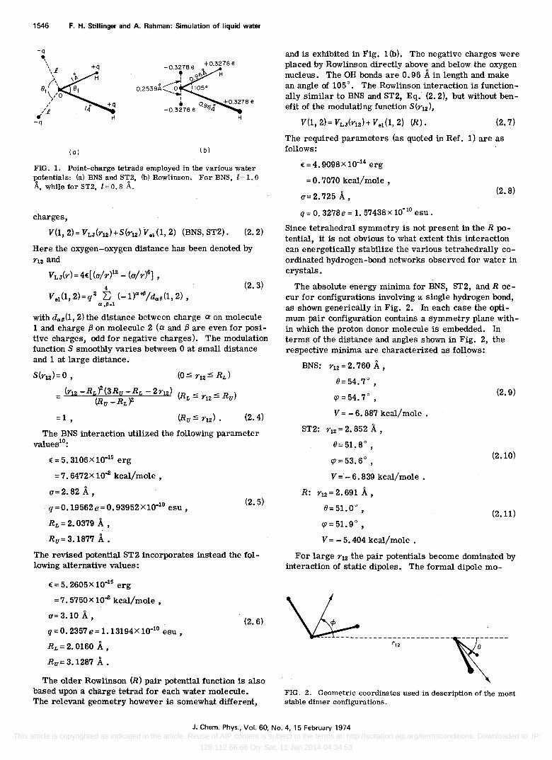
The revised pair potential (to be encoded ST2) is based on a rigid four-point-charge model for each water molecule, as was the earlier Ben-Naim and Stillinger (BNS) function. The geometry involved appears in Fig. 1 (a). The positive charges +q are identified as partially shielded protons, and have been located precisely 1 A from the oxygen nucleus, O. The distance 1 from 0 to each of the negative charges - q was also 1 A in the BNS formulation, but for the ST2 revision 1 has been reduced to 0.8 A. Pairs of vectors connecting 0 to the point charges are all disposed at the precise tetrahedral angle 6t ,

6t = 2 cos-1 (3-1 / 2)

==109°28' • (2.1)

Both the BNS and ST2 functions consist of a LennardJones central potential acting between the oxygens, plus a modulated Coulomb term for the 16 pairs of point

The Journal of Chemical Physics, Vol. 60, No.4, 15 February 1974 Copyright © 1974 American Institute of Physics 1545 This article is copyrighted as indicated in the article. Reuse of AIP content is subject to the terms at: http://scitation.aip.org/termsconditions. Downloaded to IP:

128.112.66.66 On: Sat, 11 Jan 2014 04:34:53

1546 F. H. Stillinger and A. Rahman: Simulation of liquid water

-q ~,

\\1

8tCo , ,

/.£

" -q

+q

H H

(a) ( b)

FIG. 1. Point-charge tetrads employed in the various water potentials: (a) BNS and ST2, (b) Rowlinson. For BNS, 1 = 1. 0 A, while for ST2, 1 = O. 8 A.

charges,

V(l, 2) = V LJ(r12)+S(r12) Vel (1, 2) (BNS, ST2) . (2.2)

Here the oxygen-oxygen distance has been denoted by r12 and

VLJ(r)=4E[(o/r)12 - (a/d] , 4 (2.3)

V e1 (l,2)=q2 6 (-l)a+8/daB (l, 2) , a ,B=l

with daB(l, 2)the distance between charge a on molecule 1 and charge f3 on molecule 2 (a and f3 are even for positive charges, odd for negative charges). The modulation function S smoothly varies between 0 at small distance and 1 at large distance.

= 1 , (2.4)

The BNS interaction utilized the following parameter values10:

E = 5. 3106x 10.15 erg

= 7. 6472x 10o:! kcal/mole ,

a= 2. 82 A , q=0.19562e=0.93952 x 10-10 esu,

RL = 2.0379 A , Ru= 3.1877 A •

(2.5)

The revised potential ST2 incorporates instead the following alternative values:

E = 5. 2605x 10-15 erg

= 7. 5750X 10o:! kcal/mole ,

a= 3.10 A , q = 0.2357 e = 1. 13194X 10.10 esu ,

R L =2.0160 A, Ru= 3.1287 A .

(2.6)

The older Rowlinson (R) pair potential function is also based upon a charge tetrad for each water molecule. The relevant geometry however is somewhat different,

and is exhibited in Fig. 1 (b). The negative charges were placed by Rowlinson directly above and below the oxygen nucleus. The OR bonds are 0.96 A in length and make an angle of 105 0

• The Rowlinson interaction is functionally similar to BNS and ST2, Eq. (2.2), but without benefit of the modulating function S(r12),

(2.7)

The required parameters (as quoted in Ref. 1) are as follows:

E=4.9098x10·14 erg

= O. 7070 kcal/mole ,

a= 2. 725 A , q = O. 3278e = 1. 57438 X 10"10 esu.

(2.8)

Since tetrahedral symmetry is not present in the R potential, it is not obvious to what extent this interaction can energetically stabilize the various tetrahedrally coordinated hydrogen-bond networks observed for water in crystals.

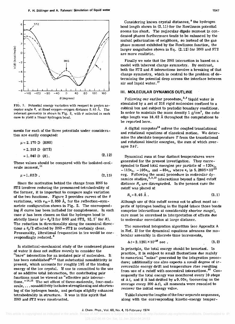
The absolute energy minima for BNS, ST2, and R occur for configurations involving a single hydrogen bond, as shown generically in Fig. 2. In each case the optimum pair configuration contains a symmetry plane within which the proton donor molecule is embedded. In terms of the distance and angles shown in Fig. 2, the respective minima are characterized as follows:

BNS: r12 = 2.760 A , 8=54.7 0

,

cp = 54.7 0 ,

V = - 6. 887 kcal/mole .

ST2: r12 = 2. 852 A , 8= 51. 8 0

,

cp=53.6°,

V = - 6. 839 kcal/mole .

R: r12 = 2. 691 A , 8= 51.0 0

,

cp = 51. 9 0 ,

V = - 5. 404 kcal/mole .

(2.9)

(2.10)

(2.11)

For large r12 the pair potentials become dominated by interaction of static dipoles. The formal dipole mo-

~2 8

FIG. 2. Geometric coordinates used in description of the most stable dimer configurations.

J. Chem. Phys., Vol. 60, No.4, 15 February 1974 This article is copyrighted as indicated in the article. Reuse of AIP content is subject to the terms at: http://scitation.aip.org/termsconditions. Downloaded to IP:

128.112.66.66 On: Sat, 11 Jan 2014 04:34:53

F. H. Stillinger and A. Rahman: Simulation of liquid water

6

4

2

Q) '. "0 E 0 "-0

~ u ~ -2 ~

§ .) >

~ '. -4

-6

-160 -120 -80 -40 o 40 80 120 160

8(degrees)

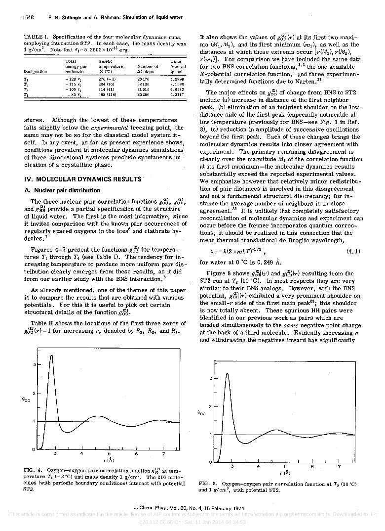
FIG. 3. Potential energy variation with respect to proton acceptor angle 6, at fixed oxygen-oxygen distance 2.85 A. The relevant geometry is shown in Fig. 2, with ~ selected in each case to yield a linear hydrogen bond.

ments for each of the three potentials under consideration are easily computed:

jJ. = 2. 170 D (BNS)

= 2. 353 D (ST2)

= 1. 840 D (R). (2.12)

These values should be compared with the isolated-molecule moment, 11

jJ.=1.83D. (2.13)

Since the motivation behind the change from BNS to ST2 involves reducing the pronounced tetrahedrality of the former, it is important to compare angle variation of the two functions. Figure 3 provides curves of the 8 variations, with r12 = 2. 850 A, for the reflection-symmetric configuration shown in Fig. 2. The corresponding R curve has been included for completeness. In each case cp has been chosen so that the hydrogen bond is strictly linear (cp = 8/2 for BNS and ST2, 52.5° for R). The reduction in directionality along the canonical directions ± 8/2 effected by BNS - ST2 is certainly clear. Presumably, librational frequencies in ice would be correspondingly reduced. 8

In statistical-mechanical study of the condensed phases of water it does not suffice merely to consider the "bare" interaction for an isolated pair of molecules. It has been established12,13 that substantial nonadditivity is present, which accounts for roughly 15% of the binding energy of the ice crystal. If one is committed to the use of an additive total interaction, the contributing pair functions must be viewed as "effective pair interactions." 14,15 The net effect of three-molecule, four-molecule, ., . nonadditivity includes strengthening and shortening of the hydrogen bonds, and perhaps slightly enhanced tetrahedl'ality in structure. It was in this spirit that BNS and ST2 were constructed.

1547

ConSidering known crystal distances, 6 the hydrogen bond length shown in (2.11) for the Rowlinson potential seems too short. The mqlecular dipole moment in condensed phases furthermore tends to be enhanced by the mutual polarization of neighbors, so instead of the gas phase moment exhibited by the Rowlinson function, the larger magnitudes shown in Eq. (2.12) for BNS and ST2 are more realistic.

Finally we note that the BNS interaction is based on a model with inherent charge symmetry. By contrast, both the ST2 and R interactions involve a breaking of that charge symmetry, which is central to the problem of determining the potential drop across the interface between air and liquid water. 17

III. MOLECULAR DYNAMICS OUTLINE

Following our earlier procedure, 2,3 liquid water is simulated by a :set of 216 rigid molecules confined to a cubical box and subject to periodic boundary conditions. In order to maintain the mass density 1 g/cm3, the cube edge length was 18.62 A throughout the computations to be reported here.

A digital computer18 solves the coupled translational and rotational equations of classical motion. We determine the absolute temperature T from the translational and rotational kinetic energies, the sum of which averages 3kT.

Dynamical runs at four distinct temperatures were generated for the pres~nt investigation. They corresponded to fixed total energies per particle of - 120(11 -115(11 -105(11 and -85(10 where (1 is 5. 2605 X 10-15

erg. Following the usual procedure in molecular dynamics studies,2,3,19 interactions beyond a fixed cutoff distance Rc are disregarded. In the present case the cutoff was placed at

Rc= 8.46 A . (3.1)

Although use of this cutoff seems not to affect most aspects of hydrogen bonding in the liquid (since those bonds comprise interactions at considerably shorter range), care must be exercised in interpretation of effects due to molecular correlation at large distance.

The numerical integration algorithm (see Appendix A in Ref. 2) for the dynamical equations advances the molecular assembly in discrete time increments,

At=2.1261x10-16 sec. (3.2)

In prinCiple, the total energy should be invariant. In practice, it is subject to small fluctuations due mainly to numerical "noise" generated by the integration procedure; additionally one also expects a small degree of irreversible energy drift and temperature rise resulting from use of a cutoff with noncentral interactions. 2o Consequently the total energy was monitored every 10 steps of A t, and if it had drifted by ± 0.05(1 (occurring on the average every 200 A t), all momenta were rescaled to recover the initial energy value.

Table I shows the lengths of the four separate sequences, along with the corresponding kinetic-energy temper-

J. Chern. Phys., Vol. 60, No.4, 15 February 1974 This article is copyrighted as indicated in the article. Reuse of AIP content is subject to the terms at: http://scitation.aip.org/termsconditions. Downloaded to IP:

128.112.66.66 On: Sat, 11 Jan 2014 04:34:53


TABLE I. Specification of the four molecular dynamics runs, employing interaction ST? In each case, the mass density was 1 g/cm3

• Note that Ej=5.2605x10-j5 erg.

Total Kinetic Time energy per temperature, Number of interval

Designation molecule OK (OC) At steps (psec)

T, -120 " 270 (-3) 23470 4.9899 T2 -115 " 284 (10) 38130 8.1068 T3 -105 " 314 (41) 21910 4.6583 T4 -85 " 392 (118) 20280 4.3117

atures. Although the lowest of these temperatures falls slightly below the experimental freezing point, the same may not be so for the classical model system itself. In any event, as far as present experience shows, conditions prevalent in molecular dynamics simulations of three-dimensional systems preclude spontaneous nucleation of a crystalline phase.

IV. MOLECULAR DYNAMICS RESULTS

A. Nuclear pair distribution

The three nuclear pair correlation functions g~J, g/}J, and g~J provide a partial specification of the structure of liquid water. The first is the most informative, since it invites comparison with the known pair occurrences of regularly spaced oxygens in the ices6 and clathrate hydrates. 7

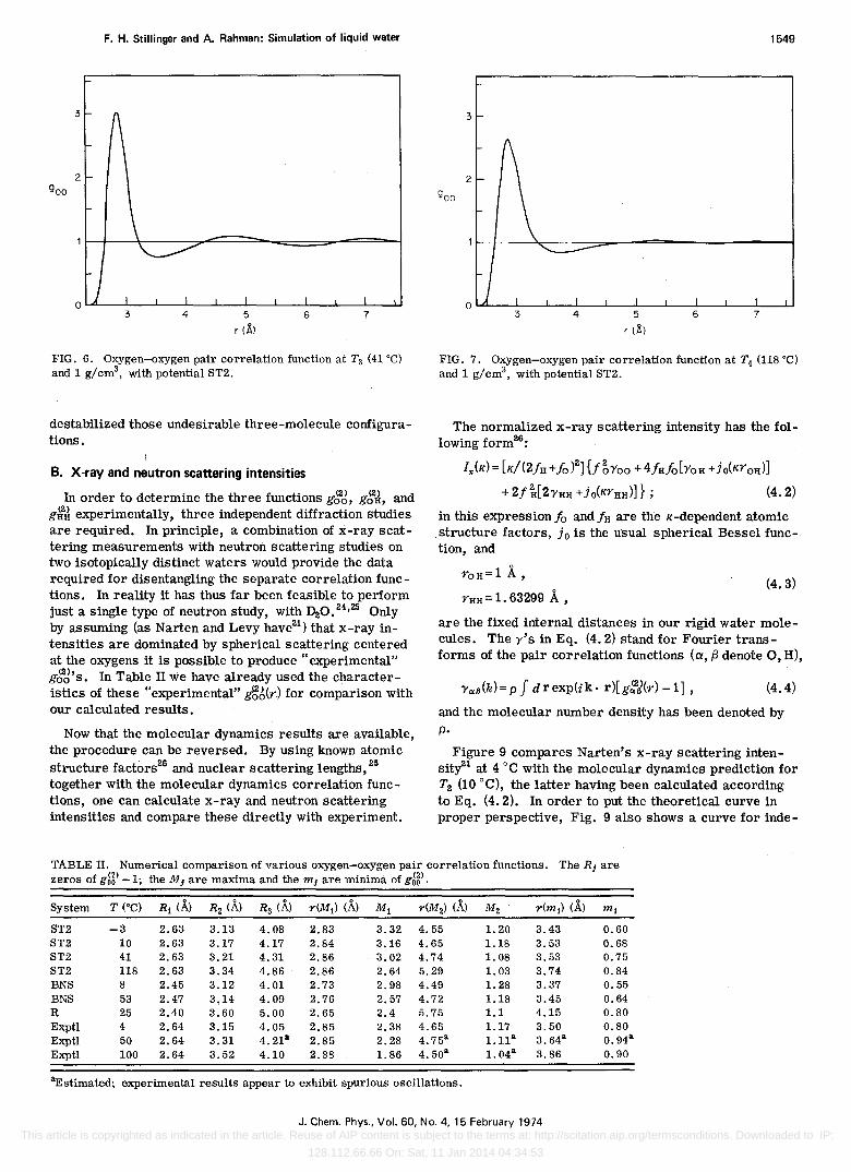
Figures 4-7 present the functions g~J for temperatures T1 through T4 (see Table I). The tendency for increaSing temperature to produce more uniform pair distribution clearly emerges from these results, as it did from our earlier study with the BNS interaction. 3

As already mentioned, one of the themes of this paper is to compare the results that are obtained with various potentials. For this it is useful to pick out certain structural details of the function g~J.

Table II shows the locations of the first three zeros of gi,2J(r) -1 for increasing r, denoted by Rh R2 , and R 3 •

3

2

FIG. 4. Oxygen-oxygen pair correlation functiong~5) at temperature T j (- 3°C) a"D.d mass density 1 g/cm3• The 216 molecules (with periodic boundary conditions) interact with potential ST2.

It also shows the values of g~ci(r) at its first two maxima (Mh M 2), and its first minimum (m1), as well as the distances at which these extrema occur [r(M1 ), r(M2 ),

r(m1)]. For comparison we have included the same data for two BNS correlation functions, 2,3 the one available R-potential correlation function,l and three experimentally determined functions due to Narten. 21

The major effects on gi,2J of change from BNS to ST2 include (a) increase in distance of the first neighbor peak, (b) elimination of an incipient shoulder on the lowdistance side of the first peak (especially noticeable at low temperature previously for BNS-see Fig. 1 in. Ref. 3), (c) reduction in amplitude of successive oscillations beyond the first peak. Each of these changes brings the molecular dynamics results into closer agreement with experiment. The primary remaining disagreement is clearly over the magnitude M1 of the correlation function at its first maximum-the molecular dynamics results substantially exceed the reported experimental values. We emphasize however that relatively minor redistribution of pair distances is involved in this disagreement and not a fundamental structural discrepancy; for instance the average number of neighbors is in close agreement. 22 It is unlikely that completely satisfactory reconciliation of molecular dynamics and experiment can occur before the former incorporates quantum corrections; it should be realized in this connection that the mean thermal translational de Broglie wavelength,

AT = h(2 1f mkT)-1/2 , (4.1)

for water at O°C is 0.249 A. Figure 8 shows g~J(r) and g~J(r) resulting from the

ST2 run at Tz (10°C). In most respects they are very similar to their BNS analogs. However, with the BNS potential, g~J(r) exhibited a very prominent shoulder on the small-r side of the first main peakZ3

; this shoulder is now totally absent. These spurious HH pairs were identified in our previous work as pairs which are bonded simultaneously to the same negative point charge at the back of a third molecule. Evidently increasing (J

and withdrawing the negatives inward has significantly

3

2

FIG. 5. Oxygen-oxygen pair correlation function at T2 (10°C) and 1 g/cm3

, with potential ST2.


128.112.66.66 On: Sat, 11 Jan 2014 04:34:53


3

2

3 4 5 6 7

r (Al

FIG. 6. Oxygen-oxygen pair correlation function at Ts (41°C) and 1 g/cms, with potential ST2.

destabilized those undesirable three-molecule configurations.

B. X-ray and neutron scattering intensities

In order to determine the three functions g~6, g~J, and g~J experimentally, three independent diffraction studies are required. In principle, a combination of x-ray scattering measurements with neutron scattering studies on two isotopically distinct waters would provide the data required for disentangling the separate correlation functions. In reality it has thus far been feasible to perform just a single type of neutron study, with DaO. 24,25 Only by assuming (as Narten and Levy have21

) that x-ray intensities are dominated by spherical scattering centered at the oxygens it is possible to produce" experimental" g&'s. In Table II we have already used the characteristics of these "experimental" iJ6(r) for comparison with our calculated results.

Now that the molecular dynamics results are available, the procedure can be reversed. By using known atomic structure factors26 and nuclear scattering lengths, 25

together with the molecular dynamics correlation functions, one can calculate x-ray and neutron scattering intensities and compare these directly with experiment.

1549

FIG. 7. Oxygen-oxygen pair correlation function at T4 (118°C) and 1 g/cms, with potential ST2.

The normalized x-ray scattering intensity has the following form26

:

I,,(K) = [K/(2/H + fo )2] {j ~yoo + 4/Hfo [YOH + io(Kr OH)]

+ 2fM2YHH +jo(KrHH )]} ; (4.2)

in this expression fo and /H are the K-dependent atomic ,structure factors, jo is the usual spherical Bessel function, and

rOH= 1 A, (4.3)

rHH = 1. 63299 A , are the fixed internal distances in our rigid water molecules. The Y'S in Eq. (4.2) stand for Fourier transforms of the pair correlation functions (a, f3 denote 0, H),

(4.4)

and the molecular number density has been denoted by p.

Figure 9 compares Narten's x-ray scattering intensitt1 at 4°C with the molecular dynamics prediction for T2 (10 DC), the latter having been calculated according to Eq. (4_ 2). In order to put the theoretical curve in proper perspective, Fig. 9 also shows a curve for inde-

TABLE II. Numerical comparison of various oxygen-oxygen pair correlation functions. The RJ are zeros of g~a) -1; the M J are maxima and the mJ are minima of g~a) .

System T (OC) Rl Cg,) R2 (A) Rs (A) r(M1) (A) Ml r(M2) (A) M2 r(ml) (A) ml

ST2 -3 2.63 3.13 4.08 2.83 3.32 4.55 1. 20 3.43 0.60 ST2 10 2.63 3.17 4.17 2.84 3.16 4.65 1.18 3.53 0.68 ST2 41 2.63 3.21 4.31 2.86 3.02 4.74 1. 08 3.53 0.75 ST2 118 2.63 3.34 4.86 2.86 2.64 5.29 1. 03 3.74 0.84 BNS 8 2.45 3.12 4.01 2.73 2.98 4.49 1.28 3.37 0.55 BNS 53 2.47 3.14 4.09 2.76 2.57 4.72 1.18 3.45 0.64 R 25 2.40 3.60 5.00 2.65 2.4 5.75 1.1 4.15 0.80 Exptl 4 2.64 3.15 4.05 2.85 2.38 4.65 1.17 3.50 0.80 Exptl 50 2.64 3.31 4.21a 2.85 2.28 4.75a l.11a 3.64a 0.94a Exptl 100 2.64 3.52 4.10 2.88 1.86 4.50a 1. 04a 3.86 0.90

aEstimated; experimental results appear to exhibit spurious oscillations.


128.112.66.66 On: Sat, 11 Jan 2014 04:34:53


1.8,----------------------,

1.6

1.4

1.2

1.0 1-----++'-~H-;....:."__--=:.....,.._~_:::-~:=,=...",-----4

0.8

0.6

0.4

0.2

~

/ /

O~ _ _L~_~_~ __ ~_~ __ ~_~ _ __J

o 2 3 5 6 7 8

FIG. 8. Oxygen-hydrogen and hydrogen-hydrogen pair correlation functions at T2 (1o°C) and 1 g/cm3• The interaction employed is ST2. Only the intermolecular pairs are shown.

pendent molecule scattering [just the terms containing jo in Eq. (4.2)]. The Significant magnitude of this independent-molecule scattering, especially at small K,

makes it important eventually to assess the quantitative validity of the spherical scattering approximation-we consider this to be an important open problem.

The agreement in Fig. 9 between theory and experiment is moderately good, and includes a tendency of the former to exhibit the characteristic double peak around 2. 5 .A.-1 that seems to be unique to water. We anticipate that agreement will be improved by allowing the theoretical calculation to incorporate both intramolecular vibrations, as well as quantum corrections.

The x-ray scattering intenSity calculated earlier for the BNS potential2 was too strongly damped at large K.

Evidently the passage to ST2 has improved that situation. Similarly, the double peak around 2.5 .A.-1 was, for BNS, less impressive than the one shown in Fig. 9 for ST2.

The neutron scattering intensity In may be written in a form analogous to that for 1,,:

In(K) = (2aD+1lo)-2{~i'oo +4aDllo[YoD+jo(KroD)]

(4.5)

The K-independent coherent scattering lengths for the deuteron and the 160 nucleus have been denoted by aD and 00, respectively. Of course the molecular dynamics Simulation, in its structural aspects, makes no distinction between D and H, i. e., i'DD =i'HH, etc.

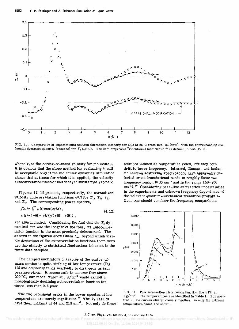
Figure 10 presents the theoretical and experimental neutron scattering curves for comparison. The theoretical curve has again been computed from the T2 (10°C) dynamical run. The experimental determination is Narten's at 25°C. Again the principal features of the two curves agree, though systematic discrepancies are clearly present.

Neutrons are a far more sensitive probe of hydrogen isotope arrangement than are x rays. Furthermore these light nuclei experience substantial vibrational amplitudes which are not explicitly represented in the molecular dynamics simulation. We have therefore tested the importance of hydrogen vibrations, using rms deviations suggested by Narten,25 on the function In(K). Mter inserting the appropriate "phenomenological" Gaussian factors into Eq. (4.5), the discrepancies shown in Fig. 10 around 4 and 8 .A.-1 are substantially reduced (by a factor of 2 or better). The "theoretical" result however still possesses it smaller main peak at 2 .A.-1 than experiment.

If both experimental 1" and In curves are to be accepted as accurate indicators of nuclear order in water, then one might tentatively conclude that oxygen nuclei in the simulation are somewhat too ordered spatially, and hydrogen nuclei not ordered enough. But conSidering the various soUrces of imprecision in both experiment and Simulation, it seems premature at present to draw firm conclusions.

C. Pair interaction distribution

In our earlier study of temperature effects in water, S

it proved useful to evaluate p(V), the distribution function for pair interaction energy. In an N -molecule system it may be defined as follows:

p(V) = c (o[V - V(1, 2)]) N

= [2c/N(N -1)] L; < O[V - V(i,j)]) , (4.6) 1<1=1

where the constant c depends on the specific normalization of convenience. Naturally p(V) vanishes when parameter V is less than the absolute minimum of the effective pair potential V(i,j). Furthermore for a large molecular system p (V) becomes very large for V ~ 0 on account of the great population of widely separated, weakly interacting pairs.

Although p(V) was originally introduced to describe systems with additive interactions, we stress in passing that a natural generalization exists to accommodate potential energy nonadditivity. In the most general case, the total potential will have the form

N N

L; L; V (n) (i 1 ••• in) , (4.7) n:2 It< ... <l n=l

with explicit occurrence of pair, triplet, quadruplet, •• " N -tuplet potentials. For n> 2, one can consider that each v(n) is symmetrically distributed among the nCn -1)/2 molecule pairs involved, so that the quantity V(i,j) appearing in definition (4.6) of p(V) above should be replaced by

N N L; L; [2/nCn-1)]v(n)(i,j,i s '" in) • (4.8) n:2 Is< ... <lnal

(#/ .J)

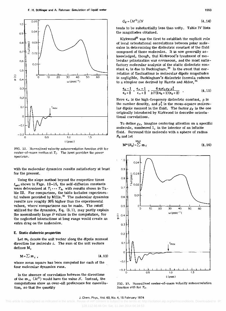
The interaction distributions extracted from the four ST2 dynamical runs are shown in Fig. 11. As in the case of the BNS potential, we again have a nearly invariant point at a negative V. From Fig. 11 we see that


128.112.66.66 On: Sat, 11 Jan 2014 04:34:53

1.0

-1.0


. ...

1551

FIG. 9. Comparison of x-ray scattering intensity measured for water at 4°C (Ref. 21), with the corresponding intensity derived from the T2 (10°C) molecular dynamics. The latter uses independent atomic scattering factors. Experimental results are denoted by discrete points. Curves A and B are theoretical results, with A just the intramolecular scattering, while B is the complete scattering prediction. '

the value of V for ST2 is - 4. 0 kcal/mole (for BNS it was - 3.7 kcal/mole), with some indication that this point at which

ap(V)jaT=O (4.9)

drifts toward slightly larger VasT increases to T4 (118°C).

We conclude from the behavior of p(V) as a function of temperature that, in our model, water exhibits a basic hydrogen-bond rupture mechanism with a dynamic equi-· librium between pairs interacting with energy less than - 4. 0 kcal/mo1e and those with an energy just above that value. We estimate the mean excitation energy across the fixed point to be 2.9 kcal/mo1e. 27

Figure 11 shows p(V) declining monotonically for positive V. This contrasts with the prior BNS case for which a "spurious" maximun'l occurs around 2.5 kcal/mo1e. 28

This maximum arose from those configurations (two molecules with protons bound Simultaneously by the same

negative charge of a third) which gave g:fJ an undesired small-distance shoulder, and which, as we have previously observed, are eliminated by ST2.

D. Self-diffusion process

In an infinite system at equilibrium, the self -diffusion constant D may be obtained from the long-time limit of the mean-square displacement of a selected molecule j,

D=lim{ ([~RJ(t)]2)/6t}. (4.10) t _00

In what follows ~R J(t) refers specifically to the displacement of the center of mass for molecule j over time interval t, though any other fixed poSition in the molecule would serve as well (such as the oxygen or a hydrogen nucleus position). Because molecular dynamiCS Simulations are limited in both space and time, it is necessary to infer D from the slope of «~ R J)2) vs t. One has the identity

(d/dt)([~RJ(m2)=2J;/dt'(VJ(0).vJ(t'», (4.11)


128.112.66.66 On: Sat, 11 Jan 2014 04:34:53


o.4r---------------------------------------------------------------------,

0.3 I-

0.2 - x

x. 0.1 I- x

:.:: 0

t: H

xXxxx x •••••••••• :: x x ••••• • ••• ~ •••••

"x XX" X X X X X

X X

-0.1 -

-0.2 I- ~ x x (>.¥.x'"'1« ...x x x...... ~ ......... .

--------------------x~~ •• ~ •• ~~--------~~~~rv."x~x~x~x'~~t~~""~O x x ¥.~.~ ~ ••••• ~.; ...... .. ~. "~ ~.

.~.¥.~. VIBRATIONAL MODIFICATION -0.3 I-x

-0.4 I I I I I I I I I I I I 0 2 3 4 5 6 7 8 9 10 11 12

K (A-1)

FIG. 10. Comparison of experimental neutron diffraction intensity for D20 at 25°C from Ref. 25 (dots), with the corresponding molecular dynamics quantity (crosses) for T2 (10°C). The semiempirical "vibrational modification" is defined in Sec. IV. B.

where vJ is the center-of -mass velocity for molecule j. It is obvious that the slope method for evaluating D will be acceptable only if the molecular dynamics simulation shows that at times for which it is applied, the velocity autocorrelation function has decayed substantially to zero.

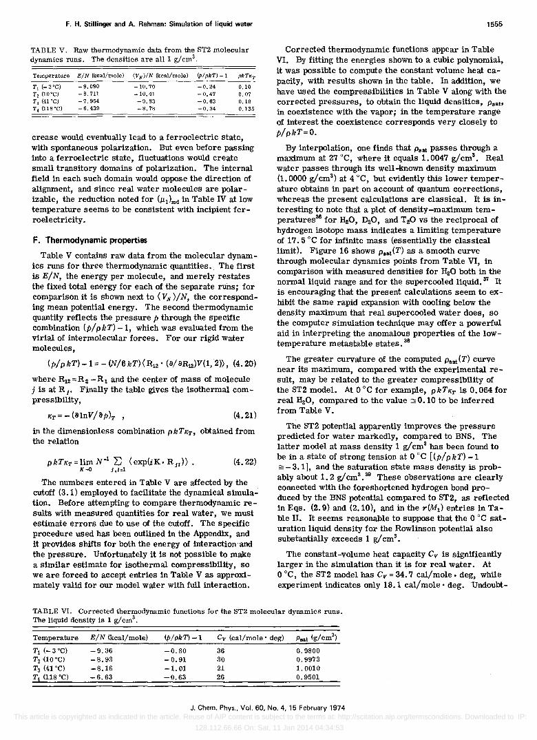
Figures 12-15 present, respectively, the normalized velocity autocorrelation functions cp (t) for Ta, T2 , T3 ,

and T4 • The corresponding power spectra,

j(w) = fa'" cp(t) cos (wt)dt ,

cp(t)=(v(O). v(t)/(v(O). v(O) , (4.12)

are also included. Considering the fact that the Ta,dynamical run was the longest of the four, its autocorrelation function is the most precisely determined. The arrows in the figures show times tmax beyond which visible deviations of the autocorrelation functions from zero are due strictly to statistical fluctuations inherent in the finite data samples.

The damped OSCillatory character of the center-ofmass motion is quite striking at low temperature (Fig. 12) and obviously tends markedly to disappear as temperature rises. It seems safe to assume that above 200°C, our model water at 1 g/cm3 would exhibit a monotonically declining autocorrelation function for times less than 0.5 psec.

The two prominent peaks in the power spectra at low temperature are surely significant. 29 The T2 results have their maxima at 44 and 215 em-I. Not only do these

features weaken as temperature rises, but they both drift to lower frequency. Infrared, Raman, and inelastic neutron scattering spectroscopy have apparently detected broad translational bands in roughly these two frequency region ('" 60 cm-l and in the range 150-200 cm-I).30 ConSidering base-line subtraction uncertainties in the experiments and unknown frequency dependence of the relevant quantum-mechanical transition probabilities, one should consider the frequency comparisons

0.007

0.006

0.005

0.004

p(v)

0.003

0.002

0.001

V(kcal/mole)

FIG. 11. Pair interaction distribution function (for ST2) at 1 g/cm3

• The temperatures are identified in Table 1. For positive V, the curves cluster closely together, so only the extreme temperature cases are shown.


128.112.66.66 On: Sat, 11 Jan 2014 04:34:53

1.0

0.9

0.8

0.7

0.6

0.5

::.--e- 0.4

0.3

0.2

0.1

0

-0.1

-0.2 0


U Q) U> 0.

] -

0.05

0.04

0.03

0.02

0.01

O~--~--~----~---L----~--~--~ o 10 20 30 40 50 60

w(psec-')

1.0

t(psec)

FIG. 12. Normalized velocity autocorrelation function cp(t) for center-of-mass motion at T1 • The inset provides the power spectrum.

with the molecular dynamics results satisfactory at least for the present.

Using the slope method beyond the respective times tmax shown in Figs. 12-15, the self-diffusion constants were determined at Tl ••• Th with results shown in Table ill. For comparison, the table includes experimental values provided by Mills. 31 The molecular dynamics results are roughly 30% higher than the experimental values, where' comparisons can be made. The cutoff utilized for the dynamiCS, Eq. (3.1), may partly explain the anomalously large D values in the computation, for the neglected interactions at long range would create an extra drag on the molecules.

E. Static dielectric properties

Let m t denote the unit vector along the dipole moment direction for molecule i. The sum of the unit vectors defines M,

(4.13)

whose mean square has been computed for each of the four molecular dynamics runs.

In the absence of correlation between the directions of the m" (M2) would have the value N. Instead, the computations show an over-all preference for cancellation, so that the quantity

1553

(4.14)

tends to be substantially less than unity. Table IV lists the magnitudes obtained.

Kirkwood32 was the first to establish the explicit role of local orientational correlations between polar molecules in determining the dielectric constant of the fluid composed of those molecules. It is now generally acknowledged, though, that Kirkwood's treatment of molecular polarization was erroneous, and the most satisfactory molecular analysis of the static dielectric constant Eo is due to Buckingham. 33 In the event that correlation of fluctuations in molecular dipole magnitudes is negligible, Buckingham's dielectric formula reduces to a simpler one derived by Harris and Alder, 34

Eo - 1 == E", - 1 + 4 1rpEOgK p.i Eo + 2 Eo> + 2 kT(2 Eo + l)(Eo+ 2)

(4.15)

Here Eo> is the high-frequency dielectric constant, pis the number density, and p.~ is the mean-square molecular dipole moment in the fluid. The factor gK is the one originally introduced by Kirkwood to describe orientational correlations.

To define gK, imagine centering attention on a specific molecule, numbered 1, in the interior of an infinite fluid. Surround this molecule with a sphere of radius Ro and let

(4.16)

1.0 0.04

0.9

U 0.03 Q)

0.8 U>

..9-~ _ 0.02

0.7

0.6 0.01

0.5 o~--~--~----~--~----~--~--~

_ 0.4 G-

0.3

0.2

0.1

o 10 20 30 40

w(psec- 1 )

50 60

°rt~~----~~~~-------------------4

-0.1

0.5 1.0

t(psec)

1.5

FIG. 13. Normalized center-of-mass velocity autocorrelation function cp(t) for T 2•


128.112.66.66 On: Sat, 11 Jan 2014 04:34:53


0.05 1.0

0.9 0.04

U Q) Vl

0.8 .9- 0.03 ]

0.7 0.02

0.6 0.01

0.5

:;:; 0.4

."..

oOL----1~0----2~0--~3~0----4LO----5LO----6LO~--~

w (psec- 1)

0.3

0.2

0.1

~ tmax

O~+-~--~~--------------------------~

-0.1

_0.2L-L-~~-L-L-L~~L-L-L-~~-L-L-L~~L-~

o 0.5 1.0 1.5

Upsec)

FIG. 14. Normalized center-of-mass velocity autocorrelation function cp(t) for T3, with its corresponding power spectrum.

be the sum of unit vectors for molecules within the sphere. Then

gK=lim m 1 • M*(Ro) • (4.17) RO~""

Deviations of gK above unity measure the extent to which the neighbors of molecule 1 locally align their dipoles along m 1. The double limit involved in definition of gK (infinite system size, followed by Ro- 00) is crucial and prevents equality of gK and GK• For the molecular dynamics procedure utilized here, it has been argued2 that

(4.18)

No direct means is available in the molecular dynamics method, as presently constituted, to evaluate dielectric constants. Still we can insert measured dielectric constants into Eq. (4.18) to estimate the Kirkwood fac-

TABLE III. Comparison of self-diffusion constants D from the present molecular dynamiCS Simulation, and from experiment (Ref. 31). The units for Dare 10-5

cm2/sec.

Temperature D (mol. dyn) D (exptI)

T1 (-3 ec) 1.3 1. 00 T2 (10 ec) 1.9 1. 55 Ts (41°C) 4.3 3.32 T4 (118°C) 8.4

TABLE IV. Dielectric properties for the water simulation. The static (EO) and optical-frequency (E",,) dielectric constants are experimental values for 1 g/ cm3

•

Temperature GK EO E"" gK (!il)md (!iI)OJlSager

T1 (_3°C) 0.18 88.9 1. 78 3.66 1.84 D 2.30 D T2 (10°C) 0.15 83.8 1. 78 2.88 2.06 D 2.30 D T3 (41 ec) 0.16 72.8 1. 77 2.68 2.09 D 2.29 D T4 (118 ec) 0.21 51. 4 1. 75 2.52 2.02 D 2.27 D

tor gK. Table IV lists the rel~vant (0 values from experiment, and the resulting gK'S.

Having once obtained gK, it is possible to employ the Harris-AIder-Buckingham formula, Eq. (4.15), to calculate the liquid-phase mean dipole moment ill' For that purpose it is also necessary to use the measured ("" listed in Table IV (we have used the square of the refractive index at the frequency of the sodium D line). The results are listed as (ill)md in Table IV and should be compared to the moment suggested by Onsager, 35

(4.19)

which can be obtained from the vapor moment ilv = 1. 83 D (values are included in the table).

The rapid increase of gK as temperature declines through T1 implies a marked tendency for local alignment of the water molecules. Continuation of that in-

1.0

0.9

0.8

0.7

0.6

0.5

:;:; 0.4

."..

0.3

0.2

0.1

0

-0.1

0.04

U Q)

~0.03

~

0.02

0.01

O~ __ ~ __ ~ ____ L-__ -L __ ~~ __ ~ __ ~ o 10 20 30 40 50

w (psec- 1 )

t(psec)

60

FIG. 15. Normalized center-of-mass velocity autocorrelation function cp(t) for T4 and its associated power spectrum (inset).

J. Chern. Phys .• Vol. 60. No.4, 15 February 1974 This article is copyrighted as indicated in the article. Reuse of AIP content is subject to the terms at: http://scitation.aip.org/termsconditions. Downloaded to IP:

128.112.66.66 On: Sat, 11 Jan 2014 04:34:53


TABLE V. Raw thermodynamic data from the ST2 molecular dynamics runs. The densities are alII g/cm8

Temperature E/N (kcal/mole) (VN)/N (kcal/mole) (P/pkT) -1 pkTK r T, (_3°C) -9.090 -10.70 -0.24 0.10 T, (10°C) - 8. 711 -10.41 -0.47 0.07 T3 (41°C) -7.954 -9.83 -0.63 0.10 T, (118°C) -6.439 -8.78 -0.34 0.135

crease would eventually lead to a ferroelectric state, with spontaneous polarization. But even before passing into a ferroelectric state, fluctuations would create small transitory domains of polarization. The internal field in each such domain would oppose the direction of alignment, and since real water molecules are polarizable, the reduction noted for (P.l)md in Table IV at low temperature seems to be consistent with incipient ferroelectricity.

F. Thermodynamic properties

Table V contains raw data from the molecular dynamics runs for three thermodynamic quantities., The first is E/N, the energy per molecule, and merely restates the fixed total energy for each of the separate runs; for comparison it is shown next to (VN )/N, the corresponding mean potential energy. The second thermodynamic quantity reflects the pressure p through the specific combination (p/ pkT) -1, which was evaluated from the virial of intermolecular forces. For our rigid water molecules,

(p/ P kT) -1 == - (N/6 kT) (R12 • (8/ 8R12)V(1,2), (4.20)

where R12 ::: R 2 - R 1 and the center of mass of mOlecule j is at R J. Finally the table gives the isothermal compressibility,

/(T=-(8lnV/ap)T , (4.21)

in the dimensionless combination pkTKT' obtained from the relation

(4.22)

The numbers entered in Table V are affected by the cutoff (3.1) employed to facilitate the dynamical simulation. Before attempting to compare thermodynamic results with measured quantities for real water, we must estimate errors due to use of the cutoff. The specific procedure used has been outlined in the Appendix, and it provides shifts for both the energy of interaction and the pressure. Unfortunately it is not possible to make a similar estimate for isothermal compressibility, so we are forced to accept entries in Table V as approximately valid for our model water with full interaction.

1555

Corrected thermodynamic functions appear in Table VI. By fitting the energies shown to a cubic polynomial, it was possible to compute the constant volume heat capacity, with results shown in the table. In addition, we have used the compressibilities in Table V along with the corrected pressures, to obtain the liquid densities, PS&t,

in coexistence with the vapor; in the temperature range of interest the coexistence corresponds very closely to p/pkT=O.

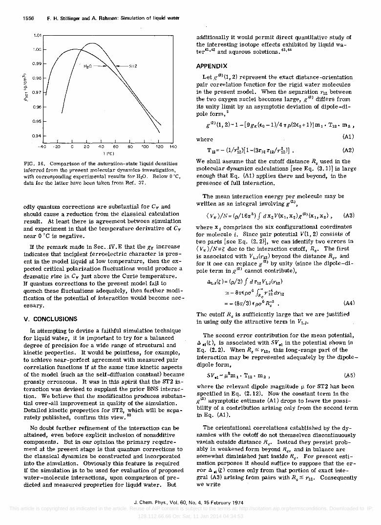
By interpolation, one finds that Put passes through a maximum at 27°C, where it equals 1.0047 g/cm3

• Real water passes through its well-known denSity maximum (1. 0000 g/cm3

) at 4°C, but evidently this lower temperature obtains in part on account of quantum corrections, whereas the present calculations are classical. It is interesting to note that a plot of density-maximum temperatures36 for H20, D20, and T20 vs the reciprocal of hydrogen isotope mass indicates a limiting temperature of 17.5 °c for infinite mass (essentially the classical limit). Figure 16 shows psat(T) as a smooth curve through molecular dynamics points from Table VI, in comparison with measured densities for H20 both in the normal liquid range and for the supercooled liquid.:rI It is encouraging that the present calculations seem to exhibit the same rapid expansion with cooling below the density maximum that real supercooled water does, so the computer Simulation technique may offer a powerful aid in interpreting the anomalous properties of the lowtemperature metastable states. 38

The greater curvature of the computed psat(T) curve near its maximum, compared with the experimental result' may be related to the greater compressibility of the ST2 model. At 0 °c for example, pkT/(T is 0.064 for real H20, compared to the value ~ 0.10 to be inferred from Table V.

The ST2 potential apparently improves the pressure predicted for water markedly, compared to BNS. The latter model at mass density 1 g/ cm3 has been found to be in a state of strong tension at 0 °c [(p/ P kT) -1 ~ - 3. 1], and the saturation state mass density is probably about 1. 2 g/cm3

• 39 These observations are clearly connected with the foreshortened hydrogen bond produced by the BNS potential compared to ST2, as reflected in Eqs. (2.9) and (2.10), and in the r(Ml) entries in Table II. It seems reasonable to suppose that the 0 °c saturation liquid density for the Rowlinson potential also substantially exceeds 1 g/cm3

•

The constant-volume heat capacity Cv is significantly larger in the simulation than it is for real water. At o °c, the ST2 model has Cv = 34.7 cal/mole. deg, while experiment indicates only 18.1 cal/mole' deg. Undoubt-

TABLE VI. Corrected thermodynamic functions for the ST2 molecular dynamics runs. The liquid density is 1 g/cms .

Temperature E/N (kcal/mole) (P/pkT) -1 Cv (cal/mole· deg) Psat (g/cms)

Tl (_3°C) -9.36 -0.80 36 0.9800 T2 (10°C) -8.93 -0.91 30 0.9973 Ts (41°C) -8.16 -1.01 21 1. 0010 T4 (118°C) -6.63 -0.63 26 0.9501


128.112.66.66 On: Sat, 11 Jan 2014 04:34:53

1556

'" E " "-

'"


1.01 r----------------------,

0.94

-40 -20 o 20 40 60 80 100 120 140

T (Oel

FIG. 16. Comparison of the saturation-state liquid densities inferred from the present molecular dynamics investigation, with corresponding experimental results for H20. Below 0 cC, data for the latter have been taken from Ref. 37.

edly quantum corrections are substantial for Cv and should cause a reduction from the classical calculation result. At least there is agreement between simulation and experiment in that the temperature derivative of C y

near 0 DC is negative.

If the remark made in Sec .. IV.E that the gK increase indicates that incipient ferroelectric character is present in the model liquid at low temperature, then the expected critical polarization fluctuations would produce a dramatic rise in C y just above the Curie temperature. If quantum corrections to the present model fail to quench these fluctuations adequately, then further modification of the potential of interaction would become necessary.

V. CONCLUSIONS

In attempting to devise a faithful simulation technique for liquid water, it is important to try for a balanced degree of precision for a wide range of structural and kinetic properties. It would be pointless, for example, to achieve near-perfect agreement with measured pair correlation functions if at the same time kinetic aspects of the model (such as the self-diffusion constant) became grossly erroneous. It was in this spirit that the ST2 interaction was devised to supplant the prior BNS interaction. We believe that the modification produces substantial over-all improvement in quality of the simulation. Detailed kinetic properties for ST2, which will be separately published, confirm this view. 40

No doubt further refinement of the interaction can be attained, even before explicit inclusion of nonadditive components. But in our opinion the primary requirement at the present stage is that quantum corrections to the classical dynamics be constructed and incorporated into the simulation. Obviously this feature is required if the simulation is to be used for evaluation of proposed water-molecule interactions, upon comparison of predicted and measured properties for liquid water. But

additionally it would permit direct quantitative study of the interesting isotope effects exhibited by liquid water41 ,42 and aqueous solutions. 43,44

APPENDIX

Let g(2) (1,2) represent the exact distance-orientation pair correlation function for the rigid water molecules in the present model. When the separation r12 between the two oxygen nuclei becomes large, g(2) differs from its unity limit by an asymptotic deviation of dipole-dipole form, 5

g(2) (1,2)-1 - [9gK (Eo -1)/41T p(2Eo + 1)] mI' T12 • m2 ,

where (AI)

(A2)

We shall assume that the cutoff distance Re used in the molecular dynamiCS calculations [see Eq. (3.1)] is large enough that Eq. (AI) applies there and beyond, in the presence of full interaction.

The mean interaction energy per molecule may be written as an integral involving g(2),

(VN >/N = (p/1611 2) J d X2 V(Xb x 2 ) g(2) (Xl, X2) , (A3)

where x I comprises the six configurational coordinates for molecule i. Since pair potential V(l, 2) consists of two parts [see Eq. (2.2)], we can identify two errors in (VN)/N==i;, due to the interaction cutoff, Re. The first is associated with VLJ(r12) beyond the distance Re, and for it one can replace g(2) by unity (since the dipole-dipole term in g(2) cannot contribute),

.:lLJ(i;,)= (p/2) J dr12VLJ(r12)

6 r~ -4 == - 811Epu JR r 12 dr12 e

= _ (811/3) Epu G R~3 . (A4)

The cutoff Re is suffiCiently large that we are justified in using only the attractive term in VLJ•

The second error contribution for the mean potential, .:leI (i;,), is associated with SVOI in the potential shown in Eq. (2.2). When Re:5 r12, this long-range part of the interaction may be represented adequately by the dipoledipole form,

(A5)

where the relevant dipole magnitude f1 for ST2 has been specified in Eq. (2.12). Now the constant term in the g(2) asymptotic estimate (AI) drops to leave the possibility of a contribution ariSing only from the second term in Eq. (AI).

The orientational correlations established by the dynamics with the cutoff do not themselves discontinuously vanish outside distance Re. Instead they persist probably in weakened form beyond R e , and in balance are somewhat diminished just inside Re. For present estimation purposes it should suffice to suppose that the error .:leI (i;,) comes only from that portion of exact integral (A3) ariSing from pairs with Re:5 r12. Consequently we write


128.112.66.66 On: Sat, 11 Jan 2014 04:34:53


Ael(b)= ~ f dX2(p.2ml· Tl2 0 m2)

Rc ~r12

X (_ 9gK~E:o -1)) m l' T12 • m2) 41TP 2E:o + 1

The multiple integrals may be carried out to give

Ael (b)= - p.2 gK(E:o -1)/(2E:o + l)R~ •

Equations (A4) and (A7) together give the correction A(b) for the interaction energy.

(A6)

(A7)

The virial equation of state shown in Eq. (4.20) may be written in terms of gtZ) as follows:

(p/ pkT) - 1 == ~

= - (p/481T 2kT) J d X 2[r12' (a/ar12 ) V(l, 2)]g(Z).

The cutoff error for~, A(~), likewise has two parts~A8) ALJ(~) and Ael (~), analogous to those that arise for the potential energy~ They can be evaluated in virtually the same fashion:

(A9)

(Al0)

The two "LJ" corrections can immediately be evaluated from the potential parameters in Eq. (2.6). The "el" corrections, however, require p. from Eq. (2.12) and the semiempirical quantity gK and measured E:o listed in Table IV.

"Part of the work carried out at the Argonne National Laboratory was supported by the U. S. Atomic Energy Commission.

IJ. A. Barker and R. O. Watts, Chern. Phys. Lett. 3, 144 (1969).

2A. Rahman and F. H. Stillinger, J. Chern. Phys. 55, 3336 (1971).

3F . H. Stillinger and A. Rahman, J. Chern. Phys. 57, 1281 (1972).

4S. A. Rice and P. Gray, The Statistical Mechanics of Simple Liquids (Wiley-Interscience, New York, 1965).

5A. Ben-Nairn and F. H. Stillinger, "Aspects of the StatisticalMechanical Theory of Water, " in Structure and Transport Processes in Water and Aqueous Solutions, edited by R. A. Horne (Wiley-Interscience, New York, 1972).

6D. Eisenberg and W. Kauzmann, The Structure and Properties of Water (OxfordU. P., New York, 1969), Chap. 3.

7L . Pauling, The Nature of the Chemical Bond (Cornell U. P., Ithaca, NY, 1960), p. 469.

80 . Weres and S. A. Rice, J. Am. Chern. Soc. 94, 8983 (1972).

9J . S. Rowlinson, Trans. Faraday Soc. 47, 120 (1951). lOIn Refs. 2 and 3 it was found desirable to renormalize the

strength of the orginally proposed BNS potential (Ref. 5) with a factor 1. 06. The quantities € arid q2 scale upwards accordingly. In this paper ~'BNS" will henceforth refer exclusively to the renormalized function.

l1Referelilce 6, p. 12.

1557

12D. Hankins, J. W. Moskowitz, and F. H. Stillinger, J. Chern. Phys. 53, 4544 (1970); s~e also Erratum, J. Chern. Phys. 59, 995 (1973).

13B . R. Lentz and H. A. Scheraga, J. Chern. Phys. 58, 5296 (1973).

14F . H. Stillinger, J. Phys. Chern. 74, 3677 (1970). 15F . H. Stillinger, J. Chern. Phys. 57, 1780 (1972). 16W• H. Flygare and R. C. Benson, Mol. Phys. 20, 225 (1971). 17F. H. Stillinger and A. Ben-Nairn, J. Chern. Phys. 47, 4431

(1967). 18We have employed the IBM 360/195 at the Argonne National

Laboratory for the work reported in this paper. 19A. Rahman, Phys. Rev. 136, A405 (1964). 20In test runs with At chosen as one-quarter of the value shown

in Eq. (3.2), the numerical "noise" was virtually eliminated, and we were unable to observe any clear secular temperature rise. Evidently the cutoff irreversibility is a minor consideration over the length of the usual dynamical runs.

21A. H. Narten and H. A. Levy, J. Chern. Phys. 55, 2263 (1971). We are grateful to Dr. Narten for supplying us with tables for g~5) (r) prepared from structure functions given in this paper.

22The 4 °C pair distribution reported in Ref. 21 implies an average of 5.3 neighbors within 3.53 A, while the ST2 result at 10°C yields 5.5 neighbors within the same distance Uts r(m1), see Table Ill.

23Reference 3, Fig. 5. 24D. 1. Page and J. G. Powles, Mol. Phys. 21, 901 (1971). 25A. H. Narten, J. Chern. Phys. 56, 5681 (1972). 26A. H. Narten, ONRL Rept. No. ONRL-4578, July 1970. 27For this estimate, ap/aT was constructed from the T2 and T3

curves in Fig. 11. The region for which this derivative is negative (V < - 4 kcal/mole) has roughly the same area as the region of positive derivative just above - 4 kcal/mole. The difference in mean v.alues of V for the two adjacent regions is the quoted excitation energy .

28Reference 3, Fig. 11. 29Similar behavior was previously observed for the BNS inter-

action. 30Reference 6, Table 4.10. 31R . Mills, J. Phys. Chern. 77, 685 (1973). 32J • G. Kirkwood, J. Chern. Phys. 7, 911 (1939). 33A. D. Buckingham, Proc. Roy. Soc. A 238, 235 (1956). 34F . E. Harris and B. J. Alder, J. Chern. Phys. 21, 1031

(1953). 35L . Onsager, J. Am. Chern. Soc. 58, 1486 (1936). 36Reference 6, Table 4.3, p. 187. 37B. V. Zheleznyi, Russ. J. Phys. Chern. 43, 1311 (1969). 38C. A. Angell, J. Shuppert, and J. C. Tuckedto be published). 39A. Rahman, in "Molecular Dynamics and Monte Carlo Cal-

culations on Water," report of a C.E.C.A.M. Workshop held in Orsay, France, 19 June-12 August 1972; see speCifically. pp. 41 and 57.

4°F. H. Stillinger and A. Rahman, in Proceedings of the 24th International Meeting, "Molecular Motion in Liquids," of the Societe de Chimie Physique, PariS, 3-6 July 1973 (to be published).

41W. M. Jones, J. Chern. Phys. 48, 207 (1968). 42F • J. Millero and F. K. Lepple, J. Chern. Phys. 54, 946

(1971). 43E . E. Schrier, R. J. Loewinger, and A. H. Diamond, J.

Phys. Chern. 70, 586 (1966). 44B . E. Conway and L. H. Laliberte, J. Phys. Chern. 72,

4317 (1968).


128.112.66.66 On: Sat, 11 Jan 2014 04:34:53

Documents

Improved simulation of liquid water by molecular dynamics*fhs/paper66/paper66.pdf · Improved simulation of liquid water by molecular ... Carlo"l and the "molecular dynamics,,2.3