4.3 Improper Integrals

In the previous section, we defined Riemann integral for functions defined on closed and

bounded interval [a, b]. In this section our aim is to extend the concept of integration to

the the following cases:

1. The function f(x) defined on unbounded interval [a,∞) and f ∈ R[a, b] for allb > a.

2. The function is not defined at some points on the interval [a, b].

We first consider

Improper integral of first kind: Suppose f is a bounded function defined on [a,∞)

and f ∈ R[a, b] for all b > a.

Definition 4.3.1. The improper integral of f on [a,∞) is defined as

∫ ∞

a

f(x)dx := limb→∞

∫ b

a

f(x)dx.

If the limit exists and is finite, we say that the improper integral converges. If the limit

goes to infinity or does not exist, then we say that the improper integral diverges.

Examples:

1. (i)∫∞1

1x2dx = limb→∞

∫ b

11x2dx = limb→∞ 1− 1

b= 1.

2. (ii)∫∞0

dx1+x2 = limb→∞

∫ b

0dx

1+x2 = limb→∞ arctanxb0 =

π2.

Theorem 4.3.2. Comparison test: Suppose 0 ≤ f(x) ≤ φ(x) for all x ≥ a, then

1.∫∞a

f(x)dx converges if∫∞a

φ(x)dx converges.

2.∫∞a

φ(x)dx diverges if∫∞a

f(x)dx diverges.

Proof. Define F (x) =∫ x

af(t)dt and G(x) =

∫ x

ag(t)dt. Then by properties of Riemann

integral, 0 ≤ F (x) ≤ G(x) and we are given that limx→∞

G(x) exists. So G(x) is bounded.

F is monotonically increasing and bounded above. Therefore, limx→∞

F (x) exists.

Examples:

1.∫∞1

dxx2(1+ex)

. Note that 1x2(1+ex)

< 1x2 and

∫∞1

dxx2 converges.

15

2.∫∞1

x3

x+1dx. Note that x3

x+1> x2

2on [1,∞) and

∫∞1

x2dx diverges.

Definition 4.3.3. Let f ∈ R[a, b] for all b > a. Then we say∫∞a

f(x)dx converges

absolutely if∫∞a|f(x)|dx converges.

In the following we show that absolutely convergence implies convergence of improper

integral.

Theorem 4.3.4. If the integral∫∞a|f(x)|dx converges, then the integral

∫∞a

f(x)dx con-

verges.

Proof. Note that 0 ≤ f(x) + |f(x)| ≤ 2|f(x)|. So the improper integral∫∞a

f(x) +

|f(x)|dx converges by comparison theorem above. Also∫∞a|f(x)| converges. Therefore,∫∞

af(x)dx =

∫∞a

f(x) + |f(x)|dx− ∫∞a|f(x)|dx also converges. ///

The converse of the above theorem is not true. For example take the integral∫∞π

sinxxdx.

This integral does not converge absolutely. Indeed,

∫ ∞

π

| sin x|x

dx =∞∑n=1

∫ (n+1)π

nπ

| sin x|x

dx

≥∞∑n=1

1

nπ

∫ (n+1)π

nπ

| sin x|

=∞∑n=0

1

nπ

∫ π

0

sin x =2

π

∞∑n=1

1

n.

On the other hand, by integration by parts,

limb→∞

∫ b

1

sin x

xdx = lim

b→∞

∫ b

1

1

xd(1− cos x)

= limb→∞

((1− cos b

b+

∫ b

1

1− cosx

x2dx

)

It is not difficult to show that the limits on the right exist.

Examples:

1.∫∞1

sinxx3 dx. Easy to see that | sinx

x3 | ≤ | 1x3 | and∫∞1

dxx3 converges.

2.∫∞0

e−x2 sinxlog(1+x)

. Here first note that limx→0e−x2 sinxlog(1+x)

= 1. Therefore the integral is proper

16

at x = 0. For x > 10(say):

|f(x)| ≤ e−x2

log(1 + x)< e−x

2 ≤ e−x

Hence the integral∫∞10

e−x2 sinxlog(1+x)

converges by comparison theorem.

Theorem 4.3.5. Limit comparison test: Let f(x), g(x) are defined and positive for

all x ≥ a and limx→∞

f(x)

g(x)= L.

1. If L ∈ (0,∞), then the improper integrals∫∞a

f(x)dx and∫∞a

g(x)dx are either both

convergent or both divergent. i.e.,∫∞a

f(x)dx converges ⇐⇒ ∫∞a

g(x) converges.

2. If L = 0, then∫∞a

f(x)dx converges if∫∞a

g(x)dx converges. i.e,∫∞a

g(x)dx con-

verges =⇒ ∫∞a

f(x)dx converges.

3. If L =∞, then∫∞a

f(x)dx diverges if∫∞a

g(x)dx diverges. i.e.,∫∞a

g(x)dx diverges

=⇒ ∫∞a

f(x)dx diverges.

Proof. From the definition of limits, for any ε > 0, there exists M > 0 such that

x ≥M =⇒ L− ε <f(x)

g(x)< L+ ε.

Thus for x ≥M , we have (L− ε)g(x) < f(x) < (L+ ε)g(x).

Now in case (1), since L > 0, we can find ε > 0 such that L− ε > 0. Using the property 3,

it is enough to prove the convergence/divergence for x large, say x ≥M . In this interval,

we have the comparison (L− ε)g(x) < f(x) < (L + ε)g(x). Now integrating this, we get

the result.

In case (2), we have f(x) < (L+ ε)g(x). Again, integrate on both sides.

In case (3) by the definition, for every M > 0, there exists, R such that f(x) > Mg(x)

for all x > R. Now the result follows similar to (1) and (2).

Examples:

1.∫∞1

dx√x+1

. Take f(x) = 1√x+1

and g(x) = 1√x. Then limx→∞

f(x)g(x)

= 1 and∫∞1

g(x)dx

diverges. So by above theorem,∫∞1

f(x)dx diverges.

2.∫∞1

dx1+x2 . Take f(x) = 1

1+x2 and g(x) = 1x2 . Then limx→∞

f(x)g(x)

= 1 and∫∞1

g(x)dx

converges. So by above theorem,∫∞1

f(x)dx converges.

17

3.∫∞0

xcoshx

dx. Let f(x) = xcoshx

= 2xex

e2x+1∼ xe−x. So choose g(x) = xe−x. Then

limx→∞f(x)g(x)

= 2 and∫∞0

g(x) converges.

Improper integrals of second kind

Definition 4.3.6. Let f(x) be defined on [a, c) and f ∈ R[a, c − ε] for all ε > 0. Then

we define ∫ c

a

f(x)dx = limε→0

∫ c−ε

a

f(x)dx.

Then∫ b

af(x)dx is said to converge if the limit exists and is finite. Otherwise, we say

improper integral∫ b

af(x)dx diverges.

Example:

∫ 1

0

dx√x= lim

ε→0

∫ 1

ε

dx√x= lim

ε→02(1−√ε) = 2.

Suppose a1, a2, ....an are finitely many discontinuities of f(x) in [a, b]. Then

∫ b

a

f(x)dx =

∫ a1

a

f(x)dx+

∫ a2

a1

f(x)dx+

∫ a3

a2

f(x)dx+ ....+

∫ b

an

f(x)dx

If all the improper integrals on the right hand side converge, then we say the improper

integral of f over [a, b] converges. Otherwise, we say it diverges.

The following comparison and Limit comparison tests can be proved following similar

arguments:

Theorem 4.3.7. (Comparison Theorem:) Suppose 0 ≤ φ(x) ≤ f(x) for all x ∈ [a, c) andare discontinuous at c.

1. If∫ c

af(x)dx converges then

∫ c

aφ(x)dx converges.

2. If∫ c

aφ(x)dx diverges then

∫ c

af(x)dx diverges.

Theorem 4.3.8. (Limit comparison theorem:) Suppose 0 < f(x), g(x) be continuous in

[a, c) and limx→cf(x)g(x)

= L. Then

1. If L ∈ (0,∞). Then∫ c

af(x)dx and

∫ c

ag(x)dx both converge or diverge together.

2. If L = 0 and∫ c

ag(x)dx converges then

∫ c

af(x)dx converges.

3. If L =∞ and∫ c

ag(x)dx diverges then

∫ c

af(x)dx diverges.

18

Proof. From the definition of limit, for each ε > 0, there exists δ > 0 such that

x ∈ (c− δ, c) =⇒ (L− ε)g(x) < f(x) < (L+ ε)g(x)

Rest of the proof follows in the similar lines theorems on first kind, by choosing ε < L.

Transforming improper integrals:

Sometimes improper integrals may be transformed into proper integrals. for example

consider the improper integral I =

∫ 3

1

dx√x√3− x

. Taking the transformation y =1

3− x,

we get I =

∫ ∞

1/2

dy

y√3y − 1

. This is an improper integral of first kind. Instead, if we choose

the transformation 3− x = u2 then I =

∫ √2

0

2udu√u√3− u2

, which is a proper integral.

Remark 4.6. It is important to note that the ”symmetric” limit could be convergent but

the limit may not exist. For example,

∫ 1

−1

dx

x3=

∫ 0

−1

dx

x3+

∫ 1

0

dx

x3

= limε1→0

∫ −ε1

−1

dx

x3+ lim

ε2→0

∫ 1

ε2

dx

x3

=1

2lim

ε1,ε2→0(1

ε21− 1

ε22), (4.7)

where ε1, ε2 → 0 as n→∞. It is easy to see that if one takes ε1 = ε2, then the limit exits

and is equal to 0. But if one takes ε1 =1

(n+1)2, ε2 =

1n2 , then the above limit in (4.7) does

not exist. So through different sequences, we are getting different limits. By now, by our

familiarity with existence of limits, we say integral diverges.

Gamma and Beta functions:

Consider the Gamma function defined as improper integral for p > 0,

Γ(p) =

∫ ∞

0

xp−1e−xdx

This integral is improper of first kind in the neighbourhood of 0 as xp−1 goes to infinity as

x→∞ (when p < 1). Since the domain of integration is (0,∞), the integral is improper

19

of first kind. To prove the convergence, we divide the integral into

Γ(p) =

∫ 1

0

xp−1e−xdx+∫ ∞

1

xp−1e−xdx

=I1 + I2

To see the convergence of I1 we take f(x) = xp−1e−x and g(x) = xp−1, then limx→0

f(x)

g(x)= 1

and

∫ 1

0

xp−1dx converges. To see the convergence of I2, take f(x) = xp−1e−x and

g(x) = 1x2 . Then lim

x→∞f(x)

g(x)= lim

x→∞x2+p−1e−x = 0 and

∫∞1

1x2dx converges. Hence by

(2) of limit comparison theorem, the integral converges.

Next we consider the Beta function defined as improper integral for p > 0, q > 0,

β(p, q) =

∫ 1

0

xp−1(1− x)q−1dx

If p > 1 and q > 1, then the integral is definite integral. When p < 1 and/or q < 1, this

integral is improper of second kind at 0 and/or 1. To prove the convergence, we divide as

before

∫ 1

0

xp−1(1− x)q−1dx =∫ 1/2

0

xp−1(1− x)q−1dx+∫ 1

1/2

xp−1(1− x)q−1dx

= I1 + I2.

To see the convergence of I1, take f(x) = xp−1(1 − x)q−1 and g(x) = xp−1. Then

limx→0

f(x)

g(x)= lim

x→0(1 − x)q−1 = 1 and

∫ 1/2

0

xp−1dx converges. Similarly, for convergence

of I2, we take f(x) = xp−1(1− x)q−1 and g(x) = (1− x)q−1.

Some identities of beta and gamma functions:

1. Γ(1) =∫∞0

e−xdx = 1.

2. Γ(α + 1) = αΓ(α).

Integration by parts formula implies,

Γ(α + 1) =

∫ ∞

0

xαe−x = −(xαe−x)|∞0 +

∫ ∞

0

xα−1e−xdx = αΓ(α).

20

Therefore, Γ(m+ 1) = m! ∀m ∈ IN .

3. Γ(12) =

√π.

(Γ(1

2)

)2

=4

∫ ∞

0

∫ ∞

0

e−u2

e−v2

dudv, take u = r cos θ, v = r sin θ,

=4

∫ ∞

0

∫ π/2

0

e−r2

rdrdθ = π

4. β(m,n) = β(n,m). Substituting t = 1− x in the definition of β(m,n), we get

β(m,n) =

∫ 1

0

tn−1(1− t)m−1dt = β(n,m)

5. β(m,n) = 2

∫ π/2

0

sin2m−1 θ cos2n−1 θdθ

Taking x = cos2 θ in β(m,n), we get

β(m,n) =

∫ π

0

cos2m−2 θ sin2n−2 θ cos θ sin θdθ = 2

∫ π/2

0

cos2m−1 θ sin2n−1 θdθ.

6. β(m,n) = Γ(m)Γ(n)Γ(m+n)

.

Problem: Evaluate (i)

∫ ∞

0

x2/3e−√xdx (ii)

∫ 1

0

x32 (1−√x)

12dx

For (i), take t =√x, then the given integral becomes

∫ ∞

0

t4/3e−t2tdt = 2

∫ ∞

0

e−tt7/3dt = 2Γ(10

3) =

56

27Γ(1/3).

For (ii), again take t =√x, then the integral becomes

2

∫ 1

0

t3(1− t)1/2tdt = 2

∫t4(1− t)1/2dt = 2β(5, 3/2) = 2

Γ(5)Γ(3/2)

Γ(13/2)=

512

3465

Cauchy Principal Value:

Consider the improper integral I =∫∞0sin xdx. It is easy to see from the definition that

I = lima→∞(1− cos a) which does not exist.Similarily,∫ 0−∞ sin xdx does not exist. But

limc→∞

∫ c

−csin xdx

21

exists and is equal to 0. Though the improper integral does not exist, this symmetric

limit exists. This is called Cauchy Principal value of improper integral

Definition 4.3.9. The Cauchy Principal value of improper integral of first kind is defined

as

CPV

∫ ∞

−∞f(x)dx = lim

R→∞

∫ R

−Rf(x)dx

For the improper integral of second kind, with c ∈ (a, b) as point of discontinuity of f(x)

as

CPV

∫ b

a

f(x)dx = limδ→0

∫ c−δ

a

f(x)dx+

∫ b

c+δ

f(x)dx

Examples:

First kind:∫∞−∞ x2n+1dx for all n = 1, 2, 3, .... In this case it is easy to check that

lima→∞

∫ a

−ax2n+1 = 0. But the the improper integrals

∫∞0

x2n+1 and∫ 0−∞ x2n+1 does not

converge.

Second kind:∫ 1−1 x

−(2n+1)dx, for n = 1, 2, 3, .... Simply evaluate

∫ −ε

−1x−(2n+1) +

∫ 1

ε

x−(2n+1)

to see that the the limit is 0.

Integrals dependent on a Parameter

Cosider an integral

I(α) =

∫ b

a

f(x, α)dx

where the integrand is depend on the parameter α. At times we can differentiate under

the integral sign to evaluate the integral. It is sometimes not possible and leads to wrong

assertions. For example, we know that I =∫∞0

sinxx

= π2. It is easy to notice with change

of variable formula, taking tx = y, that I = I(t) =∫∞0

sin(tx)x

= π2. Now differentiating

this, taking derivative inside integral, we get I ′(t) =∫∞0cos(tx)dx = 0, which doesn’t

make sense.

Here we have a theorem, which explains under which conditions we can do the differenti-

ation under integral sign.

Theorem 4.3.10. Suppose,

22

1. Suppose f, ddαf(x, α) are continuous functions for x ∈ [a, b] and α in an interval of

containing α0.

2. |f(x, α)| ≤ a(x), | ddαf(x, α)| ≤ b(x) such that a, b are integrable on [a, b].

Then I is differentiable, and

I ′(α) =∫ b

a

d

dαf(x, α)dx.

Proof. .

d

dαI(α) = lim

Δα→0

I(α +Δα)− I(α)

Δα

= lim1

Δα

[∫ b

a

(f(x, α +Δα)− f(x, α))dx

]

Now by Taylor’s theorem, f(x, α+Δα)− f(x, α) = Δα ddαf(x, α+ θΔα). Since d

dαf(x, α)

is continuous, we have ddαf(x, α + θΔα) = d

dαf(x, α) + ε, where 0 < θ < 1 and ε → 0 as

Δα→ 0. Thus

d

dαI(α) = lim

Δα→0

∫ b

a

d

dαf(x, α) + ε =

∫ b

a

d

dαf(x, α)dx

///

In fact the following holds.

Newton-Leibnitz Formula:

Let h(x) =

∫ b(x)

a(x)

f(x, t)dt. Then h′(x) =∫ b(x)

a(x)

df

dx(x, t)dt+f(x, b(x))b′(x)−f(x, a(x))a′(x)

Examples:

1. Evaluate I(α) =

∫ ∞

0

e−xsinαx

xdx.

By the above formula, I ′(α) =∫∞0

e−x cosαxdx = 11+α2 . Therefore, I(α) = arctanα+

C. Also I(0) =∫∞0

e−x sin 0x = 0. Hence C = 0.

2. Test the convergence and evaluate the integral

∫ ∞

0

e12(t2−x2) cos(tx)dx.

|I| ≤∫ ∞

0

|e−x2

cos(tx)|dx ≤ C

∫ ∞

0

e−x2

dx =1

2Γ(1

2).

23

Hence the integral converges. By Newton Leibnitz formula,

I ′a(t) =∫ a

0

e12(t2−x2)(t cos tx− x sin tx)dx

=

∫ a

0

∂

∂xe

12(t2−x2) sin txdx

= e12(t2−a2) sin at

Therefore, I ′(t) = lima→∞ I ′a(t) = 0. Now note that I(0) =∫∞0

e−x2/2dx = Γ(1/2).

Hence I(t) =√

π2.

4.4 Approximation of definite integrals

Suppose we are given a function f : [a, b]→ IR that is integrable on [a, b] and has its Taylor

series in an interval containing [a, b]. Then we can approximate the definite integral using

the Taylor series. Let f(x) =∑∞

k=0 antn for |t| < R. Then we know from the term-

by-term integration theorem,

∫ t

0

f(x)dx =∞∑k=0

∫ t

0

anxndx =

∞∑k=0

antn+1

n+ 1|t| < R

Example: Find the approximate value of the definite integral∫ 10x2 sin(x2)dx with error

less than 10−4.

We note that if the nth term has k zeros in the first k decimals, then the approximation

is with error 10k−1.

∫ 1

0

x2 sin(x2)dx =

∫ 1

0

∞∑n=0

(−1)n x4n+4

(2n+ 1)!

=∞∑n=0

(−1)nx4n+5(4n+ 5)(2n+ 1)!

10

=∞∑n=0

(−1)n(4n+ 5)(2n+ 1)!

Hence ∫ 1

0

x2 sin(x2) =1

5− 1

54+

1

13× 5!− 1

17× 7!

Since the 4th term has 4 zeros in the first 4 decimal places. So the approximation has

error less than 10−4.

24

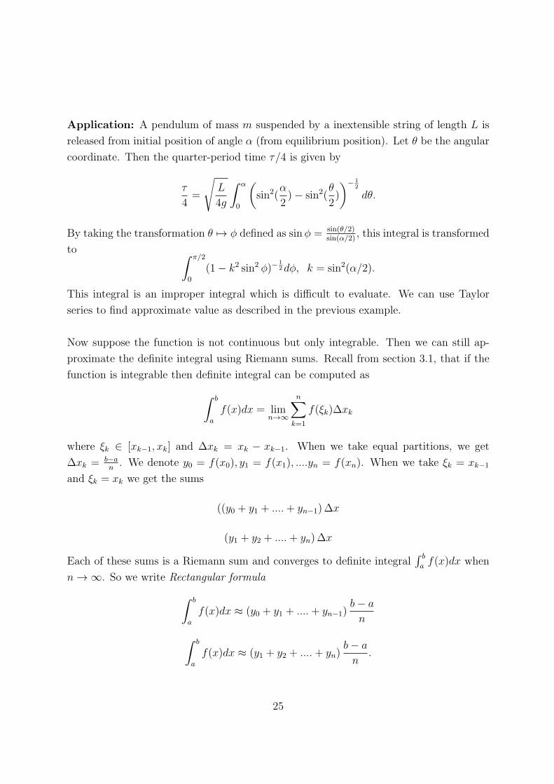
Application: A pendulum of mass m suspended by a inextensible string of length L is

released from initial position of angle α (from equilibrium position). Let θ be the angular

coordinate. Then the quarter-period time τ/4 is given by

τ

4=

√L

4g

∫ α

0

(sin2(

α

2)− sin2(

θ

2)

)− 12

dθ.

By taking the transformation θ �→ φ defined as sinφ = sin(θ/2)sin(α/2)

, this integral is transformed

to ∫ π/2

0

(1− k2 sin2 φ)−12dφ, k = sin2(α/2).

This integral is an improper integral which is difficult to evaluate. We can use Taylor

series to find approximate value as described in the previous example.

Now suppose the function is not continuous but only integrable. Then we can still ap-

proximate the definite integral using Riemann sums. Recall from section 3.1, that if the

function is integrable then definite integral can be computed as

∫ b

a

f(x)dx = limn→∞

n∑k=1

f(ξk)Δxk

where ξk ∈ [xk−1, xk] and Δxk = xk − xk−1. When we take equal partitions, we get

Δxk =b−an. We denote y0 = f(x0), y1 = f(x1), ....yn = f(xn). When we take ξk = xk−1

and ξk = xk we get the sums

((y0 + y1 + ....+ yn−1)Δx

(y1 + y2 + ....+ yn)Δx

Each of these sums is a Riemann sum and converges to definite integral∫ b

af(x)dx when

n→∞. So we write Rectangular formula

∫ b

a

f(x)dx ≈ (y0 + y1 + ....+ yn−1)b− a

n

∫ b

a

f(x)dx ≈ (y1 + y2 + ....+ yn)b− a

n.

25

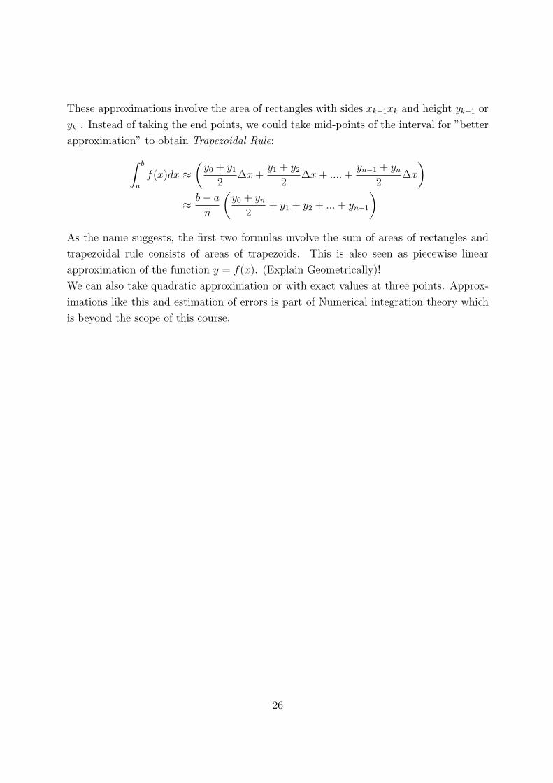
These approximations involve the area of rectangles with sides xk−1xk and height yk−1 or

yk . Instead of taking the end points, we could take mid-points of the interval for ”better

approximation” to obtain Trapezoidal Rule:

∫ b

a

f(x)dx ≈(y0 + y1

2Δx+

y1 + y22

Δx+ ....+yn−1 + yn

2Δx

)

≈ b− a

n

(y0 + yn

2+ y1 + y2 + ...+ yn−1

)

As the name suggests, the first two formulas involve the sum of areas of rectangles and

trapezoidal rule consists of areas of trapezoids. This is also seen as piecewise linear

approximation of the function y = f(x). (Explain Geometrically)!

We can also take quadratic approximation or with exact values at three points. Approx-

imations like this and estimation of errors is part of Numerical integration theory which

is beyond the scope of this course.

26

4.5 Applications to Area, Arc length, Volume and Surface area

Suppose f(x) ≥ 0 on [a, b]. Then it is clear from the definition of Definite integral that

the area under the curve y = f(x) can be approximated by Riemann sums. i.e.,

A ∼=n∑

k=1

f(ξi)(xi − xi−1)→∫ b

a

f(x)dx as n→∞.

Similarly, the area bounded by the curves y = f(x) and y = g(x) where f(x) ≥ g(x) on

[a, b] is

A =

∫ b

a

(f(x)− g(x))dx.

Example: Find the area bounded by y = x2 and y2 = x

The curves interest at x = 0, 1. The upper curve is y2 = x and lower curve is y2 = x. So

by the above formula

A =

∫ 1

0

(√x− x2)dx =

2

3− 1

3=1

3

One can also find by integrating along y: A =

∫ 1

0

(√y − y2)dy =

1

3.

Polar coordinates

A point (x, y) on the xy-plane is assigned polar coordinates (r, θ) if the point is at a dis-

tance r =√x2 + y2 from the origin on the ray at an angle θ with positive x-axis. We allow

r negative with convention: (−r, θ) = (r, θ + π). Each point on the plane has infinitely

many representations in polar form, for example (1, 0) is at a distance of 1 units from the

origin on the x-axis. So it can be represented in polar form also as (r, θ) = (1, 0). Also it is

same as (1, 2nπ), n ∈ N and (−1, π). Each point (r, θ) is same as (r, θ+2nπ) for all n ∈ N.

Example: The point (2, π/6) can also be represented by (−2, 5π6) and (−2, 7π

6)

Relation with cartesian coordinates:

We often use the following relations:

1. Given the polar coordinates (rθ), we can write the cartesian coordinates using x =

r cos θ, and y = r sin θ.

2. Given the cartesian coordinates (x, y), we can write polar coordinates using r =√x2 + y2, and θ = tan−1( y

x)

27

Circles and Straight lines:

1. The circle x2+y2 = a2 in cartesian coordinates, using (1) above, r2 cos2 θ+r2 sin2 θ =

a2 which is r = a.

2. The circle (x − a)2 + y2 = a2 =⇒ x2 + y2 − 2ax = 0, again by (1) above we get

r2 − 2ar cos θ = 0 =⇒ r = 2a cos θ.

3. The circle x2 + (y − a)2 = a2 =⇒ x2 + y2 − 2ay = 0, again by (1) above we get

r2 − 2ar sin θ = 0 =⇒ r = 2a sin θ.

4. The straight line y = mx is θ = tan−1m

5. The straight line x = a is r = a sec θ and y = b is r = b csc θ.

Symmetry in polar coordinates: The symmetry of the graph of the function in po-

lar coordinates helps one to plot/trace the graph. There are three types of symmetry

principles.

1. For (r, θ) on the graph, suppose (r,−θ) is also on the graph. Then the graph is

symmetric about x− axis.

2. For (r, θ) on the graph, suppose (r, π − θ) is also on the graph. Then the graph is

symmetric about y- axis.

3. For (r, θ) on the graph, suppose (r, π + θ) is also on the graph. Then the graph is

symmetric about the origin.

Examples:

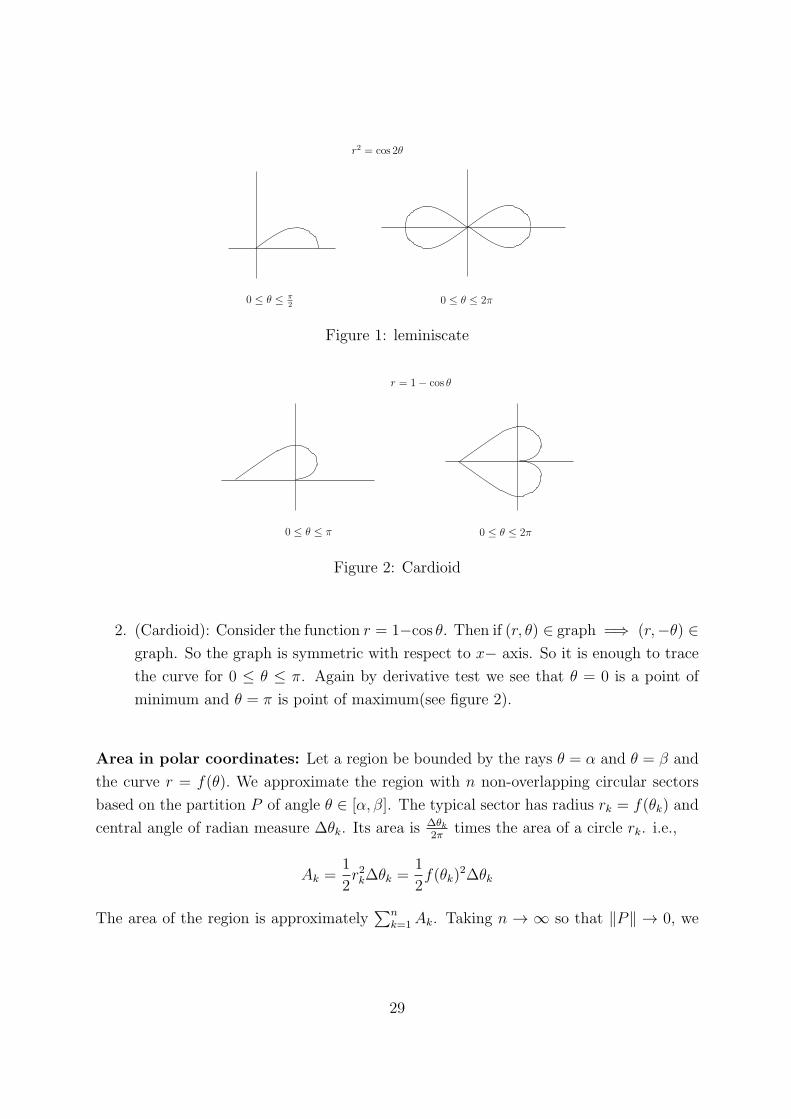
1. (leminiscate): Consider the function r2 = cos 2θ. If (r, θ) is on the graph, then

r2 = cos 2(−θ) = cos 2θ implies (r,−θ) is also on the graph. So the graph is

symmetric about x− axis.

Again, r2 = cos 2(π − θ) = cos(2π − 2θ) = cos 2θ implies (r, π + θ) is also on the

graph. Therefore, graph is symmetric about y-axis.

We can also see that (r, π + θ) is also on the graph. So the graph is also symmetric

about the origin.

Hence it is enough to trace the curve in the first quadrant. Now since r2 ≥ 0, the

domain of θ in the first quadrant is [−π4, π4]. Also one can see by the derivative test

that θ = 0 is a point of local maxima(see figure 1).

28

0 ≤ θ ≤ π2 0 ≤ θ ≤ 2π

r2 = cos 2θ

Figure 1: leminiscate

0 ≤ θ ≤ π 0 ≤ θ ≤ 2π

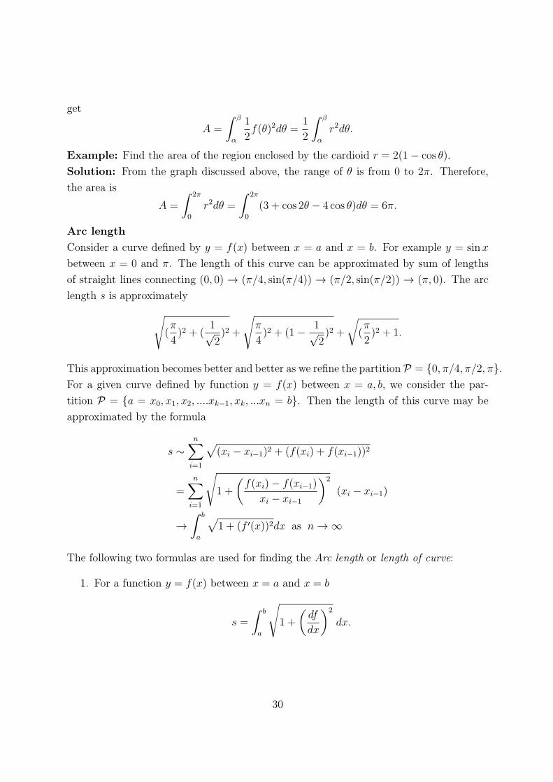
r = 1− cos θ

Figure 2: Cardioid

2. (Cardioid): Consider the function r = 1−cos θ. Then if (r, θ) ∈ graph =⇒ (r,−θ) ∈graph. So the graph is symmetric with respect to x− axis. So it is enough to trace

the curve for 0 ≤ θ ≤ π. Again by derivative test we see that θ = 0 is a point of

minimum and θ = π is point of maximum(see figure 2).

Area in polar coordinates: Let a region be bounded by the rays θ = α and θ = β and

the curve r = f(θ). We approximate the region with n non-overlapping circular sectors

based on the partition P of angle θ ∈ [α, β]. The typical sector has radius rk = f(θk) and

central angle of radian measure Δθk. Its area isΔθk2π

times the area of a circle rk. i.e.,

Ak =1

2r2kΔθk =

1

2f(θk)

2Δθk

The area of the region is approximately∑n

k=1Ak. Taking n → ∞ so that ‖P‖ → 0, we

29

get

A =

∫ β

α

1

2f(θ)2dθ =

1

2

∫ β

α

r2dθ.

Example: Find the area of the region enclosed by the cardioid r = 2(1− cos θ).

Solution: From the graph discussed above, the range of θ is from 0 to 2π. Therefore,

the area is

A =

∫ 2π

0

r2dθ =

∫ 2π

0

(3 + cos 2θ − 4 cos θ)dθ = 6π.

Arc length

Consider a curve defined by y = f(x) between x = a and x = b. For example y = sin x

between x = 0 and π. The length of this curve can be approximated by sum of lengths

of straight lines connecting (0, 0) → (π/4, sin(π/4)) → (π/2, sin(π/2)) → (π, 0). The arc

length s is approximately

√(π

4)2 + (

1√2)2 +

√π

4)2 + (1− 1√

2)2 +

√(π

2)2 + 1.

This approximation becomes better and better as we refine the partition P = {0, π/4, π/2, π}.For a given curve defined by function y = f(x) between x = a, b, we consider the par-

tition P = {a = x0, x1, x2, ....xk−1, xk, ...xn = b}. Then the length of this curve may be

approximated by the formula

s ∼n∑

i=1

√(xi − xi−1)2 + (f(xi) + f(xi−1))2

=n∑

i=1

√1 +

(f(xi)− f(xi−1)

xi − xi−1

)2

(xi − xi−1)

→∫ b

a

√1 + (f ′(x))2dx as n→∞

The following two formulas are used for finding the Arc length or length of curve:

1. For a function y = f(x) between x = a and x = b

s =

∫ b

a

√1 +

(df

dx

)2

dx.

30

2. For a function x = f(y) between y = c and y = d

s =

∫ d

c

√1 +

(df

dy

)2

dy.

Parametric form: Suppose if an arc is defined in the parametric form x = x(t), y = y(t)

between t = T1 and t = T2. Then we note from above approximation, that s may be

approximated by taking the partition P = {T1 = t0, t1, ...., tn = T2} and

s ∼n∑

i=1

√(xi − xi−1ti − ti−1

)2

+

(yi − yi−1ti − ti−1

)2

(ti − ti−1)

→∫ T2

T1

√(x′(t))2 + (y′(t))2 dt as n→∞.

Example: Find the arc length of the curve defined by x = 2 cos2 θ, y = 2 cos θ sin θ ,

0 ≤ θ ≤ π.

Solution: This curve is a circle with radius 1 at (1, 0). So the answer should be 2π.

Applying formula

s =

∫ π

0

√x′(θ)2 + y′(θ)2 dθ = 2

∫ π

0

√(2 cos θ sin θ)2 + (cos2 θ − sin2 θ)2 dθ

=2

∫ π

0

√cos4 θ + 2 cos2 θ sin2 θ + sin4 θ dθ = 2π

Example 2: Find the arc length of an arc of x23 + y

23 = 1.

Solution: Take the parametrization: x = cos3 t, y = sin3 t, 0 ≤ t ≤ π2. Then

(dx

dt

)2

+

(dy

dt

)2

= 9 cos2 t sin2 t.

Hence the arc length is

l = 3

∫ π2

0

cos t sin t dt =3

2

Problem: Find the approximate value of the length of ellipse x = a cos t, y = b sin t, 0 ≤t ≤ 2π when a = 1, e = 1/2.

solution: By the arc length formula,

l = 4a

∫ π/2

0

√1− e2 cos2 tdt

31

where e is ellipse’s eccentricity. This integral is non-elementary except when e = 0 or

1. The integrals in this form are called elliptic integrals. We can use Trapezoidal rule to

evaluate the value when a = 1 and e = 1/2. The answer with n = 10 is l = 5.870.

Suppose the curve is given in polar form r = f(θ), α ≤ θ ≤ β. Then by taking the

parametrization x = r cos θ = f(θ) cos θ and y = r sin θ = f(θ) sin θ with θ ∈ [α, β], we

getdx

dθ= f ′(θ) cos θ − f(θ) sin θ,

dy

dθ= f ′(θ) sin θ + f(θ) cos θ.

Hence the arc length is

l =

∫ β

α

√f 2(θ) + (f ′)2(θ)dθ.

Application to Work done

Suppose the force f(x) depends on position x is along a straight line from x = a to x = b.

Let n ∈ N, Δx = b−anand xi = a+ iΔx for i = 1, 2, ..., n. Then the work done in moving a

particle under the force f(x) from xk−1 to xk is approximately Wk = f(xk)Δx. The total

work done (in moving from a to b) approximately is W ∼∑ni=1 f(x

∗k)Δx, x∗k ∈ [xk−1, xk].

Taking n→∞ we get the total work done as W =∫ b

af(x)dx.

Example: Find the work required to compress a spring from its natural length of 1 foot

to a length of 0.75 foot if the force constant is k = 16 kg/foot.

Solution: Hooks law ways that the force it takes to stretch or compress a spring x length

nits from its natural length is proportional to x. i.e.,F = kx, k is constant measured in

force units per unit length.

Suppose the given springs is placed on the x− axis. It is fixed at x = 1 and movable end

at the origin. From the above formula, the force required to compress the spring from 0

to x with the formula F = 16x. To compress the spring from 0 to 0.25 ft, the force must

increase from F (0) = 0 to F (0.25) = 16× 0.25 = 4 foot-kg. Therefore, the work done by

F over this interval is

W =

∫ 0.25

0

16xdx = 0.5 ft− kg.

Volume of ”symmetrical” objects

Method of Slicing:

Consider a solid lying alongside some interval [a, b] of the x-axis. For each x let A(x) be the

area of the cross section (of the solid) obtained by cutting it with a plane perpendicular

32

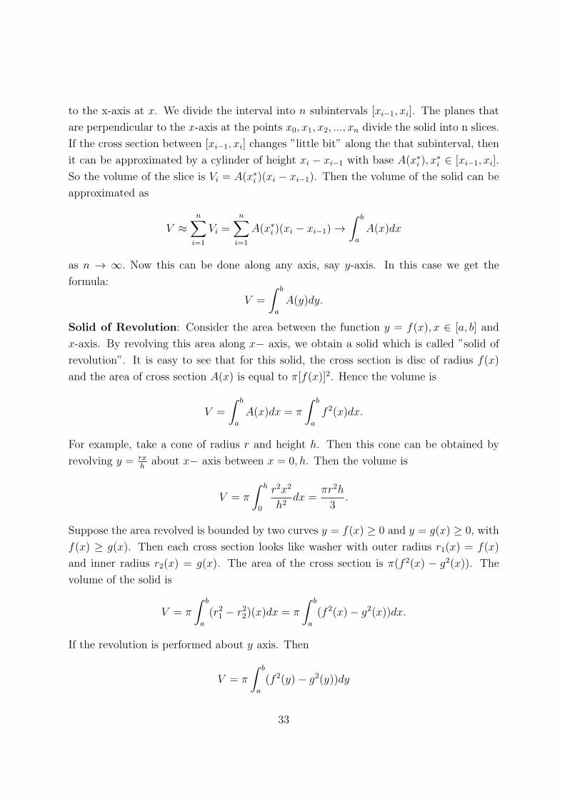
to the x-axis at x. We divide the interval into n subintervals [xi−1, xi]. The planes that

are perpendicular to the x-axis at the points x0, x1, x2, ..., xn divide the solid into n slices.

If the cross section between [xi−1, xi] changes ”little bit” along the that subinterval, then

it can be approximated by a cylinder of height xi − xi−1 with base A(x∗i ), x∗i ∈ [xi−1, xi].

So the volume of the slice is Vi = A(x∗i )(xi − xi−1). Then the volume of the solid can be

approximated as

V ≈n∑

i=1

Vi =n∑

i=1

A(x∗i )(xi − xi−1)→∫ b

a

A(x)dx

as n → ∞. Now this can be done along any axis, say y-axis. In this case we get the

formula:

V =

∫ b

a

A(y)dy.

Solid of Revolution: Consider the area between the function y = f(x), x ∈ [a, b] and

x-axis. By revolving this area along x− axis, we obtain a solid which is called ”solid of

revolution”. It is easy to see that for this solid, the cross section is disc of radius f(x)

and the area of cross section A(x) is equal to π[f(x)]2. Hence the volume is

V =

∫ b

a

A(x)dx = π

∫ b

a

f 2(x)dx.

For example, take a cone of radius r and height h. Then this cone can be obtained by

revolving y = rxhabout x− axis between x = 0, h. Then the volume is

V = π

∫ h

0

r2x2

h2dx =

πr2h

3.

Suppose the area revolved is bounded by two curves y = f(x) ≥ 0 and y = g(x) ≥ 0, with

f(x) ≥ g(x). Then each cross section looks like washer with outer radius r1(x) = f(x)

and inner radius r2(x) = g(x). The area of the cross section is π(f 2(x) − g2(x)). The

volume of the solid is

V = π

∫ b

a

(r21 − r22)(x)dx = π

∫ b

a

(f 2(x)− g2(x))dx.

If the revolution is performed about y axis. Then

V = π

∫ b

a

(f 2(y)− g2(y))dy

33

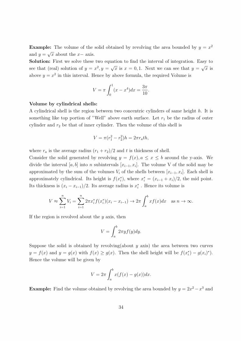
Example: The volume of the solid obtained by revolving the area bounded by y = x2

and y =√x about the x− axis.

Solution: First we solve these two equation to find the interval of integration. Easy to

see that (real) solution of y = x2, y =√x is x = 0, 1. Next we can see that y =

√x is

above y = x2 in this interval. Hence by above formula, the required Volume is

V = π

∫ 1

0

(x− x4)dx =3π

10.

Volume by cylindrical shells:

A cylindrical shell is the region between two concentric cylinders of same height h. It is

something like top portion of ”Well” above earth surface. Let r1 be the radius of outer

cylinder and r2 be that of inner cylinder. Then the volume of this shell is

V = π(r21 − r22)h = 2πrath,

where ra is the average radius (r1 + r2)/2 and t is thickness of shell.

Consider the solid generated by revolving y = f(x), a ≤ x ≤ b around the y-axis. We

divide the interval [a, b] into n subintervals [xi−1, xi]. The volume V of the solid may be

approximated by the sum of the volumes Vi of the shells between [xi−1, xi]. Each shell is

approximately cylindrical. Its height is f(x∗i ), where x∗i = (xi−1 + xi)/2, the mid point.

Its thickness is (xi − xi−1)/2. Its average radius is x∗i . Hence its volume is

V ≈n∑

i=1

Vi =n∑

i=1

2πx∗i f(x∗i )(xi − xi−1)→ 2π

∫ b

a

xf(x)dx as n→∞.

If the region is revolved about the y axis, then

V =

∫ b

a

2πyf(y)dy.

Suppose the solid is obtained by revolving(about y axis) the area between two curves

y = f(x) and y = g(x) with f(x) ≥ g(x). Then the shell height will be f(x∗i ) − g(xi)∗).

Hence the volume will be given by

V = 2π

∫ b

a

x(f(x)− g(x))dx.

Example: Find the volume obtained by revolving the area bounded by y = 2x2−x3 and

34

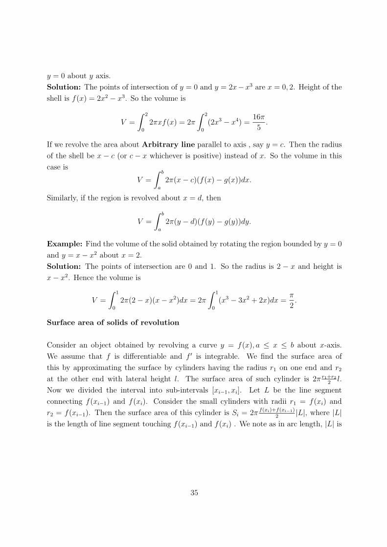
y = 0 about y axis.

Solution: The points of intersection of y = 0 and y = 2x−x3 are x = 0, 2. Height of the

shell is f(x) = 2x2 − x3. So the volume is

V =

∫ 2

0

2πxf(x) = 2π

∫ 2

0

(2x3 − x4) =16π

5.

If we revolve the area about Arbitrary line parallel to axis , say y = c. Then the radius

of the shell be x − c (or c − x whichever is positive) instead of x. So the volume in this

case is

V =

∫ b

a

2π(x− c)(f(x)− g(x))dx.

Similarly, if the region is revolved about x = d, then

V =

∫ b

a

2π(y − d)(f(y)− g(y))dy.

Example: Find the volume of the solid obtained by rotating the region bounded by y = 0

and y = x− x2 about x = 2.

Solution: The points of intersection are 0 and 1. So the radius is 2 − x and height is

x− x2. Hence the volume is

V =

∫ 1

0

2π(2− x)(x− x2)dx = 2π

∫ 1

0

(x3 − 3x2 + 2x)dx =π

2.

Surface area of solids of revolution

Consider an object obtained by revolving a curve y = f(x), a ≤ x ≤ b about x-axis.

We assume that f is differentiable and f ′ is integrable. We find the surface area of

this by approximating the surface by cylinders having the radius r1 on one end and r2

at the other end with lateral height l. The surface area of such cylinder is 2π r1+r22

l.

Now we divided the interval into sub-intervals [xi−1, xi]. Let L be the line segment

connecting f(xi−1) and f(xi). Consider the small cylinders with radii r1 = f(xi) and

r2 = f(xi−1). Then the surface area of this cylinder is Si = 2π f(xi)+f(xi−1)2

|L|, where |L|is the length of line segment touching f(xi−1) and f(xi) . We note as in arc length, |L| is

35

√1 +

(f(xi−1)−f(xi)

xi−xi−1

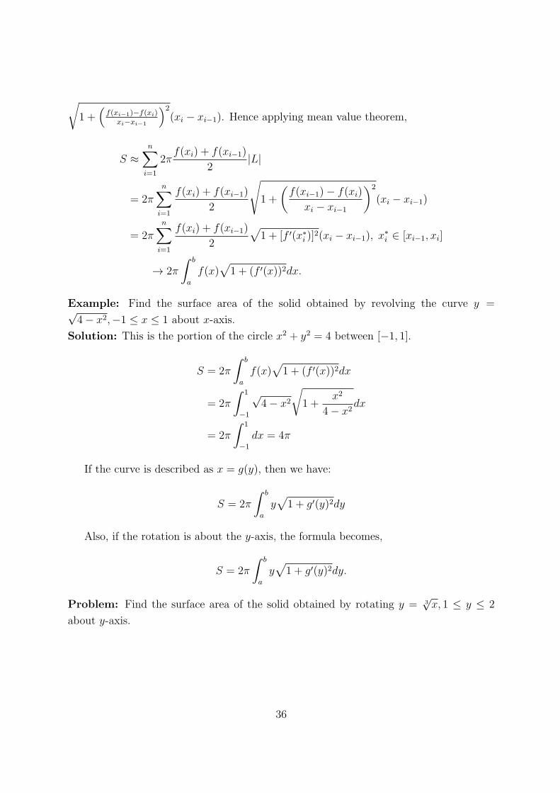
)2(xi − xi−1). Hence applying mean value theorem,

S ≈n∑

i=1

2πf(xi) + f(xi−1)

2|L|

= 2πn∑

i=1

f(xi) + f(xi−1)2

√1 +

(f(xi−1)− f(xi)

xi − xi−1

)2

(xi − xi−1)

= 2πn∑

i=1

f(xi) + f(xi−1)2

√1 + [f ′(x∗i )]2(xi − xi−1), x∗i ∈ [xi−1, xi]

→ 2π

∫ b

a

f(x)√1 + (f ′(x))2dx.

Example: Find the surface area of the solid obtained by revolving the curve y =√4− x2,−1 ≤ x ≤ 1 about x-axis.

Solution: This is the portion of the circle x2 + y2 = 4 between [−1, 1].

S = 2π

∫ b

a

f(x)√1 + (f ′(x))2dx

= 2π

∫ 1

−1

√4− x2

√1 +

x2

4− x2dx

= 2π

∫ 1

−1dx = 4π

If the curve is described as x = g(y), then we have:

S = 2π

∫ b

a

y√1 + g′(y)2dy

Also, if the rotation is about the y-axis, the formula becomes,

S = 2π

∫ b

a

y√1 + g′(y)2dy.

Problem: Find the surface area of the solid obtained by rotating y = 3√x, 1 ≤ y ≤ 2

about y-axis.

36

Solution: Given curve is x = y3, 1 ≤ y ≤ 2. By the given formula,

S = 2π

∫ 2

y=1

y3

√1 + (

dx

dy)2dy = 2π

∫ 2

1

y3√1 + 9y4dy

=2π

36

∫ 2

1

36y3√1 + 9y4dy =

π

27(1 + 9y4)3/22y=1 =

π

27(1453/2 − 103/2)

Problem: Find the surface area and volume of the solid generated by infinite curve

y = 1x, x ≥ 1. Interpret the result.

Solution: The surface area and volume are given by

S = 2π

∫ ∞

1

1

x

√1 +

1

x4dx, V = π

∫ ∞

1

1

x2dx

It is easy to see that the integral in S diverges. Indeed,

∫ b

1

1

x

√1 +

1

x4dx >

∫ b

1

1

xdx.

However, the integral for V converges. This is sometimes described as a can that does not

hold enough paint to cover its own interior. Of course, a finite amount of paint cannot

cover infinite surface. But if we fill the can with finite amount of paint we will have

covered an infinite surface. This is known as Painter’s paradox.

References

[1] Methods of Real Analysis, Chapter 2, R. Goldberg .

[2] Elementary Analysis: The Theory of Calculus, K. A. Ross.

[3] Understanding Analysis, Abbott,S.

[4] Calculus, G. B. Thomas and R. L. Finney, Pearson .

[5] Calculus, James Stewart, Brooks/Cole Cengage Learning.

37