Importance Sampling in Monte Carlo Simulation ofRare Transition Events∗

Wei Cai

Lecture 1. August 1, 2005

1 Motivation: time scale limit and rare events

Atomistic simulations such as Molecular Dynamics (MD) and Monte Carlo (MC) are playingan important role in our understanding of macroscopic behavior of materials in terms of theatomistic mechanisms. But the range of applicability of atomistic simulations is determinedby their limits of time and length scales, see Fig. 1. While the length scale limit of atomisticsimulations has been extended significantly through the use of massively parallel computing,the time scale limit is still a critical bottleneck to date.

Figure 1: Time and length scale limits of atomistic simulations.

∗Lecture notes and Matlab codes available at [1].

1

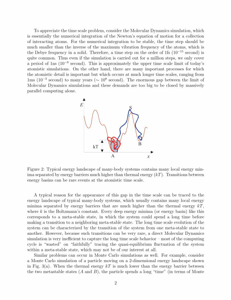
To appreciate the time scale problem, consider the Molecular Dynamics simulation, whichis essentially the numerical integration of the Newton’s equation of motion for a collectionof interacting atoms. For the numerical integration to be stable, the time step should bemuch smaller than the inverse of the maximum vibration frequency of the atoms, which isthe Debye frequency in a solid. Therefore, a time step on the order of 1fs (10−15 second) isquite common. Thus even if the simulation is carried out for a million steps, we only covera period of 1ns (10−9 second). This is approximately the upper time scale limit of today’satomistic simulations. On the other hand, there are many important processes for whichthe atomistic detail is important but which occurs at much longer time scales, ranging from1ms (10−3 second) to many years (∼ 108 second). The enormous gap between the limit ofMolecular Dynamics simulations and these demands are too big to be closed by massivelyparallel computing alone.

A

B

S E

x

kT

Figure 2: Typical energy landscape of many-body systems contains many local energy min-ima separated by energy barriers much higher than thermal energy (kT ). Transitions betweenenergy basins can be rare events at the atomistic time scale.

A typical reason for the appearance of this gap in the time scale can be traced to theenergy landscape of typical many-body systems, which usually contains many local energyminima separated by energy barriers that are much higher than the thermal energy kT ,where k is the Boltzmann’s constant. Every deep energy minima (or energy basin) like thiscorresponds to a meta-stable state, in which the system could spend a long time beforemaking a transition to a neighboring meta-stable state. The long time scale evolution of thesystem can be characterized by the transition of the system from one meta-stable state toanother. However, because such transitions can be very rare, a direct Molecular Dynamicssimulation is very inefficient to capture the long time scale behavior – most of the computingcycle is “wasted” on “faithfully” tracing the quasi-equilibrium fluctuation of the systemwithin a meta-stable state, which may not be of our interest at all.

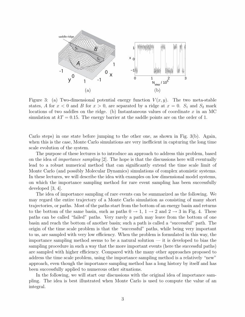
Similar problems can occur in Monte Carlo simulations as well. For example, considera Monte Carlo simulation of a particle moving on a 2-dimensional energy landscape shownin Fig. 3(a). When the thermal energy kT is much lower than the energy barrier betweenthe two metastable states (A and B), the particle spends a long “time” (in terms of Monte

2

0 1 2 3

−1

0

1

Nstep

/ 105

x

(a) (b)

Figure 3: (a) Two-dimensional potential energy function V (x, y). The two meta-stablestates, A for x < 0 and B for x > 0, are separated by a ridge at x = 0. S1 and S2 marklocations of two saddles on the ridge. (b) Instantaneous values of coordinate x in an MCsimulation at kT = 0.15. The energy barrier at the saddle points are on the order of 1.

Carlo steps) in one state before jumping to the other one, as shown in Fig. 3(b). Again,when this is the case, Monte Carlo simulations are very inefficient in capturing the long timescale evolution of the system.

The purpose of these lectures is to introduce an approach to address this problem, basedon the idea of importance sampling [2]. The hope is that the discussions here will eventuallylead to a robust numerical method that can significantly extend the time scale limit ofMonte Carlo (and possibly Molecular Dynamics) simulations of complex atomistic systems.In these lectures, we will describe the idea with examples on low dimensional model systems,on which the importance sampling method for rare event sampling has been successfullydeveloped [3, 4].

The idea of importance sampling of rare events can be summarized as the following. Wemay regard the entire trajectory of a Monte Carlo simulation as consisting of many shorttrajectories, or paths. Most of the paths start from the bottom of an energy basin and returnsto the bottom of the same basin, such as paths 0 → 1, 1 → 2 and 2 → 3 in Fig. 4. Thesepaths can be called “failed” paths. Very rarely a path may leave from the bottom of onebasin and reach the bottom of another basin; such a path is called a “successful” path. Theorigin of the time scale problem is that the “successful” paths, while being very importantto us, are sampled with very low efficiency. When the problem is formulated in this way, theimportance sampling method seems to be a natural solution — it is developed to bias thesampling procedure in such a way that the more important events (here the successful paths)are sampled with higher efficiency. Compared with the many other approaches proposed toaddress the time scale problem, using the importance sampling method is a relatively “new”approach, even though the importance sampling method has a long history by itself and hasbeen successfully applied to numerous other situations.

In the following, we will start our discussions with the original idea of importance sam-pling. The idea is best illustrated when Monte Carlo is used to compute the value of anintegral.

3

Figure 4: Schematic representation of a reactive trajectory in an energy landscape withmeta-stable states A and B. Such a trajectory can be sliced into a sequence of “failed”paths followed by a single “successful” path. A failed path is defined as a sequence ofmicrostates that initiates in region A, exits it at some instant, but returns to it beforereaching B. In contrast, a successful segment is defined as a sequence of states that initiatesin A and succeeds in reaching B before returning to state A. The shown reactive trajectoryconsists of three failed paths, namely, the sequences of states 0 → 1, 1 → 2, and 2 → 3, andthe successful path 3 → 4.

2 Monte Carlo computation of integrals

Very often, the purpose of a Monte Carlo simulation can be reformulated as for computingthe value of an integral. A typical example is to use Monte Carlo to evaluate the canonicalensemble average of a certain quantity, which may be expressed as a function of the positionsof all atoms, e.g. A(ri). The ensemble average of A is,

〈A〉 =1

Q

∫ N∏i=1

driA(ri) exp

[−V (ri)

kT

](1)

where

Q =

∫ N∏i=1

dri exp

[−V (ri)

kT

](2)

and N is the total number of atoms, V is the potential energy function, k is the Boltzmann’sconstant and T is the temperature. For large N , the dimension of the integral is too largeto be carried out by numerical quadrature. Monte Carlo is a convenient method to evaluatethis integral. By sampling a sequence of configurations, ri(m), m = 1, · · · ,M , that satisfiesthe probability distribution,

f(ri) =1

Qexp

[−V (ri)

kT

](3)

4

the ensemble average can be estimated from the numerical average [5],

〈A〉MC =1

M

M∑m=1

A(ri(m)) (4)

Contrary to the claims in [6], Eq. (4) is not importance sampling. As discussed below, we callsomething importance sampling if an importance function is introduced to further reducethe variance in the sampling.

2.1 One dimensional integral

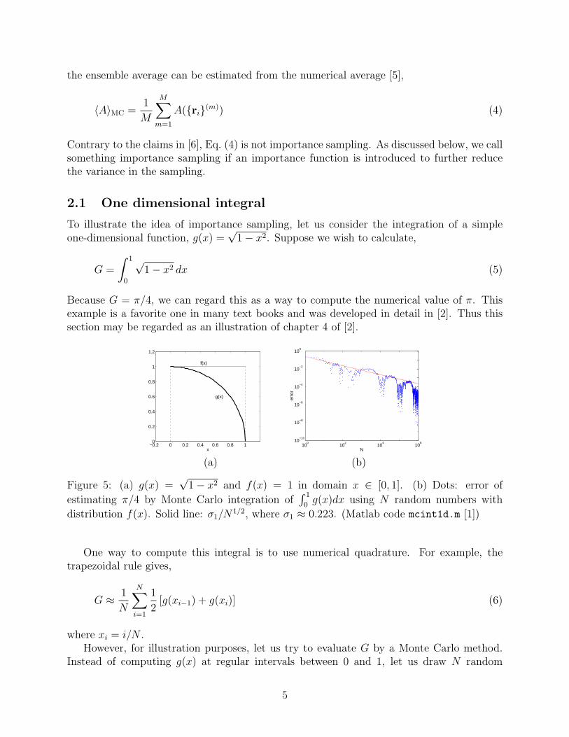
To illustrate the idea of importance sampling, let us consider the integration of a simpleone-dimensional function, g(x) =

√1− x2. Suppose we wish to calculate,

G =

∫ 1

0

√1− x2 dx (5)

Because G = π/4, we can regard this as a way to compute the numerical value of π. Thisexample is a favorite one in many text books and was developed in detail in [2]. Thus thissection may be regarded as an illustration of chapter 4 of [2].

−0.2 0 0.2 0.4 0.6 0.8 10

0.2

0.4

0.6

0.8

1

1.2

x

g(x)

f(x)

100

102

104

106

10−10

10−8

10−6

10−4

10−2

100

N

erro

r

(a) (b)

Figure 5: (a) g(x) =√

1− x2 and f(x) = 1 in domain x ∈ [0, 1]. (b) Dots: error of

estimating π/4 by Monte Carlo integration of∫ 1

0g(x)dx using N random numbers with

distribution f(x). Solid line: σ1/N1/2, where σ1 ≈ 0.223. (Matlab code mcint1d.m [1])

One way to compute this integral is to use numerical quadrature. For example, thetrapezoidal rule gives,

G ≈ 1

N

N∑i=1

1

2[g(xi−1) + g(xi)] (6)

where xi = i/N .However, for illustration purposes, let us try to evaluate G by a Monte Carlo method.

Instead of computing g(x) at regular intervals between 0 and 1, let us draw N random

5

numbers xi, i = 1, · · · , N that are independently and uniformly distributed in [0, 1]. Let GN

be the average of these random numbers,

GN =1

N

N∑i=1

g(xi) (7)

Notice that GN is a random number itself. The expectation value of GN is G, i.e.,

G = 〈GN〉 (8)

Mathematically, this means we rewrite G as,

G =

∫g(x)f(x) dx = 〈g〉f (9)

where f(x) is the distribution density function of the random variables, f(x) = 1 if 0 ≤ x ≤ 1and f(x) = 0 otherwise. In other words, G is the average of function g(x) under distributionf(x). The variance of GN is

varGN =σ2

1

N(10)

where

varg = σ21 =

∫g2(x)f(x) dx−G2 (11)

The error of GN in estimating G is comparable to the standard deviation of GN , i.e.

error = ε ≈ σ1

N1/2(12)

In this example, σ21 = 2/3− (π/4)2 ≈ 0.0498, σ1 ≈ 0.223. According to Eq. (12), we expect

the error, |GN − π/4|, should decay as 0.223/N1/2 as the number N of random variablesincrease. This is confirmed by numerical results, as shown in Fig. 5(b).

2.2 Importance sampling in Monte Carlo integration

Using a uniform distribution function f(x) is not necessarily the optimal way of doing MonteCarlo integration, in the sense that it does not necessarily give the smallest statistical fluc-tuation, i.e. varGN.

Imagine that we use random variables that satisfy another density distribution function,f(x). Then the integral can be rewritten as,

G =

∫ [f(x)g(x)

f(x)

]f(x) dx ≡

∫g(x)f(x) dx = 〈g〉f (13)

This means that G is also the expectation value of g(x) ≡ f(x)g(x)/f(x) under distributionfunction f(x). The variance of this estimator is,

varg =

∫g2(x)f(x) dx−G2 =

∫ [f(x)g(x)

f(x)

]2

f(x) dx−G2 =

∫f 2(x)g2(x)

f(x)dx−G2 (14)

6

To illustrate that different distribution functions give rise to different variance, considera family of f(x),

f(x) =

(1− βx2)/(1− β/3), 0 ≤ x ≤ 10, otherwise

(15)

Notice that when β = 0, f(x) corresponds to the uniform distribution considered above.Fig. 6(a) shows the numerical error of GN (compared with π/4) as a function of N

(number of random variables) for β = 0 and β = 0.74. The error is systematically lower inthe β = 0.74 case, which scales as 0.054/N1/2. The variance of g under distribution functionf can be obtained analytically [2],

varg =

(1− β

3

) [1

β− 1− β

β3/2tanh−1 β1/2

]−

(π4

)2

(16)

It is plotted in Fig. 6(b). The variance reaches a minimum at β ≈ 0.74. This means that,among the family of importance functions given in Eq. (15), the one with Eq. (15) is the(local) optimal.

100

102

104

106

10−8

10−6

10−4

10−2

100

N

erro

r

β=0.74

β=0

0 0.2 0.4 0.6 0.8 10

0.01

0.02

0.03

0.04

0.05

β

var

g

Figure 6: (a) Error of Monte Carlo integration as a function of N , the number of randomvariables which are distributed according to f(x) = (1 − βx2)/(1 − β/3). (b) Variation ofg(x) as a function of β. (Matlab code mcint1d imp.m [1])

Exercise: for f(x) = (1 − βx)/(1 − β/2), derive varg and the optimal value of β. Plotnumerical error of 〈g〉f as a function of N (as in Fig. 6(a)) for β = 0 and the (local) optimalvalue of β.

What is the optimal importance function f among all possible functions? To answerthis question, we should minimize varg with respect to f under the constraint that∫f(x)dx = 1, f(x) ≥ 0 (because f is a probability distribution function). Introduce La-

grangian multiplier λ, we wish to minimize a functional [2],

Lf =

∫f 2(x)g2(x)

f(x)+ λf(x) dx (17)

At the minimum,

δL

δf= −f

2(x)g2(x)

f 2(x)+ λ = 0 (18)

7

Hence,

f(x) = λ|g(x)f(x)| (19)

The normalization condition of f(x) demands that λ = 1/G, so that the (global) optimalimportance function is,

f(x) =1

G|g(x)f(x)| (20)

Notice that when the (global) optimal importance function is used,

g(x) = Gf(x)g(x)

|f(x)g(x)|(21)

If g(x) is non-negative, this means that g(x) is a constant, and equals G. Therefore, when the(global) optimal importance function is used, the statistical variance is zero, because everyrandom number gives identical contribution to the integral. This finding is not surprisingbecause whenever g(x) is not a constant, there is always a finite variance when computingits average. Zero variance is reached if and only if g(x) is a constant.

Unfortunately, the (global) optimal importance function contains the information of theanswer we were after (G) in the first place. This means finding the (global) optimal impor-tance function is not easier than finding the integral G itself. Thus for practical purposes,we need to assume that we do not have the (global) optimal importance function when wecompute G. Fortunately, even if f is not the (global) optimum, it can still reduce the sta-tistical variance of the estimate of G. The closer f is to the (global) optimum, the smallerthe variance becomes. Therefore, the importance sampling method is usually accompaniedby the effort to improve the importance function.

3 Random walks, differential and integral equations

Usually, Monte Carlo simulations use a Markov process to generate a sequence of randomvariables to be used in the numerical integration. In this case, the system may be regardedas doing random walks in the phase space. We have already seen the connection betweenthe Monte Carlo method and integrals. This is closely related to the (probably even deeper)connection between random walks and integral equations [2, 8, 9] and partial differentialequations (PDEs) [7].

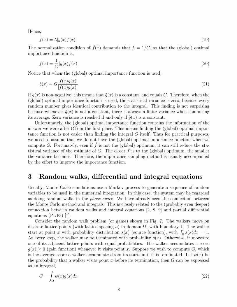
Consider the random walk problem (or game) shown in Fig. 7. The walkers move ondiscrete lattice points (with lattice spacing a) in domain Ω, with boundary Γ. The walkerstart at point x with probability distribution s(x) (source function), with

∫Ωs(x)dx = 1.

At every step, the walker may be terminated with probability q(x). Otherwise, it moves toone of its adjacent lattice points with equal probabilities. The walker accumulates a scoreg(x) ≥ 0 (gain function) whenever it visits point x. Suppose we wish to compute G, whichis the average score a walker accumulates from its start until it is terminated. Let ψ(x) bethe probability that a walker visits point x before its termination, then G can be expressedas an integral,

G =

∫Ω

ψ(x)g(x)dx (22)

8

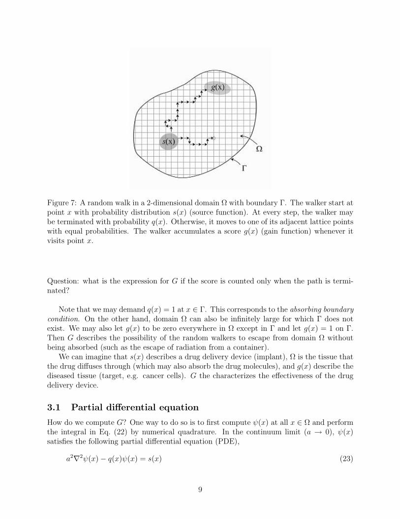
Figure 7: A random walk in a 2-dimensional domain Ω with boundary Γ. The walker start atpoint x with probability distribution s(x) (source function). At every step, the walker maybe terminated with probability q(x). Otherwise, it moves to one of its adjacent lattice pointswith equal probabilities. The walker accumulates a score g(x) (gain function) whenever itvisits point x.

Question: what is the expression for G if the score is counted only when the path is termi-nated?

Note that we may demand q(x) = 1 at x ∈ Γ. This corresponds to the absorbing boundarycondition. On the other hand, domain Ω can also be infinitely large for which Γ does notexist. We may also let g(x) to be zero everywhere in Ω except in Γ and let g(x) = 1 on Γ.Then G describes the possibility of the random walkers to escape from domain Ω withoutbeing absorbed (such as the escape of radiation from a container).

We can imagine that s(x) describes a drug delivery device (implant), Ω is the tissue thatthe drug diffuses through (which may also absorb the drug molecules), and g(x) describe thediseased tissue (target, e.g. cancer cells). G the characterizes the effectiveness of the drugdelivery device.

3.1 Partial differential equation

How do we compute G? One way to do so is to first compute ψ(x) at all x ∈ Ω and performthe integral in Eq. (22) by numerical quadrature. In the continuum limit (a → 0), ψ(x)satisfies the following partial differential equation (PDE),

a2∇2ψ(x)− q(x)ψ(x) = s(x) (23)

9

This is simply a absorption-diffusion equation. The problem with this approach is that, itcan be very wasteful since we only want to know the value of G, which is a weighted integralof ψ(x). Yet we obtained ψ(x) at every point x in Ω. For example, g(x) may be non-zeroonly in a small region of Ω. Hence, in principle, we do not need to know ψ(x) in the restregion of Ω. Ω may also be infinite, in which case it may not be possible to store values ofψ(x) everywhere in Ω.

3.2 Monte Carlo simulation

Another approach is to perform Monte Carlo simulation of the random walkers according tothe prescribed rules, and estimate G by averaging the gain function g(x) over the locationswhere the walkers have visited. Suppose we initiate N walkers, then

GN =1

N

N∑n=1

∑i

g(x(n)i ) (24)

is an estimate of G, where x(m)i is the location of walker m at step i. The potential problem

of this approach is that the efficiency may be very low, if the majority of the walkers do notvisit regions where g(x) > 0.

For example, consider the case when g(x) = 1 in a small region of Ω that is separatedfrom the region where s(x) = 1 and that the termination rate q(x) is high compared in theentire domain Ω. Also assume that q(x) = 1 at locations where g(x) = 1, i.e. the walkersterminate immediately after it scores (but the majority of the walkers terminate at g(x) = 0,i.e. without score). Let p be the probability that the walker makes a non-zero contribution(g(x) = 1) to the total score G, then,

G = 〈GN〉 = p (25)

The variance of GN is,

varGN =p(1− p)

N(26)

so that the error in estimating G is approximately,

error = ε ≈ p1/2(1− p)1/2

N1/2(27)

In the limit of p 1,

ε ≈ p1/2

N1/2(28)

and the relative error is,

ε

G≈ 1

(pN)1/2(29)

Thus we obtain meaningful results only if N 1/p. For example, if p ∼ 10−6, the N needsto be 108 to achieve a relative error of 1%.

10

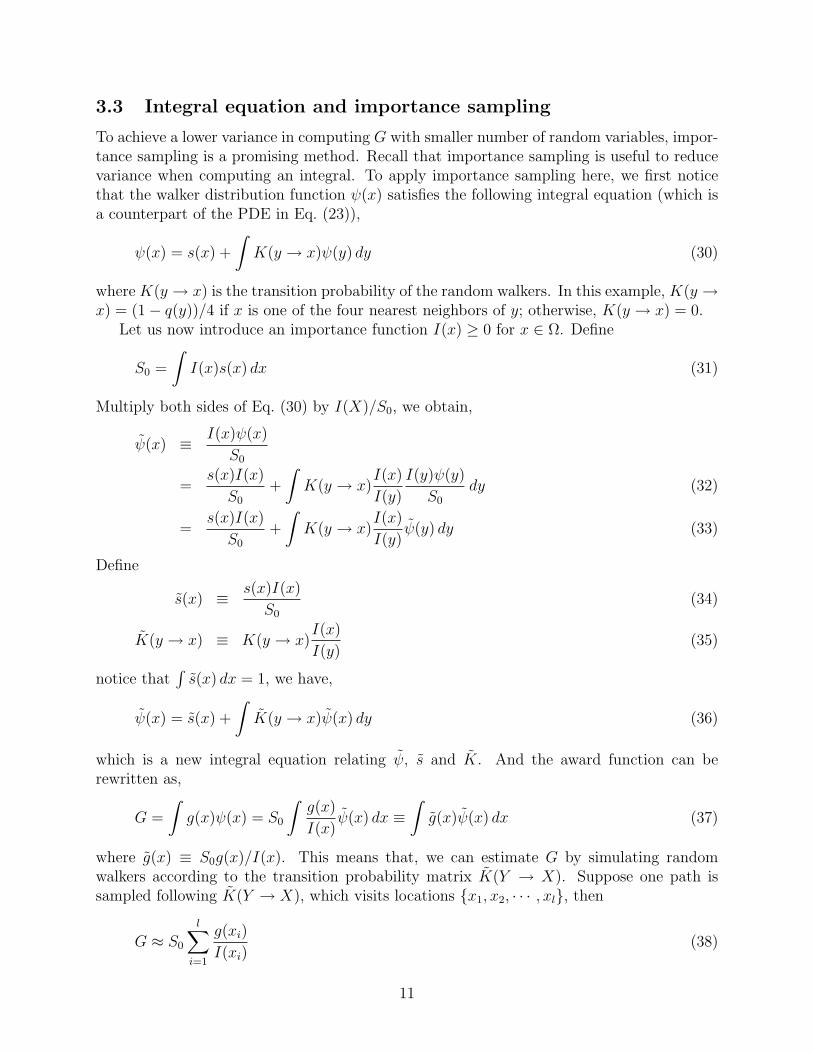
3.3 Integral equation and importance sampling

To achieve a lower variance in computing G with smaller number of random variables, impor-tance sampling is a promising method. Recall that importance sampling is useful to reducevariance when computing an integral. To apply importance sampling here, we first noticethat the walker distribution function ψ(x) satisfies the following integral equation (which isa counterpart of the PDE in Eq. (23)),

ψ(x) = s(x) +

∫K(y → x)ψ(y) dy (30)

where K(y → x) is the transition probability of the random walkers. In this example, K(y →x) = (1− q(y))/4 if x is one of the four nearest neighbors of y; otherwise, K(y → x) = 0.

Let us now introduce an importance function I(x) ≥ 0 for x ∈ Ω. Define

S0 =

∫I(x)s(x) dx (31)

Multiply both sides of Eq. (30) by I(X)/S0, we obtain,

ψ(x) ≡ I(x)ψ(x)

S0

=s(x)I(x)

S0

+

∫K(y → x)

I(x)

I(y)

I(y)ψ(y)

S0

dy (32)

=s(x)I(x)

S0

+

∫K(y → x)

I(x)

I(y)ψ(y) dy (33)

Define

s(x) ≡ s(x)I(x)

S0

(34)

K(y → x) ≡ K(y → x)I(x)

I(y)(35)

notice that∫s(x) dx = 1, we have,

ψ(x) = s(x) +

∫K(y → x)ψ(x) dy (36)

which is a new integral equation relating ψ, s and K. And the award function can berewritten as,

G =

∫g(x)ψ(x) = S0

∫g(x)

I(x)ψ(x) dx ≡

∫g(x)ψ(x) dx (37)

where g(x) ≡ S0g(x)/I(x). This means that, we can estimate G by simulating randomwalkers according to the transition probability matrix K(Y → X). Suppose one path issampled following K(Y → X), which visits locations x1, x2, · · · , xl, then

G ≈ S0

l∑i=1

g(xi)

I(xi)(38)

11

0 10 20 30 400

5

10

15

20

25

30

35

40

x

y

010

2030

40

0

20

400

0.5

1

1.5

2

xy

ψ

(a) (b)

0 1 2 3 40.04

0.045

0.05

0.055

µ

G

0 1 2 3 40

0.5

1

1.5

2

2.5

3x 10

−3

µ

erro

r

(c) (d)

Figure 8: (a) Random walk is within the (red) rectangle on a square lattice with spacinga = 1. The source function s(x) equals 1 at the circle and zero everywhere else. The contourline of ψ(x) in (b) is also plotted. (b) The density distribution ψ(x) from 1000 randomwalkers. (c) Estimates of G using importance functions with different parameter µ. (d)Standard deviation of estimates in (c) as a function of µ.

12

In the new random walk, the walker distribution density is ψ(x). The variance is reduced ifthere is a significant overlap between regions where ψ(x) > 0 and g(x) > 0.

To give a specific example, consider a rectangular domain shown in Fig. 8(a). The sourcefunction s(x) equals 1 at one point x0 (marked by the circle) and zero everywhere else. Thegain function g(x) = 0 and the termination probability q(x) = r (r = 0.05) everywhere insideΩ except at boundary Γ. At boundary Γ, g(x) = 1 and q(x) = 1. Thus G is the probabilityof the walkers escaping (reaching Γ) before being absorbed at the interior of Ω.

The distribution ψ(x) estimated from 1000 random walkers are plotted in Fig. 8(b). Wenotice that most of the walkers terminate at the interior of Ω. The estimated value from 104

walkers is G ≈ 4.84± 0.28× 10−2.Suppose we use the importance function of the following form,

I(x) = exp[−µ exp

(−α|x− x0|2

)](39)

Fig. 8(c) plots the estimate of G for different values of µ when α = 0.03 from 104 walkers.The standard deviation of these estimates are plotted in Fig. 8(d). We observed that µ ≈ 3is the optimal value giving rise to the lowest statistical error.

References

[1] More materials of these lectures are available athttp://micro.stanford.edu/∼caiwei/LLNL-CCMS-2005-Summer/

[2] M.H. Kalos and P. A. Whitlock, Monte Carlo Methods, Volume I: Basics, (Wiley, NewYork, 1986).

[3] W. Cai, M. H. Kalos, M. de Koning and V. V. Bulatov, Importance sampling of raretransition events in Markov processes, Phys. Rev. E 66, 046703 (2002).

[4] M. de Koning, W. Cai, B. Sadigh, T. Oppelstrup, M. H. Kalos, and V. V. Bulatov, Adap-tive importance sampling Monte Carlo simulation of rare transition events, J. Chem.Phys. 122, 074103 (2005).

[5] D. Frenkel and B. Smit, Understanding Molecular Simulations: from Algorithms toApplications, (Academic Press, San Diego, 2002).

[6] M. P. Allen and D. J. Tildesley, Computer Simulation of Liquids, (Oxford UniversityPress, 1987).

[7] L. C. Evans, An Introduction to Stochastic Differential Equations, Department of Math-ematics, UC Berkeley, http://math.berkeley.edu/ evans/SDE.course.pdf.

[8] R. P. Feynman, The Principle of Least Action in Quantum Mechanics, Ph.D. Thesis,Princeton University, May, 1942.

[9] B. Dynkin and A. A. Yshkevich, Markov Processes: Theorems and Problems, (PlenumPress, New York, 1969).

13

Importance Sampling in Monte Carlo Simulation ofRare Transition Events∗

Wei Cai

Lecture 2. August 2, 2005

0 10 20 30 400

5

10

15

20

25

30

35

40

x

y

010

2030

40

0

20

400

0.5

1

1.5

2

xy

ψ

(a) (b)

010

2030

40

0

20

40−3

−2

−1

0

xy

log 10

J

(c)

Figure 1: (a) Contour line of the exact solution of the walker density distribution func-tion ψ(x), which satisfies the integral equation, ψ(x) = s(x) +

∫ψ(y)K(y → x) dy.

G =∫ψ(x)g(x) dx = 4.6844 × 10−2. (diffuse2d exact sol.m) (b) 3D plot of ψ(x).

(c) Exact solution of the optimal importance function J(x), which satisfies the integralequation, J(x) = g(x) +

∫K(x → y)J(y) dy. G =

∫J(x)s(x) dx = 4.6844 × 10−2.

(diffuse2d opt imp.m)

∗Notes and Matlab codes available at http://micro.stanford.edu/∼caiwei/LLNL-CCMS-2005-Summer/

1

1-b

b

Importance Sampling in Monte Carlo Simulation ofRare Transition Events∗

Wei Cai

Lecture 3. August 3, 2005

−2−1

01

2

−2

0

2−1

0

1

2

3

xy

E

−1.5 −1 −0.5 0 0.5 1 1.5−1.5

−1

−0.5

0

0.5

1

1.5

x

y

(a) (b)

−2 −1 0 1 2−2

−1

0

1

2−15

−10

−5

0

x

y

ψ

−2

0

2

−2

0

2−15

−10

−5

0

xy

log 10

J

(c) (d)

Figure 1: (a)2D potential landscape. (b) Contour plot of (a). Circle: q(x) = 1, g(x) = 0.Cross: q(x) = 1, g(x) = 1. (c) Exact solution of walker density ψ(x). Average gainG =

∫ψ(x)g(x)dx = 2.7598 × 10−12. (d) Exact solution of optimal importance function

J(x, y). G =∫s(x)J(x)dx = 2.7598× 10−12. (pot2d exact sol.m)

∗Notes and Matlab codes available at http://micro.stanford.edu/∼caiwei/LLNL-CCMS-2005-Summer/

1