Institute of Parallel and Distributed SystemsUniversity of StuttgartUniversitätsstraße 38D–7 05 69 Stuttgart

Diplomarbeit Nr. 32 68

Implementierung einesPeridynamik–Verfahrens auf GPU

Patrick Diehl

Course of Study: Software Engineering

Examiner: Prof. Dr. Marc Alexander Schweitzer

Supervisor: M. Sc. Sa Wu

Commenced: November 14 2011

Completed: May 15 2012

CR-Classification: J.2, G.4

A computer will do what you tell itto do, but that may be much differ-ent from what you had in mind.

(Joseph Weizenbaum)

Contents

1 Introduction 1

2 Related work 3

3 Peridynamics 5

3.1 Peridynamic theory . . . . . . . . . . . . . . . . . . . . . . . . . . . . . . . 5

3.2 Inner forces for the Peridynamic theory . . . . . . . . . . . . . . . . . . . 8

3.2.1 Prototype Microelastic Brittle Model . . . . . . . . . . . . . . . . . 8

3.2.2 Short range forces . . . . . . . . . . . . . . . . . . . . . . . . . . . 9

3.3 Discretization . . . . . . . . . . . . . . . . . . . . . . . . . . . . . . . . . . 10

3.3.1 Computation of the position at time t . . . . . . . . . . . . . . . . 12

4 Implementation 13

4.1 Compute Unified Device Architecture . . . . . . . . . . . . . . . . . . . . 13

4.2 Program flow . . . . . . . . . . . . . . . . . . . . . . . . . . . . . . . . . . 16

4.2.1 Neighborhood search . . . . . . . . . . . . . . . . . . . . . . . . . 17

4.2.2 Update Positions . . . . . . . . . . . . . . . . . . . . . . . . . . . . 18

4.2.2.1 Parallelization of the discrete Peridynamic equation ofmotion . . . . . . . . . . . . . . . . . . . . . . . . . . . . 19

4.2.2.2 Maximal amount of particles . . . . . . . . . . . . . . . . 20

4.3 Measurement of the computation time . . . . . . . . . . . . . . . . . . . . 22

4.4 Challenges with the Compute Unified Device Architecture . . . . . . . . 23

5 Combination with the Partition of Unity Method 27

6 Results 29

6.1 Experiment 1 . . . . . . . . . . . . . . . . . . . . . . . . . . . . . . . . . . 29

6.2 Experiment 2 . . . . . . . . . . . . . . . . . . . . . . . . . . . . . . . . . . 37

7 Conclusion and outlook 45

Index vii

Bibliography vii

i

List of Symbols

αThe scaling parameter in the Prototype Microelastic Brittle material.

cThe stiffness constant in the Prototype Microelastic Brittle model in kg

m3 .

δThe radius of the horizon of a particle P in m.

ηThe relative displacement of two particles Pi and Pj.

HiThe horizon of a particle Pi.

kThe bulk modulus in the Prototype Microelastic Brittle material in GPa.

ΩThe reference configuration of the body.

RThe body.

ρ

The mass density of the material in the reference configuration Ω in kgm3 .

rsThe radius of a particle in m.

s00The critical stretch for bond failure for the Prototype Microelastic Brittle material.

ii

VThe volume of a particle in m3.

xThe initial position of a particle P relating to the reference configuration Ω.

ξThe relative position of two particles Pi and Pj in the reference configuration Ω.

iii

List of Figures

3.1 Body R with particles P1···n and the horizon Hi of particle Pi. . . . . . . 6

3.2 Bond force in the PMB model visualized as a function f (s). . . . . . . . 9

3.3 Discretization of the body R in N particles on an equidistant n × mlattice. . . . . . . . . . . . . . . . . . . . . . . . . . . . . . . . . . . . . . . . 10

4.1 Processing flow on CUDA . . . . . . . . . . . . . . . . . . . . . . . . . . . 14

4.2 Layers of CUDA . . . . . . . . . . . . . . . . . . . . . . . . . . . . . . . . . 14

4.3 Memory access model of CUDA . . . . . . . . . . . . . . . . . . . . . . . 16

4.4 Program flow chart of the simulation. . . . . . . . . . . . . . . . . . . . . 17

4.5 Example of morton order / z order. . . . . . . . . . . . . . . . . . . . . . 18

4.6 Run time of the STANN library on a equidistant two dimensional lattice. 19

4.7 Data structures on the CUDA device. . . . . . . . . . . . . . . . . . . . . 20

4.8 Run time of the different implementations for one particle per time step. 23

4.9 Run time with and without the update of neighbors step. . . . . . . . . 24

4.10 Global memory and caching . . . . . . . . . . . . . . . . . . . . . . . . . . 25

5.1 Combination with the Partition of Unity Method . . . . . . . . . . . . . 28

6.1 Blueprint and reference configuration Ω of the body R (experiment 1). 30

6.2 Forces on the horizontal edges (experiment 1). . . . . . . . . . . . . . . . 30

6.3 Growing of the crack (1µs–5µs) and delay of the crack (6µs–10µs) . . . . 36

6.4 Blueprint of the cylinder (experiment 2). . . . . . . . . . . . . . . . . . . 37

6.5 Model of the projectile (experiment 2). . . . . . . . . . . . . . . . . . . . . 37

6.6 Reference configuration and the impact of the projectile. . . . . . . . . . 39

6.7 Top layer of the body R during the impact. . . . . . . . . . . . . . . . . . 43

iv

List of Tables

6.1 Simulation parameters for experiment 1 . . . . . . . . . . . . . . . . . . . 31

6.2 Simulation parameters for experiment 2 . . . . . . . . . . . . . . . . . . . 38

List of Listings

4.1 The parallel computation of the equation of motion and the estimationof the new positions on the CUDA device . . . . . . . . . . . . . . . . . . 21

List of Acronyms

CUDA Compute Unified Device Architecture

CPU Central processing unit

FEM Finite Element Method

FLOPS Floating Point Operations Per Second

GPU Graphics processing unit

HPC High Performance Computing

MD Molecular Dynamics

MP Multiprocessor

v

MPI Message Passing Interface

OCL Open Computing Language

ODE Ordinary differential equation

PDE Partial differential equation

PMB Prototype Microelastic Brittle

PUM Partition of Unity Method

RAM Random-Access Memory

SIMT Single Instruction Multiple Threads

SPH Smoothed Particle Hydrodynamics

vi

1 Introduction

This thesis examines the use of the Compute Unified Device Architecture (CUDA) theimplementation of a Peridynamic technique on a Graphics processing unit (GPU).CUDA is a parallel computing architecture for NVIDIA GPUs. The NVIDIA GPUsare programmable through different industry standard programming languages.In this thesis the programming language “C for CUDA” is used to implement thePeridynamic technique. “C for CUDA” is similar to the programming language C withsome restrictions. The software was executed on a NVIDIA GeForce GTX 560 Ti.

The Peridynamic theory is a non local theory in continuum mechanic, with afocus on discontinuous functions as they arrive in fracture mechanics. The word“Peridynamic” is the syncrisis of the two Greek words πε$ι (peri = near) and δυναµη(dynami = force). The principle of this theory is that particles in a continuum interactwith other particles in a finite distance by exchanging forces.

Outline

The chapters cover following topics:

Chapter 2 – Related work: This chapter contains information about other implemen-tations of the Peridynamic technique, which use different kinds of massivelyparallel architectures.

Chapter 3 – Peridynamics: This chapter contains the basics of the Peridynamic andthe discrete Peridynamic equation of motion (equation 3.18).

Chapter 4 – Implementation: This chapter contains a short introduction to ComputeUnified Device Architecture (CUDA) and the program flow chart (figure 4.4) ofthe simulation. For each activity of the program flow chart the used algorithmsare introduced.

Chapter 5 – Combination with the Partition of Unity Method: This chapter containsan approach to the combination of the the Peridynamic technique with thePartition of Unity Method (PUM).

1

1 Introduction

Chapter 6 – Results: This chapter contains the results of two simulations: In the 2Dcase a thick square plate with a initial crack. In the 3D case the impact of aprojectile in a cylinder.

Chapter 7 – Conclusion and outlook: This chapter summarizes the results of this the-sis and gives an overview of potential improvements and features of the software.

2

2 Related work

“EMU is the first code based on the Peridynamic theory of solid mechanics”

According to the quote [Sana] EMU is the first implementation of the Peridynamictheory, which is implemented in FORTRAN 90 and provided from the Sandia NationalLaboratories. Developers implemented EMU variants to add extended features tothe standard version. In the aviation industry Dr. Abe Askari works on modeling offatigue cracks and composite material failure for Boeing Corporation.

In research Peridynamics PDLAMMPS and SIERRA/SM are the most commontools, which realizing the Peridynamic technique.Peridynamics PDLAMMPS [PSP+

11] is a realization of the Peridynamics in LAMMPS.LAMMPS [Pli95, Sanb] is a classical molecular dynamics code and the integrationof the Peridynamic technique is possible, because the Peridynamic technique is insome sections similar to a molecular dynamics (MD). Sierra/Solid Mechanics [SIE11] isbased on the Sierra Framework [Edw02] and provides a realization of the Peridynamictheory too. Because it is based on the Sierra Framework a coupling with other SIERRAmechanics codes is possible.

Nowadays most simulations are executed on massively parallel distributed sys-tems. Therefore frameworks like the Message Passing Interface (MPI) to distributedthe simulation on different Central processing units exist. It is possible to buildPDLAMMPS with MPI support.

Another approach for massively parallel programming is to execute the simula-tion on GPUs. For this exist Open Computing Language (OCL) and Compute UnifiedDevice Architecture (CUDA). This thesis studies the use of CUDA to realize amassively parallel implementation of the Peridynamic technique.

3

3 Peridynamics

The Peridynamic theory is a non local theory in continuum mechanics. As describedin [ELP] the Partial differential equation (PDE) (3.1) defines linear elastic behavior ofsolids, according to Newton’s second law: f orce = mass× acceleration.

$(x)∂2t u(x, t) = (Lu)(x, t) + b(x, t), (x, t) ∈ Ω× (0, T) (3.1)

with (Lu)(x, t) := (λ + µ) grad div u(x, t) + µ div grad u(x, t)

PDE (3.1) contains information about the material with $(x) as the density of the body.The inner tensions and macroscopic forces are described with the Lamé parametersµ and λ. The term b(x, t) defines the extern force at position x at time t. Thedisplacement field is described with u : Ω× [0, T] → Rd with d ∈ 1, 2, 3.

PDE (3.1) implies that the displacement of the body is twice continuously dif-ferentiable. With this assumption it is not possible to model cracks or fracture, becausea crack or fracture implies discontinuities in the displacement field u. Discontinuitiesconflict with the assumption that u is twice continuously differentiable.

An alternative theory to model solid mechanics is the Peridynamic theory, which wasintroduced by Silling [Sil00] in 2000. The Peridynamic theory formulates the problemwith an integro-differential equation. This solves the conflict of the discontinuities andthe twice continuously differentiability.

3.1 Peridynamic theory

The word “Peridynamic” is the syncrisis of the two Greek words πε$ι (peri = near)and δυναµη (dynami = force). The principle of this theory is that particles in acontinuum interact with other particles in a finite distance by exchanging forces. Someof this concepts are similar to a selection of a Molecular Dynamics (MD).

Figure 3.1 shows the body R in the reference configuration with particles P1···n.Each particle has a initial position x relating to the reference configuration Ω. To

5

3 Peridynamics

define which other particles interact with a particle each particle has a horizon Hiwith the radius δ. All other particles in this horizon Hi have a bond with the particlePi and interact with this particle by forces. Metaphorically speaking the particle doesnot “see” particles outside his own horizon Hi and is not influenced by them.

R

δ

ξ

x

x′

Hi

Figure 3.1: The body R of the continuum with particles P1···n andthe horizon Hi of particle Pi.

To compute the acceleration of a particle Pi in the reference configuration Ω at time tfollowing definitions are made:

ξ(t) = x′(0)− x(0) (3.2)

The relative position of two particles Pi and P′, with coordinates x and xi, in the

reference configuration Ω is defined as ξ(t).

η(t) = u(x′, t)− u(x, t) (3.3)

The relative displacement of two particles Pi and P′

is defined as η(t), withu(x, t) = x(t) − x(0). The current relative position is defined as η + ξ.

With this two definitions the acceleration of a particle Pi in the reference configurationΩ at time t is defined by the integral equation (3.4).

$(x)y(x, t) =∫

Hi

f ((u(x′, t)− u(x, t), x

′ − x)dVx′ + b(x, t) (3.4)

Equation (3.4) contains at the left hand side the function $(x). This function $(x)returns the mass density ρ of the material at position x in the reference configuration Ω.

6

3.1 Peridynamic theory

At the right side u is the displacement vector field, b(x, t) returns the external force atposition x at time t and f is the pairwise force function. The pairwise force functionf returns the force vector (per unit volume squared) which particle P

′exerts on the

particle Pi.For the horizon Hi exists, for a given material, a positive number δ such that:

|ξ| > δ ⇒ f (η, ξ) = 0 | ∀η (3.5)

This means that an spherical neighborhood Hi of particle Pi in R exists and thereare particles outside the neighborhood, which have no influence on particle P. Toassure the conservation of linear momentum p = m · v and angular momentumL = r× p = r×m · v the pairwise force function f is required to have the followingproperties:

∀η, ξ : f (−η,−ξ) = f (η, ξ) (3.6)

Property (3.6) assures the conservation of linear momentum, which means, that themomentum of the closed system is constant, if no external force acts on the closedsystem.

∀η, ξ : (η + ξ)× f (η, ξ) = 0 (3.7)

The property (3.7) assures the conversation of angular momentum. In closed systemsthe angular momentum is constant. The meaning of the equation (3.7) is, that the forcevector between particle Pi and P

′is parallel to their current relative position vector

η + ξ.For a micro elastic material the pairwise force function has to be derivable from ascalar micro potential w:

∀η, ξ : f (η, ξ) =∂w∂η

(η, ξ) (3.8)

The micro potential has the unit of energy per unit volume and holds the energyfor a single bond. A bond between a particle Pi and P

′exists, if particle P

′is in the

neighborhood Hi. The local strain energy density per unit volume in the body R isdefined as:

W =12

∫Hi

w(η, ξ)dVξ (3.9)

The factor 1/2 results because each particle of the bond holds half of the energy of thebond.

7

3 Peridynamics

3.2 Inner forces for the Peridynamic theory

In section 3.1 the theory of Peridynamic is described, but there is no description of thepairwise force function f . The subsection 3.2.1 gives a definition for a pairwise forcefunction f for a Prototype Microelastic Brittle material. In the subsection 3.2.2 is anapproach for a pairwise force function for short range forces.

3.2.1 Prototype Microelastic Brittle Model

To model cracks and fractures in a Prototype Microelastic Brittle (PMB) material theassumption, that the pairwise force function for inner forces f depends only on thebond stretch, is made. The bond stretch is defined by:

s(η, ξ, t) =‖η + ξ‖ − ‖ξ‖

‖ξ‖ (3.10)

The easiest way to model failure in a model is to let bonds break when they arestretched beyond a predefined constant value. The function s(η, ξ, t) (3.10) returnspositive values, if the bond is under tension. An isotropic material has the property,that its properties behave the same in all directions. So the bond stretch is independentof the direction of ξ.

The pairwise force function f for a PMB material is defined as

f (η, ξ, t) = g(η, ξ, t)η + ξ

‖η + ξ‖ (3.11)

with g(η, ξ, t) as a linear scalar valued function, which implements the behavior of thematerial and the decision if the bond is broken or “alive”

g(η, ξ, t) =

c · s(η, ξ, t) · µ(η, ξ, t), ‖ξ‖ ≤ δ

0, ‖ξ‖ > δ.(3.12)

with c as the material dependent stiffness constant of the PMB model, s(η, ξ, t) as bondstretch (3.10) and µ(η, ξ, t) as history dependent scalar valued function. The functionµ(η, ξ, t) is history dependent, because in the PMB model no “healing” of bonds isallowed, and it is defined as:

µ(η, ξ, t) =

1, if s(η, ξ, t

′) < s00 ∀ 0 ≤ t

′ ≤ t

0, otherwise(3.13)

8

3.2 Inner forces for the Peridynamic theory

s00 as the critical stretch for bond failure for the PMB material. For a PMB materialexist only two material constants: the stiffness constant c and the critical stretch forbond failure s00.Figure 3.2 visualizes the pairwise force function f with s(η, ξ, t) as the argument. Ifthe bond between this two particles is not broken, the history dependent scalar valuedfunction returns the constant value 1. After the break the function value jumps to zeroand discontinuity exists.

µ = 0

f (s)

c

s0 s

c · s(η, ξ, t)

µ = 1

Figure 3.2: Bond force in the PMB model visualized as a function f (s).

In [P+08] an alternative history dependent scalar valued function µ(η, ξ, t) is presented:

µ(η, ξ, t) =

1,

s(η, ξ, t′) < mins0(η, ξ, t

′), s0(η

′, ξ′, t′), 0 ≤ t

′ ≤ t,s0(η, ξ, t) = s00 − α · smin(η, ξ, t), smin = min

ηs(η, ξ, t)

0, otherwise.

(3.14)

With α as a material dependent scaling factor. The stiffness constant c depends on thebulk modulus k. The stiffness constant c is defined in [P+

08] as:

c =18 · kπ · δ4 (3.15)

3.2.2 Short range forces

In the subsection before, particles interact with each other in the horizon Hi, overinner forces, if a bond between this two particles exists. Sometimes it is possible that

9

3 Peridynamics

all bonds of particle Pi in the horizon Hi are broken. In this case particle Pi is a “free”particle and does not interact with any other particles. In a solid continuum it is notpossible that a particle overlaps another particle. To avoid the overlapping of particles aadditional chosen pairwise force function fs can be added to the Peridynamic model:

fs(η, ξ) =η + ξ

‖η + ξ‖ min

0,cs

δ(‖η + ξ‖ − ds)

(3.16)

with ds = min0, 9‖x− x′‖, 1, 35(rs + r

′s)

The parameter rs is defined as the node radius. If the particles lie on a regular grid inthe reference configuration Ω the node radius is chosen as half of the lattice constant.The short force ranges are always repulsive and never attractive. According to [P+

08]the pairwise force function fs may also be replaced with a constant potential. Asuggestion is the repulsive part of the Lennard-Jones potential, i.e. ‖ η + ξ ‖−12.

3.3 Discretization

R

4x4z

4y

Figure 3.3: Discretization in particles N = ni,j | 0 < i < n, 0 < j < m with ansurrounding volume V = 4x · 4y · 4z on an equidistant n × m lattice.

Figure 3.3 shows the discretization of the body R in N particles on a equidistant n × mlattice. Each particle has a surrounding volume V = 4x · 4y · 4z. In this case a twodimensional lattice is used for the discretization, but it is also possible to use a cubic lat-tice for the discretization in the three dimensional case. In both cases the surroundingvolume of a particle should not intersect with volumes of other particles in the referenceconfiguration Ω.

To discretize the equation of motion (3.4) to get rid of the integral∫

Hithe set

Fi is defined for each particle Pi as:

Fi = j | ‖xj(0)− xi(0)‖ ≤ δ, j 6= i (3.17)

10

3.3 Discretization

The set Fi contains the indices of all particles, which are in the horizon Hi of particlePi.

($(xi)Vi)yti = ∑

j∈Fi

f (u(xj, t)− u(xi, t)︸ ︷︷ ︸η

, xj − xi︸ ︷︷ ︸ξ

)VjVi + b(xi, t)Vi (3.18)

The equation (3.18) is the discrete Peridynamic equation of motion. With $(xi) as themass density function, Vi as the surrounding volume V of particle Pi, f as the pairwiseforce function and b(xi, t) as the function for the extern force at position x at time t atthe body R.The volume Vj is the scaled volume ν(x− x

′) ·Vj of particle Pj with the linear dimen-

sionless scaling function:

ν(x− x′) =

− 1

2rs‖xj − xi‖+ ( δ

2rs+ 1

2 ), δ− rs ≤ ‖xj − xi‖ ≤ δ

1, ‖xj − xi‖ ≤ δ− rs

0, otherwise.

(3.19)

The function (3.19) is needed, for particles, which are bond to particle Pi but very closeto the horizon Hi. A part of the volume of this particle is outside the sphere aroundparticle Pi. The influence of this particle is not the same, as of a particle, which is withthe volume totally inside the sphere of the horizon Hi. If the distance ‖ xj − xi ‖= δthe volume Vj is scaled with the factor 0.5, because nearly one half of the volume isinside and one half of the volume is outside the horizon Hi.

Chapter 3.2.2 introduced the additional optional pairwise force function fs (3.17). Toadd the pairwise force function fs to the discrete Peridynamic equation of motion thefollowing set F S

i is defined:

F Si = j | ‖xj(t)− xi(t)‖ ≤ ds, j 6= i (3.20)

The difference to the set Fi is that the set F Si uses the actual positions of the particle Pi

and Pj at time t. So the set F Si may change every time step. The use of the short range

forces depends on the problem and should be chosen wisely. The equation (3.21) isthe discrete Peridynamic equation of motion with support of short range forces.

($(xi)Vi)yti = ∑

j∈Fi

f (u(xj, t)− u(xi, t)︸ ︷︷ ︸η

, xj − xi︸ ︷︷ ︸ξ

)VjVi (3.21)

+ ∑j∈FS

i

f (u(xj, t)− u(xi, t)︸ ︷︷ ︸η

, xj − xi︸ ︷︷ ︸ξ

)VjVi + b(x, t)Vi

11

3 Peridynamics

3.3.1 Computation of the position at time t

The discrete Peridynamic equation of motion (3.18) returns the acceleration yti of a

particle i at the time step t. In most cases of simulation results the position xti of a

particle i at the time step t is interesting. To estimate the position xti the Störmer–Verlet

method [HLW03] is used. From a historical view this method is interesting, becausethe description of this method was first given by Isaac Newton’s Principia in 1687. Toestimate the position xt

i the two–step formulation is used:

xt+1i = 2 · xt

i − xt−1i + yt

i · 4t2 (3.22)

In the first step are xt−1i = xt

i and yti = 0. The Störmer–Verlet method (3.22) has the

error term of O(4t4).

12

4 Implementation

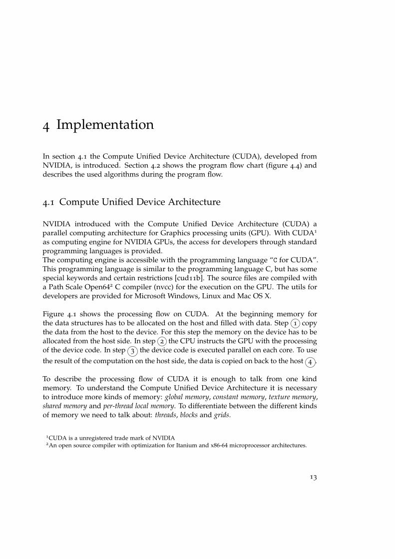
In section 4.1 the Compute Unified Device Architecture (CUDA), developed fromNVIDIA, is introduced. Section 4.2 shows the program flow chart (figure 4.4) anddescribes the used algorithms during the program flow.

4.1 Compute Unified Device Architecture

NVIDIA introduced with the Compute Unified Device Architecture (CUDA) aparallel computing architecture for Graphics processing units (GPU). With CUDA1

as computing engine for NVIDIA GPUs, the access for developers through standardprogramming languages is provided.The computing engine is accessible with the programming language “C for CUDA”.This programming language is similar to the programming language C, but has somespecial keywords and certain restrictions [cud11b]. The source files are compiled witha Path Scale Open642 C compiler (nvcc) for the execution on the GPU. The utils fordevelopers are provided for Microsoft Windows, Linux and Mac OS X.

Figure 4.1 shows the processing flow on CUDA. At the beginning memory forthe data structures has to be allocated on the host and filled with data. Step 1 copythe data from the host to the device. For this step the memory on the device has to beallocated from the host side. In step 2 the CPU instructs the GPU with the processingof the device code. In step 3 the device code is executed parallel on each core. To usethe result of the computation on the host side, the data is copied on back to the host 4 .

To describe the processing flow of CUDA it is enough to talk from one kindmemory. To understand the Compute Unified Device Architecture it is necessaryto introduce more kinds of memory: global memory, constant memory, texture memory,shared memory and per-thread local memory. To differentiate between the different kindsof memory we need to talk about: threads, blocks and grids.

1CUDA is a unregistered trade mark of NVIDIA2An open source compiler with optimization for Itanium and x86-64 microprocessor architectures.

13

4 Implementation

Host Memory

Device Memory

CPU

GPU

3

1 4 2

Figure 4.1: Processing flow on CUDA

The figure 4.2 shows the layers of CUDA. The atomic unit in CUDA is a single thread.Each thread has its own per-thread local memory. Not visualized in this figure are theregisters of the threads. In the next layer blocks of threads are defined by the developer.

Thread

Per−thread local memory

Shared memory

Block

Grid

Global memory

Block (0,0) Block (1,0)

Figure 4.2: Layers of CUDA

Therefore the attribute blockSize as an extension of the “C for CUDA” programminglanguage exists. All threads in a block are executed together with the Single InstructionMultiple Threads (SIMT) architecture. The blocks are distributed to different scalarprocessors within the same multiprocessor (MP). All threads in one block have access tothe same shared memory.In the last layer several blocks are combined as a grid. To define the amount of blocks

14

4.1 Compute Unified Device Architecture

in all grids the attribute gridSize exists. One grid of blocks is executed independently inserial or parallel and is distributed to different multiprocessors. All grids share thesame global memory.

The attributes blockSize and gridSize are organized in one, two or three dimen-sions. The blockSize and gridSize are defined before the execution of the kernel andso the blockSize and gridSize are the same for each multiprocessor in this execution.The size of each kind of memory is limited by the specification of the NVIDIA device.To get the values the NVIDIA CUDA LIBRARY provides the struct cudaDeviceProp.All significant attributes are listed in the CUDA API REFERENCE MANUAL [cud11a].

Lastly there are constant memory and texture memory, which not exist as physi-cal memory on the device. These kinds of memory reside in the global memoryand their maximal size is restricted by the device attributes. The constant memoryis read-only and not dynamically allocable. This kind of memory can be accesseddirectly from the device. From the host side it has to be copied as an symbol andis only indirectly accessible. The texture memory is also read-only, but it is possibleto bind data from the host to a texture. Applications for this kind of memory isheavily read-only data with irregular access patterns. A disadvantage of the texturememory is that no double precision support is provided. NVIDIA devices with supportof CUDA ≥ 3.1 provide additional surface memory, which allows read and write access.

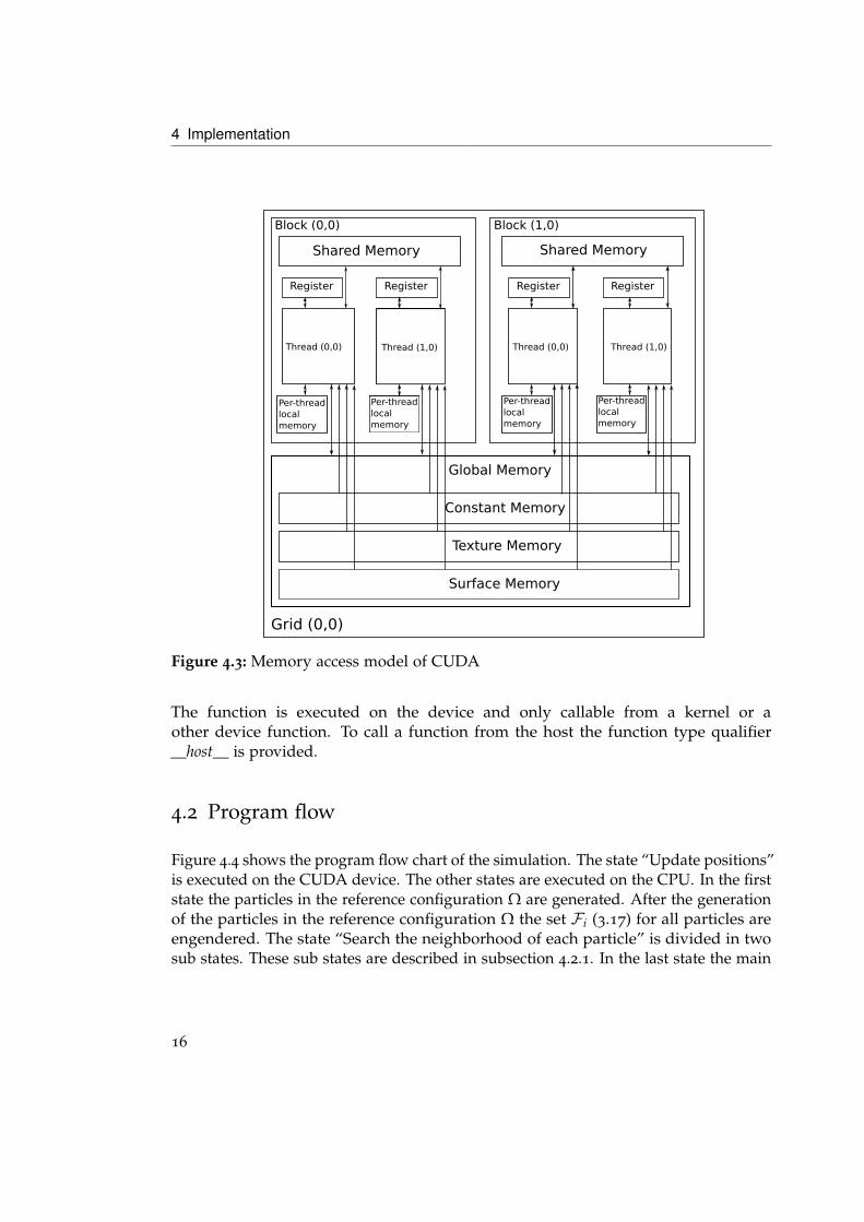
The figure 4.3 shows an overview of the different layers: threads, blocks and grids andthe different kinds of memory: global memory, constant memory, texture memory, sharedmemory and per-thread local memory, which are accessible from the different layers.

An important extension of the “C for CUDA” programming language are thefunction type qualifiers. The function type qualifiers specify where the function isexecuted and where the function is callable. For the execution on the device thequalifiers __global__ and __device__ exist.

A kernel is the entry point to start an execution on the CUDA device. A ker-nel is the only possibility to start an execution on the device and it is callable onlyfrom the host. A CUDA kernel has to be declared with the function type qualifier__global__. A restriction for the return type is, that a kernel allows no return typeand must have a void return type. A kernel call is asynchronous and returnsbefore the device has completed the execution.

To provide functions with a non void return type on the device, the functiontype qualifier __device__ is provided.

15

4 Implementation

Texture Memory

Constant Memory

Global Memory

Grid (0,0)

Register Register

Shared Memory

Thread (0,0) Thread (1,0)

Per-threadlocal memory

Per-thread localmemory

Shared Memory

Register Register

Thread (0,0) Thread (1,0)

Per-threadlocalmemory

Per-threadlocalmemory

Block (0,0) Block (1,0)

Surface Memory

Figure 4.3: Memory access model of CUDA

The function is executed on the device and only callable from a kernel or aother device function. To call a function from the host the function type qualifier__host__ is provided.

4.2 Program flow

Figure 4.4 shows the program flow chart of the simulation. The state “Update positions”is executed on the CUDA device. The other states are executed on the CPU. In the firststate the particles in the reference configuration Ω are generated. After the generationof the particles in the reference configuration Ω the set Fi (3.17) for all particles areengendered. The state “Search the neighborhood of each particle” is divided in twosub states. These sub states are described in subsection 4.2.1. In the last state the main

16

4.2 Program flow

Generate particles

Sort particles with the morton order

Find neighbors

Update positions

t < t_max

Search neighborhood of each particle

Figure 4.4: Program flow chart of the simulation. The green state of the diagram isexecuted on the CUDA device.

part of the Peridynamic is implemented. These states are executed on the NVIDIAdevice in parallel with CUDA. To boost up the computation time, the other states ofthe simulation should be ported to CUDA, but this is not part of this thesis.

4.2.1 Neighborhood search

For the discrete Peridynamic equation of motion the set Fi (3.17) has to be computedfor all particles. The naïve algorithm constructs the sets Fi in O(n2). A simpleoptimization for a equidistant lattice is to stop if the next length to the next particle is≥ δ. In this special case the algorithm is in O(n).To use a non equidistant lattice for the reference configuration Ω of the particlesanother algorithm is needed. In [Mic09] Connor and Kumar introduced an algo-rithm for the “construction of k-Nearest Neighbor Graphs for Point Clouds” inO(d n

pe · k · log(k)). The advantage of this algorithm is that randomly generated point

17

4 Implementation

clouds are supported. This means there is no restriction of the order of the particles inthe reference configuration Ω.

The algorithm [Mic09] uses the merge sort [Knu73] in combination with themorton order [TH81] to prepare the point cloud for an efficient search of the neighbors.The morton order or z order is a method to map multilevel data to one dimension.This method originally invented for databases and the approach is the concatenationof keys to generate a one dimensional code.

Figure 4.5: This figure illustrates the space filling curve for the morton order / z orderin the upper part. The lower part shows an example for the z values for0 ≤ x, y ≤ 3.

The figure 4.5 illustrates the space filling curve for the z order in the upper part. In theupper part the one dimensional code (z values) for the two dimensional point cloud0 ≤ x, y ≤ 3 is computed. The curve between the z values is named z curve.The library STANN [STA] is the C++ implementation of the algorithm “Fast construc-tion of k-Nearest Neighbor Graphs for Point Clouds” described in [Mic09]. Thislibrary is used for the neighbor search in the simulation. To verify the scaling of therun time of the STANN library the run time with a equidistant lattice was measuredand plotted in figure 4.6.

4.2.2 Update Positions

The last state of the program flow chart (4.4) is implemented with the “C for CUDA”programming language. In the first part of this section the CUDA kernel is described.

18

4.2 Program flow

0

50

100

150

200

250

300

350

400

450

0 1e+06 2e+06 3e+06 4e+06

Com

puta

tion

time

(sec

onds

)

#Particle

STANN Library (0.74) [Intel i7-2600 @ 3.4GHz (1 Core), 15.6 GiB, Scientific Linux 6.1, Kernel 2.6.32, gcc 4.4.5]

Figure 4.6: Run time of the STANN library on a equidistant two dimensional lattice.

The part of the code of the “C for CUDA” programming language, which is executedon the CUDA device, is called a CUDA kernel.The second part of this section contains the restrictions for the theoretical maximalamount of particles. The theoretical maximal amount of particles depends on thespecification of the CUDA device. An equation (4.2) for the theoretical maximalamount and some examples for the NVIDIA GeForce GTX 560 Ti, the used CUDAdevice in this thesis, are provided.

4.2.2.1 Parallelization of the discrete Peridynamic equation of motion

The implementation of the discrete Peridynamic equation of motion (3.18) with the “Cfor CUDA” programming language is shown in the listing 4.1. The kernel containsfour steps, but the last one is optional for improved visualization of the simulationresults.The step 0 initialize the vectors for the inner force fi in the first time step. In all othertime steps the vectors have to need to be reset, because the inner force fi is not historydependent. In 1 the discrete Peridynamic equation of motion (3.18) is computedfor each particle. So the information about the acceleration yt

i on each particle Pi attime t is there. To compute the position of each particle Pi at time t the Störmer–Verletmethod (3.22) is used in 2 .

19

4 Implementation

The step 3 contains not really to the Peridynamic, but is needed to produce thefigures in section 6.2. To measure the computation time of the CUDA kernel thecomputation time with step 3 and without step 3 is behold.

4.2.2.2 Maximal amount of particles

The figure 4.7 shows the data structures on the CUDA device. The lower data structurehas the size of n · k, with n as the amount of particles and k as the maximal amountof neighbors.

xActxInit

xBefore

neighbours N

#neighbor

fi

R3

R3

R3

R3

R

Figure 4.7: This figure shows the data structures on the CUDA device. The upper datastructures are linear in the size of n. The lower data structure has the sizeof n · k, with n as the amount of particles and k as the maximal amount ofneighbors.

The equation 4.1 shows the usage of memory on the CUDA device. The number n isthe amount of particles and k the maximal number of neighbors per particle.

[4 · 3 · sizeo f (double) + sizeo f (int) + (k + 1) · sizeo f (int)] · n (4.1)

The size of the global memory on a device restricts the maximal number of particlesper computation. In C++ and in “C for CUDA” the size of a double is 8 bytes and thesize of an integer is 4 Bytes. We assume that N is the size of the global memory onour CUDA device. Equation 4.2 defines the maximal amount of particle on the CUDAdevice.

n =

⌊N

4 · 3 · 8 + 4 + (k + 1) · 4

⌋=

⌊N

104 + 4 · k

⌋(4.2)

The NVIDIA GeForce GTX 560 Ti, the used CUDA device in this thesis, provides2.146.631.680 bytes as global memory.

20

4.2 Program flow

Listing 4.1 The parallel computation of the equation of motion and the estimation ofthe new positions on the CUDA device

1 __global__ UpdatePositions( ... )

for all time steps4

// 0 Initialize the inner forces7

for all particles

10 fi index = 0, 0, 0;__syncthreads();

13

// 1 Compute the acceleration for each particlefor all particles

16

yni =

∑j∈Fi

f (unj −un

i ,xj−xi)VjVi

p(xi)Vi

19 __syncthreads();

// 2 Compute the new position of each particle22 for all particles

xn+1

i = 2 · xni − xn−1

i + yni · 4t2

25 __syncthreads();

28 // 3 Compute the updated amount of neighbors for each particlefor all particles

31 for all neighbors

//Update the amount of neighbors for each particle34

37 __syncthreads();

21

4 Implementation

4.3 Measurement of the computation time

There exist several implementations of the Peridynamic technique [Sana, PSP+11,

SIE11], but none of them has no native support of CUDA. All of them are implementedin FORTRAN or C++ and executed on single core CPU or multi core CPU’s.Another possibility is to use a GPU to implement the Peridynamic technique. Animportant attribute for a simulation is the computation time, especially for large entities.So the computation time for following two implementations of the Peridynamictechnique are compared:

1. CUDA (NVIDIA GeForce GTX 560 Ti)

• Host: Scientific Linux (6.1) with Kernel 2.6.32.1

• gcc 4.4.5 (-O3 -m64)

• nvcc 4.0 V.2.1221 (-m64 -arch=sm_21 -use_fast_math)

2. Single core (Intel i7-2600 @ 3.4GHz)

• Host: Scientific Linux (6.1) with Kernel 2.6.32.1 and 16 GiB RAM

• gcc 4.4.5 −O3

To compare different implementations or algorithms a measurement for the compara-tive property is needed:

“A software metric is any measurement which relates to a software system,process or related documentation.” [Iva89]

The software engineering provides software metrics for objective, reproducible andquantifiable measurements . Software metrics are classified in two classes: controlmetrics and predictor metrics. Predictor metrics are measurements to compare thequality of to software products. To compare the two implementations the followingmetric (4.3) is defined:

m1 =computation time

#particles(4.3)

Figure 4.8 shows the computation time of the Peridynamic technique for on particleper time step. The first aspect is that the computation time on the GPU is articulatelyfaster per particle and the difference is medial 3.0.This value is feasible, because the processing power for NVIDIA GeForce GTX 560 Ti[Har] in double precision is 105 GFLOPS and the processing power for the Intel i7-2600@ 3.4GHz [Mar] is 83 GFLOPS. For a single thread the processing power for the Intel

22

4.4 Challenges with the Compute Unified Device Architecture

i7-2600 @ 3.4GHz sinks to ≈ 21 GFLOPS. The theoretical value for the difference in thecomputation time between the GPU and CPU is 105 GFLOPS

21 GFLOPS = 5.

0

0.005

0.01

0.015

0.02

0.025

0.03

0.035

0.04

0.045

0.05

0 500000 1e+06 1.5e+06 2e+06 2.5e+06 3e+06

Com

puta

tion

time

/ #Pa

rticl

e (m

s)

#Particle

NVIDIA GeForce GTX 560 Ti [1] vs. Intel i7-2600 @ 3.4GHz (1 Core) [2]

GPU [1]i7 core [2]

Figure 4.8: Run time of the different implementations for one particle per time step.

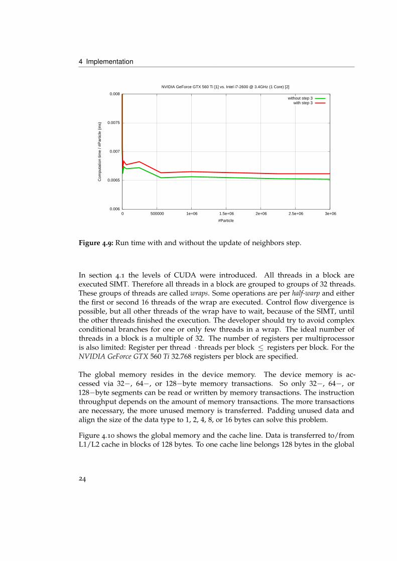
Figure 4.9 shows the run time of the CUDA kernel (4.1) with step 3 and without 3 .The step 3 is not part of the Peridynamic, but delivers additional information for thevisualization.

4.4 Challenges with the Compute Unified Device Architecture

This section contains a summary of challenges with the Compute Unified DeviceArchitecture. The test [Har] of the processing power for NVIDIA GeForce GTX 560Ti results 1.263 GFLOPS for single precision. In the Peridynamic theory small timesteps in the range of 10−9 − 10−6 are the standard for most simulations. This causessmall changes in the values during the simulation and it is necessary to use doublerecession. For double precision the processing power NVIDIA GeForce GTX 560 Tisinks to 105 GFLOPS. Compared to the test [Mar] of the CPU Intel Core i7 2600K 3.40GHz with 83 GFLOPS the benefit of the GPU shrinks.

23

4 Implementation

0.006

0.0065

0.007

0.0075

0.008

0 500000 1e+06 1.5e+06 2e+06 2.5e+06 3e+06

Com

puta

tion

time

/ #Pa

rticl

e (m

s)

#Particle

NVIDIA GeForce GTX 560 Ti [1] vs. Intel i7-2600 @ 3.4GHz (1 Core) [2]

without step 3with step 3

Figure 4.9: Run time with and without the update of neighbors step.

In section 4.1 the levels of CUDA were introduced. All threads in a block areexecuted SIMT. Therefore all threads in a block are grouped to groups of 32 threads.These groups of threads are called wraps. Some operations are per half-warp and eitherthe first or second 16 threads of the wrap are executed. Control flow divergence ispossible, but all other threads of the wrap have to wait, because of the SIMT, untilthe other threads finished the execution. The developer should try to avoid complexconditional branches for one or only few threads in a wrap. The ideal number ofthreads in a block is a multiple of 32. The number of registers per multiprocessoris also limited: Register per thread · threads per block ≤ registers per block. For theNVIDIA GeForce GTX 560 Ti 32.768 registers per block are specified.

The global memory resides in the device memory. The device memory is ac-cessed via 32−, 64−, or 128−byte memory transactions. So only 32−, 64−, or128−byte segments can be read or written by memory transactions. The instructionthroughput depends on the amount of memory transactions. The more transactionsare necessary, the more unused memory is transferred. Padding unused data andalign the size of the data type to 1, 2, 4, 8, or 16 bytes can solve this problem.

Figure 4.10 shows the global memory and the cache line. Data is transferred to/fromL1/L2 cache in blocks of 128 bytes. To one cache line belongs 128 bytes in the global

24

4.4 Challenges with the Compute Unified Device Architecture

Figure 4.10: Global memory and caching

memory. To improve the performance the access to the global memory should becoalesced. If multiple threads of a wrap access the same cache line the accesses arecombined into one memory transfer.

The last advice for improvement of performance is to use fast mathematicaloperations, e. g __sprt(. . . ), if it is possible. These functions are less accurate, butexecuted faster. The compile flags -use_fast_math has been set to get correct results ofthe fast mathematical operations.

25

5 Combination with the Partition of UnityMethod

The Partition of Unity Method (PUM) is introduced in [MB96, pum97]. In [Sch03] theabstract ingredients are:

• A Partition of the unity ϕi | i = 1, . . . , N with ϕi ∈ Cr(RD, R) and patchesωi := supp(ϕi),

• a collection of local approximation spaces

Vi(ωi, R) := span〈ϑni 〉 (5.1)

defined on the patches ωi , i = 1, . . . , N.

The combination of these two ingredients is the following:

VPU :=N

∑i=1

ϕiVi = span〈ϕiϑni 〉 (5.2)

A property of the PUM is that the approximation spaces Vi can be chosen independentof each other. So it is possible to combine the Peridynamic theory with a FiniteElement Method (FEM), e. g. PUM. The figure 5.1 shows an approach to combinethese two methods. The body R in the reference configuration Ω is divided in twoareas ΩPUM and ΩPeridynamic. The area ΩPeridynamic in the reference configuration Ωis placed at the position with an initial crack or at the place where a fracture ispresumably. In the figure 5.1 there is a initial crack with the color magenta. Theremaining area in the reference configuration Ω is simulated with the PUM.First several time steps with the PUM are simulated and then the boundary forcefbound is exchanged over the boundary of the two areas ΩPUM and ΩPeridynamic. Theexchange of the boundary force fbound is done with the discrete Peridynamic equationof motion (3.18, 3.21). The discrete Peridynamic equation of motion has the additiveterm b(xi, t) on the right side. This term is used to model extern forces on particle atposition x at time t.

Secondly several time steps of the Peridynamic are simulated. After the simu-lation the displacement field u = Xi | i = 1, . . . , N with Xi as the position of all

27

5 Combination with the Partition of Unity Method

Boundary Forces Enrichment Functions

ΩPeridynamic

ΩPUM

Figure 5.1: Combination with the Partition of Unity Method

particles at time step i exists. With the displacement field u it is possible to generateenrichment functions, which can be used to simulate the next time steps of the PUM.

The generation of the enrichment functions is not part of this thesis. More in-formation about their generation of the enrichment functions can be found in thespecial research field 716, sub project D.7 [Col12].

28

6 Results

In this Chapter are two different possibilities to use the Peridynamic model on solidmechanics. In the first experiment an thick square plate with an initial crack wereused for the geometry. In this scenario the growing of the crack is interesting. Thesecond experiment simulates the impact of an projectile into an cylinder. In this casethe interest is in the appearance of cracks.

6.1 Experiment 1

This experiment was inspired from the publication “A mesh-free method based on thePeridynamic model of solid mechanics” [SA05]. The experiment in the publicationuses velocity boundary conditions. Velocity boundary conditions are not available inthe Peridynamic technique introduced in [Sil00]. In [Sil98] in section 13 and section 14a formulation of the Peridynamic technique with boundary conditions is presented.The figure 6.1 shows the geometry of the thick square plate. In the center of the slimsquare plate in an horizontal initial crack with the length of 10 mm.

In this experiment the thick square plate receives an first pulse, which generates tensilestress waves. This waves move towards the crack and start the growing of the crack.The second pulse is an compressive pulse and stops the growing of the crack. Thefigure 6.2 shows the forces on the thick square plate. The forces are applied on eachhalf of the thick square plate.

The table 6.1 contains the simulation parameters for this experiment.

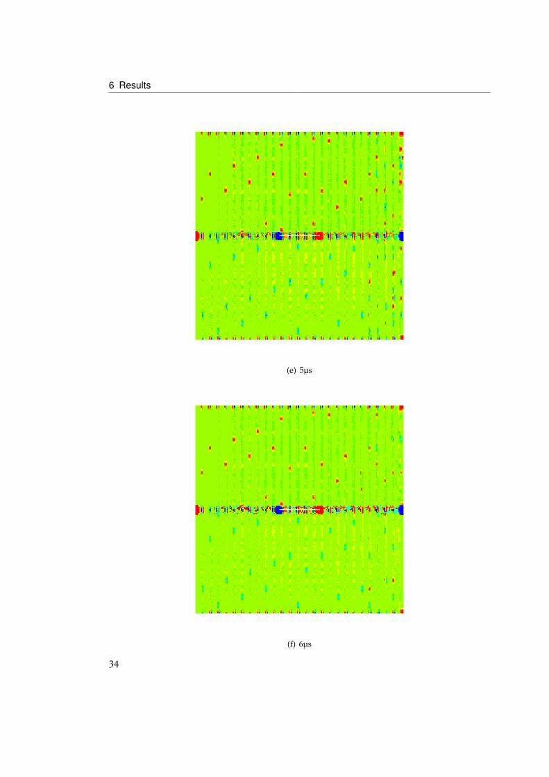
Figure 6.3 shows the growing of the crack and the waves moving to the crack in thefirst 5 time steps. Figure 6.3 shows the compressive pulse and the delay of the crack inthe last 5 time steps. This experiment is not the same as in the publication, becausevelocity boundary conditions are not available in the Peridynamic technique used inthis thesis. This result shows that it is possible to simulate growing and delay of crackswith the Peridynamic technique described in [Sil00].

29

6 Results

(a) Blueprint of the thick square plate. (b) Reference configuration Ω of the body R.Particles are colored by the amount of neighbors.

Figure 6.1: Blueprint and reference configuration Ω of the body R (experiment 1).

freefree

5 10

-20 00t(ns)

b(t)b(t)

−b(t)

20 00

Figure 6.2: Forces on the horizontal edges on the thick square plate.

30

6.1 Experiment 1

Parameter Value

Density $ 8000kgm2

Young’s modulus k 192 PaLength of horizon δ 1.6 mmCritical stretch for bound failure s00 0.02∆x 0.25 mm∆y 0.25 mm∆z 0.25 mm#Particles 39920time step 1µsstep size 10

Table 6.1: Simulation parameters for experiment 1

31

6 Results

(a) 1µs

(b) 2µs

32

6.1 Experiment 1

(c) 3µs

(d) 4µs

33

6 Results

(e) 5µs

(f) 6µs

34

6.1 Experiment 1

(g) 7µs

(h) 8µs

35

6 Results

(i) 9µs

(j) 10µs

Figure 6.3: Growing of the crack (1µs–5µs) and delay of the crack (6µs–10µs).Particles are colored by the acceleration in x–direction.

36

6.2 Experiment 2

6.2 Experiment 2

The Experiment 2 was adapted from the publication “Implementing Peridynamicwithin a molecular dynamics code” [P+

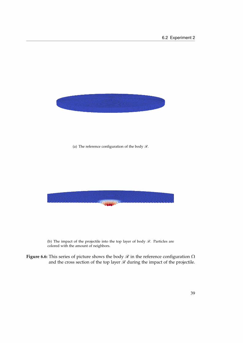
08]. The figure 6.4 shows the geometry of thecylinder. In this experiment the impact of an projectile was simulated. The projectile ismodeled as an rigid sphere with the diameter 0.01m and an indenter, exerting forceF(r) = −1 · 1017(r− R)2. The scenario of the impact is shown in figure 6.5.

Figure 6.4: Blueprint of the cylinder.

0.0205m

r=0.005m

v = 100ms

F(r) = −1 · 1017(r− R)2

Figure 6.5: Model, measurements and forces of the projectile.

37

6 Results

Parameter Value

Density $ 2200kgm2

Young’s modulus k 14.9 GPaLength of horizon δ 0.0005 mCritical stretch for bound failure s00 0.0005∆x 0.0005 m∆y 0.0005 m∆z 0.0005 m#Particles 83250time step 1nsstep size 100000

Table 6.2: Simulation parameters for experiment 2

38

6.2 Experiment 2

(a) The reference configuration of the body R.

(b) The impact of the projectile into the top layer of body R. Particles arecolored with the amount of neighbors.

Figure 6.6: This series of picture shows the body R in the reference configuration Ωand the cross section of the top layer R during the impact of the projectile.

39

6 Results

(a) 10ns

(b) 50ns40

6.2 Experiment 2

(c) 150ns

(d) 225ns 41

6 Results

(e) 275ns

(f) 30ns42

6.2 Experiment 2

(g) 375ns

(h) 400ns

Figure 6.7: Top layer of the body R during the impact. Particles are colored by theamount of neighbors.

43

7 Conclusion and outlook

This thesis proves that it is possible to use the Compute Unified Device Architecturefor the implementation of a Peridynamic technique on a GPU. In chapter 6 the resultsof the two experiments described in [SA05, P+

08] are showing that it was possibleto reproduce the two numerical experiments on the GPU with similar results. Thisproves that the Peridynamic technique was correctly implemented on the GPU withCUDA and it is possible to use the fast mathematical operations which are executedfaster, but which are therefore less accurate.

In chapter 4.3 the implementation on the GPU is compared with the CPU im-plementation. To compare the two implementations a software metrics for objective,reproducible and quantifiable measurements has been defined. The results ofthe comparison with the metric presented in chapter 4.3 are plotted in figure 4.8.Considering metric presented in chapter 4.3 the GPU implementation is a factor ≈ 3faster in the computation time for one step of the Peridynamic technique for oneparticle. Consider the theoretical factor by comparing the double precision floatingpoint performance (PEAK) of the two devices is ≈ 5.0. In this case the measureddifference in the computation time for one step of the Peridynamic technique for oneparticle is appropriate.

Outlook

Following improvements of the software are recommended:

1. Running the software on a High Performance Computing GPU.

2. Porting the other states to CUDA.

3. Boundary conditions as described in [Sil98].

The first improvement for the computation time is to use a High PerformanceComputing (HPC) GPU for the simulation. NVIDIA provides GPUs for differentapplication areas and the NVIDIA GeForce GTX 560 Ti is designed for the gamingapplication area. For the application area HPC the NVIDIA Tesla 20 Serie is provided.

45

7 Conclusion and outlook

The advantage of NVIDIA Tesla 20 Serie for simulations is the accession of processingpower in double precision. For example, the double precision floating point perfor-mance (PEAK) for the NVIDIA TESLA1 C2075 is specified with 515 GFLOP’s [NVI12].The double precision floating point performance (PEAK) for the NVIDIA GeForce GTX560 Ti is measured with 105 GFLOP’s [Har]. It is theoretically possible to reduce thecomputation time by a factor 5 by using the NVIDIA TESLA C2075. The source codein the “C for CUDA” programming language can be compiled for different devicearchitectures, but in most cases some customizing because of other device features hasto be done.

The second improvement is to port the other states of the program flow chart(figure 4.4) to CUDA. The first state “Generate particles” can be easily ported toCUDA because the initial position of the particles in the reference configuration Ω hasto be generated. In order to port the state “Search neighborhood of each particle” toCUDA, a parallel sorting algorithm with the morton order has to be implemented inCUDA first. In [SHG09] efficient sorting algorithms for many core GPUs are presented.Secondly the neighbor search has to be implemented into CUDA. In [GSSP10] analternative algorithm for the neighbor search in CUDA is presented.

The third improvement is the implementation of the boundary conditions asdescribed in [Sil98]. Boundary conditions are important in the conventional theory ofcontinuum mechanics for specific solutions in equilibrium problems.

1TESLA is a unregistered trade mark of NVIDIA

46

Bibliography

[Col12] Collaborative Research Center (SFB) 716. Meshfree Multiscale Methodsfor Solids, 2012. URL http://www.sfb716.uni-stuttgart.de/forschung/teilprojekte/projektbereich-d/d7.html. (Quoted on page 28)

[cud11a] CUDA API REFERENCE MANUAL. 4.0. NVIDIA, 2011. (Quoted on page 15)

[cud11b] NVIDIA CUDA C Programming Guide. 4.0. NVIDIA, 2011. (Quoted onpage 13)

[Edw02] H. C. Edwards. SIERRA Framework Version 3: Core Services Theory andDesign. Technical report, Sandia National Laboratories, 2002. (Quoted onpage 3)

[ELP] E. Emmrich, R. B. Lehoucq, D. Puhst. "Peridynamics: a nonlocal continuumtheory". (Quoted on page 5)

[GSSP10] P. Goswami, P. Schlegel, B. Solenthaler, R. Pajarola. Interactive SPH Sim-ulation and Rendering on the GPU. In M. Otaduy, Z. Popovic, editors,Eurographics/ ACM SIGGRAPH Symposium on Computer Animation. 2010.(Quoted on page 46)

[Har] HardTecs4U. NVIDIA GeForce GTX 560 TI im Test. URLhttp://ht4u.net/reviews/2011/nvidia_geforce_gtx_560_ti_msi_n560ti_twin_frozr_2/index2.php. (Quoted on the sides 22, 23 and 46)

[HLW03] E. Hairer, C. Lubich, G. Wanner. Geometric numerical integration illustratedby the Störmer/Verlet method. Acta Numerica, 12:399–450, 2003. (Quoted onpage 12)

[Iva89] Ivan Summerville. Software Engineering. 3. Addision Wesley, 1989. (Quotedon page 22)

[Knu73] D. E. Knuth. THE ART OF COMPUTER PROGRAMMING, volume 3. Addi-sion Wesley, Stanford University, 1973. (Quoted on page 18)

[Mar] Marc Büchel. Sandy Bridge: Core i7 2600K und Core i5 2500K.URL http://www.ocaholic.ch/xoops/html/modules/smartsection/item.php?itemid=452&page=6. (Quoted on the sides 22 and 23)

vii

Bibliography

[MB96] J. Melenk, I. Babuška. The Partition of Unity Finite Element Method: Ba-sictheory and applications. Computer Methods in Applied Mechanics andEngineering, 139:289–314, 1996. (Quoted on page 27)

[Mic09] Michael Connor and Piyush Kumar. Fast construction of k-Nearest NeighborGraphs for Point Clouds. In IEEE TRANSACTIONS ON VISUALIZATIONAND COMPUTER GRAPHICS. 2009. (Quoted on the sides 17 and 18)

[NVI12] NVIDIA. NVIDIA TESLA C2075 COMPANION PROCESSOR CALCULATERESULTS EXPONENTIALLY FASTER, 2012. URL http://www.nvidia.com/docs/IO/43395/NV-DS-Tesla-C2075.pdf. (Quoted on page 46)

[P+08] M. L. Parks, et al. Implementing peridynamics within a molecular dynam-

ics code. In Computer Physics Communications, volume 179, pp. 777–783.ELSEVIER, 2008. (Quoted on the sides 9, 10, 37 and 45)

[Pli95] S. Plimpton. Fast Parallel Algorithms for Short–Range Molecular Dynamics.In Journal of Computational Physics, volume 117, pp. 1 – 19. 1995. (Quoted onpage 3)

[PSP+11] M. L. Parks, P. Seleson, S. J. Plimpton, S. A. Silling, R. B. Lehoucq. Peridy-

namics with LAMMPS: A User Guide v0.3 Beta. SANDIA REPORT, SandiaNational Laboratories, 2011. (Quoted on the sides 3 and 22)

[pum97] The Partion of Unity Method. International Journal for Numerical Methods inEngineering, 40:727–758, 1997. (Quoted on page 27)

[SA05] S. A. Silling, E. Askari. A meshfree method based on the peridynamic modelof solid mechanics. In Computer & Structures, volume 83, pp. 1526–1535.ELSEVIER, 2005. (Quoted on the sides 29 and 45)

[Sana] Sandia National Laboratories. EMU. URL http://www.sandia.gov/emu/emu.htm. (Quoted on the sides 3 and 22)

[Sanb] Sandia National Laboratories. LAMMPS Molecular Dynamics Simulator.URL http://lammps.sandia.gov/. (Quoted on page 3)

[Sch03] M. A. Schweitzer. Parallel Multilevel Partition of Unity Method for EllipticPartial Differential Equations, volume 29. Springer, 2003. (Quoted on page 27)

[SHG09] N. Satish, M. Harris, M. Garland. Designing Efficient Sorting Algorithms forManycore GPUs, 2009. To Appear in Proc. 23rd IEEE International Paralleland Distributed Processing Symposium. (Quoted on page 46)

viii

Bibliography

[SIE11] SIERRA Solid Mechanics Team. Sierra/SolidMechanics 4.22 User’s Guide.Technical report, Computational Solid Mechanics and Structural DynamicsDepartment (Sandia National Laboratories), 2011. (Quoted on the sides 3

and 22)

[Sil98] S. A. Silling. Reformulation of elasticity theory for discontinuities and long-range forces. Technical report, Sandia National Laboratories, 1998. (Quotedon the sides 29, 45 and 46)

[Sil00] S. A. Silling. Reformulation of elasticity theory for discontinuities and long-range forces. In Journal of the Mechanics and Physics of Solids, volume 48, pp.175–209. Pergamon, 2000. (Quoted on the sides 5 and 29)

[STA] STANN. URL https://sites.google.com/a/compgeom.com/stann/Home.(Quoted on page 18)

[TH81] H. Tropf, H. Herzog. Multidimensional Range Search in DynamicallyBalanced Trees. In Angewandte Informatik (Applied Informatics), pp. 71–77.Vieweg Verlag, 1981. (Quoted on page 18)

All links were last followed on March 12, 2012.

ix

Declaration

All the work contained within this thesis,except where otherwise acknowledged, wassolely the effort of the author. At nostage was any collaboration entered intowith any other party.

(Patrick Diehl)