Implementation of Dynamic Matrix Control for Non-Linear system · 2016-04-23 · Implementation of Dynamic Matrix Control for Non-Linear system Ramesh.S1, ... coefficient for the

International Research Journal of Engineering and Technology (IRJET) e-ISSN: 2395 -0056

Volume: 03 Issue: 03 | Mar-2016 www.irjet.net p-ISSN: 2395-0072

© 2016, IRJET | Impact Factor value: 4.45 | ISO 9001:2008 Certified Journal | Page 1397

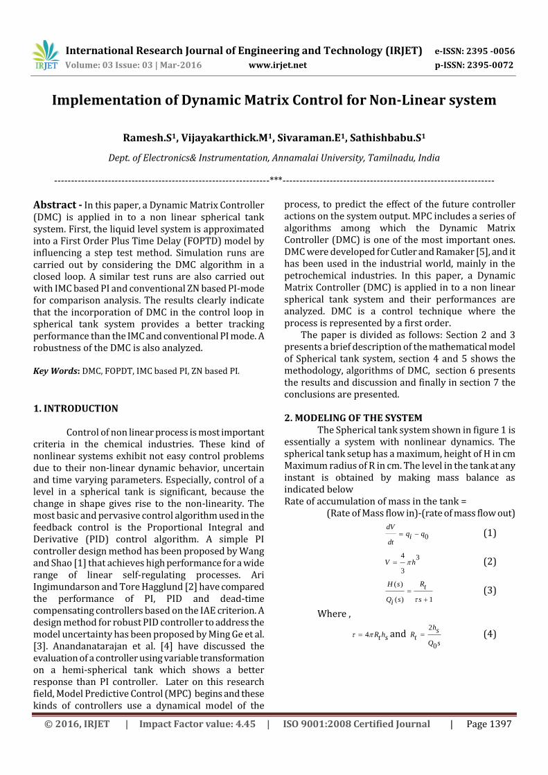
Implementation of Dynamic Matrix Control for Non-Linear system

Ramesh.S1, Vijayakarthick.M1, Sivaraman.E1, Sathishbabu.S1

Dept. of Electronics& Instrumentation, Annamalai University, Tamilnadu, India

----------------------------------------------------------------***---------------------------------------------------------------

Abstract - In this paper, a Dynamic Matrix Controller (DMC) is applied in to a non linear spherical tank system. First, the liquid level system is approximated into a First Order Plus Time Delay (FOPTD) model by influencing a step test method. Simulation runs are carried out by considering the DMC algorithm in a closed loop. A similar test runs are also carried out with IMC based PI and conventional ZN based PI-mode for comparison analysis. The results clearly indicate that the incorporation of DMC in the control loop in spherical tank system provides a better tracking performance than the IMC and conventional PI mode. A robustness of the DMC is also analyzed.

Key Words: DMC, FOPDT, IMC based PI, ZN based PI.

1. INTRODUCTION

Control of non linear process is most important criteria in the chemical industries. These kind of nonlinear systems exhibit not easy control problems due to their non-linear dynamic behavior, uncertain and time varying parameters. Especially, control of a level in a spherical tank is significant, because the change in shape gives rise to the non-linearity. The most basic and pervasive control algorithm used in the feedback control is the Proportional Integral and Derivative (PID) control algorithm. A simple PI controller design method has been proposed by Wang and Shao [1] that achieves high performance for a wide range of linear self-regulating processes. Ari Ingimundarson and Tore Hagglund [2] have compared the performance of PI, PID and dead-time compensating controllers based on the IAE criterion. A design method for robust PID controller to address the model uncertainty has been proposed by Ming Ge et al. [3]. Anandanatarajan et al. [4] have discussed the evaluation of a controller using variable transformation on a hemi-spherical tank which shows a better response than PI controller. Later on this research field, Model Predictive Control (MPC) begins and these kinds of controllers use a dynamical model of the

process, to predict the effect of the future controller actions on the system output. MPC includes a series of algorithms among which the Dynamic Matrix Controller (DMC) is one of the most important ones. DMC were developed for Cutler and Ramaker [5], and it has been used in the industrial world, mainly in the petrochemical industries. In this paper, a Dynamic Matrix Controller (DMC) is applied in to a non linear spherical tank system and their performances are analyzed. DMC is a control technique where the process is represented by a first order.

The paper is divided as follows: Section 2 and 3 presents a brief description of the mathematical model of Spherical tank system, section 4 and 5 shows the methodology, algorithms of DMC, section 6 presents the results and discussion and finally in section 7 the conclusions are presented.

2. MODELING OF THE SYSTEM

The Spherical tank system shown in figure 1 is essentially a system with nonlinear dynamics. The spherical tank setup has a maximum, height of H in cm Maximum radius of R in cm. The level in the tank at any instant is obtained by making mass balance as indicated below Rate of accumulation of mass in the tank = (Rate of Mass flow in)-(rate of mass flow out)

0

dVq qi

dt

(1)

4 3

3

V h (2)

( )

( ) 1

RH s t

Q s si

(3)

Where ,

4 R ht s and 2

0

hsRt

Q s

(4)




Fig – 1: Spherical Tank Liquids level

Let,

qI – Inlet flow rate to the tank (m3 /min)

qo – Outlet flow rate to the tank (m3 /min)

H – Height of the Spherical tank(m)

h- Height of the liquid level in the tank

at any time „t‟(m)

R- Top radius of the Spherical tank (m)

r – Radius of the conical Vessels

at a particular level of height h(m)

A – Area of the Spherical tank (m2)

3. BLACK BOX MODELING In real time implementation, initially the level in the tank is maintained at steady state of 10% (5 cm) of the total height. A step size of 5% in DAC output is given to the system. The variation in level (%) is recorded against time until a new steady state is attained Table .1. Transfer function model of Spherical tank at different operating points

Level Transfer Function

10%

1204.5( )

440 1

seG s

s

50%

1306( )

1200 1

seG s

s

66%

1502.75( )

1050 1

seG s

s

From the experimental data the FOPTD model parameters such as process gain (Kp), time delay (D) and time constant (τp,) of the level process are

determined. The same procedure is repeated at 50% and 66% of the total level and the identified transfer function models for all the above operating point is given in Table 1. 4. FINITE STEP RESPONSE MODEL

FSR models are obtained by making a unit step input change to a process operating at steady state. The model coefficients are simply the output values at each time step. Here,Si represents the step response coefficient for the ith sample time after the unit step change. If a non-unit step change is made, the output is scaled accordingly.

The step response model is the vector of step response coefficients, S = [ s1 s2 s3 s4 s5 . . . . . sN]T (5) Where N is the model length 5. DYNAMIC MATRIX CONTROL ALGORITHM

Dynamic matrix control based on step response model,

= + + . . . + +

(6) This is written in the form

= + (7)

Where, is the model prediction at time step k

is the manipulated input N steps in the past.

Note that the model – prediction output is unlikely to be equal to the actual measured output at time step k. Additive disturbance,

= - (8)

Where

is actual measured output

is the model prediction

The corrected prediction is then equal to the actual measured output at step k

= + (9)

Similarly, the corrected predicted output at the jth time step in future can be found from

= + (10)

= + + +

(11) Where, is the effect of future control

moves + is the effect of

past control moves is the correction term




The most common assumption is that the correction term is constant in future

= = . . .= = - (12)

Also, realize that there are no control moves beyond the control horizon of M steps, so

= =...= =0 (13)

In matrix – vector form, a prediction horizon of P steps and a control horizon of M steps yields

In matrix – vector form, a prediction horizon of P steps and a control horizon of M steps yields

ˆ1

0 0 0 01ˆ2 0 0 02 1

1

1 2 1ˆ2

11 2 1

ˆ

cyk

scuy kk s s

uk

c s s s sj j j j My uk j k M

uk Ms s s sP P P P Mc

yk P

2

103 420 0

0 01 23

20 0

3 4 2 1

5 1

1

1 2

s s s s s

uks s s suk

s s sj juk N

uk Ns s

N N

N

N

P P

1

2

1

2

3

uk N

uk NsN

uk N P

dk

dk

dk

dk P

(14)

Which we write using matrix notation ˆˆc

Y s u s u s u dpast past N Pf f

(15) In the above equation, the corrected predicted output response is naturally composed of a ‘forced response’ (contributions of the current and future control moves) and a ‘free response’ (the output changes that are predicted if there are no future control moves).the difference between the set point trajectory , r, and the future prediction is

ˆˆ [ ]c

past P N P f fr Y r s u s u d s u (16)

This can be written as c

f fE E s u (17)

Where

cE is the future predicted error E is the free response

-f fs u is the forced response

The least squares objective function is

22 1

1 0

P Mce w uk i k i

i i

(18)

Where

12

21 21

cekceP c c c c ke e e e

k i k k k Picek P

(19)

= Tc cE E (20)

And

21 1

1 10

1

uk

uM kw u w u u uk i k k k Mi

uk M

(21)

0 0 0

0 0 0 11 1 0 0 0

0 0 01

uw k

uw ku u uk k k M

w uk M

(22)

= Tu w uf f

(23)

Therefore the objective function can be written in the form

= TTc cE E u w u

f f (24)

By Substituting equation 17, the constrain into objective function can be

written T T

E s u E s u u w uf f f f f f

(25) The solution of the minimization of this objective function is

uf

1

T Ts s w sf f f

.E (26)

Notice that the current and future control moves

vector( uf

) is proportional to the unforced

error vector( E ) . that is controller gain matrix, K multiplies the unforced error vector.

fu =K E (27)

Where K = 1

T Ts s w sf f f

Because only the current control moves is actually implementing, we use the first row of the K matrix, and




fu =K1 E (28)

Where K1 represents the first row of the K matrix 5.1. Steps involved in Implementing DMC on a process

1. Develop a discrete step response model with length N, based on the sample time ∆t.

2. Specify the prediction (P) and control (M) horizons. That is N≥P≥M

3. Specify the weighting on the control action (w=0 if no weighting).

4. All calculations assume deviations variable form, so remember to covert to/from physical units.

5.2. DMC Tuning Strategy 1. Approximate the process dynamics with a first

Order plus dead time (FOPDT) model

( )

( ) 1

t sdK eY s p

U s sp

(29)

2. It is desirable but not necessary to select a value for the sampling interval, T. if possible, select T as the largest value that satisfies

0.1T p and 0.5T td

(30)

3. Calculate the discrete dead time (rounded to the next

integer): 1

tdkT

(31) 4. Calculate the prediction horizon and the model horizon as the process settling time in samples (rounded to the next integer):

5 pP N k

T

(32)

5. Select the control horizon, M (integer, usually from 1 to 6) and calculate the move suppression

coefficient:

0

3.5 12

500 2

p

f

MMf

T

1

1

M

M

(33) 2fK p (34)

6. Implement DMC using the traditional step response matrix of the actual process and the following parameters computed in steps 1-5:

Sample time, T Model horizon (process settling time in samples),

N

Prediction horizon (optimization horizon), P Control horizon (number of moves), M

Move suppression coefficient, 6. SIMULATION RESULTS

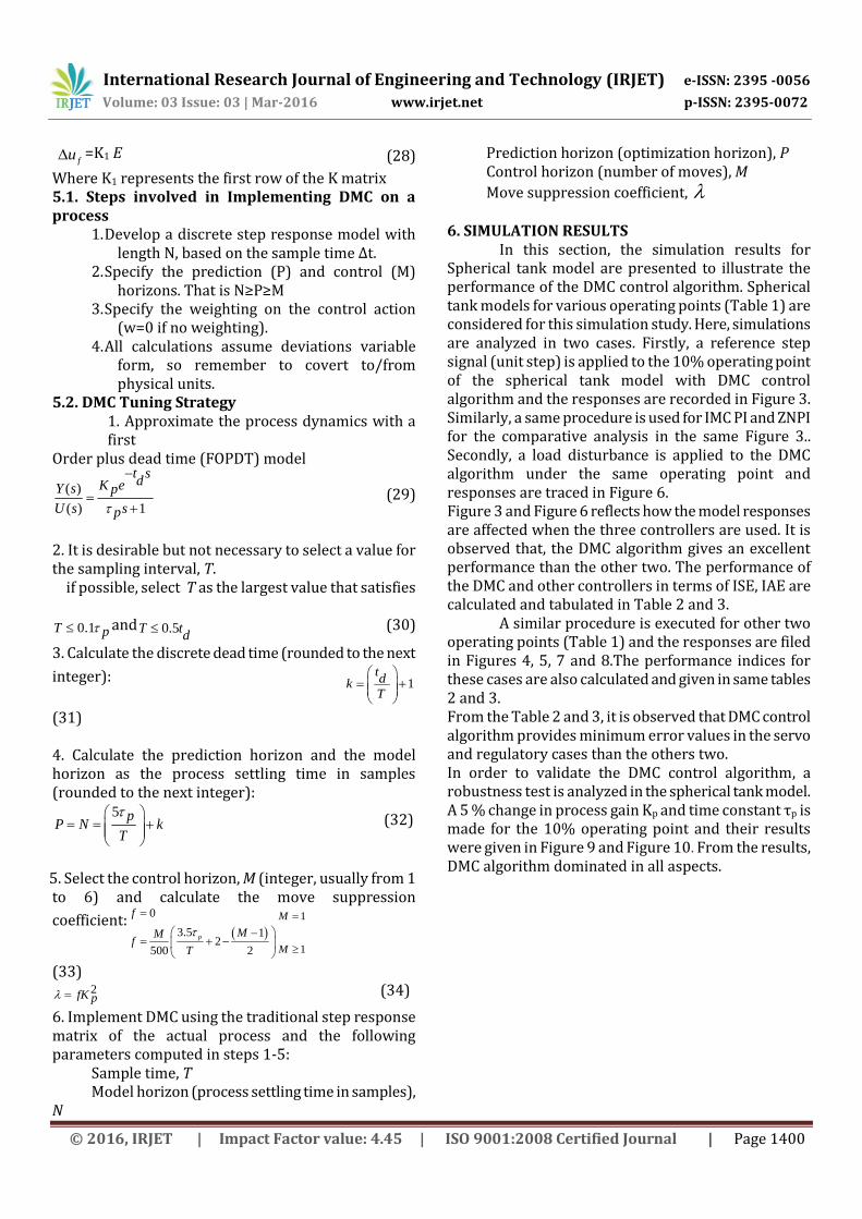
In this section, the simulation results for Spherical tank model are presented to illustrate the performance of the DMC control algorithm. Spherical tank models for various operating points (Table 1) are considered for this simulation study. Here, simulations are analyzed in two cases. Firstly, a reference step signal (unit step) is applied to the 10% operating point of the spherical tank model with DMC control algorithm and the responses are recorded in Figure 3. Similarly, a same procedure is used for IMC PI and ZNPI for the comparative analysis in the same Figure 3.. Secondly, a load disturbance is applied to the DMC algorithm under the same operating point and responses are traced in Figure 6. Figure 3 and Figure 6 reflects how the model responses are affected when the three controllers are used. It is observed that, the DMC algorithm gives an excellent performance than the other two. The performance of the DMC and other controllers in terms of ISE, IAE are calculated and tabulated in Table 2 and 3.

A similar procedure is executed for other two operating points (Table 1) and the responses are filed in Figures 4, 5, 7 and 8.The performance indices for these cases are also calculated and given in same tables 2 and 3. From the Table 2 and 3, it is observed that DMC control algorithm provides minimum error values in the servo and regulatory cases than the others two. In order to validate the DMC control algorithm, a robustness test is analyzed in the spherical tank model. A 5 % change in process gain Kp and time constant τp is made for the 10% operating point and their results were given in Figure 9 and Figure 10. From the results, DMC algorithm dominated in all aspects.




0 500 1000 1500 2000 2500 30000

0.5

1

1.5

Time(sec)

Lev

el(cm

)

DMC

IMC PI

ZN PI

Step

Fig.-3:Comparison of servo responses for DMC, IMC

PI and ZN PI Controllers at 10% Operating Point

0 500 1000 1500 2000 2500 30000

0.2

0.4

0.6

0.8

1

1.2

1.4

1.6

1.8

Time(sec)

Lev

el(cm

)

DMC

IMC PI

ZN PI

Step

Fig.-4:Comparison of servo responses for DMC, IMC PI and ZNPI Controllers at 50% Operating Point

0 500 1000 1500 2000 2500 30000

0.2

0.4

0.6

0.8

1

1.2

1.4

1.6

1.8

Time(sec)

Lev

el(cm

)

DMC

IMC PI

ZN PI

Step

Fig-5:.Comparison of servo responses for DMC, IMC PI and ZNPI Controllers at 66% Operating Point

0 500 1000 1500 2000 2500 3000-0.3

-0.2

-0.1

0

0.1

0.2

0.3

0.4

0.5

Time(sec)

Lev

el(cm

)

DMC

IMC PI

ZN PI

Fig.-6: Comparison of regulatory responses for DMC,

IMC PI and ZNPI Controllers at 10% Operating Point

0 500 1000 1500 2000 2500 3000-0.4

-0.3

-0.2

-0.1

0

0.1

0.2

0.3

0.4

0.5

Time(sec)

Lev

el(cm

)

DMC

IMC PI

ZN PI

Fig.7:.Comparison of regulatory responses for DMC, IMC PI and ZNPI Controllers at 50% Operating Point

0 500 1000 1500 2000 2500 3000-0.4

-0.3

-0.2

-0.1

0

0.1

0.2

0.3

0.4

0.5

Time(sec)

Lev

el(cm

)

DMC

IMC PI

ZN PI

Fig.-8:.Comparison of regulatory responses for DMC,

IMC PI and ZNPI Controllers at 66% Operating Point




0 500 1000 1500 2000 2500 30000

0.2

0.4

0.6

0.8

1

1.2

1.4

1.6

1.8

Time(sec)

Lev

el(cm

)

DMC

IMC PI

ZN PI

Step

Fig.-9:.Comparison of DMC, IMC PI and ZNPI Controllers

with 5% Kp change at 66% Operating Point

0 500 1000 1500 2000 2500 30000

0.2

0.4

0.6

0.8

1

1.2

1.4

1.6

Time(sec)

Lev

el(cm

)

DMC

IMC PI

ZN PI

Step

Fig.-10:.Comparison of DMC, IMC PI and ZNPI Controllers

with 5% τpchange at 10% Operating Point

Table 2 Performance Indices of DMC, IMC PI and ZNPI

Controllers for all the three Operating points- Servo

Responses

ISE IAE

10% 50% 66% 10% 50% 66%

DMC 190.7 207.3 242.9 240.6 268.6 308.9

IMCPI 191.5 208.8 244.1 253.3 277.8 319.3

ZNPI 197.9 267.7 281.9 320 436.5 465.6

Table 3 Performance Indices of DMC, IMC PI and ZNPI

Controllers for all the three Operating points-

Regulatory Responses

ISE IAE

10% 50% 66% 10% 50% 66%

DMC 45.71 51.79 59.51 115.2 133 151.7

IMCPI 47.87 52.19 60.01 126.6 138.9 159.71

ZNPI 49.47 66.91 70.46 160 218.2 232.8

7. CONCLUSION

A Dynamic Matrix Controller (DMC) is applied in to a non linear spherical tank system. Simulation runs are carried out by considering the DMC algorithm, IMC PI and conventional ZN PI-mode in a closed loop. The results clearly indicate that the incorporation of DMC in the control loop in spherical tank system provides a superior tracking performance than the IMC PI and conventional PI mode. A robustness of the DMC is also analyzed.

REFERENCES Reference

[1] Ya-Gang Wang, Hui-He Shao, “Optimal tuning for

PIcontroller”, Automatica, vol.36, 2000,pp.147-152,.

[2] Ari Ingimundarson,ToreHagglund,“Performance

comparison between PID and dead-time

compensatingcontrollers”,Journal of Process

Control,vol.12, ,2002, pp.887 - 895.

[3] Ming Ge, Min-Sen Chiu, Qing_Guo Wang, “Robust

PIDcontroller design Via LMIapproach",Journal of

Processcontrol , vol .12, 2002, pp.3-13,.

[4] Anandanatarajan and M.Chidambaram.”Experimental

evaluation of a controller using variabletansformation on

ahemi-spherical tank level process”, Proceedings

of National Conference NCPICD , 2005, pp. 195-200,.

[5] Cutler, C. R.; Ramaker, D. L. Dynamic Matrix Control-A

ComputerControl Algorithm. Proc. JACC; San Francisco,

CA, 1980.

[6] Maurath, P. R.; Mellichamp, D. A.; Seborg, D. E.

PredictiveController Design for Single Input/Single Output

Systems Ind.Eng. Chem. Res., vol.27, 956,1988a.

[7] Ogunnaike, B. A. Dynamic Matrix Control: A

Nonstochastic,Industrial Process Control Technique with

ParallelsIn AppliedStatistics. Ind. Eng. Chem. Fundam.

Vol.25,1986, 712

[8] Rahul Shridhar and Douglas J. Cooper, A Tuning Strategy

for Unconstrained SISO Model Predictive Control, Ind.

Eng. Chem. Res.vol. 36,1997, pp.729-746

Documents

Implementation of Dynamic Matrix Control for Non-Linear system · 2016-04-23 · Implementation of Dynamic Matrix Control for Non-Linear system Ramesh.S1, ... coefficient for the