Implementation of B-Spline Based Finite Element … project will examine -Splines as the basis shaped functions in finite the use of B element ... 3.1.2 The Weak Form ... include R.L

Implementation of B-Spline Based Finite Element Analysis

for the Boundary-Value Problem

Andrew J. Marker

A project submitted to the faculty of

Brigham Young University in partial fulfillment of the requirements for the degree of

Master of Science

Michael A. Scott, Chair Richard J. Balling Norman L. Jones

Department of Civil and Environmental Engineering

Brigham Young University

December 2013

Copyright © 2013 Andrew Marker

All Rights Reserved

ABSTRACT

Implementation of B-Spline Based Finite Element Analysis for the Boundary-Value Problem

Andrew J. Marker Department of Civil and Environmental Engineering

Master of Science

This project will examine the use of B-Splines as the basis shaped functions in finite element (FE) analysis. The analysis will be applied to a boundary-value problem. A program will be written to verify that B-Spline finite element (BSFE) analysis accurately represents the boundary-value problem.

Keywords: b-splines, finite element

TABLE OF CONTENTS

LIST OF TABLES ............................................................................................................ vii

LIST OF FIGURES ........................................................................................................... ix

1 Introduction .................................................................................................................. 1

2 Background ................................................................................................................... 2

Finite Element Method .......................................................................................... 2

2.1.1 Basic Concept .................................................................................................. 3

B-Splines ............................................................................................................... 3

2.2.1 Basic Concept .................................................................................................. 4

2.2.2 Basis Functions ............................................................................................... 4

3 Methods ........................................................................................................................ 7

The Boundary Value Problem ............................................................................... 7

3.1.1 The Strong Form ............................................................................................. 7

3.1.2 The Weak Form ............................................................................................... 8

3.1.3 The Galerkin Form .......................................................................................... 8

3.1.4 Matrix Form .................................................................................................... 9

3.1.5 Local Element point of view ........................................................................... 9

MATLAB Program ............................................................................................... 9

3.2.1 Gaussian Quadrature ..................................................................................... 10

3.2.2 Basis Values and Derivatives ........................................................................ 10

v

3.2.3 Mapping from Local to Global...................................................................... 11

3.2.4 Error .............................................................................................................. 12

4 Results and Conclulsions ............................................................................................ 13

Discussion of Results .......................................................................................... 13

Sources of Error .................................................................................................. 17

Conclusions ......................................................................................................... 17

REFERENCES ................................................................................................................. 18

Appendix A. Plots of Solutions ........................................................................................ 19

vi

LIST OF TABLES

Table 4-1: Error for f(x) = 1 .............................................................................................. 15

Table 4-2: Error for f(x) = x .............................................................................................. 15

Table 4-3: Error for f(x) = x2 ............................................................................................ 16

vii

viii

LIST OF FIGURES

Figure 2-1: Bézier and B-Spline Curves ............................................................................. 4

Figure 2-2: Linear B-Spline Basis over Five Elements ..................................................... 5

Figure 2-3: Quadratic B-Spline Basis over Four Elements ................................................ 5

Figure 2-4: Cubic B-Spline Basis over Six Elements ......................................................... 6

Figure 4-1: f(x) = 1, n = 5 ................................................................................................. 13

Figure 4-2: Enlarged picture of f(x) = 1, n=5 ................................................................... 14

Figure 4-3: f(x) = 1, n = 5000 ........................................................................................... 14

Figure 4-4: Error for f(x) = x2 .......................................................................................... 16

ix

x

1 INTRODUCTION

The finite element method (FEM) has been widely used for engineering purposes since its

introduction in the 1940’s and 1950’s. The age of computers accelerated the use and understanding

of FEM. FEM requires the use of basis equations to approximate the function. Often piece-wise

continuous polynomials, LaGrange or Hermite polynomials, have been used as the basis functions

in FEM. B-splines offer an alternative basis that is continuous over the whole model. In interesting

application of B-Spline based FEM is iso-geometric analysis (IGA). B-Splines are used

extensively in computer modeling which allows for B-Splines to be a link between modeling and

analysis.

This project will examine the use of B-Splines as the basis shaped functions in FEM

analysis. The analysis will be applied to the boundary-value problem. A program was developed

to run FEM on the boundary-value problem with first, second, and third-order basis functions. The

error between the actual solution and the FEM results are calculated and compared with FEM

using Lagrange polynomials of the same order. The rate of convergence was also calculated and

used to determine the efficiency of B-Spline based FEM. This paper provides a brief overview of

the finite element method and B-Splines. It discusses the method of the project. The results will

be presented and discussed.

1

2 BACKGROUND

This section provides a brief introduction to the finite element method and b-splines. It is

meant to provide enough information for the reader to understand the project, and is certainly not

exhaustive. For each topic a brief history is given as well as an introduction to the basic idea.

Finite Element Method

The finite method is used today for many engineering applications. Much research has and

continues to be devoted to this topic because of its importance in engineering analysis, although

the finite element method is relatively new. Its origins are in the 1940’s and 1950’s when

mathematicians and engineers were looking to solve high order problems with new numerical

methods. First publications on the subject include R.L. Courant’s Variational Methods for the

Solution of Problems of Equilibrium and Vibration in which he used piece-wise linear

approximations on triangles. The method is more clearly outlined by Argyris and Turner with

others in the 1950’s. The technique was first applied to the discipline of structures but found other

uses including heat conduction and fluids in the 1960’s. The development of computers has

increased the amount of research and application of the FEM. (Pepper, Heinrich, 2006, ). “Along

with the development of high-speed digital computers, the application of the finite element method

also progressed at a very impressive rate” (Rao, 2001). FEM continues to be a highly regarded and

used numerical method in engineering and other disciplines. Research continues in order find new

techniques and applications.

2

2.1.1 Basic Concept

The finite element method (FEM) is a numerical method. Like all numerical methods, the

idea is to find an approximation to a complex problem by replacing it with a simpler one. The idea

behind FEM is to break up a larger geometry into smaller sub-geometries, or elements. Analysis

of the individual elements can be completed based on the governing equations of the problem.

Approximations are made by linear combinations of the basis functions. The results are than

assembled into a global solution which approximates the real solution. The approximation

improves as the mesh is refined, that is as the number of elements increases. Different techniques

or greater computational effort can also be applied to FEM to create closer approximations.

(Huebner 2001, Reddy, 1984)).

B-Splines

Similar to the finite element method, the history of B-splines (basis splines) is relatively

new. . B-splines were first introduced for use in statistical data smoothing by Schoenberg in 1946

who coined the phrase. B-splines were developed for the automotive industry in the 1960’s as an

easy way to model the complex curves as found on automobiles. Two French mathematicians,

Bézier with Renault and De Casteljau’s with Citroën, simultaneously developed B-splines for

geometric design. There are two important mathematical developments in the history of B-splines.

First is the development of the recursive relation for defining and evaluating B-splines basis

functions. This is often credited to de Boor et al. The second is the creation of the polar form by

Ramshaw which allows for quick understanding and manipulating of B-splines. Today B-splines

3

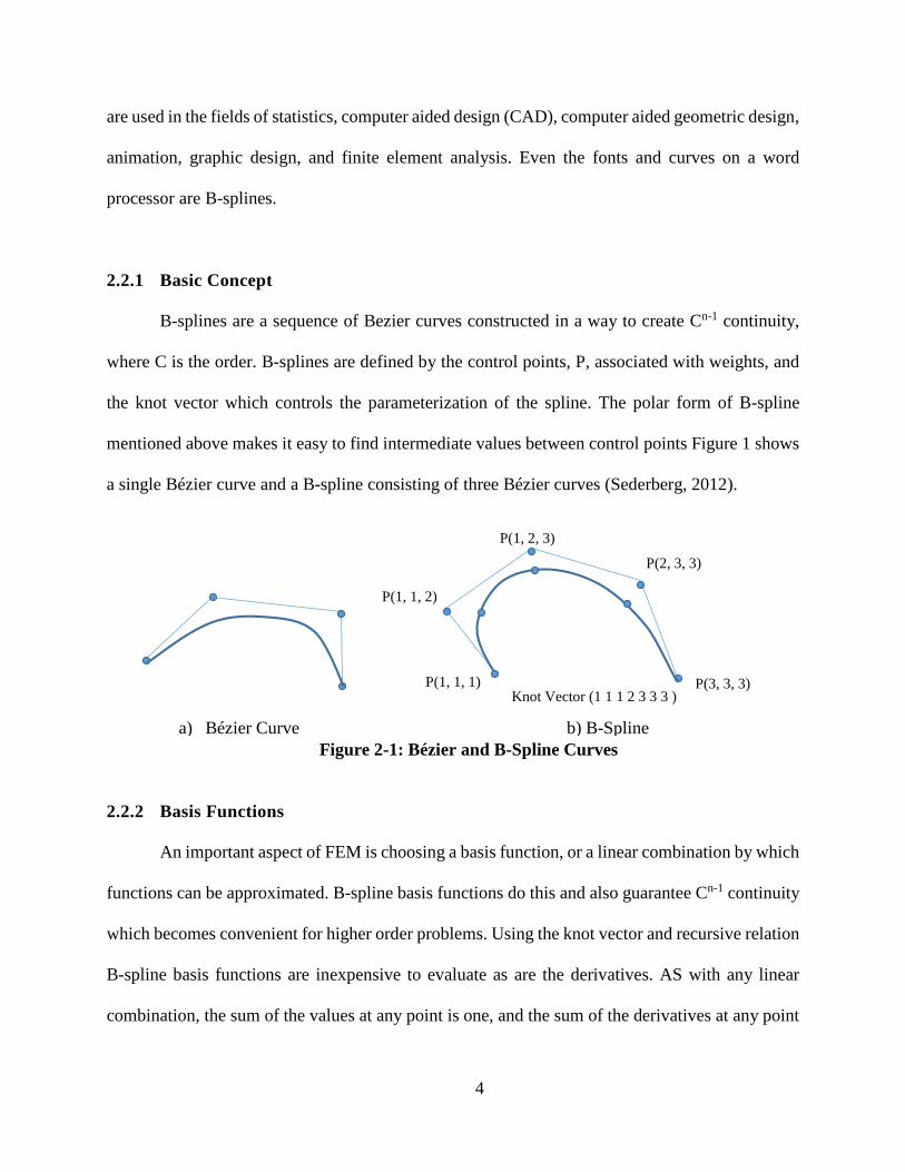
P(1, 1, 1)

P(1, 1, 2)

P(1, 2, 3)

P(2, 3, 3)

P(3, 3, 3) Knot Vector (1 1 1 2 3 3 3 )

b) B-Spline a) Bézier Curve Figure 2-1: Bézier and B-Spline Curves

are used in the fields of statistics, computer aided design (CAD), computer aided geometric design,

animation, graphic design, and finite element analysis. Even the fonts and curves on a word

processor are B-splines.

2.2.1 Basic Concept

B-splines are a sequence of Bezier curves constructed in a way to create Cn-1 continuity,

where C is the order. B-splines are defined by the control points, P, associated with weights, and

the knot vector which controls the parameterization of the spline. The polar form of B-spline

mentioned above makes it easy to find intermediate values between control points Figure 1 shows

a single Bézier curve and a B-spline consisting of three Bézier curves (Sederberg, 2012).

2.2.2 Basis Functions

An important aspect of FEM is choosing a basis function, or a linear combination by which

functions can be approximated. B-spline basis functions do this and also guarantee Cn-1 continuity

which becomes convenient for higher order problems. Using the knot vector and recursive relation

B-spline basis functions are inexpensive to evaluate as are the derivatives. AS with any linear

combination, the sum of the values at any point is one, and the sum of the derivatives at any point

4

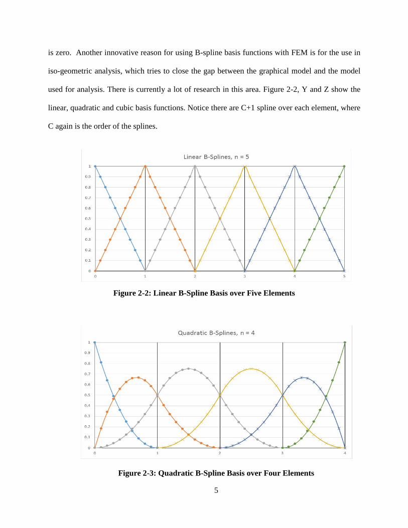
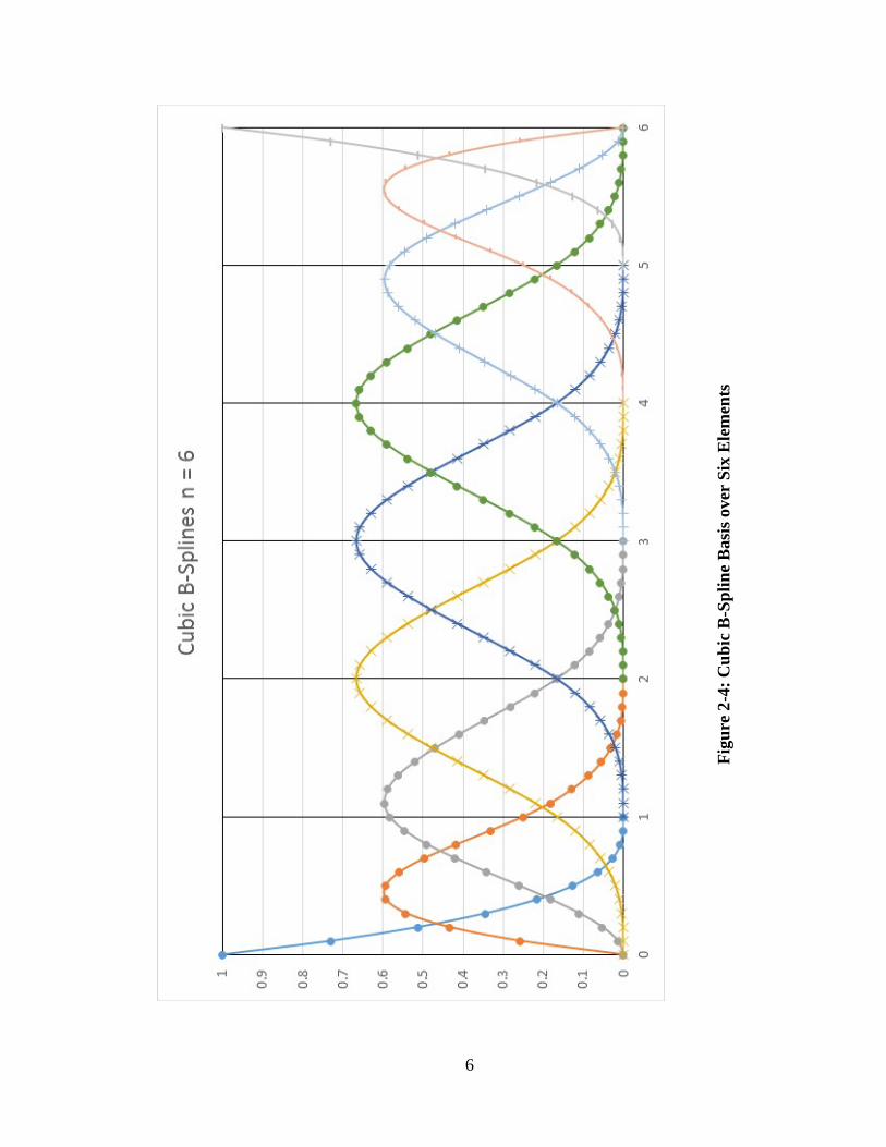
is zero. Another innovative reason for using B-spline basis functions with FEM is for the use in

iso-geometric analysis, which tries to close the gap between the graphical model and the model

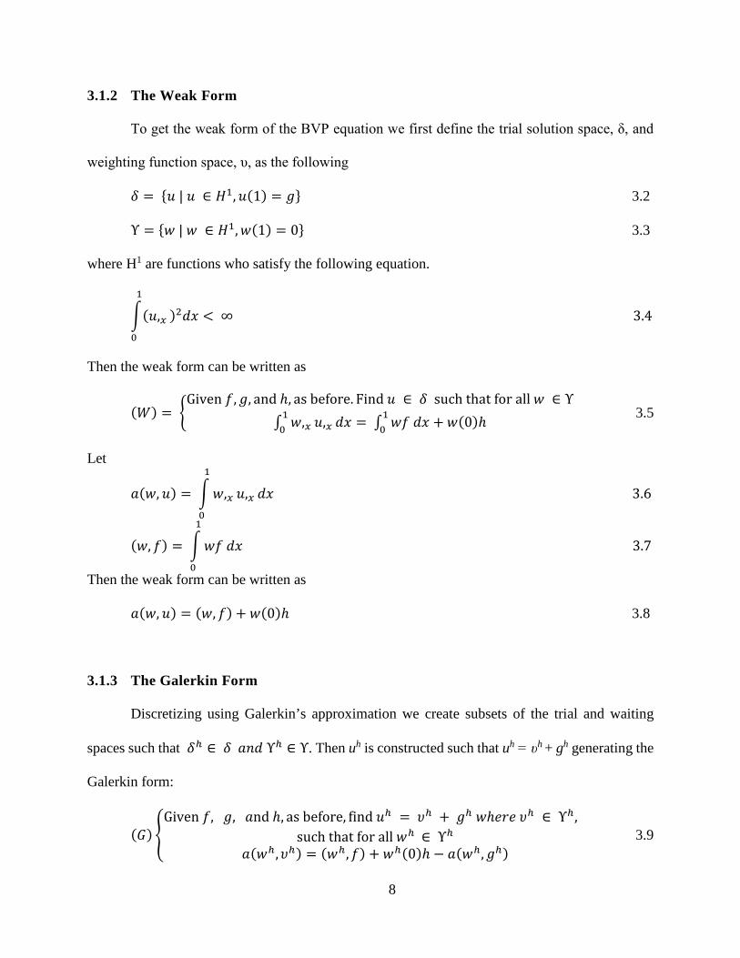
used for analysis. There is currently a lot of research in this area. Figure 2-2, Y and Z show the

linear, quadratic and cubic basis functions. Notice there are C+1 spline over each element, where

C again is the order of the splines.

Figure 2-2: Linear B-Spline Basis over Five Elements

Figure 2-3: Quadratic B-Spline Basis over Four Elements

5

Figu

re 2

-4: C

ubic

B-S

plin

e B

asis

ove

r Si

x E

lem

ents

6

3 METHODS

The purpose of this project was to implement a B-splines basis finite element program to

solve the boundary value problem. The main portion of the project consisted of defining the

problem, and solving the problem with a program in MATLAB. Also an Excel spreadsheet was

created and programmed to generate values for the basis function for a given order and number of

elements.

The Boundary Value Problem

The boundary value problem (BVP) has been widely studied as an introduction to finite

element method. It is a simple one dimensional first-order problem. It is introduced here briefly as

in Hughes (87) and can be studied in greater detail by referring to that book. The goal of the

following derivation is to get to a matrix form of the equation which is familiar and easy to solve.

3.1.1 The Strong Form

The strong or classical form of the BVP in terms of u on Ω = [0,1] is

(𝑆𝑆)

⎩⎨

⎧Given 𝑓𝑓 ∶ Ω → ℝ and constants 𝑔𝑔 and ℎ, find 𝑢𝑢 ∶ Ω → ℝ , 𝑠𝑠𝑢𝑢𝑠𝑠ℎ 𝑡𝑡ℎ𝑎𝑎𝑡𝑡

𝑢𝑢,𝑥𝑥𝑥𝑥+ 𝑓𝑓 = 0 𝑜𝑜𝑜𝑜 Ω𝑢𝑢(1) = 𝑔𝑔

−𝑢𝑢,𝑥𝑥 (0) = ℎ

3.1

where a comma represent differentiation and f is a function defined on Ω. The second and third

equations represent the boundary conditions. Both g and h are 0 for this project.

7

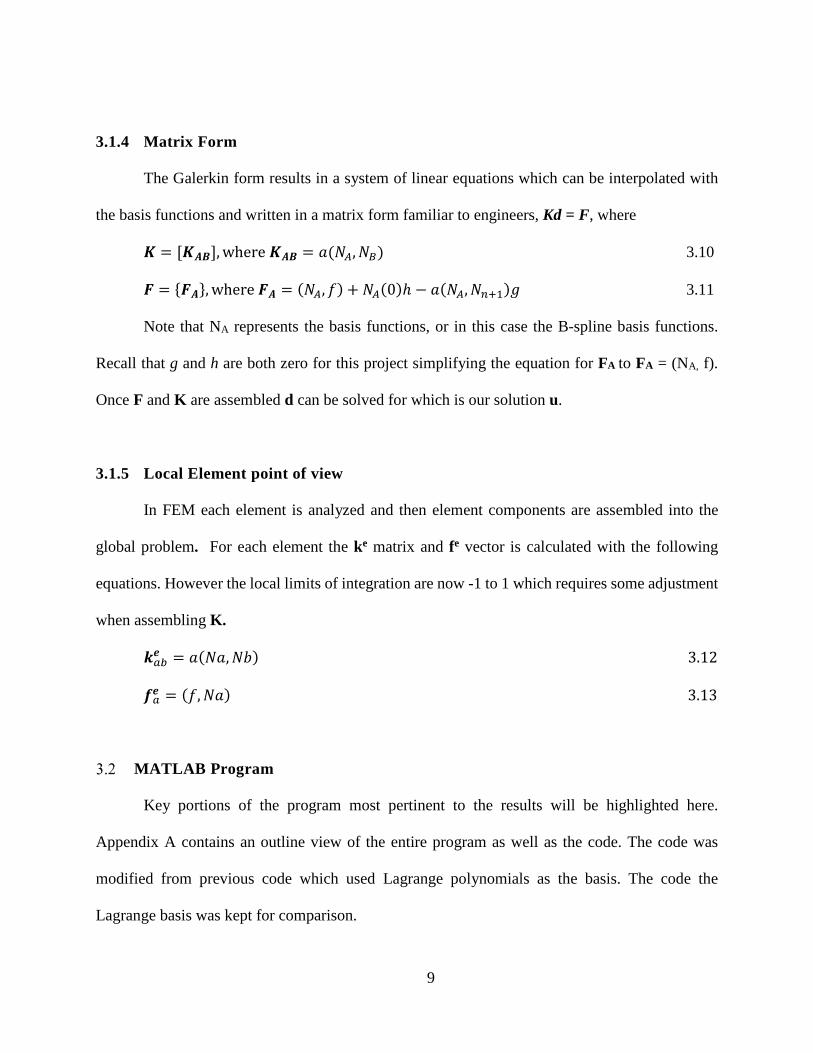
3.1.2 The Weak Form

To get the weak form of the BVP equation we first define the trial solution space, δ, and

weighting function space, υ, as the following

𝛿𝛿 = 𝑢𝑢 | 𝑢𝑢 ∈ 𝐻𝐻1,𝑢𝑢(1) = 𝑔𝑔 3.2

Υ = 𝑤𝑤 | 𝑤𝑤 ∈ 𝐻𝐻1,𝑤𝑤(1) = 0 3.3

where H1 are functions who satisfy the following equation.

(𝑢𝑢,𝑥𝑥 )2𝑑𝑑𝑑𝑑 < ∞ 3.41

0

Then the weak form can be written as

(𝑊𝑊) = Given 𝑓𝑓,𝑔𝑔, and ℎ, as before. Find 𝑢𝑢 ∈ 𝛿𝛿 such that for all 𝑤𝑤 ∈ Υ

∫ 𝑤𝑤,𝑥𝑥10 𝑢𝑢,𝑥𝑥 𝑑𝑑𝑑𝑑 = ∫ 𝑤𝑤𝑓𝑓 𝑑𝑑𝑑𝑑 + 𝑤𝑤(0)ℎ1

0 3.5

Let

𝑎𝑎(𝑤𝑤, 𝑢𝑢) = 𝑤𝑤,𝑥𝑥

1

0

𝑢𝑢,𝑥𝑥 𝑑𝑑𝑑𝑑 3.6

(𝑤𝑤,𝑓𝑓) = 𝑤𝑤𝑓𝑓 𝑑𝑑𝑑𝑑1

0

3.7

Then the weak form can be written as

𝑎𝑎(𝑤𝑤, 𝑢𝑢) = (𝑤𝑤,𝑓𝑓) + 𝑤𝑤(0)ℎ 3.8

3.1.3 The Galerkin Form

Discretizing using Galerkin’s approximation we create subsets of the trial and waiting

spaces such that 𝛿𝛿ℎ ∈ 𝛿𝛿 𝑎𝑎𝑜𝑜𝑑𝑑 Υℎ ∈ Υ. Then uh is constructed such that uh = υh + gh generating the

Galerkin form:

(𝐺𝐺)Given 𝑓𝑓, 𝑔𝑔, 𝑎𝑎nd ℎ, as before, find 𝑢𝑢ℎ = 𝜐𝜐ℎ + 𝑔𝑔ℎ 𝑤𝑤ℎ𝑒𝑒𝑒𝑒𝑒𝑒 𝜐𝜐ℎ ∈ Υℎ,

such that for all 𝑤𝑤ℎ ∈ Υℎ𝑎𝑎(𝑤𝑤ℎ, 𝜐𝜐ℎ) = (𝑤𝑤ℎ,𝑓𝑓) + 𝑤𝑤ℎ(0)ℎ − 𝑎𝑎(𝑤𝑤ℎ,𝑔𝑔ℎ)

3.9

8

3.1.4 Matrix Form

The Galerkin form results in a system of linear equations which can be interpolated with

the basis functions and written in a matrix form familiar to engineers, Kd = F, where

𝑲𝑲 = [𝑲𝑲𝑨𝑨𝑨𝑨], where 𝑲𝑲𝑨𝑨𝑨𝑨 = 𝑎𝑎(𝑁𝑁𝐴𝐴,𝑁𝑁𝐵𝐵) 3.10

𝑭𝑭 = 𝑭𝑭𝑨𝑨, where 𝑭𝑭𝑨𝑨 = (𝑁𝑁𝐴𝐴,𝑓𝑓) + 𝑁𝑁𝐴𝐴(0)ℎ − 𝑎𝑎(𝑁𝑁𝐴𝐴,𝑁𝑁𝑛𝑛+1)𝑔𝑔 3.11

Note that NA represents the basis functions, or in this case the B-spline basis functions.

Recall that g and h are both zero for this project simplifying the equation for FA to FA = (NA, f).

Once F and K are assembled d can be solved for which is our solution u.

3.1.5 Local Element point of view

In FEM each element is analyzed and then element components are assembled into the

global problem. For each element the ke matrix and fe vector is calculated with the following

equations. However the local limits of integration are now -1 to 1 which requires some adjustment

when assembling K.

𝒌𝒌𝑎𝑎𝑎𝑎𝒆𝒆 = 𝑎𝑎(𝑁𝑁𝑎𝑎,𝑁𝑁𝑁𝑁) 3.12

𝒇𝒇𝑎𝑎𝒆𝒆 = (𝑓𝑓,𝑁𝑁𝑎𝑎) 3.13

MATLAB Program

Key portions of the program most pertinent to the results will be highlighted here.

Appendix A contains an outline view of the entire program as well as the code. The code was

modified from previous code which used Lagrange polynomials as the basis. The code the

Lagrange basis was kept for comparison.

9

3.2.1 Gaussian Quadrature

Gaussian quadrature was used to evaluate the integrals in the analysis and in finding the

error. Gaussian quadrature works by taking a weighted sum of values at f at key integrations points.

𝑓𝑓(𝑑𝑑) ≈ 𝑓𝑓(𝜉𝜉𝑙𝑙) ∗ 𝑊𝑊𝑙𝑙

𝑛𝑛𝑖𝑖𝑖𝑖𝑖𝑖

𝑙𝑙=1

1

−1

3.14

It is an effective way to evaluate complicated integrals. Hughes reports that “accuracy of

order 2nint is gained by nint points of integration” (Hughes, 1987). A nint of 3 was used for this

project requiring that

𝜉𝜉1 = −3/5, 𝜉𝜉2 = 0, 𝜉𝜉3 = 3/5

W1 = W3 = 5/9, W2 = 8/9.

3.2.2 Basis Values and Derivatives

A large portion of the new code was to evaluate the new basis. Because Gaussian

quadrature was used to approximate the integrals, so the basis had to be evaluated at three points

in each element. With Lagrange polynomials the functions are the same over each element, so only

three points had to be evaluated. With the B-splines, three points for each element needed to be

calculated.

Using a uniform knot interval k:[0 0 0 1…n-1 n n n] for n elements, and the recursive

relation, the equations for the basis functions, and their derivatives can easily be evaluated at any

point. For example the quadratic formulas are

10

∈−−

−

∈

−

−−+

−−−

−

∈−−

−

=

++

++++

+

++

++

++

+

+

++

+

++

elsewhere

xxxxxxx

xx

xxxxx

xxxxxx

xxxxxx

xxxxxxx

xx

xB

iiiiii

i

iiii

ii

ii

ii

ii

iiiiii

i

i

,0

),[,))((

)(

),[,))(())((1

),[,))((

)(

)(

322313

23

2113

31

2

2

12

121

2

2 3.15

Where xi represent the knots. Functions were created that returned values and derivatives for each

of the basis equations.

3.2.3 Mapping from Local to Global

The element space is different than the global space due to the way the local element is

defined on [-1 1] and the global element is defined on [a b] where b –a = 1. To handle this apply a

change of variables to the local equations which result in a derivative term in the integral. In one

dimension this is related to the first derivative. Prior to integrating, the derivative term at each

quadrature point is determined as

𝑠𝑠𝑎𝑎𝑁𝑁𝑎𝑎(𝜉𝜉)𝐶𝐶+1

𝑎𝑎=1

3.16

Where ca are the control points of the B-Splines. For convenience the control point were chosen at

the greville abscissae so the geometric space and parametric space are equivalent.

11

3.2.4 Error

Error was calculated using a least squared approach. Again quadrature was applied for the

following integral. The rate of convergence, change in error per change in the number of elements

is a good indicator of how well a FEM is working.

𝐸𝐸 = (𝑢𝑢𝑎𝑎𝑎𝑎𝑡𝑡𝑡𝑡𝑎𝑎𝑙𝑙 − 𝑢𝑢𝑎𝑎𝑎𝑎𝑎𝑎𝑎𝑎𝑎𝑎𝑥𝑥 𝑑𝑑𝑢𝑢)1

0

1/2

3.17

12

4 RESULTS AND CONCLULSIONS

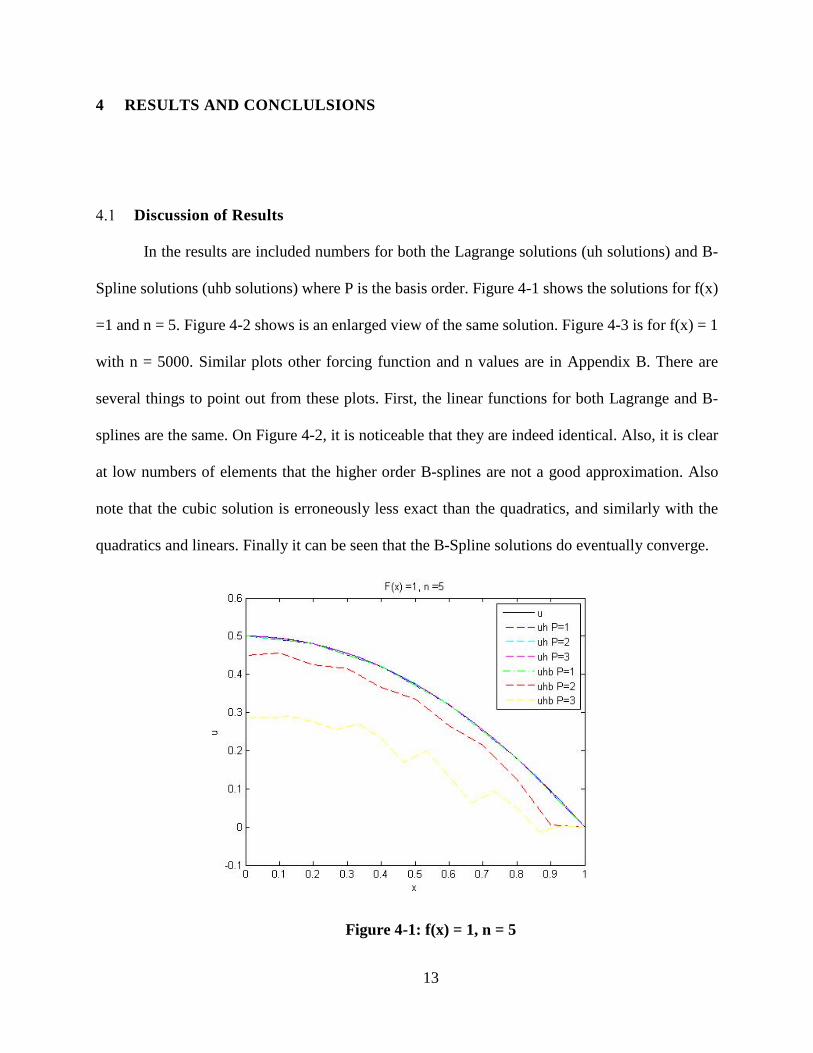
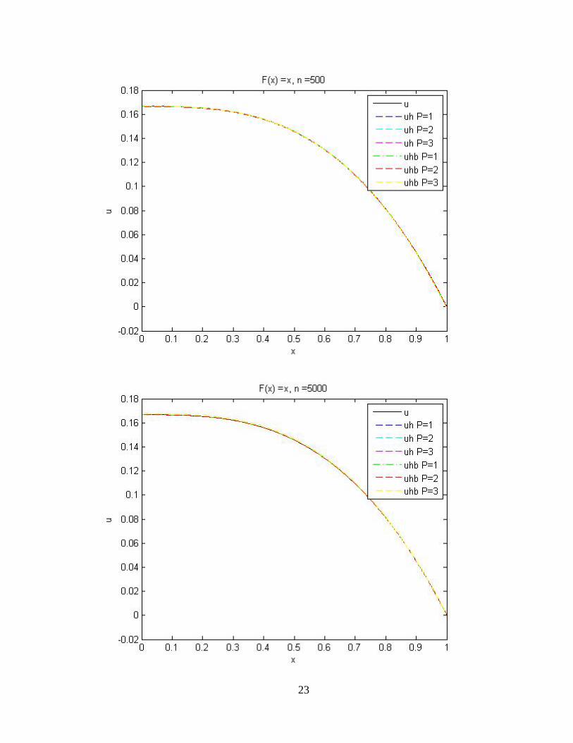
Discussion of Results

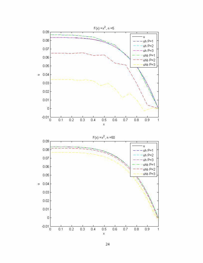
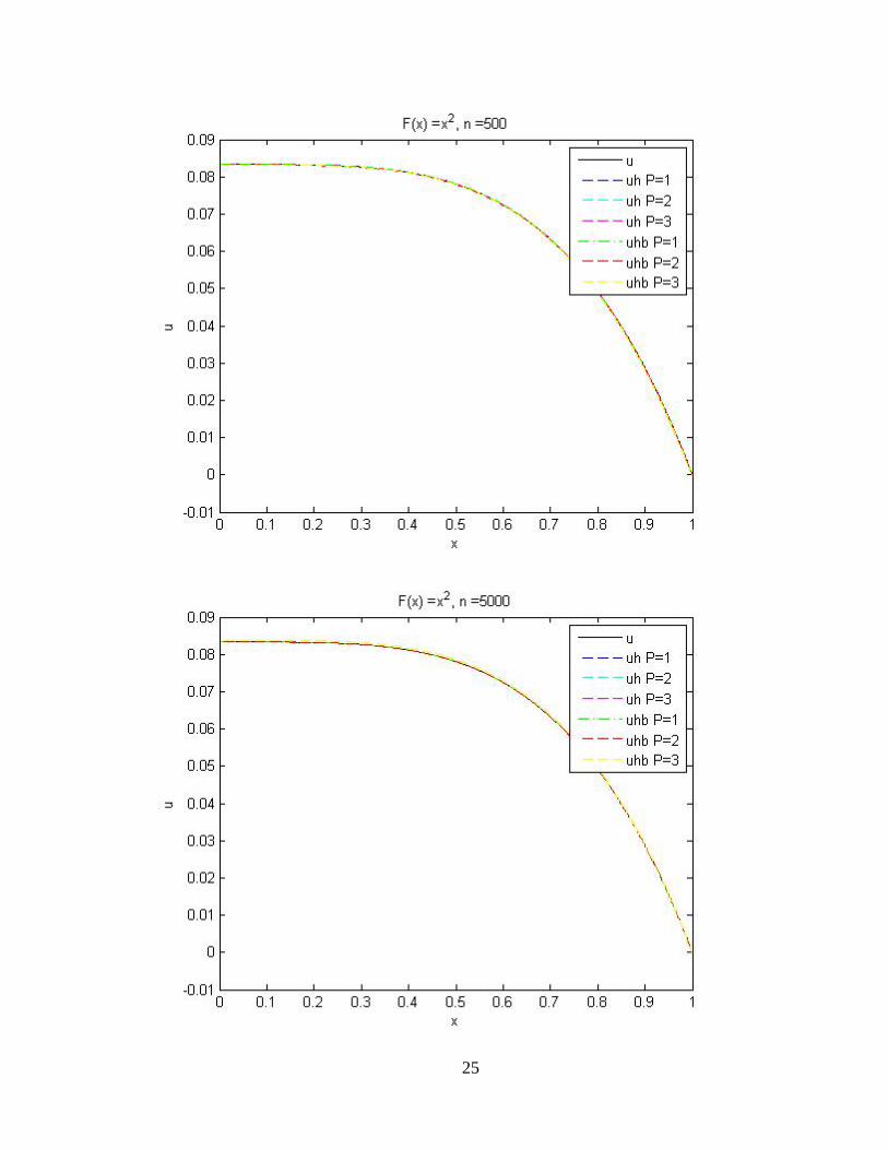
In the results are included numbers for both the Lagrange solutions (uh solutions) and B-

Spline solutions (uhb solutions) where P is the basis order. Figure 4-1 shows the solutions for f(x)

=1 and n = 5. Figure 4-2 shows is an enlarged view of the same solution. Figure 4-3 is for f(x) = 1

with n = 5000. Similar plots other forcing function and n values are in Appendix B. There are

several things to point out from these plots. First, the linear functions for both Lagrange and B-

splines are the same. On Figure 4-2, it is noticeable that they are indeed identical. Also, it is clear

at low numbers of elements that the higher order B-splines are not a good approximation. Also

note that the cubic solution is erroneously less exact than the quadratics, and similarly with the

quadratics and linears. Finally it can be seen that the B-Spline solutions do eventually converge.

Figure 4-1: f(x) = 1, n = 5

13

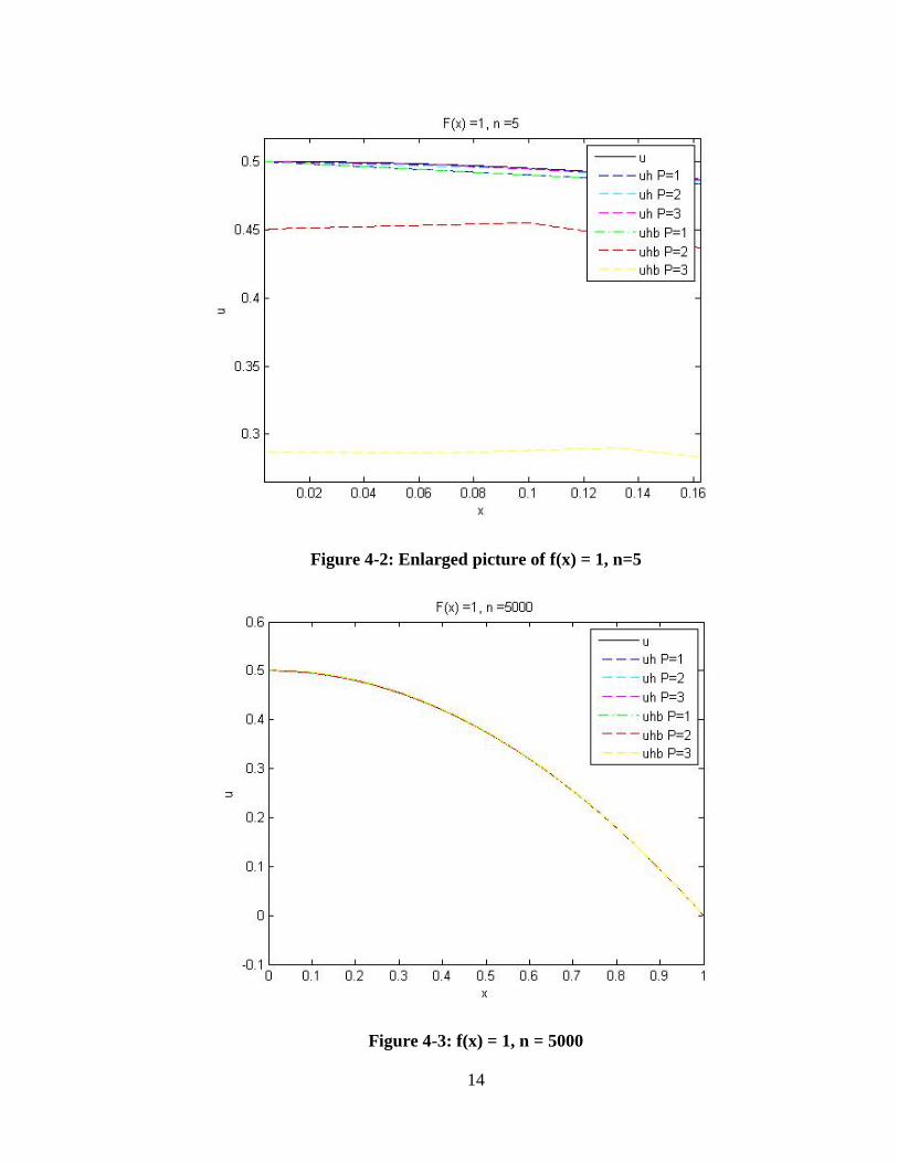
Figure 4-2: Enlarged picture of f(x) = 1, n=5

Figure 4-3: f(x) = 1, n = 5000

14

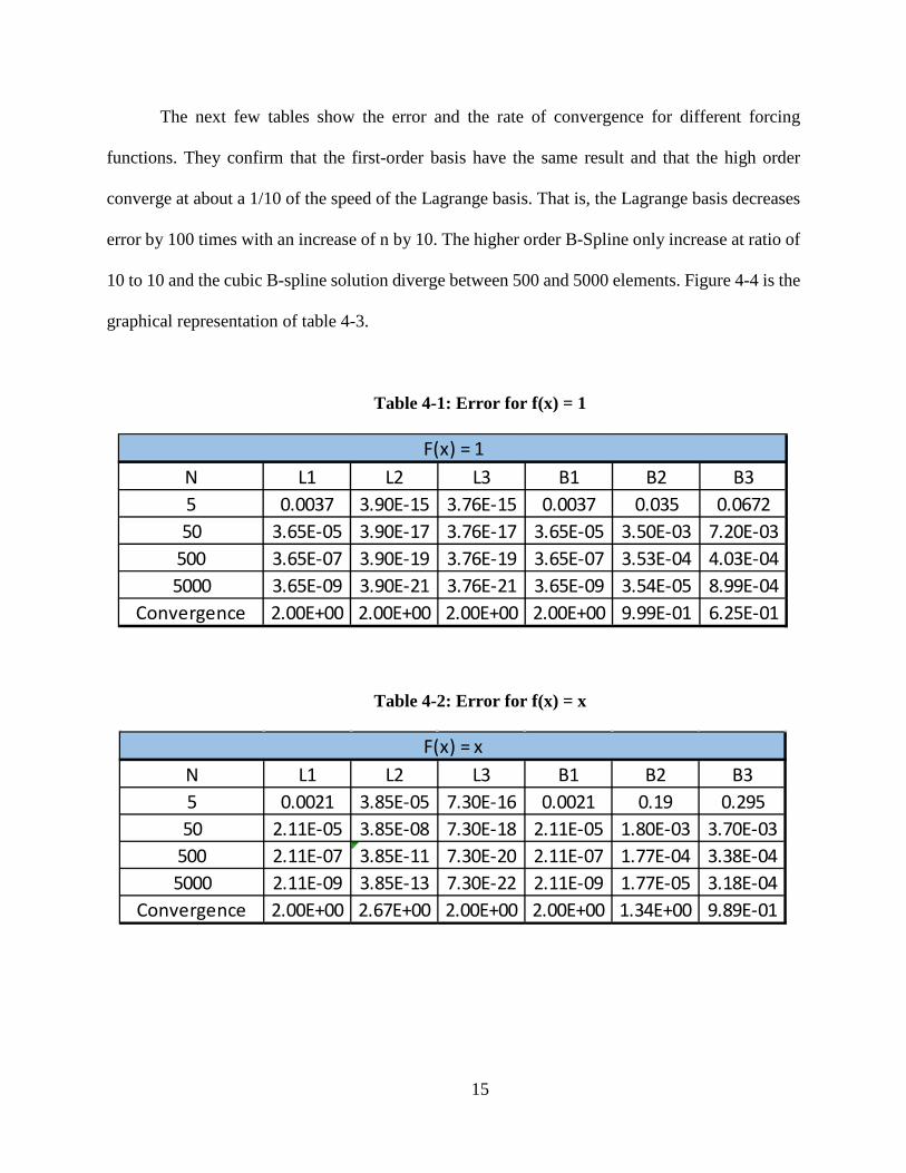
The next few tables show the error and the rate of convergence for different forcing

functions. They confirm that the first-order basis have the same result and that the high order

converge at about a 1/10 of the speed of the Lagrange basis. That is, the Lagrange basis decreases

error by 100 times with an increase of n by 10. The higher order B-Spline only increase at ratio of

10 to 10 and the cubic B-spline solution diverge between 500 and 5000 elements. Figure 4-4 is the

graphical representation of table 4-3.

Table 4-1: Error for f(x) = 1

Table 4-2: Error for f(x) = x

N L1 L2 L3 B1 B2 B35 0.0037 3.90E-15 3.76E-15 0.0037 0.035 0.067250 3.65E-05 3.90E-17 3.76E-17 3.65E-05 3.50E-03 7.20E-03

500 3.65E-07 3.90E-19 3.76E-19 3.65E-07 3.53E-04 4.03E-045000 3.65E-09 3.90E-21 3.76E-21 3.65E-09 3.54E-05 8.99E-04

Convergence 2.00E+00 2.00E+00 2.00E+00 2.00E+00 9.99E-01 6.25E-01

F(x) = 1


500 2.11E-07 3.85E-11 7.30E-20 2.11E-07 1.77E-04 3.38E-045000 2.11E-09 3.85E-13 7.30E-22 2.11E-09 1.77E-05 3.18E-04

Convergence 2.00E+00 2.67E+00 2.00E+00 2.00E+00 1.34E+00 9.89E-01

F(x) = x

15

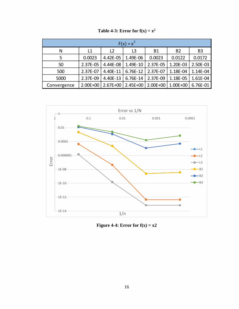
Table 4-3: Error for f(x) = x2

Figure 4-4: Error for f(x) = x2


500 2.37E-07 4.40E-11 6.76E-12 2.37E-07 1.18E-04 1.14E-045000 2.37E-09 4.40E-13 6.76E-14 2.37E-09 1.18E-05 1.61E-04

Convergence 2.00E+00 2.67E+00 2.45E+00 2.00E+00 1.00E+00 6.76E-01

F(x) = x2

1E-14

1E-12

1E-10

1E-08

0.000001

0.0001

0.01

10.00010.0010.010.11

Erro

r

1/n

Error vs 1/N

L1

L2

L3

B1

B2

B3

16

Sources of Error

While there are small errors that come from the approximations of the FEM, it is clear that

the results acquired here has more error than it should. It was briefly mentioned that there is a

difference between the local and global spaces. It is most likely that this large error is due to the

fact that the code does not properly account for mapping between the two spaces. The derivative

factor used to get the local into global get being incorrect or this mapping could be otherwise

missed in a different area.

Conclusions

The program written to implement a B-spline basis FEM was successful in the fact that it

created solutions that converged to the answer with mesh refinement (as the number of elements

increased). It was not successful as there is a large source of error, probably due to an issue

mapping between the two spaces, and because it converges too slowly. The program did not

successfully implement the B-spline basis. In order to make the program a success, the source of

error would need to be identified. Once the program worked for the boundary value problem, it

could than similarly be applied to higher order problems.

17

REFERENCES

Huebner, Kenneth H. 2001. The Finite Element Method for Engineers. 4th ed. New York: Wiley. Hughes, Thomas J.R. 1987. The Finite Element Method: Linear Static and Dynamic Finite

Element Analysis. Mineola, NY: Dover Publications. Pepper, Darrell W., and Juan C. Heinrich. 2006. The Finite Element Method: Basic Concepts and

Applications. 2nd ed. New York: Taylor & Francis. Rao, Singiresu S., 2011. The Finite Element Method in Engineering. 5th ed. Burlington, MA:

Butterworth-Heinemann. Reddy, J. N. 1984. An Introduction to the Finite Element Method. New York: McGraw-Hill. Sederberg, Thomas W. 2012. Computer Aided Geometric Design.

18

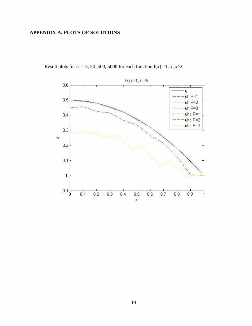
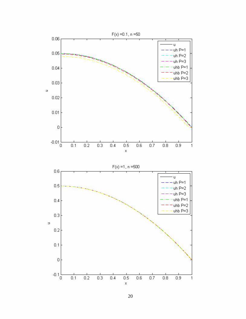
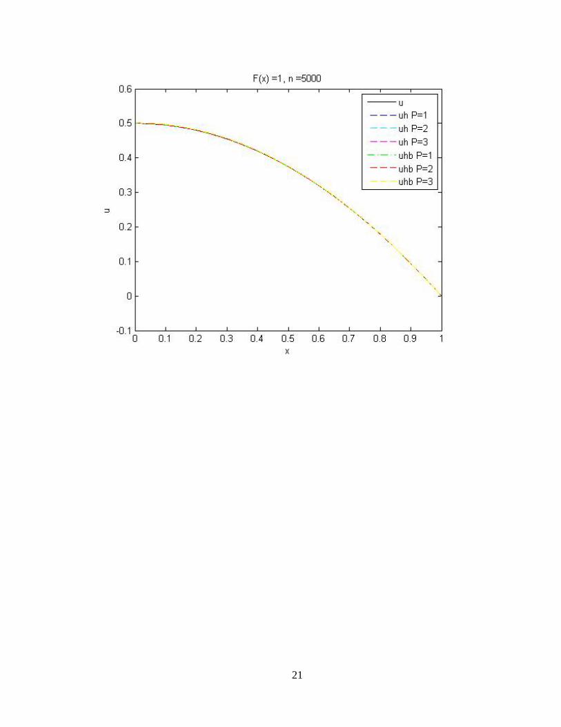
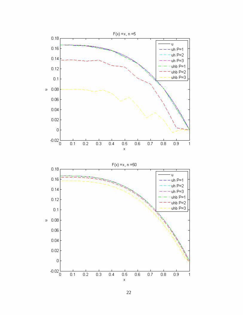
APPENDIX A. PLOTS OF SOLUTIONS

Result plots for n = 5, 50 ,500, 5000 for each function f(x) =1, x, x^2.

19

20

21

22

23

24

25

Documents

Implementation of B-Spline Based Finite Element … project will examine -Splines as the basis shaped functions in finite the use of B element ... 3.1.2 The Weak Form ... include R.L