Embed Size (px)
Citation preview
Imperfection sensitivity of thin-walled I-section struts susceptible
to cellular buckling
Li Bai, M. Ahmer Wadee∗
Department of Civil and Environmental Engineering, Imperial College London,
South Kensington Campus, London SW7 2AZ, UK
Abstract
A variational model that describes the nonlinear interaction between global and localbuckling of an imperfect thin-walled I-section strut under pure compression is developed.An initial out-of-straightness of the entire strut and an initial local out-of-plane displace-ment in the flanges are introduced as a global and a local type of imperfection respectively.A system of differential and integral equilibrium equations is derived for the structuralcomponent from variational principles, an approach that was previously validated. Im-perfection sensitivity studies focus on cases where the global and local critical loads aresimilar. Numerical results reveal that the strut exhibiting cellular buckling (or ‘snaking’) ishighly sensitive to both types of imperfections. The worst forms of local imperfection areidentified in terms of the initial wavelength, amplitude and degree of localization and thesechange with the generic imperfection size and highlight the potential dangers of unsafepredictions of actual load-carrying capacity.
Keywords: Structural stability; Mode interaction; Geometric imperfections; Snaking;Nonlinear mechanics.
1. Introduction
Thin-walled compression members made from metallic plate elements are susceptibleto a variety of buckling instability phenomena due to the high slenderness ratio at bothlocal and global scales [1, 2, 3]. It is also well known that when two buckling modes aretriggered in combination, the resulting behaviour is usually more unstable than when theyare triggered individually. In recent works [4, 5], an axially loaded thin-walled I-sectionstrut [6, 7, 8], made from a linear elastic material with an open and doubly-symmetriccross-section, was studied in detailed using an analytical approach. A variational modelrepresenting the nonlinear mode interaction between weak axis Euler buckling and theelastic local buckling of the flange plates was described. Other structural components suchas sandwich struts [9, 10, 11], stringer-stiffened and corrugated plates [12, 13, 14, 15, 16,
∗Corresponding authorEmail addresses: [email protected] (Li Bai), [email protected] (M. Ahmer Wadee)
Preprint submitted to International Journal of Mechanical Sciences October 19, 2015
17, 18] and thin-walled beams under uniform bending [19], are also known to suffer fromthe interaction of global and local modes of instability.
So-called ‘cellular buckling’ behaviour [20] or ‘snaking’ [21] was revealed in [4]. This hasbeen shown to occur where there are conflicting stabilities within the structural system.Currently, there is a trade-off between the strongly destabilizing effects of the local–globalbuckling mode interaction and the strongly stabilizing characteristics of pure local buck-ling. The mode interaction is known to manifest itself by exhibiting a localized bucklingprofile [10], whereas the stable local buckling shows a periodically distributed buckling pro-file. In combination, a progressive spreading of the initial interactively induced localizedbuckling mode within the flanges of the I-section strut is exhibited. This is characterizedby snap-backs in the equilibrium response showing sequential destabilization and restabi-lization, the graphs of which can resemble a snake (hence ‘snaking’) [22]. Moreover, thetransformation from localization to periodicity of the physical buckling profile occurs in aquasi-discrete manner with a buckling cell of deformation appearing with each snap-back,hence the term ‘cellular buckling’. The analytical model primarily focused on the perfectelastic post-buckling response and the results showed very good comparisons against ex-isting experimental and numerical works [23, 24], thus validating the approach. Moreover,systems exhibiting nonlinear mode interaction have been shown to be highly sensitive toboth global and local imperfections, where the most significant reduction in the ultimateload was observed when the global buckling load and the local buckling load are sufficientlyclose [1, 25, 23].
Previous studies on sandwich panels and struts on softening elastic foundations [26] re-vealed that local imperfections with different initial sizes and profiles may lead to differentbehaviours in terms of imperfection sensitivities. The current work extends the previousanalytical model [4] to study the behaviour of imperfect I-section struts. The two mostcommon types of imperfections are introduced, an initial out-of-straightness of the entirestrut and an initial local out-of-plane displacement of the flange plates, which are theninvestigated individually and in combination. The developed system of nonlinear ordinarydifferential equations subject to integral constraints is solved numerically using the con-tinuation and bifurcation software Auto-07p [27]. Examples are presented that revealthe severe imperfection sensitivities of the strut with the chosen geometries where globaland local buckling are, in turn, critical. Severe forms of local imperfection are identifiedin terms of the initial wavelength, amplitude and degree of localization. A discussion onthe implications of the findings is presented before the final conclusions are drawn togetherwith an outlook on future work.
2. Development of the analytical model
2.1. Modal description
Consider a thin-walled I-section strut of length L, made from a linear elastic, ho-mogeneous and isotropic material with Young’s modulus E and Poisson’s ratio ν. Thecoordinate system, section properties, local and global buckling modes are all shown inFigure 1. Note that currently the web thickness tw = 2t is assumed since the I-section is
2
(a) (b)
t
tw
b
y
t
L
P
z
y
h
θ(z)
W (z)z
x
Sway mode:
Tilt mode:
z
x
(c) (d)
x
y
w1w2
w2 w1
x
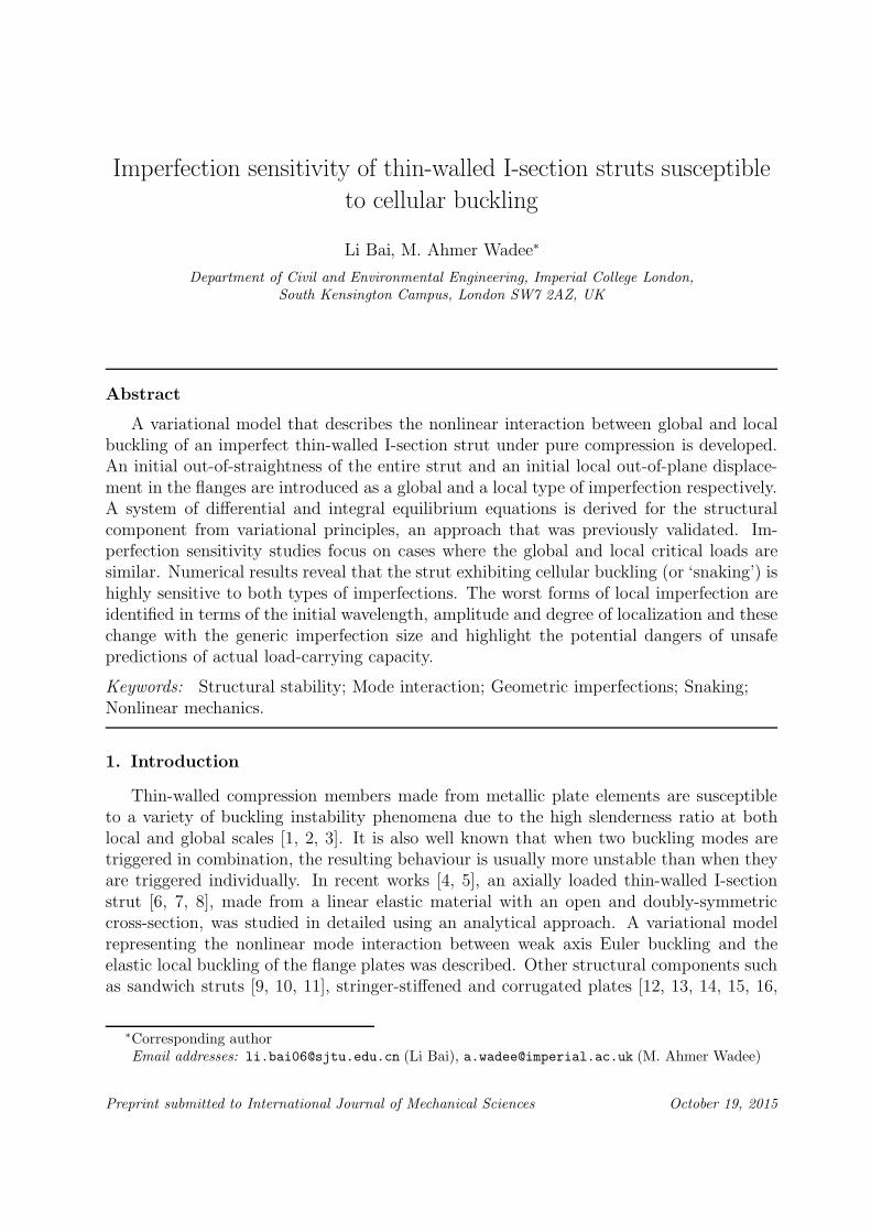
Figure 1: (a) Elevation of an I-section strut of length L that is compressed axially by a force P . Thelateral and longitudinal coordinates are y and z respectively. (b) Cross-section of strut with area A =2bt + (h − 2t)tw; the transverse coordinate is x. (c) Sway and tilt components of the weak axis globalbuckling mode. (d) Local buckling mode: out-of-plane flange displacement functions wi(x, z); note thelinear distribution of the displacement in the x-direction.
effectively composed from two C-shaped channel sections connected back-to-back, a typeof arrangement that has been used in previous experimental studies [23, 24, 4, 19]. In thissection, the previous model is extended to include an initial out-of-plane deflection in theflange plates as a type of local imperfection. The web is assumed to provide a simple sup-port to both flanges and not to buckle locally under axial compression. This assumptionof the flange–web joint having negligible rotational restraint has been shown to provide arealistically worst case scenario in terms of the severity of the post-buckling response [5].The strut length L is varied such that in one case, global buckling about the weaker y-axisoccurs before any flange buckles locally and in the other case the reverse is true – flangelocal buckling occurs first.
Figure 1(c) shows the the degrees of freedom known as ‘sway’ and ‘tilt’ [10]. Theyare introduced in combination to model the global mode in which the effect of shear isaccounted. The lateral displacement W and the rotation of the plane section θ duringglobal buckling are defined by the following expressions:
W (z) = qsL sinπz
L, θ(z) = qtπ cos
πz
L, (1)
where qs and qt are generalized coordinates defined as the amplitudes of sway and tiltrespectively. For the local buckling mode, the lateral displacement functions, w1 and w2
and the in-plane displacement functions, u1 and u2 are shown in Figure 1(d) and Figure
3
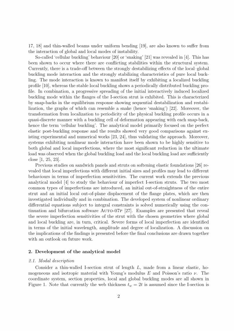
2, respectively. A linear distribution is assumed in the x-direction [28] for both wi and ui,
Web line
b/2 w1
Free edge
w2Free edge
b/2
w2(x, z) =2x
bw2(z)
w1(x, z) = −2x
bw1(z)
x
u2(0)
u1(0) Modelled flangeend-displacement
Average flangeend-displacement
z
u1(L)
u2(L)
Figure 2: Displacement functions of the local buckling mode in the flanges. Longitudinal and out-of-planeflange displacements ui(x, z) and wi(x, z) are defined respectively.
where i = {1, 2} throughout the current formulation. The linear distributions in the x-direction for ui reflect the assumption of Timoshenko beam theory. Moreover, the averageend-displacement, as opposed to the modelled flange end-displacement, is used to calculatethe local contribution to the work done by the external load.
2.1.1. Initial imperfections
An initial out-of-straightness in the x-direction, W0, and an initial rotation of the planesection θ0 are introduced to the web and the flanges respectively, as the global imperfection.The expressions for W0 and θ0, corresponding to Equation (1), are given by:
W0 = qs0L sinπz
L, θ0 = qt0π cos
πz
L. (2)
The local imperfection is introduced by defining an initial out-of-plane deflection, w0i(x, z),which has the form:
w0i(x, z) = (−1)i
(
2x
b
)
w0(z), (3)
where w0(z) is defined thus:
w0(z) = A0 sech[
α( z
L− η)]
cos[
βπ( z
L− η)]
(4)
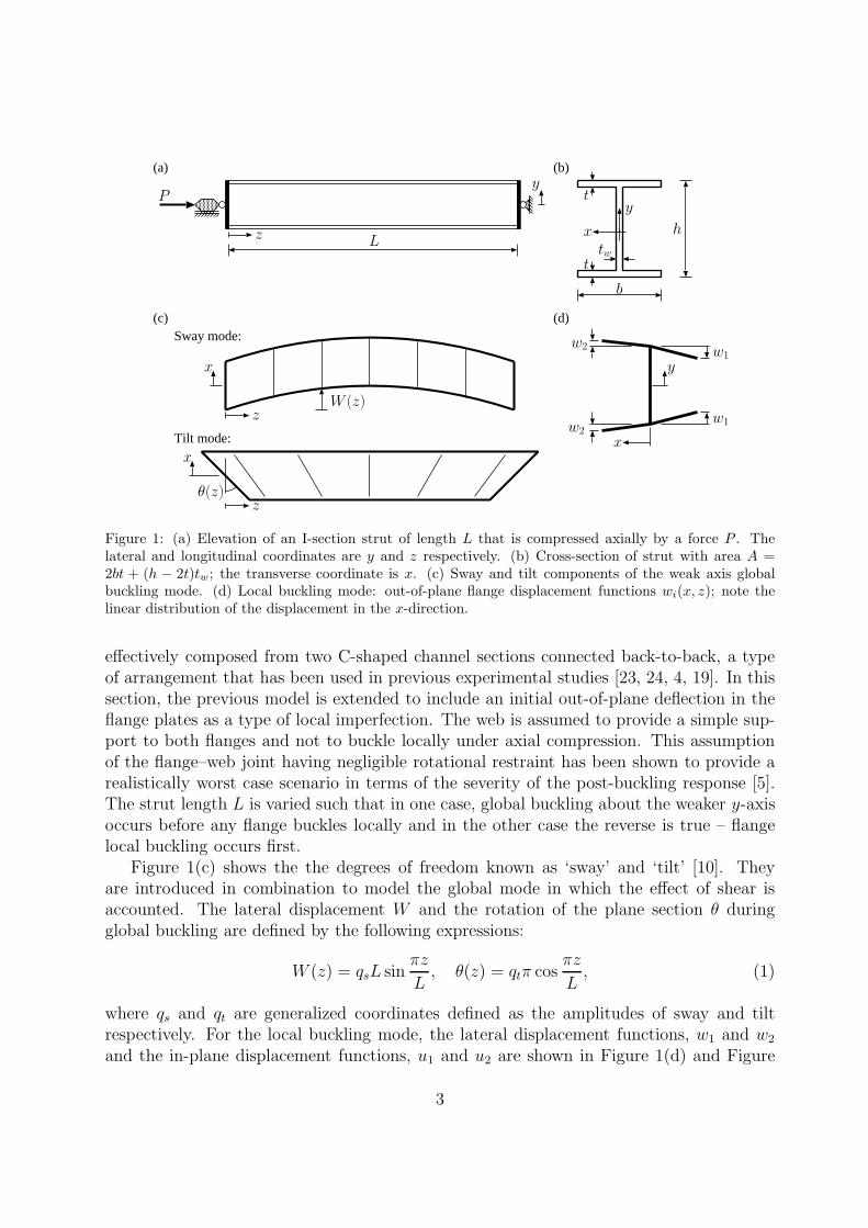
with z = [0, L] and the imperfection being symmetric about z/L = η. The value of ηis selected to be 1/2 because previous work on local–global mode interaction has demon-strated that the worst case occurs when the imperfection is symmetric about midspan [26].The distribution in the transverse direction x is assumed to be linear, which is consistentwith the definition of the local out-of-plane displacement wi(x, z). Note that A0 is theamplitude of the imperfection and β is the parameter that controls the number of waves
4

along the length in the imperfection. The parameter α controls the degree of localizationof the imperfection; it is periodic when α = 0, and modulated when α > 0. The quantitiesα and β are henceforth termed the ‘localization’ and ‘periodicity’ parameters respectively.The expression for w0 is a leading order approximation from a multiple scale perturbationanalysis of a strut on a nonlinear softening foundation, which closely matches the leaststable localized buckling mode shape [29]. This form of imperfection, illustrated in Figure3 for varying α and β, has been shown to be applicable to struts on a softening founda-
0 1 2−1
0
1
w0/A
0
2z/L
increasing α
(a)
0 1 2−1
0
1
w0/A
0
2z/L
increasing β
(b)
Figure 3: Local imperfection profile w0. (a) Localized imperfections introduced by increasing α. (b)Periodic imperfections (α = 0) with different numbers of half sine waves can be introduced by changingβ. In both cases η = 1/2.
tion and sandwich struts that undergo global and local buckling mode interaction [26]; thecurrent work adopts a similar approach.
2.2. Total potential energy
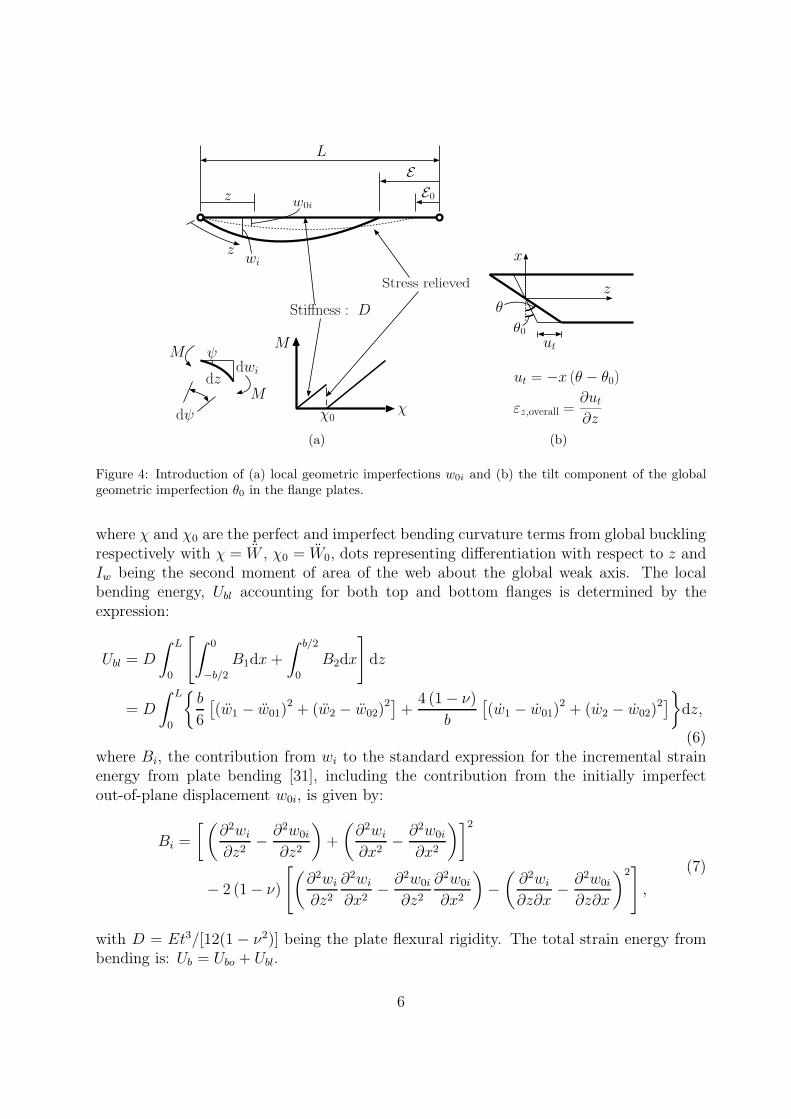
The procedure for deriving the total potential energy V of the perfect strut and thestrut with an initial global out-of-straightness W0 has been presented in previous work[4]. Similar to the global imperfection, the local imperfection is introduced by assumingthat the initial out-of-plane deflection w0 is stress-relieved [30, 26], implying that theelemental bending moment M and thus the local bending energy drops to zero when theinitial bending curvature χ = χ0, as illustrated in Figure 4(a). The local imperfections areintroduced to the more compressed flange with i = 1 and the less compressed flange withi = 2, respectively. Note that although w01 and w02 are identical after integration over theflange width, the notation cannot be used interchangeably in the case where global bucklingis critical. This is because the local buckling displacement in the less compressed half ofthe flange can be neglected (w02 = 0) since it was found in [4] that the less compressed halfof the flange rapidly flattens out due to the tensile stress components introduced from theglobal sway displacement W . However, when local buckling is critical, the imperfectioncan be introduced equally to each side of the flange and the resulting equations may besimplified by imposing the condition |w01| = |w02|.
The global bending energy (Ubo) is given by the following expression:
Ubo =1
2EIw
∫ L
0
(χ − χ0)2 dz =
1
2EIw
∫ L
0
(qs − qs0)2 π4
L2sin2
πz
Ldz, (5)
5
ψ
L
E
E0z
wi
w0i
Stiffness : D
z
dψ
dzdwi
M
M
M
χχ0
Stress relieved
(a)
θ0
θ
z
x
εz,overall =∂ut
∂z
ut = −x (θ − θ0)
ut
(b)
Figure 4: Introduction of (a) local geometric imperfections w0i and (b) the tilt component of the globalgeometric imperfection θ0 in the flange plates.
where χ and χ0 are the perfect and imperfect bending curvature terms from global bucklingrespectively with χ = W , χ0 = W0, dots representing differentiation with respect to z andIw being the second moment of area of the web about the global weak axis. The localbending energy, Ubl accounting for both top and bottom flanges is determined by theexpression:
Ubl = D
∫ L
0
[
∫
0
−b/2
B1dx +
∫ b/2
0
B2dx
]
dz
= D
∫ L
0
{
b
6
[
(w1 − w01)2 + (w2 − w02)
2]
+4 (1 − ν)
b
[
(w1 − w01)2 + (w2 − w02)
2]
}
dz,
(6)where Bi, the contribution from wi to the standard expression for the incremental strainenergy from plate bending [31], including the contribution from the initially imperfectout-of-plane displacement w0i, is given by:
Bi =
[(
∂2wi
∂z2−
∂2w0i
∂z2
)
+
(
∂2wi
∂x2−
∂2w0i
∂x2
)]2
− 2 (1 − ν)
[
(
∂2wi
∂z2
∂2wi
∂x2−
∂2w0i
∂z2
∂2w0i
∂x2
)
−
(
∂2wi
∂z∂x−
∂2w0i
∂z∂x
)2]
,
(7)
with D = Et3/[12(1 − ν2)] being the plate flexural rigidity. The total strain energy frombending is: Ub = Ubo + Ubl.
6

The membrane strain energy (Um) is derived from considering the longitudinal compo-nent of the direct strains (εzi) and the shear strains (γxzi) in the flanges. The direct strainsin the more and less compressed halves of the flanges, denoted as εz1 and εz2 respectively,are given by the generic direct strain εzi, namely:
εzi =∂ut
∂z− ∆ +
∂ui
∂z+
1
2
[
(
∂wi
∂z
)2
−
(
∂w0i
∂z
)2]
= x (qt − qt0)π2
Lsin
πz
L− ∆ + (−1)i
(
2x
b
)
ui +2x2
b2
(
w2
i − w2
0i
)
,
(8)
where ut = −(θ − θ0)x, which is essentially the in-plane displacement distribution fromthe tilt component of the global buckling mode, as shown in Figure 4(b). The local modecontribution is based on von Karman plate theory and a purely in-plane compressive straincomponent ∆ is also included. The membrane energy obtained from the direct strains (Ud),assuming that h ≫ t, is thus:
Ud = Et
∫ L
0
[
∫
0
−b/2
ε2
z1dx +
∫ b/2
0
ε2
z2dx
]
dz
= Etb
∫ L
0
{
b2
12(qt − qt0)
2 π4
L2sin2
πz
L− (qt − qt0)
bπ2
2Lsin
πz
L
[
1
3(u1 − u2)
+1
8
(
w2
1− w2
01
)
−1
8
(
w2
2− w2
02
)
]
+
(
1 +h
b
)
∆2 +1
6
(
u2
1+ u2
2
)
+1
40
[
(
w2
1− w2
01
)2+(
w2
2− w2
02
)2]
−1
2∆ (u1 + u2) −
1
6∆(
w2
1− w2
01
)
−1
6∆(
w2
2− w2
02
)
+1
8u1
(
w2
1− w2
01
)
+1
8u2
(
w2
2− w2
02
)
}
dz.
(9)
Note that the transverse component of strain εxi is neglected since it has been shown thatit has no effect on the post-buckling behaviour of a long plate with three simply-supportededges and one free edge [12]. The shear strains in the more and less compressive side ofthe flanges, denoted as γxz1 and γxz2 respectively, are given by the following generic shearstrain γxzi, namely:
γxzi =∂
∂z(W − W0) − (θ − θ0) +
∂ui
∂x+
∂wi
∂z
∂wi
∂x−
∂w0i
∂z
∂w0i
∂x
= (qs − qt − qs0 + qt0) π cosπz
L+ (−1)i
(
2
b
)
ui +4x
b2(wiwi − w0iw0i) .
(10)
7
The membrane energy component from the shear strains (Us) is thus:
Us = Gt
∫ L
0
[
∫
0
−b/2
γ2
xz1dx +
∫ b/2
0
γ2
xz2dx
]
dz
= Gtb
{
(qs − qt − qs0 + qt0)2 π2 cos2
πz
L+
2
b2
[
u12 + u2
2 +1
3(w1w1 − w01w01)
2
+1
3(w2w2 − w02w02)
2 + u1 (w1w1 − w01w01) + u2 (w2w2 − w02w02)
]
− (qs − qt − qs0 + qt0)π
bcos
πz
L
[
2u1 − 2u2 + (w1w1 − w01w01)
− (w2w2 − w02w02)
]}
,
(11)
where the shear modulus G = E/[2(1+ ν)] for a homogeneous and isotropic material. Thetotal membrane strain energy is: Um = Ud + Us.
The work done by the axial load P is given by:
PE =P
2
∫ L
0
[
q2
sπ2 cos2
πz
L− (u1 + u2) + 2∆
]
dz, (12)
where E comprises the respective terms: the longitudinal displacement due to global buck-ling, the in-plane displacement due to local buckling and the initial end-shortening frompure compression. Note that the displacement due to local buckling is taken as the aver-age value between the maximum in-plane displacement in the more compressed outstandu1 and the maximum in-plane displacement in the less compressed outstand u2, which isillustrated in Figure 2. The final expression of the total potential energy, V is:
V = Ub + Um − PE . (13)
2.3. Equilibrium equations
The equilibrium equations are obtained by performing the calculus of variations on thetotal potential energy V following the well established procedure presented in previousworks [10, 19, 4]. The integrand of the total potential energy V can be expressed as theLagrangian (L) of the form:
V =
∫ L
0
L (wi, wi, wi, ui, ui, z) dz. (14)
The first variation of V is given by:
δV =
∫ L
0
[
∂L
∂wi
δwi +∂L
∂wi
δwi +∂L
∂wi
δwi +∂L
∂ui
δui +∂L
∂ui
δui
]
dz. (15)
To determine the equilibrium states, V must be stationary, which requires the first variationδV to vanish for any small change in wi and ui. Since δwi = d(δwi)/ dz, δwi = d(δwi)/ dz
8
and similarly δui = d(δui)/ dz, integration by parts allows the development of the Euler–Lagrange equations for wi and ui; these comprise fourth order nonlinear ordinary differ-ential equations (ODEs) for wi and second order nonlinear ODEs for ui. The system isnon-dimensionalized with respect to the non-dimensional spatial coordinate z, which isdefined as z = 2z/L. The out-of-plane displacement wi and in-plane displacement ui arealso rescaled as wi = 2wi/L and ui = 2ui/L respectively. Moreover, the non-dimensionalinitially imperfect local out-of-plane displacement, w0 is given by:
w0 = A0 sech
[
1
2α (z − 2η)
]
cos
[
1
2βπ (z − 2η)
]
, (16)
where A0 = 2A0/L. The nonlinear ODEs for the rescaled variables wi and ui are thus:
˜....wi − 6φ2 (1 − ν) ˜wi − (−1)i
(
3D
8
)
{
(qt − qt0)π2
4φ
(
sinπz
2˜wi +
π
2cos
πz
2˜wi
)
− (−1)i
[
˜wi
(
2
3∆ −
3
5˜w2
i
)
−1
2
(
˜ui˜wi + ˜ui
˜wi
)
]}
+3
40D ˜w0i
(
˜wi˜w0i + 2 ˜wi
˜w0i
)
−3G
8φ2wi
[
2
3˜w2
i +2
3wi
˜wi + ˜ui − (−1)i (qs − qt − qs0 + qt0)π2
2φsin
πz
2
]
+1
4Gφ2wi
(
˜w0iw0i + ˜w2
0i
)
= ˜....w0i − 6φ2 (1 − ν) ˜w0i,
(17)
˜ui +3
4˜wi
˜wi + (−1)i
{
(qt − qt0)π3
4φcos
πz
2−
(
3Gφ2
D
)
[
(qs − qt − qs0 + qt0)π
φcos
πz
2
+ (−1)i
(
1
2wi
˜wi + ui
)]}
=3
4˜w0i
˜w0i −3φ2G
2D˜w0iw0i,
(18)
where D = EtL2/D, G = GtL2/D, φ = L/b and dots now represent derivatives withrespect to z. Equilibrium also requires minimization of the total potential energy withrespect to the generalized coordinates qs, qt and ∆. These lead to three integral equations,
9
thus:
∂V
∂qs= π2 (qs − qs0) + s (qs − qt − qs0 + qt0) −
PL2
EIwqs
−sφ
2π
∫
2
0
cosπz
2
[
(u1 − u2) +1
2
(
w1˜w1 − w01
˜w01
)
−1
2
(
w2˜w2 − w02
˜w02
)
]
dz = 0,
∂V
∂qt= π2 (qt − qt0) − t (qs − qt − qs0 + qt0)
+φ
2
∫
2
0
{
t
2πcos
πz
2
[
(
w1˜w1 − w01
˜w01
)
−(
w2˜w2 − w02
˜w02
)
+ 2 (u1 − u2)
]
− sinπz
2
[
2(
˜u1 − ˜u2
)
+3
4
(
˜w2
1− ˜w2
01
)
−3
4
(
˜w2
2− ˜w2
02
)
]}
dz = 0,
∂V
∂∆=
∫
2
0
{(
1 +h
b
)
∆ −1
4
(
˜u1 + ˜u2
)
−1
12
[(
˜w2
1− ˜w2
01
)
+(
˜w2
2− ˜w2
02
)]
−P
2Etb
}
dz = 0,
(19)
where s = 2GtbL2/(EIw) and t = 12Gφ2/E. The following relationship between qs0 andqt0 is assumed:
qs0 =
(
π2
t+ 1
)
qt0, (20)
which corresponds to the relationship between qs and qt directly before any interactivebuckling takes place (wi = ui = 0). This simplifies the computations by reducing thenumber of parameters describing the global imperfection to one. The boundary conditionsfor wi and ui and their derivatives are for pinned end conditions at z = 0 and for symmetryat z = 1:
wi(0) = ˜wi(0) = ˜wi(1) =...wi(1) = ui(1) = 0. (21)
The boundary condition at z = 0 from matching the in-plane strains becomes:
1
3˜ui(0) +
1
8
[
˜w2
i (0) − ˜w2
0i(0)]
−1
2∆ +
P
2Etb= 0. (22)
Note that all the boundary conditions arise naturally from minimizing V [10].The global critical load PC
o , determined by linear eigenvalue analysis of the perfectsystem, is given by the following expression:
PC
o =π2EIw
L2+
2Gtb
1 + t/π2. (23)
Note that if the assumption of Euler–Bernoulli bending theory, rather than Timoshenkobending theory, were to be imposed, it would assume that shear strains from bending wouldbe negligible. Hence, the limit G → ∞ would be imposed and the expression for PC
o wouldreduce to the classical Euler load for strut buckling about the cross-section weak axis [31].
10
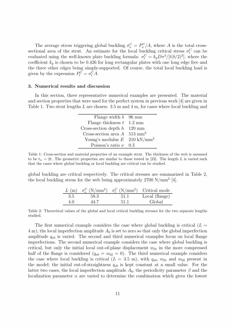
The average stress triggering global buckling σCo = PC
o /A, where A is the total cross-sectional area of the strut. An estimate for the local buckling critical stress σC
l can beevaluated using the well-known plate buckling formula: σC
l = kpDπ2/[t(b/2)2], where thecoefficient kp is chosen to be 0.426 for long rectangular plates with one long edge free andthe three other edges being simply-supported. Of course, the total local buckling load isgiven by the expression PC
l = σC
l A.
3. Numerical results and discussion
In this section, three representative numerical examples are presented. The materialand section properties that were used for the perfect system in previous work [4] are given inTable 1. Two strut lengths L are chosen: 3.5 m and 4 m, for cases where local buckling and
Flange width b 96 mmFlange thickness t 1.2 mm
Cross-section depth h 120 mmCross-section area A 513 mm2
Young’s modulus E 210 kN/mm2
Poisson’s ratio ν 0.3
Table 1: Cross-section and material properties of an example strut. The thickness of the web is assumedto be tw = 2t. The geometric properties are similar to those tested in [23]. The length L is varied suchthat the cases where global buckling or local buckling are critical can be studied.
global buckling are critical respectively. The critical stresses are summarized in Table 2,the local buckling stress for the web being approximately 2700 N/mm2 [4].
L (m) σC
o (N/mm2) σC
l (N/mm2) Critical mode3.5 58.3 51.1 Local (flange)4.0 44.7 51.1 Global
Table 2: Theoretical values of the global and local critical buckling stresses for the two separate lengthsstudied.
The first numerical example considers the case where global buckling is critical (L =4 m); the local imperfection amplitude A0 is set to zero so that only the global imperfectionamplitude qs0 is varied. The second and third numerical examples focus on local flangeimperfections. The second numerical example considers the case where global buckling iscritical, but only the initial local out-of-plane displacement w01 in the more compressedhalf of the flange is considered (qs0 = w02 = 0). The third numerical example considersthe case where local buckling is critical (L = 3.5 m), with qs0, w01 and w02 present inthe model; the initial out-of-straightness qs0 is kept constant at a small value. For thelatter two cases, the local imperfection amplitude A0, the periodicity parameter β and thelocalization parameter α are varied to determine the combination which gives the lowest
11
peak load for a given imperfection size; this is defined as the worst case combination forthe local imperfection.
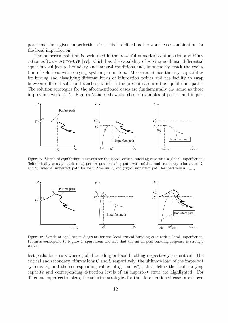
The numerical solution is performed in the powerful numerical continuation and bifur-cation software Auto-07p [27], which has the capability of solving nonlinear differentialequations subject to boundary and integral conditions and, importantly, track the evolu-tion of solutions with varying system parameters. Moreover, it has the key capabilitiesfor finding and classifying different kinds of bifurcation points and the facility to swapbetween different solution branches, which in the present case are the equilibrium paths.The solution strategies for the aforementioned cases are fundamentally the same as thosein previous work [4, 5]. Figures 5 and 6 show sketches of examples of perfect and imper-
P
qsqs0
Pu
P
wmax
Pu
wu
max
S
Imperfect path Imperfect path
P
qsqSs
Perfect path
PCo
SC PCo
PCo
qu
s
S
Figure 5: Sketch of equilibrium diagrams for the global critical buckling case with a global imperfection:(left) initially weakly stable (flat) perfect post-buckling path with critical and secondary bifurcations Cand S; (middle) imperfect path for load P versus qs and (right) imperfect path for load versus wmax.
P
wmax
PCl
A0
Pu
wu
max
Imperfect path
P
qs
Pu
Imperfect path
PCl
qu
s
P
Perfect path
PCl
S
C
wmax
Figure 6: Sketch of equilibrium diagrams for the local critical buckling case with a local imperfection.Features correspond to Figure 5, apart from the fact that the initial post-buckling response is stronglystable.
fect paths for struts where global buckling or local buckling respectively are critical. Thecritical and secondary bifurcations C and S respectively, the ultimate load of the imperfectsystems Pu and the corresponding values of qu
s and wu
maxthat define the load carrying
capacity and corresponding deflection levels of an imperfect strut are highlighted. Fordifferent imperfection sizes, the solution strategies for the aforementioned cases are shown
12

Increasing qs0 qs
P
Run 1
Run 2
PCo
(a)
Increasing w0
qs
P
Run 1
PCo
(b)
Increasing w0
qs
P
Run 1
qs0
PCl
(c)
Figure 7: Numerical continuation procedures for different imperfection sizes. (a) Global buckling beingcritical with initial out-of straightness qs0 only. (b) Global buckling being critical with initial local out-of-plane displacement w0 only. (c) Local buckling being critical with both qs0 and w0. The thicker linesshow the actual solution path in each of the examples shown. The thinner solid line shows the equilibriumpath of the perfect system. Circles represent bifurcation points.
diagrammatically in Figure 7. Note that it is only in the latter two cases that requirepurely a single run without branch switching. This is because in the case represented inFigure 7(b), where global buckling is critical, the local imperfection is introduced only tothe more compressed half of the flange (i = 1). This allows the break in symmetry as soonas the numerical run begins and therefore qs and qt are introduced without the need forbranch switching. In the case represented in Figure 7(c), where local flange buckling iscritical, although the local imperfections are introduced to both the more and less com-pressed halves of the flanges, the initial out-of-straightness W0 is also required such thatthe strut bends immediately as the load P is applied.
3.1. Global buckling critical: Global impefections (W0 6= 0, w01 = w02 = 0)
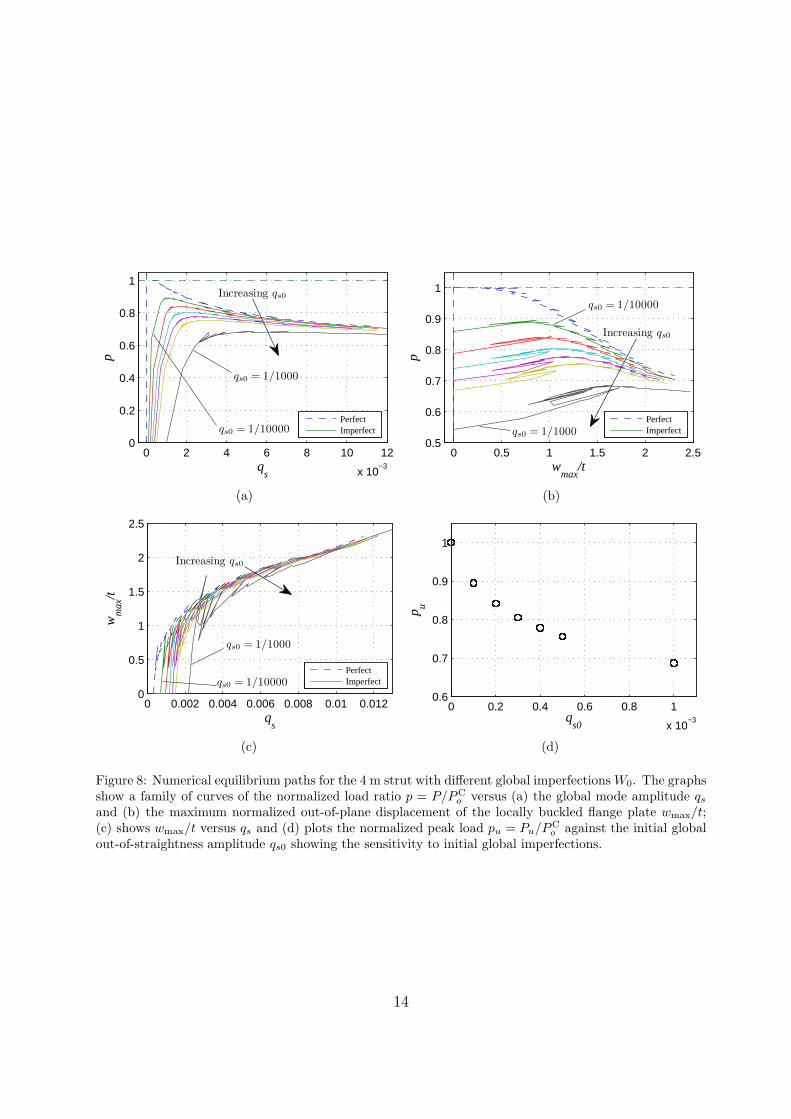
In this section, the strut with properties given in Table 1 with length L being 4 m isanalysed. Only an initial out-of-straightness W0 is introduced at this stage. A set of valuesof the initial out-of-straightness amplitude qs0 ranging from 1/10000 to 1/1000 is selectedfor analysis. Figure 8 shows a family of plots of the normalized axial load p = P/PC
o
versus (a) the global mode and (b) the local mode amplitudes; (c) shows the local andglobal mode relative magnitudes during post-buckling. Figure 8(d) shows a scatter plot ofthe normalized peak load, pu = Pu/P
C
o against the global imperfection amplitudes. It isclearly observed that the normalized peak load pu decreases as the size of the imperfectionincreases. A further inspection of the imperfection sensitivity plot in Figure 8(d) showsthat the peak load takes a significant drop as soon as a small imperfection is introduced.For qs0 = 1/1000, the peak load drops approximately 30% compared with the globalcritical load, PC
o of the perfect system, which shows that the strut is highly sensitive toglobal imperfections. Examining the post-buckling paths, where interactive buckling takesplace, it can be observed that the system converges to the same equilibrium state for all
13
0 2 4 6 8 10 12
x 10−3
0
0.2
0.4
0.6
0.8
1
qs
p
PerfectImperfect
Increasing qs0
qs0 = 1/1000
qs0 = 1/10000
(a)
0 0.5 1 1.5 2 2.50.5
0.6
0.7
0.8
0.9
1
wmax
/t
p
PerfectImperfect
Increasing qs0
qs0 = 1/10000
qs0 = 1/1000
(b)
0 0.002 0.004 0.006 0.008 0.01 0.0120
0.5
1
1.5
2
2.5
qs
wm
ax/t
PerfectImperfect
Increasing qs0
qs0 = 1/10000
qs0 = 1/1000
(c)
0 0.2 0.4 0.6 0.8 1
x 10−3
0.6
0.7
0.8
0.9
1
qs0
p u
(d)
Figure 8: Numerical equilibrium paths for the 4 m strut with different global imperfections W0. The graphsshow a family of curves of the normalized load ratio p = P/PC
oversus (a) the global mode amplitude qs
and (b) the maximum normalized out-of-plane displacement of the locally buckled flange plate wmax/t;(c) shows wmax/t versus qs and (d) plots the normalized peak load pu = Pu/PC
oagainst the initial global
out-of-straightness amplitude qs0 showing the sensitivity to initial global imperfections.
14
sizes of imperfection. As a result, struts with large global imperfections are expected tobe practically weakly stable (with Pu < PC
o ). It is worth noting that cellular bucklingbehaviour is captured for all sizes of imperfection [20, 19]. The final buckling mode shapeof the imperfect system is very similar to that of the perfect system in terms of bothamplitude and wavelength [4].
3.2. Global buckling critical: Local imperfections (w01 6= 0, W0 = w02 = 0)
In this section, the 4 m strut with a local imperfection only is analysed. The reducedset of equilibrium equations is solved and therefore the initial out-of-plane displacementw0 is only present in the more compressed half of the flange. The initial end-shorteningof the extreme fibre of the flange plate E0 (see Figure 4) due to the local imperfection, isdefined as:
E0 =1
2
∫ L
0
w2
0dz, (24)
which can also be considered as a kind of overall measure of the initial local imperfection[26]. Since A0, β and α are parameters that can have different combinations, this termprovides a direct interpretation of the size of the local imperfection, which is particularlyuseful in the imperfection sensitivity study to facilitate meaningful comparisons. The localimperfections are studied in three parts.
1. Parameters β and α are kept at constant values of 1 and 0 respectively with only A0
changing E0. This form of imperfection is essentially affine to the linear eigenvaluesolution for an axially loaded rectangular long plate with two short loaded edges andone long edge simply supported and the other long edge being free [28]. The peakloads Pu are recorded for each value of E0.
2. Periodic imperfections are investigated, where for each value of E0 selected, the valueof α = 0 and β is varied as the principal parameter. The amplitude, A0 is variedaccordingly to keep E0 at the selected value, with an increase in β resulting in acommensurate decrease in A0. Note that the value of β only takes odd integer valuesto satisfy the boundary and symmetry conditions. The combination of β and A0 thatgives the lowest peak load Pu for a given value of E0 is recorded.
3. Modulated local imperfections are investigated by varying α for each value of E0
selected. The amplitude, A0 is varied accordingly whereas β is kept at the value thatis determined in part 2. Generally, increasing α results in a higher value of A0. Thecombination of α and A0 that gives the lowest peak load Pu for a given value of E0
is recorded.
Figure 9 shows a series of imperfection sensitivity diagrams. It can be observed inFigure 9(a) that for β = 1 and α = 0, there is very little reduction in the peak load as E0
increases, indicating that the strut is fundamentally insensitive to this type of imperfectionin the elastic range. However, for the periodic imperfections with β varied, the peak loadsare reduced significantly as E0 increases. The periodicity parameter β that gives the lowestpeak load is different for each value of E0, which is shown in Figure 9(b). It is found that for
15

0 0.5 1 1.5
x 10−6
0.75
0.8
0.85
0.9
0.95
1
E0/L
p u
(a)
0 0.5 1 1.5
x 10−6
6
8
10
12
14
16
18
E0/L
β
(b)
0 0.5 1 1.5
x 10−6
0
2
4
6
8
E0/L
α
(c)
0 0.5 1 1.5
x 10−6
0
0.05
0.1
0.15
0.2
E0/L
A0/t
(d)
Figure 9: Imperfection sensitivity diagrams for the 4 m and 3.5 m struts with the abscissa in each casebeing the normalized local imperfection size E0/L plotted against: (a) the normalized peak load, pu, (b)the periodicity parameter β that gives the lowest peak loads, (c) the localization parameter α that gives thelowest peak loads and (d) the normalized imperfection amplitude A0/t. Triangle symbols denote resultsfor the 4 m strut with local imperfections affine to the plate local buckling eigenmode (α = 0, β = 1); “◦”and “+” symbols correspond to the periodic imperfection (β varying, α = 0) for the 4 m and 3.5 m strutsrespectively, whereas “×” and “∗” correspond to the modulated imperfection with α varying and β, asdetermined in (b), for the 4 m and 3.5 m struts respectively.
16
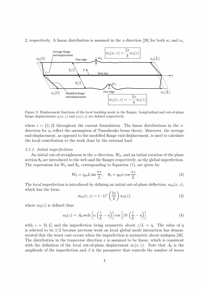
larger E0 values, periodic imperfections with larger wave numbers increase in prominence.A further reduction in the peak loads is observed when the imperfection is modulated, forall values of E0. The variation in the localization parameter α shows the opposite trend asin β – larger imperfections require less localization to give the most severe combination.It is observed in Figure 9(d) that for the largest E0 value in the graph, the amplitude A0
for the most severe periodic imperfection is more than t/10, whereas for the most severemodulated imperfection, A0 is slightly more than t/5. The reduction in the peak loads forthe periodic and modulated imperfections for the largest E0 is 11.8% and 12.6% respectively,indicating the strut is sensitive to both types of imperfection. Figure 10 shows the shapeof both periodic and modulated imperfections with the worst combination of A0, β and α,for each E0 value shown in the imperfection sensitivity diagrams.
Figure 11(a) shows a family of equilibrium paths for the worst case modulated imper-fections for all E0 values studied for the 4 m strut with local imperfections. Note that thenormalized total end shortening E/L is determined by the expression:
E
L=
q2
sπ2
4+
u1(0) + u2(0)
2L+ ∆, (25)
which was essentially given in Equation (12). A slightly different response is observedin contrast to the system with a global imperfection only. The number of snap-backs inthe equilibrium paths reduces as E0 increases. This is because the buckling mode shapestarts to develop from a smaller wavelength from the beginning, which is defined by theinitial imperfection. As a result, the formation of the first new peak or trough, from thecharacteristic cellular buckling snap-back, takes place further down the post-buckling pathfor larger initial imperfections. It is also observed that the formation of the new peak ortrough has a longer restabilization path, and therefore a larger snap-back, meaning thatmore membrane stretching is required for the formation of the new peak or trough.
3.3. Local buckling critical: Combined imperfections (W0 6= 0, |w01| = |w02| 6= 0)
In this section, the 3.5 m strut with both global and local imperfections is analysed.The global imperfection amplitude qs0 is kept at a nominal constant value of L/10000,whereas the local imperfections are introduced to the entire flange; therefore the full set ofthe equilibrium equations are solved. Figure 9 shows the imperfection sensitivity diagrams.Note that since the strut has been shown to be insensitive to the imperfection with β = 1,the focus is on the cases of periodic and modulated imperfections (study parts 2 and 3detailed in §3.2). The same E0 values are used as in the previous section. It is observedthat the strut is sensitive to both types of imperfections. However, although the modulatedimperfections always give lower peak loads than the periodic imperfections, the reductionis marginally less severe as compared with the L = 4 m case. For the largest E0 value, thereduction in the peak loads are 6.5% and 6.8% for the periodic and mdulated imperfectionsrespectively. In Figure 9(b), the most severe periodic imperfections for the L = 3.5 m strutare generally associated with shorter wavelengths. For the case of modulated imperfections,the degree of localization, which gives the worst combination, is approximately constantat α ≈ 4, which is quite different when compared to the L = 4 m strut, where the α drops
17
0 1000 2000 3000 4000
−0.2
0
0.2
w0 (
mm
)
z (mm)0 1000 2000 3000 4000
−0.2
0
0.2
w0 (
mm
)
z (mm)
0 1000 2000 3000 4000
−0.2
0
0.2
w0 (
mm
)
z (mm)0 1000 2000 3000 4000
−0.2
0
0.2
w0 (
mm
)z (mm)
0 1000 2000 3000 4000
−0.2
0
0.2
w0 (
mm
)
z (mm)0 1000 2000 3000 4000
−0.2
0
0.2
w0 (
mm
)
z (mm)
0 1000 2000 3000 4000
−0.2
0
0.2
w0 (
mm
)
z (mm)0 1000 2000 3000 4000
−0.2
0
0.2
w0 (
mm
)
z (mm)
0 1000 2000 3000 4000
−0.2
0
0.2
w0 (
mm
)
z (mm)0 1000 2000 3000 4000
−0.2
0
0.2
w0 (
mm
)
z (mm)
0 1000 2000 3000 4000
−0.2
0
0.2
w0 (
mm
)
z (mm)0 1000 2000 3000 4000
−0.2
0
0.2
w0 (
mm
)
z (mm)
Figure 10: Mode shapes of the initial out-of-plane displacement w0 showing the worst case combinationsof A0, β and α for the 4 m strut with increasing E0 values, shown in Figure 9, from top to bottom. Theleft column shows the worst case periodic imperfection (α = 0), whereas the right column shows the worstcase modulated imperfection. All dimensions are in millimetres.
18
0 1 2 3 4 5 6
x 10−4
0
0.2
0.4
0.6
0.8
1
E/L
p
Increasing E0
(a)
0 0.5 1 1.5
x 10−4
0
0.2
0.4
0.6
0.8
E/L
p
Increasing E0
(b)
Figure 11: Equilibrium paths showing the normalized load ratio p versus the normalized total end-shortening E/L for the worst case modulated imperfections for a given value of local imperfection sizeE0. The graphs shown are for (a) the 4 m and (b) the 3.5 m struts respectively.
from a significantly larger value as E0/L increases. However, it may be observed that thereis evidence of convergence of the α values for the larger E0 values when comparing the twostrut lengths studied. This is postulated to be a consequence of local buckling dominatingthe mode interaction at the ultimate load for larger E0 values. The worst case mode shapesof the initial imperfections are shown in Figure 12.
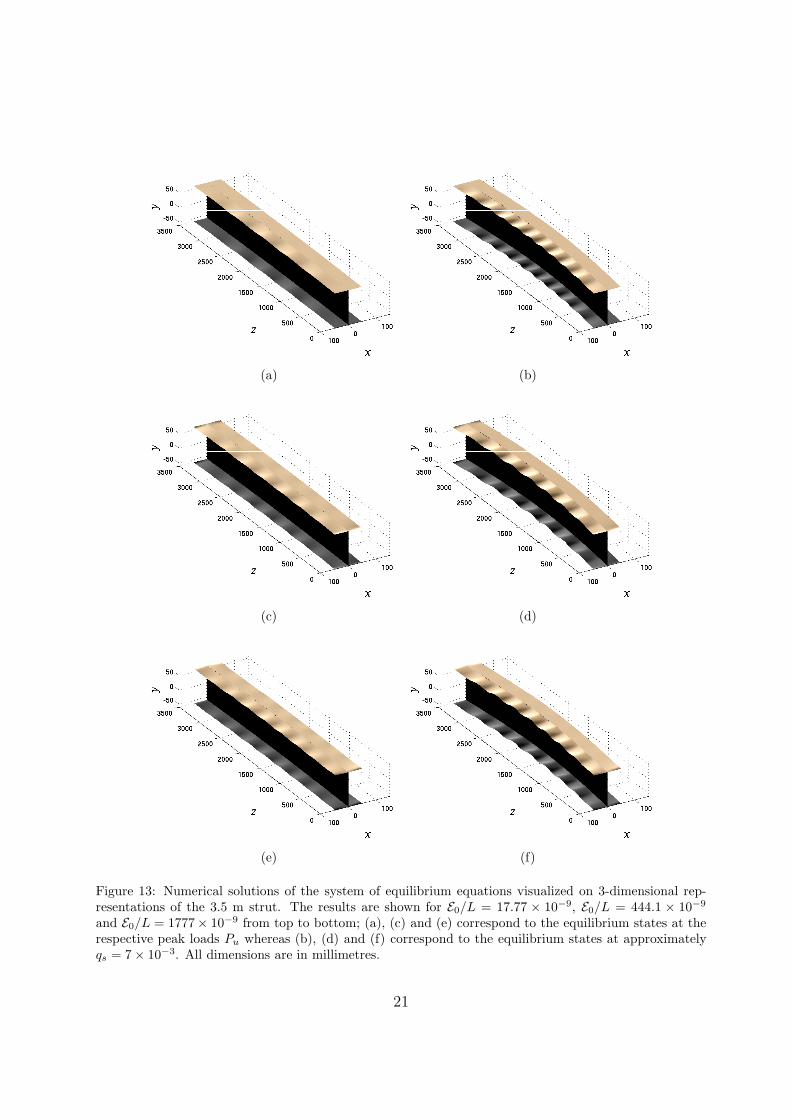
Figure 11(b) shows plots of equilibrium paths for the worst case modulated imperfec-tions, which correspond directly to Figure 11(a). As before, the cellular behaviour is af-fected by the initial shape of the imperfection. Figure 13 shows a selection of 3-dimensionalrepresentations of the deflected 3.5 m long strut that comprise all the components of globalbuckling (W and θ) and local buckling (wi and ui). The value of E0 increases from top tobottom; the left column corresponds to the equilibrium state at the peak load Pu whereasthe right column corresponds to the equilibrium state at a significantly larger magnitudeof the global mode, where qs = 7× 10⁻³, for each case of E0. It is clear that at peak loads,struts with larger imperfections have shorter local buckling wavelengths. Comparing thepair of struts with the smallest and the largest initial imperfection at qs = 7×10⁻³, it is ob-served that the strut with smaller E0 has developed approximately ten sinusoidal waves intotal along the length whereas the strut with larger E0 has a total number of eight sinusoidalwaves, which is the essentially same mode shape as its initial imperfection. No snap-backis observed on the equilibrium path in the latter case, implying there is no formation of anew peak or trough. However, as the buckling deformation increases, a snap-back may beexpected at a larger qs value, followed by a longer restabilization path until a total numberof 10 sinusoidal waves are fully formed. The corresponding equilibrium paths would thenbe expected to converge asymptotically.
3.4. Summary of findings
It is common practice to analyse the actual load-carrying capacity of structural com-pression members within a finite element framework by introducing perturbations in the
19
0 1000 2000 3000−0.2
0
0.2
w0 (
mm
)
z (mm)0 1000 2000 3000
−0.2
0
0.2
w0 (
mm
)
z (mm)
0 1000 2000 3000−0.2
0
0.2
w0 (
mm
)
z (mm)0 1000 2000 3000
−0.2
0
0.2
w0 (
mm
)z (mm)
0 1000 2000 3000−0.2
0
0.2
w0 (
mm
)
z (mm)0 1000 2000 3000
−0.2
0
0.2
w0 (
mm
)
z (mm)
0 1000 2000 3000−0.2
0
0.2
w0 (
mm
)
z (mm)0 1000 2000 3000
−0.2
0
0.2
w0 (
mm
)
z (mm)
0 1000 2000 3000−0.2
0
0.2
w0 (
mm
)
z (mm)0 1000 2000 3000
−0.2
0
0.2
w0 (
mm
)
z (mm)
0 1000 2000 3000−0.2
0
0.2
w0 (
mm
)
z (mm)0 1000 2000 3000
−0.2
0
0.2
w0 (
mm
)
z (mm)
Figure 12: Mode shapes of the initial out-of-plane displacement w0 showing the worst case combinationsof A0, β and α for the 3.5 m strut with increasing E0 values, shown in Figure 9, from top to bottom. Theleft column shows the worst case periodic imperfection (α = 0), whereas the right column shows the worstcase modulated imperfection. All dimensions are in millimetres.
20
(a) (b)
(c) (d)
(e) (f)
Figure 13: Numerical solutions of the system of equilibrium equations visualized on 3-dimensional rep-resentations of the 3.5 m strut. The results are shown for E0/L = 17.77 × 10⁻⁹, E0/L = 444.1 × 10⁻⁹
and E0/L = 1777× 10−9 from top to bottom; (a), (c) and (e) correspond to the equilibrium states at therespective peak loads Pu whereas (b), (d) and (f) correspond to the equilibrium states at approximatelyqs = 7 × 10⁻³. All dimensions are in millimetres.
21
form of an initial imperfection that are affine to linear eigenmodes [32]. In the vast majorityof cases, this is of course perfectly sensible since under increasing load the initial perturba-tion forces the component to deform into the minimum energy post-buckling configuration,which essentially matches the eigenvalue solution at least for moderately large deflections.However, as shown in the current study, in cases where there is significant mode interaction,the qualitative nature of the post-buckling profile can change very rapidly and may notresemble the linear eigenmode profile for moderately large deflections. Localization andsubsequent spreading of the buckling profile throughout the component with a changingwavelength makes it less obvious for analysts to know which perturbation profile to usefor calculating the load-carrying capacity. Hence, the worst case shape of the perturbationchanges qualitatively with increasing perturbation size and introducing imperfections thatare affine to eigenmodes may lead to unsafe predictions of the actual capacity.
It has been demonstrated in the current study that the imperfection that should beused is the one that matches the interactive post-buckling profile with the shape changingcorresponding to the size of the imperfection which is appropriate for the manufacturingtolerance [33]. Although it has been shown that a modulated imperfection invariably givesthe lowest peak load for a given imperfection size, the required degree of modulation isrelatively small and it seems to be far more important that the number of waves along thelength in the periodic component matches that of the actual post-buckling profile. Withcellular buckling occurring, the required number of waves along the length in the worstcase imperfection has been shown to increase with the imperfection size. Notwithstandingthe present findings, if the actual physically measured initial imperfection profile of thecomponent is available to the analyst then it should of course be used, but that wouldprobably be a rare occurrence within a design situation.
4. Concluding remarks
The nonlinear analytical model for the axially-loaded thin-walled I-section strut [4] hasbeen developed to include initial global and local imperfections. Studies investigating thesensitivity to the presence of global imperfections only, local imperfections only, and bothimperfection types in combination have been conducted. The highly sensitive nature of thestruts that are susceptible to cellular buckling to these different classes of initial imperfec-tion has been highlighted. Moreover, in the case of local flange imperfections, the shape ofthe worst case changes with the overall imperfection size. However, in contrast with earlierwork on sandwich struts [26], the current study shows that the wavelength of the initiallocal deflection affects the load-carrying capacity more significantly than the degree of lo-calization. When considering local flange imperfections it was found that the modulatedlocal imperfection always seems to be the worst case in terms of the load-carrying capacity,albeit by a narrow margin. Nevertheless, the study on different forms of global and localimperfections indicates the need for caution when designing such components; the commonpractice of determining actual load-carrying capacities by introducing imperfections thatare affine to the local buckling eigenmodes has been demonstrated not to predict the mostsevere responses in the presence of a strong local–global mode interaction.
22
It is worth recalling that the cross-section properties in all the numerical examples wereselected such that the global and the local critical loads were sufficiently close. These ge-ometries where the critical buckling loads are similar have been referred to in the literatureas lying in the ‘imperfection sensitive’ zone [1]. However, it is obvious that the individualglobal and local critical buckling loads would change with parametric variations in thestrut length, flange width, web height and the degree of joint rigidity between the web andthe flanges [5]. Different behaviours would then be expected in terms of imperfection sen-sitivity at both global and local slendernesses [18]. Therefore, further parametric analysesare vital for predicting the true load-carrying capacity of the structural component; thesestudies will be reported on soon.
References
[1] A. van der Neut, The interaction of local buckling and column failure of thin-walledcompression members, in: M. Hetenyi, W. G. Vincenti (Eds.), Proceedings of the 12thInternational Congress on Applied Mechanics, Springer, Berlin, 1969, pp. 389–399.
[2] J. M. T. Thompson, G. W. Hunt, A general theory of elastic stability, Wiley, London,1973.
[3] V. Gioncu, General theory of coupled instabilities, Thin-Walled Struct. 19 (2–4) (1994)81–127.
[4] M. A. Wadee, L. Bai, Cellular buckling in I-section struts, Thin-Walled Struct 81(2014) 89–100.
[5] L. Bai, M. A. Wadee, Mode interaction in thin-walled I-section struts with semi-rigidflange-web joints, International Journal of Non-Linear Mechanics 69 (2015) 71–83.
[6] G. J. Hancock, Interaction buckling in I-section columns, ASCE J. Struct. Eng 107 (1)(1981) 165–179.
[7] B. W. Schafer, Local, distortional, and Euler buckling of thin-walled columns, ASCEJ. Struct. Eng 128 (3) (2002) 289–299.
[8] D. Dubina, V. Ungureanu, Instability mode interaction: From Van Der Neut modelto ECBL approach, Thin-Walled Structures 81 (2014) 39–49.
[9] G. W. Hunt, L. S. da Silva, G. M. E. Manzocchi, Interactive buckling in sandwichstructures, Proc. R. Soc. A 417 (1988) 155–177.
[10] G. W. Hunt, M. A. Wadee, Localization and mode interaction in sandwich structures.,Proc. R. Soc. A 454 (1972) (1998) 1197–1216.
[11] M.-A. Douville, P. Le Grognec, Exact analytical solutions for the local and global buck-ling of sandwich beam-columns under various loadings, Int. J. Solids Struct. 50 (16–17)(2013) 2597–2609.
23
[12] W. T. Koiter, M. Pignataro, A general theory for the interaction between local andoverall buckling of stiffened panels, Tech. rept. WTHD 83, Delft University of Tech-nology, Delft, The Netherlands (1976).
[13] M. Pignataro, M. Pasca, P. Franchin, Post-buckling analysis of corrugated panels inthe presence of multiple interacting modes, Thin-Walled Struct. 36 (1) (2000) 47–66.
[14] K. G. Ghavami, M. R. Khedmati, Numerical and experimental investigation on thecompression behaviour of stiffened plates, J. Constr. Steel Res. 62 (11) (2006) 1087–1100.
[15] N. Olhoff, A. P. Seyrenian, Bifurcation and post-buckling analysis of bimodal optimumcolumns, Int. J. Solids Struct. 45 (14–15) (2008) 3967–3995.
[16] M. A. Wadee, M. Farsi, Cellular buckling in stiffened plates, Proc. R. Soc. A 470 (2168)(2014) 20140094.
[17] M. A. Wadee, M. Farsi, Local–global mode interaction in stringer-stiffened plates,Thin-Walled Struct. 85 (2014) 419–430.
[18] M. A. Wadee, M. Farsi, Imperfection sensitivity and geometric effects in stiffenedplates susceptible to cellular buckling, Structures 3 (2015) 172–186.
[19] M. A. Wadee, L. Gardner, Cellular buckling from mode interaction in I-beams underuniform bending, Proc. R. Soc. A 468 (2137) (2012) 245–268.
[20] G. W. Hunt, M. A. Peletier, A. R. Champneys, P. D. Woods, M. A. Wadee, C. J.Budd, G. J. Lord, Cellular buckling in long structures, Nonlinear Dyn 21 (1) (2000)3–29.
[21] J. Burke, E. Knobloch, Homoclinic snaking: Structure and stability, Chaos 17 (3)(2007) 037102.
[22] J. M. T. Thompson, G. H. M. van der Heijden, Quantified “shock-sensitivity” abovethe Maxwell load, Int. J. Bifurcation Chaos 24 (3) (2014) 1430009.
[23] J. Becque, K. J. R. Rasmussen, Experimental investigation of the interaction of localand overall buckling of stainless steel I-columns, ASCE J. Struct. Eng. 135 (11) (2009)1340–1348.
[24] J. Becque, K. J. R. Rasmussen, Numerical investigation of the interaction of local andoverall buckling of stainless steel I-columns, ASCE J. Struct. Eng. 135 (11) (2009)1349–1356.
[25] A. van der Neut, The sensitivity of thin-walled compression members to column axisimperfection, Int. J. Solids Struct. 9 (1973) 999–1011.
24
[26] M. A. Wadee, Effects of periodic and localized imperfections on struts on nonlinearfoundations and compression sandwich panels, Int. J. Solids Struct. 37 (8) (2000)1191–1209.
[27] E. J. Doedel, B. E. Oldeman, Auto-07p: Continuation and bifurca-tion software for ordinary differential equations, Tech. rep., Department ofComputer Science, Concordia University, Montreal, Canada, available fromhttp://indy.cs.concordia.ca/auto/ (2009).
[28] P. S. Bulson, The stability of flat plates, Chatto & Windus, London, UK, 1970.
[29] M. K. Wadee, G. W. Hunt, A. I. M. Whiting, Asymptotic and Rayleigh–Ritz routesto localized buckling solutions in an elastic instability problem, Proc. R. Soc. A453 (1965) (1997) 2085–2107.
[30] J. M. T. Thompson, G. W. Hunt, Elastic instability phenomena, Wiley, London, 1984.
[31] S. P. Timoshenko, J. M. Gere, Theory of elastic stability, McGraw-Hill, New York,USA, 1961.
[32] T. Belytschko, W. K. Liu, B. Moran, Nonlinear finite elements for continua and struc-tures, Wiley, Chichester, 2000.
[33] EN1993-1-1, Eurocode 3: Design of steel structures - Part 1-1: General rules and rulesfor buildings, British Standards Institution, 2005.
25