Impacts of various boundary conditions on beam vibrations

Graduate Theses, Dissertations, and Problem Reports

2015

Impacts of various boundary conditions on beam vibrations Impacts of various boundary conditions on beam vibrations

Ye Tao

Follow this and additional works at: https://researchrepository.wvu.edu/etd

Recommended Citation Recommended Citation Tao, Ye, "Impacts of various boundary conditions on beam vibrations" (2015). Graduate Theses, Dissertations, and Problem Reports. 6774. https://researchrepository.wvu.edu/etd/6774

This Thesis is protected by copyright and/or related rights. It has been brought to you by the The Research Repository @ WVU with permission from the rights-holder(s). You are free to use this Thesis in any way that is permitted by the copyright and related rights legislation that applies to your use. For other uses you must obtain permission from the rights-holder(s) directly, unless additional rights are indicated by a Creative Commons license in the record and/ or on the work itself. This Thesis has been accepted for inclusion in WVU Graduate Theses, Dissertations, and Problem Reports collection by an authorized administrator of The Research Repository @ WVU. For more information, please contact [email protected].

https://researchrepository.wvu.edu/

https://researchrepository.wvu.edu/

https://researchrepository.wvu.edu/etd

https://researchrepository.wvu.edu/etd?utm_source=researchrepository.wvu.edu%2Fetd%2F6774&utm_medium=PDF&utm_campaign=PDFCoverPages

https://researchrepository.wvu.edu/etd/6774?utm_source=researchrepository.wvu.edu%2Fetd%2F6774&utm_medium=PDF&utm_campaign=PDFCoverPages

mailto:[email protected]

IMPACTS OF VARIOUS BOUNDARY CONDITIONS ON

BEAM VIBRATIONS

Ye Tao

Thesis submitted to the

Benjamin M. Statler College of Engineering and Mineral Resources

at West Virginia University

in partial fulfillment of the requirements for the degree of

Master of Science

in

Civil Engineering

Roger H. L. Chen, Ph.D., Chair

Omar Abdul-Aziz, Ph.D.

Horng-Jyh Yang, Ph.D.

Marvin Cheng., Ph.D.

Department of Civil Engineering and Environmental Engineering

Morgantown, West Virginia 2015

Keywords: Euler-Bernoulli Beam, Timoshenko Beam, Various Boundary

Conditions, Free Vibrations, Forced Vibrations, Spring Constraints.

ABSTRACT

Impacts of Various Boundary Conditions on Beam Vibrations

Ye Tao

In real life, boundary conditions of most structural members are neither totally fixed nor

completely free. It is crucial to study the effect of boundary conditions on beam vibrations. This

thesis focuses on deriving analytical solutions to natural frequencies and mode shapes for

Euler-Bernoulli Beams and Timoshenko Beams with various boundary conditions under free

vibrations. In addition, Green’s function method is employed to solve the close-form expression

of deflection curves for forced vibrations of Euler-Bernoulli Beams and Timoshenko Beams.

A direct and general beam model is set up with two different vertical spring constraints

𝑘𝑇1, 𝑘𝑇2 and two different rotational spring constraints 𝑘𝑅1, 𝑘𝑅2 attached at the ends of the beam.

These end constraints can represent various combinations of boundary conditions of the beam by

varying the spring constraints. A general solution for the Timoshenko beam with this various

boundary conditions is derived, and to the best of our knowledge, this solution is not available in

the literature. Numerical examples are presented to illustrate the effects of the end constraints on

the natural frequencies and mode shapes between Euler-Bernoulli beams and Timoshenko beam.

The results show that Euler-Bernoulli beams have higher natural frequencies than Timoshenko

beams at different modes. The ratio of the natural frequencies for Timoshenko beams to the

natural frequency for Euler-Bernoulli beams decreases at higher modes. Natural frequencies at

lower modes are more sensitive to boundary constraints than natural frequencies at higher

modes.

iii

ACKNOWLEGEMENTS

I would like to express my gratitude and appreciation to everyone who helped to make this

thesis possible.

First of all, I would like to recognize my advisor Dr. Roger Chen for his superb guidance,

incredible knowledge, proficient editing skills, and great support throughout my study at West

Virginia University.

Second, I would like to thank my labmates Mr. Yun Lin, Mr. Zhanxiao Ma, and Mr. Alper

Yikici for their assistance and suggestions during my project.

My thanks also go to other three committee members, Dr. Omar Abdul-Aziz, Dr. Hong-

Jyh Yang, and Dr. Marvin Cheng for their advice, feedback, and direction. I would like to extend

my appreciation to all the faculty and staff in the Department of Civil and Environmental

Engineering at WVU.

Finally, I would like to thank my parents, Mrs. Hong Chen and Mr. Shijun Tao for their

unconditioned love, constant encouragement, and extraordinary patience. I also feel blessed to

have Di Wang accompany me in my life.

iv

TABLE OF CONTENTS

LIST OF FIGURES ............................................................................................................................... vi

LIST OF TABLES ................................................................................................................................ vii

NOMENCLATURE ............................................................................................................................ viii

CHAPTER 1 Introduction ..................................................................................................................... 1

1.1 Introduction ................................................................................................................................ 1

1.2 Objectives ................................................................................................................................... 2

CHAPTER 2 Literature Review ........................................................................................................... 3

2.1 Previous Studies ......................................................................................................................... 3

2.2 Euler-Bernoulli Theory .............................................................................................................. 5

2.3 Timoshenko Beams Theory ........................................................................................................ 6

2.4 Green’s Function ........................................................................................................................ 7

Chapter 3 Free Vibrations of Euler-Bernoulli Beams ........................................................................ 9

3.1 Natural Frequencies and Mode Shapes of an Euler-Bernoulli Beam with various boundary

conditions .................................................................................................................................... 9

3.2 Natural Frequencies and Mode Shapes of a Cantilever Euler-Bernoulli Beam with a Rotational

Spring and a Vertical Spring ..................................................................................................... 13

3.3 Natural Frequencies and Mode Shapes of an Euler-Bernoulli Beam with Two Rotational

Springs and Two Fixed Vertical Supports ................................................................................ 15

Chapter 4 Free Vibration of Timoshenko Beams .............................................................................. 18

4.1 Timoshenko Beams under Free Vibrations .............................................................................. 18

4.2 Natural Frequencies and Mode Shapes of a Timoshenko Beam with Various Boundary

Conditions ................................................................................................................................. 22

4.3 Natural Frequencies and Mode Shapes of a Cantilever Timoshenko Beam with a Rotational

Spring and a Vertical Spring ..................................................................................................... 27

4.4 Natural Frequencies and Mode Shapes of a Timoshenko Beam with Two Rotational Springs

and Two Fixed Vertical Supports ............................................................................................. 30

CHAPTER 5 Forced Vibrations of Euler-Bernoulli Beams ............................................................. 34

5.1 Deflection Curves of Forced Vibrations of Euler-Bernoulli Beams ........................................ 34

5.2 Forced Vibrations of Euler-Bernoulli Beams with Two Different Rotational Springs and Two

Different Vertical Springs ......................................................................................................... 37

5.3 Forced Vibration of Simply Supported Euler-Bernoulli Beams .............................................. 40

v

CHAPTER 6 Forced Vibrations of Timoshenko Beams ................................................................... 42

6.1 Deflection Curves of Forced Vibrations of Timoshenko Beams ............................................. 42

6.2 Forced Vibrations of Timoshenko Beams with Two Different Rotational Springs and Two

Different Vertical Springs ......................................................................................................... 48

6.3 Forced Vibrations of Simply Supported Timoshenko Beams .................................................. 50

CHAPTER 7 Results and Discussion .................................................................................................. 52

7.1 Comparison of Natural Frequencies between Euler-Bernoulli Beams and Timoshenko Beams

under Free Vibrations ............................................................................................................... 52

7.2 Comparison of Mode Shapes between Euler-Bernoulli Beams and Timoshenko Beams under

Free Vibrations.......................................................................................................................... 56

7.2.1 Mode shapes Comparison of a Cantilever Beam under Free Vibration.......................... 56

7.2.2 Comparison of Mode Shapes of a Beam with Two Fixed Vertical Supports and Two

Rotational Springs under Free Vibrations ...................................................................... 61

7.3 Deflection Curves Comparison of Forced Vibrations .............................................................. 65

7.3.1 Deflection Curves of a Simply Supported Beam under Forced Vibrations .................... 65

7.3.2 Deflection Curves of a Beam with Two Fixed Vertical Supports and Two Rotational

Springs under Forced Vibrations .................................................................................... 68

Chapter 8 Conclusions and Recommendations ................................................................................. 72

8.1 Conclusions .............................................................................................................................. 72

8.2 Recommendations .................................................................................................................... 73

References ............................................................................................................................................. 74

Appendixes ............................................................................................................................................ 77

Appendix I Dimensionless Frequencies of Euler-Bernoulli Beams ............................................... 77

Appendix II Dimensionless Frequencies of Timoshenko Beams ................................................... 78

Appendix III First Five Mode shapes for Euler-Bernoulli Beams ................................................. 79

Appendix IV First Five Mode shapes for Timoshenko Beams ...................................................... 83

Vita……………………………………………………………………………………………………..88

vi

LIST OF FIGURES

Figure 3.1: An Euler-Bernoulli Beam with Two Rotational Springs and Two Vertical Spring

................................................................................................ …………………….9

Figure 3.2: A cantilever Euler-Bernoulli Beam ....................................................................... 14

Figure 3.3: An Euler-Bernoulli Beam with Two Rotational Springs ...................................... 15

Figure 3.4: A Simply Supported Euler-Bernoulli Beam .......................................................... 17

Figure 4.1: Sign Conventions for Timoshenko Beams ............................................................ 18

Figure 4.2: A Timoshenko Beam with Two Rotational Springs and Two Vertical Springs ... 23

Figure 4.3: A Cantilever Timoshenko Beam with a Rotational Spring and a Vertical Spring 27

Figure 4.4: A Timoshenko Bernoulli Beam with Two Rotational Springs ............................. 30

Figure 7.1: A Cantilever Beam with a Rotational Spring ........................................................ 52

Figure 7.2: Frequency Ratio (fT/fEB) between Timoshenko Beam and Euler-Bernoulli Beam

Due to Different k^, and Dimensionless Inverse Ratio r ...................................... 55

Figure 7.3: First Five Mode Shapes for a Cantilever Euler-Bernoulli beam ........................... 57

Figure 7.4: First Five Mode Shapes of a Cantilever Timoshenko Beam ................................. 58

Figure 7.5: Comparison of Superimposed Mode Shapes for a Cantilever Beam .................... 59

Figure 7.6(a): Huang’s Results Superimposed Mode Shapes for a Cantilever Beam (Dashed Line:

Euler-Bernoulli Beam, Continuous Line: Timoshenko Beam)…………………..60

Figure 7.6(b): Superimposed Mode Shapes for a Cantilever Beam from This Thesis (Dashed Line:

Euler-Bernoulli Beam, Continuous Line: Timoshenko Beam)…………………..60

Figure 7.7: A Beam with Two Different Rotational Springs……...………………………….61

Figure 7.8: First Five Modes Shapes for an Euler-Bernoulli Beam with Two Different

Rotational Springs ................................................................................................. 62

Figure 7.9: First Five Modes Shapes for a Timoshenko beam with Two Different Rotational

Springs .................................................................................................................. 63

Figure 7.10: Comparison of Superimposed Mode Shapes for a Beam with Two Different

Rotational Springs ................................................................................................. 64

Figure 7.11: Comparison of Deflection Curves of a Simply Supported Beam under Forced

Vibrations .............................................................................................................. 67

Figure 7.12: Lueschen's plots for Comparison of Deflection Curves of a Simply Supported

Beam under Forced Vibrations ............................................................................. 68

Figure 7.13: Comparison of Deflection Curves of a Beam with Two Rotational Springs under

Forced Vibrations.................................................................................................. 70

vii

LIST OF TABLES

Table 7.1: Beam Properties for the Numerical Example in Section 7.1 .................................... 52

Table 7.2: Comparison of Frequency Ratio (fT/fEB) between Timoshenko Beam and Euler-

Bernoulli Beam with Various Boundary Conditions ................................................ 53

Table 7.3: Chen and Kiriakidis's Results for Comparison of Frequency Ratio (fT/fEB) between

Timoshenko Beam and Euler-Bernoulli Beam with Various Boundary

Conditions..................................................................................................................53

Table 7.4: Beam Properties for the Numerical Example in 7.1.2 .............................................. 56

Table 7.5: Beam Properties for the Numerical Example in 7.3.1 .............................................. 65

viii

NOMENCLATURE

The following symbols are used in the thesis:

A = cross section area

E = Young’s Modulus

G = modulus of rigidity

I = moment of inertia

k = dimensionless frequency of Euler-Bernoulli beams

K = numerical shape factor

𝑘𝑅1 = rotational spring constant on left hand side of the beam

𝑘𝑅2 = rotational spring constant on right hand side of the beam

𝑘𝑇1 = vertical spring constant on left hand side of the beam

𝑘𝑇2 = vertical spring constant on right hand side of the beam

k^ = rotational spring constant = 𝑘𝑅1𝐿

𝐸𝐼

L = beam length

M = bending moment

q = external load

t = time

V = shear force

Y = transverse deflection of the free vibration

𝜉 = dimensionless length = 𝑥/𝐿

𝜉𝑓 = the point where the point load is applied at

Ψ = bending slope

𝜌 = density

ω = angular natural frequency of beam vibrations

𝜔𝜔 = angular frequency of the applied load

ʋ = Poisson ratio

𝑏2 = dimensionless frequency for Timoshenko beams = 𝜌𝐴𝐿4𝜔2 / (𝐸𝐼)

𝑟2 = 𝐼/(𝐴𝐿2)

𝑠2 = 𝐸𝐼/(𝐾𝐴𝐺𝐿2)

𝛼 = √1

2[−(𝑟2 + 𝑠2) + √(𝑟2 − 𝑠2)2 +

4

𝑏2 ]

𝛽 = √1

2[(𝑟2 + 𝑠2) + √(𝑟2 − 𝑠2)2 +

4

𝑏2 ]

ix

𝛾4 = 𝜌𝐴𝐿4𝜔2

𝐸𝐼

fT/fEB = Natural frequency ratio of the Timoshenko beam to the Euler-Bernoulli beam

µ = √1

2[(𝑟2 + 𝑠2) − √(𝑟2 − 𝑠2)2 +

4

𝑏2 ]

1

CHAPTER 1 Introduction

1.1 Introduction

Beam vibration is an important and interesting topic. Structures subjected to

random vibrations can cause fatigue failures. When a beam is excited by a steady-state

harmonic load, it vibrates at the same frequency as the frequency of the applied

harmonic load. When the applied loading frequency equals to one of the natural

frequencies of the system, large oscillation occurs, which can cause large beam

deflection. This phenomenon is called resonance. Therefore, determination of natural

frequencies is crucial in vibration problems.

Continuous structural beam systems are widely used in many engineering fields,

such as structural engineering, transportation engineering, mechanical engineering, and

aerospace engineering. The boundary conditions of structural members in continuous

structural beam systems are indeterminate and complicated. It is not accurate to assume

these boundary conditions as totally fixed or completely free.

In this thesis, a direct and general beam model is set up with two different

rotational springs and two different vertical springs at both ends to simulate different

beam boundary conditions. Dynamic responses of Euler-Bernoulli beams and

Timoshenko beams under free vibrations and forced vibrations are analyzed. Euler-

Bernoulli beam theory is also known as the classical beam theory. It is a simplification

of the linear theory of elasticity which presents the relationship between the applied

2

load and the deflection of a slender beam. However the classical one-dimensional

Euler-Bernoulli theory is not accurate enough for deep beams and the vibrations at

higher modes. Timoshenko Beam theory counts in the effects of rotatory inertia and

transverse-shear deformation, which are introduced by Rayleigh in 1842 and by

Timoshenko in 1921, respectively. To the best of our knowledge, no one has derived

the general solution for the Timoshenko beam vibration with arbitrary beam boundary

conditions yet.

1.2 Objectives

The objectives of this thesis are: First, derive the solutions to the natural

frequencies and the mode shapes of Euler-Bernoulli beams and Timoshenko beams

with various boundary conditions under free vibration using eigenvalues and

eigenvectors. Second, obtain the close-form expression of deflection shapes of Euler-

Bernoulli beams and Timoshenko beams under forced vibrations using Green’s

function. Last, compare the effects of various boundary conditions on vibrations of

Euler-Bernoulli beams and Timoshenko beams.

3

CHAPTER 2 Literature Review

2.1 Previous Studies

Vibrations of Euler-Bernoulli beams and Timoshenko beams have been studied

by many researchers over the past decades. Huang (1961) presented normal modes and

natural frequency equations of six types of Timoshenko beams with different end

constraints under free vibrations: supported-supported beam, free-free beam, clamped-

clamped beam, clamped-free beam, clamped-supported beam, and supported-free beam.

Ross and Wang (1985) derived the frequency equation for a Timoshenko beam with

two identical spring constraints 𝑘𝑅 and two fixed vertical supports. Chen and

Kiriakidis (2005) derived the frequency equation for the cantilever Timoshenko beam

with a rotational spring and a vertical spring. Majkut (2009) analyzed the Timoshenko

beam with identical vertical spring constraints 𝑘𝑇 , and identical rotational spring

constraints 𝑘𝑅 at both ends. But he made a mistake on the equation of moments acting

on infinitesimal beam element. The moment should be caused by pure bending angle,

instead of the sum of bending angle and shear angle.

Different approaches have been employed to solve forced vibrations of Euler-

Bernoulli beams and Timoshenko beams, such as the mode superposition method, and

the dynamic Green’s function method. Mode superposition method is an approximate

method since truncations are used in the computation of the finite series. Hamada (1981)

solved the solution for a simply supported and damped Euler-Bernoulli beam under a

4

moving load using double Laplace transform. Mackertich (1992) studied beam

deflections of a simple supported Euler-Bernoulli beam and a simple supported

Timoshenko beam using mode superposition method. Esmailzadeh and Ghorashi (1997)

analyzed the dynamic response of a simply supported Timoshenko beam excited by

uniformly distributed moving masses using finite difference method. Ekwaro-Osire et

al. (2001) solved the deflection curve for a hinged-hinged Timoshenko beam by series

expansion method. Uzzal et al. (2012) studied the vibrations of an Euler-Bernoulli beam

supported on Pasternak foundation under a moving load by Fourier transform and mode

superposition method. Azam et al. (2013) presented the dynamic response of a

Timoshenko beam excited by a moving sprung mass using mode superposition method.

Roshandel et al. (2015) investigated the dynamic response of a Timoshenko beam

excited by a moving mass using Eigenfunction expansion method.

Green’s function method is more straightforward and efficient compared to

mode superposition method. There is no need to calculate natural frequencies and mode

shapes for the beam for Green’s function method. Many people have contributed to

finding the corresponding Green’s functions for beam vibrations. Mohamad (1994)

tabulated the solutions for mode shapes of Euler-Bernoulli beams with intermediate

attachments using Green’s function. Lueschen (1996) derived the corresponding

Green’s function for forced Timoshenko beams vibrations in frequency domain using

Laplace Transform for the same six beam types of as Huang’s (1961). Foda and

Abduljabbar (1997) studied the dynamic response of a simply supported Euler-

Bernoulli beam under a moving mass using Green’s function. Abu-Hilal (2003)

5

investigated the dynamic response of a cantilever Euler-Bernoulli beam with elastic

support under distributed and concentrated loads using Green’s function. Mehri et al.

(2009) studied the forced vibrations of an Euler-Bernoulli beam with two identical

rotational springs and two identical verticals springs under a moving load. Li and Zhao

(2014) derived the steady-state Green’s functions for deflection curve of forced

vibrations of Timoshenko beam with a harmonic force considering damping effects for

six types of beams for the same six beam types of as Huang’s (1961).

However, to the best of our knowledge, the general solution to dynamic

responses of a Timoshenko beam that can be applied to any arbitrary boundary

conditions is not available in the literature yet.

2.2 Euler-Bernoulli Theory

Euler-Bernoulli theory is applied to a beam with one dimension much larger

than the other two dimensions. There are three assumptions for the Euler-Bernoulli

beam theory: First, the cross section is assumed to be elastic isotropic with small

deflection. Second, the cross section of the beam remains plane after bending. Third,

the cross section remains normal to the deformed axis of the beam.

The classical beam theory describes the relationship between the deflection of

the beam, y(x, t) and the bending moment, 𝑀(𝑥, 𝑡):

𝑀(𝑥, 𝑡) = 𝐸𝐼𝜕2𝑦

𝜕𝑥2 (2.1)

6

y represents the transverse displacement of an element of the beam. x stands for

the distance from the left hand end. E denotes the Young’s modulus. I(x) is the moment

of inertia of the section.

From Timoshenko’s (1990) book Vibration Problems in Engineering, the mode

shape for the Euler-Bernoulli beam under free vibration can be stated as:

𝑦(𝑥, 𝑡) = 𝑌(𝑥)𝑇(𝑡) (2.2a)

𝑌(𝑥) = 𝐶1𝑠𝑖𝑛(𝑘𝑥) + 𝐶2𝑐𝑜𝑠(𝑘𝑥) + 𝐶3𝑠𝑖𝑛ℎ(𝑘𝑥) + 𝐶4𝑐𝑜𝑠ℎ(𝑘𝑥) (2.2b)

𝑇(𝑡) = 𝐴𝑐𝑜𝑠(𝜔𝑡) + 𝐵𝑠𝑖𝑛(𝜔𝑡) (2.2c)

k denotes the dimensionless frequency of the beam. 𝜔 denotes the angular

frequency. 𝐶1 to 𝐶4 can be determined by the boundary conditions.

k and 𝜔 can be related to each other by:

ωi = (ki)2√

EI

ρA (i = 1, 2, 3, 4, 5 …… . , ∞) (2.3)

2.3 Timoshenko Beams Theory

Stephen Timoshenko introduced Timoshenko Beam theory in early 20th century

(Timoshenko, 1921). The Timoshenko Beam theory takes effects of rotary inertia and

shear deformations into account. It is suitable for describing the behavior of short beams,

beams vibrating at high frequency modes. The extra mechanism of deformation reduces

the stiffness of the beam, causing larger deflection and lower Eigen frequencies. The

7

governing equations of Timoshenko beams are 4𝑡ℎorder partial differential equations.

The governing equations for Timoshenko Beams are shown as

𝐸𝐼𝜕2𝜑

𝜕𝑥2+ 𝐾𝐴𝐺 (

𝜕𝑦

𝜕𝑥− 𝜑) − 𝜌𝐼

𝜕2𝜑

𝜕𝑡2= 0 (2.4a)

−𝜌𝐴𝜕2𝑦

𝜕𝑡2 + 𝐾𝐴𝐺 (𝜕2𝑦

𝜕𝑥2 −𝜕𝜑

𝜕𝑥) = 0 (2.4b)

G, denotes modulus of rigidity; A, denotes cross section area; K, denotes

numerical shape factor; y, denotes transverse deflection; 𝜑 denotes bending slope.

2.4 Green’s Function

The concept of Green’s function is developed by George Green in 1830s

(Challis and Sheard 2003). Green’s function is defined as the impulse response of a

nonhomogeneous differential equation in a bounded region. It can be used to solve the

solution to nonhomogeneous boundary value problems. It provides a visual

interpretation of the response of a system with a unit point source.

Define a linear differential operator L, acting on distributions over a subset of

𝑅𝑛 Euclidean space. At a point 𝑥𝑓 , a Green’s function G(x,𝑥𝑓 ) has the following

property:

L{𝐺(𝑥, 𝑥𝑓)} = 𝛿 (𝑥 − 𝑥𝑓) (2.5)

δ is the Dirac delta function. The definition for Dirac delta function is:

𝛿 (𝑥) = {+∞ 𝑥 = 0

0 𝑥 ≠ 0 (2.6)

8

The Dirac delta function has an important property that

∫ 𝑓(𝑥)𝛿 (𝑥 − 𝑎) 𝑑𝑥 = 𝑓(𝑎)∞

−∞ (2.7)

9

Chapter 3 Free Vibrations of Euler-Bernoulli Beams

3.1 Natural Frequencies and Mode Shapes of an Euler-Bernoulli Beam with various

boundary conditions

In real world, boundary conditions of a beam are complicated. In most cases, it is neither

perfectly fixed, nor completely free. In this section, a general model of an Euler-Bernoulli beam

is studied, which is a beam with two different rotational springs and two different vertical

springs at the ends. It is demonstrated below:

Figure 3.1: An Euler-Bernoulli Beam with Two Rotational Springs and Two Vertical

Springs

𝑘𝑅1 and 𝑘𝑇1 represent the rotational spring constant and the vertical spring on the left

hand side of the beam, respectively. 𝑘𝑅2 and 𝑘𝑇2 represent the rotational spring constant and

the vertical spring on the right hand side of the beam, respectively. By varying the spring

constants of the two rotational springs and two vertical springs, various beam boundary

conditions can be simulated.

The transverse vibration mode shape can be written as:

𝑌(𝜉) = 𝐶1𝑠𝑖𝑛(𝑘𝜉) + 𝐶2𝑐𝑜𝑠(𝑘𝜉) + 𝐶3𝑠𝑖𝑛ℎ(𝑘𝜉) + 𝐶4𝑐𝑜𝑠ℎ(𝑘𝜉) (3.1)

10

where 𝜉 is the dimensionless length x/L.

The boundary conditions are shown below:

𝑀⃒𝜉=0 = 𝑘𝑅1𝛹⃒𝜉=0 , 𝑀⃒𝜉=1 = −𝑘𝑅2𝛹⃒𝜉=1

𝑉⃒𝜉=0 = −𝑘𝑇1𝑌⃒𝜉=0, 𝑉⃒𝜉=1 = 𝑘𝑇2𝑌⃒𝜉=1 (3.2)

Sign conventions for positive moment and positive shear are defined as:

+M +V

The bending moment M, bending slope 𝛹, and shear force V can be calculated by:

𝑀(𝜉) =𝐸𝐼𝑘2

𝐿2 [−𝐶1𝑠𝑖𝑛(𝑘𝜉) − 𝐶2𝑐𝑜𝑠(𝑘𝜉) + 𝐶3𝑠𝑖𝑛ℎ(𝑘𝜉) + 𝐶4𝑐𝑜𝑠ℎ(𝑘𝜉)]

𝛹(𝜉) =𝑘

𝐿[𝐶1𝑐𝑜𝑠(𝑘𝜉) − 𝐶2𝑠𝑖𝑛(𝑘𝜉) + 𝐶3𝑐𝑜𝑠ℎ(𝑘𝜉) + 𝐶4𝑠𝑖𝑛ℎ(𝑘𝜉)]

Figure 3.2: Sign Convention

11

𝑉(𝜉) =𝐸𝐼𝑘3

𝐿3[−𝐶1𝑐𝑜𝑠(𝑘𝜉) + 𝐶2𝑠𝑖𝑛(𝑘𝜉) + 𝐶3𝑐𝑜𝑠ℎ(𝑘𝜉) + 𝐶4𝑠𝑖𝑛ℎ(𝑘𝜉)] (3.3)

The boundary conditions can be rewritten in matrix format as:

[ 𝑘𝑅1

𝑘𝐸𝐼

𝐿𝑘𝑅1 −

𝑘𝐸𝐼

𝐿

−𝐸𝐼𝑘3

𝐿3 𝑘𝑇1

𝐸𝐼𝑘3

𝐿3 𝑘𝑇1

−𝐸𝐼𝑘2

𝐿2𝑠𝑖𝑛(𝑘) +

𝑘

𝐿𝑘𝑅2𝑐𝑜𝑠(𝑘) −

𝐸𝐼𝑘2

𝐿2𝑐𝑜𝑠(𝑘) −

𝑘

𝐿𝑘𝑅2𝑠𝑖𝑛(𝑘)

𝐸𝐼𝑘2

𝐿2𝑠𝑖𝑛ℎ(𝑘) +

𝑘

𝐿𝑘𝑅2𝑐𝑜𝑠ℎ(𝑘)

𝐸𝐼𝑘2

𝐿2𝑐𝑜𝑠ℎ (𝑘) +

𝑘

𝐿𝑘𝑅2𝑠𝑖𝑛ℎ(𝑘)

−𝐸𝐼𝑘3

𝐿3𝑐𝑜𝑠(𝑘) − 𝑘𝑇2𝑠𝑖𝑛(𝑘)

𝐸𝐼𝑘3

𝐿3𝑠𝑖𝑛(𝑘) − 𝑘𝑇2𝑐𝑜𝑠(𝑘)

𝐸𝐼𝑘3

𝐿3𝑐𝑜𝑠ℎ(𝑘) − 𝑘𝑇2𝑠𝑖𝑛ℎ(𝑘)

𝐸𝐼𝑘3

𝐿3𝑠𝑖𝑛ℎ(𝑘) − 𝑘𝑇2𝑐𝑜𝑠ℎ(𝑘) ]

×

[ 𝐶1

𝐶2

𝐶3

𝐶4]

=

[ 0

0

0

0]

(3.4)

To find the nontrivial solution of 𝐶1 to 𝐶4, determinant of the four by four matrix must equal to zero. The frequency equation can be

written as:

12

[−𝐸𝐼𝑘2

𝐿2𝑠𝑖𝑛(𝑘) +

𝑘

𝐿𝑘𝑅2𝑐𝑜𝑠(𝑘)] × [

𝑘𝐸𝐼

𝐿×

𝐸𝐼𝑘3

𝐿3× (

𝐸𝐼𝑘3

𝐿3𝑠𝑖𝑛ℎ(𝑘) − 𝑘𝑇2𝑐𝑜𝑠ℎ(𝑘)) + 𝑘𝑅1 × 𝑘𝑇1 × (

𝐸𝐼𝑘3

𝐿3𝑠𝑖𝑛(𝑘) − 𝑘𝑇2𝑐𝑜𝑠(𝑘)) −

𝑘𝐸𝐼

𝐿×

𝑘𝑇1 × ( 𝐸𝐼𝑘3

𝐿3 𝑐𝑜𝑠ℎ(𝑘) − 𝑘𝑇2𝑠𝑖𝑛ℎ(𝑘) ) +𝑘𝐸𝐼

𝐿×

𝐸𝐼𝑘3

𝐿3 × (𝐸𝐼𝑘3

𝐿3 𝑠𝑖𝑛(𝑘) − 𝑘𝑇2𝑐𝑜𝑠(𝑘)) −𝑘𝐸𝐼

𝐿× 𝑘𝑇1 (

𝐸𝐼𝑘3

𝐿3 𝑐𝑜𝑠ℎ(𝑘) − 𝑘𝑇2 𝑠𝑖𝑛ℎ(𝑘)) − 𝑘𝑇1 × 𝑘𝑅1 ×

( 𝐸𝐼𝑘3

𝐿3𝑠𝑖𝑛ℎ(𝑘) − 𝑘𝑇2𝑐𝑜𝑠ℎ(𝑘)) + [

𝐸𝐼𝑘2

𝐿2𝑐𝑜𝑠(𝑘) +

𝑘

𝐿𝑘𝑅2𝑠𝑖𝑛(𝑘)] × [𝑘𝑅1 ×

𝐸𝐼𝑘3

𝐿3(

𝐸𝐼𝑘3

𝐿3𝑠𝑖𝑛ℎ(𝑘) − 𝑘𝑇2𝑐𝑜𝑠ℎ(𝑘)) + 𝑘𝑇1 × 𝑘𝑅1 × (−

𝐸𝐼𝑘3


𝑘𝑇2𝑠𝑖𝑛(𝑘)) +𝑘𝐸𝐼

𝐿×

𝐸𝐼𝑘3


𝐿3 𝑐𝑜𝑠ℎ(𝑘) − 𝑘𝑇2𝑠𝑖𝑛ℎ(𝑘)) +𝑘𝐸𝐼

𝐿×

𝐸𝐼𝑘3

𝐿3 × (−𝐸𝐼𝑘3

𝐿3 𝑐𝑜𝑠(𝑘) − 𝑘𝑇2𝑠𝑖𝑛(𝑘)) − 𝑘𝑇1 × 𝑘𝑅1 × (𝐸𝐼𝑘3

𝐿3 𝑐𝑜𝑠ℎ(𝑘) −

𝑘𝑇2𝑠𝑖𝑛ℎ(𝑘)) + 𝑘𝑅1 ×𝐸𝐼𝑘3

𝐿3× (

𝐸𝐼𝑘3

𝐿3𝑠𝑖𝑛ℎ(𝑘) − 𝑘𝑇2𝑐𝑜𝑠ℎ(𝑘))] + [

𝐸𝐼𝑘2

𝐿2× 𝑠𝑖𝑛ℎ(𝑘) +

𝑘

𝐿× 𝑘𝑅2 × 𝑐𝑜𝑠ℎ(𝑘)] × [ 𝑘𝑇1 × 𝑘𝑅1 × (

𝐸𝐼𝑘3

𝐿3𝑠𝑖𝑛ℎ(𝑘) −

𝑘𝑇2𝑐𝑜𝑠ℎ(𝑘)) +𝑘𝐸𝐼

𝐿× 𝑘𝑇1 (−

𝐸𝐼𝑘3

𝐿3𝑐𝑜𝑠(𝑘) − 𝑘𝑇2𝑠𝑖𝑛(𝑘)) +

𝑘𝐸𝐼

𝐿×

𝐸𝐼𝑘3

𝐿3× (

𝐸𝐼𝑘3

𝐿3𝑠𝑖𝑛(𝑘) − 𝑘𝑇2𝑐𝑜𝑠(𝑘)) +

𝑘𝐸𝐼

𝐿× 𝑘𝑇1 (−

𝐸𝐼𝑘3


𝑘𝑇2𝑠𝑖𝑛(𝑘)) − 𝑘𝑇1 × 𝑘𝑅1 × (𝐸𝐼𝑘3

𝐿3 𝑠𝑖𝑛(𝑘) − 𝑘𝑇2𝑐𝑜𝑠(𝑘)) − [𝐸𝐼𝑘3

𝐿3 𝑠𝑖𝑛ℎ(𝑘) − 𝑘𝑇2𝑐𝑜𝑠ℎ(𝑘)] × [ 𝑘𝑅1 × 𝑘𝑇1 × (𝐸𝐼𝑘3

𝐿3 𝑐𝑜𝑠ℎ(𝑘) − 𝑘𝑇2𝑠𝑖𝑛ℎ(𝑘)) +

𝑘𝐸𝐼

𝐿×

𝐸𝐼𝑘3

𝐿3 × (−𝐸𝐼𝑘3

𝐿3 𝑐𝑜𝑠(𝑘) − 𝑘𝑇2𝑠𝑖𝑛(𝑘)) + 𝑘𝑅1 × (−𝐸𝐼𝑘3

𝐿3 ) × (𝐸𝐼𝑘3

𝐿3 𝑠𝑖𝑛(𝑘) − 𝑘𝑇2𝑐𝑜𝑠(𝑘)) − 2 𝑘𝑇1 × 𝑘𝑅1 × (−𝐸𝐼𝑘3

𝐿3 𝑐𝑜𝑠(𝑘) − 𝑘𝑇2 ×

𝑠𝑖𝑛(𝑘)) +𝑘𝐸𝐼

𝐿×

𝐸𝐼𝑘3


𝐿3 𝑐𝑜𝑠ℎ(𝑘) − 𝑘𝑇2𝑠𝑖𝑛ℎ(𝑘))] = 0

(3.5)

Eq. (3.5) can be solved using the MATLAB file shown in Appendix I, by inputting the values of 𝑘𝑅1, 𝑘𝑇1, 𝑘𝑅2, 𝑘𝑇2.

The angular frequency can be calculated by:

𝜔𝑖 = (𝑘𝑖/𝐿)2√𝐸𝐼

𝜌𝐴 (𝑖 = 1, 2, 3, 4, 5…… . ,∞) (3.6)

13

3.2 Natural Frequencies and Mode Shapes of a Cantilever Euler-Bernoulli Beam with a

Rotational Spring and a Vertical Spring

The natural frequencies and mode shapes of a cantilever Euler-Bernoulli beam with a

rotational spring and a vertical spring under free vibrations are derived in this section using

Eigenvalues and Eigenvectors. Blow is the sketch for the beam:


𝑀⃒𝜉=0 = 𝑘𝑅1𝛹⃒𝜉=0 , 𝑀⃒𝜉=1 = 0

𝑉⃒𝜉=0 = −𝑘𝑇1𝑌⃒𝜉=0, 𝑉⃒𝜉=1 = 0 (3.7)

Plug in the equations of moment M, bending slope 𝛹, shear V, and deflection Y into

boundary conditions:

[ 𝑘𝑅1

𝑘𝐸𝐼

𝐿𝑘𝑅1 −

𝑘𝐸𝐼

𝐿

−𝐸𝐼𝑘3

𝐿3 𝑘𝑇1𝐸𝐼𝑘3

𝐿3 𝑘𝑇1

−𝐸𝐼𝑘2

𝐿2 𝑠𝑖𝑛(𝑘) −𝐸𝐼𝑘2

𝐿2 𝑐𝑜𝑠(𝑘)𝐸𝐼𝑘2

𝐿2 𝑠𝑖𝑛ℎ(𝑘)𝐸𝐼𝑘2

𝐿2 𝑐𝑜𝑠ℎ (𝑘)

−𝐸𝐼𝑘3

𝐿3 𝑐𝑜𝑠(𝑘) 𝐸𝐼𝑘3

𝐿3 𝑠𝑖𝑛(𝑘) 𝐸𝐼𝑘3

𝐿3 𝑐𝑜𝑠ℎ(𝑘)𝐸𝐼𝑘3

𝐿3 𝑠𝑖𝑛ℎ(𝑘) ]

×

[ 𝐶1

𝐶2

𝐶3

𝐶4]

=

[ 0

0

0

0]

(3.8)

Figure 3.1: A Cantilever Euler-Bernoulli Beam with a Rotational Spring and a

Vertical Spring

14

In section 3.1, a general model of an Euler-Bernoulli beam has been studied with two

different rotational springs and two different vertical springs at both ends. Assign zero to 𝑘𝑇2

and 𝑘𝑅2, the general beam model is simplified to a cantilever Euler-Bernoulli beam with a

rotational spring and a vertical spring, as shown in Figure 3.1. Eq. (3.4) can be reduced to:

[ 𝑘𝑅1

𝑘𝐸𝐼

𝐿𝑘𝑅1 −

𝑘𝐸𝐼

𝐿

−𝐸𝐼𝑘3

𝐿3 𝑘𝑇1𝐸𝐼𝑘3

𝐿3 𝑘𝑇1

−𝐸𝐼𝑘2

𝐿2𝑠𝑖𝑛(𝑘) −

𝐸𝐼𝑘2

𝐿2𝑐𝑜𝑠(𝑘)

𝐸𝐼𝑘2

𝐿2𝑠𝑖𝑛ℎ(𝑘)

𝐸𝐼𝑘2

𝐿2𝑐𝑜𝑠ℎ (𝑘)

−𝐸𝐼𝑘3





×

[ 𝐶1

𝐶2

𝐶3

𝐶4]

=

[ 0

0

0

0]

(3.9)

which is identical to Eq. (3.8) .

When 𝑘𝑇1 and 𝑘𝑅1 approach infinity, 𝑘𝑇2 and 𝑘𝑅2 equal to zero, the general beam

becomes a cantilever beam. Below is the sketch:

Eq. (3.8) can be reduced to,

[

1 0 1 0

0 1 0 1

−𝐸𝐼𝑘2

𝐿2 𝑠𝑖𝑛(𝑘) −𝐸𝐼𝑘2

𝐿2 𝑐𝑜𝑠(𝑘)𝐸𝐼𝑘2

𝐿2 𝑠𝑖𝑛ℎ(𝑘)𝐸𝐼𝑘2

𝐿2 𝑐𝑜𝑠ℎ (𝑘)

−𝐸𝐼𝑘3





×

[ 𝐶1

𝐶2

𝐶3

𝐶4]

=

[ 0

0

0

0]

(3.10)

𝑘𝑇1 = 𝑘𝑅1 = ∞, 𝑘𝑅2 = 𝑘𝑇2 = 0

Figure 3.2: A cantilever Euler-Bernoulli Beam

15

by dividing the first row of Eq. (3.8) by 𝑘𝑅1 and the second row of Eq. (3.8) by 𝑘𝑇1. The

frequency equation can be simplified to:

𝑐𝑜𝑠(𝑘) × 𝑐𝑜𝑠ℎ(𝑘) = −1 (3.11)

Eq. (3.11) is identical with Timoshenko’s (1990) result in the book of Vibration

Problems in Engineering.

3.3 Natural Frequencies and Mode Shapes of an Euler-Bernoulli Beam with Two

Rotational Springs and Two Fixed Vertical Supports

In this section, the free vibrations of an Euler-Bernoulli beam with two rotational

springs and two fixed vertical supports are studied. The beam is plotted in Figure 3.3:

The boundary conditions of the beam are:

𝑀⃒𝜉=0 = 𝑘𝑅1𝛹⃒𝜉=0 , 𝑀⃒𝜉=1 = −𝑘𝑅1𝛹⃒𝜉=1

𝑌⃒𝜉=0 = 0, 𝑌⃒𝜉=1 = 0 (3.12)

Substitute the equations of moment M, bending slope 𝛹, and deflection Y into boundary

conditions:

𝑘𝑇1 = 𝑘𝑇2 = ∞, 𝑘𝑅1 = 𝑘𝑅2

Figure 3.3: An Euler-Bernoulli Beam with Two Rotational Springs

16

[ 𝑘𝑅1

𝑘𝐸𝐼

𝐿𝑘𝑅1 −

𝑘𝐸𝐼

𝐿

0 1 0 1

−𝑘𝐸𝐼

𝐿𝑠𝑖𝑛(𝑘) + 𝑘𝑅1𝑐𝑜𝑠(𝑘) −

𝑘𝐸𝐼

𝐿𝑐𝑜𝑠(𝑘) − 𝑘𝑅1𝑠𝑖𝑛(𝑘)

𝑘𝐸𝐼

𝐿𝑠𝑖𝑛ℎ(𝑘) + 𝑘𝑅1𝑐𝑜𝑠ℎ(𝑘)

𝑘𝐸𝐼

𝐿𝑐𝑜𝑠(𝑘) + 𝑘𝑅1𝑠𝑖𝑛(𝑘)

𝑠𝑖𝑛(𝑘) 𝑐𝑜𝑠(𝑘) 𝑠𝑖𝑛ℎ(𝑘) 𝑐𝑜𝑠ℎ(𝑘) ]

×

[ 𝐶1

𝐶2

𝐶3

𝐶4]

=

[ 0

0

0

0]

(3.13)

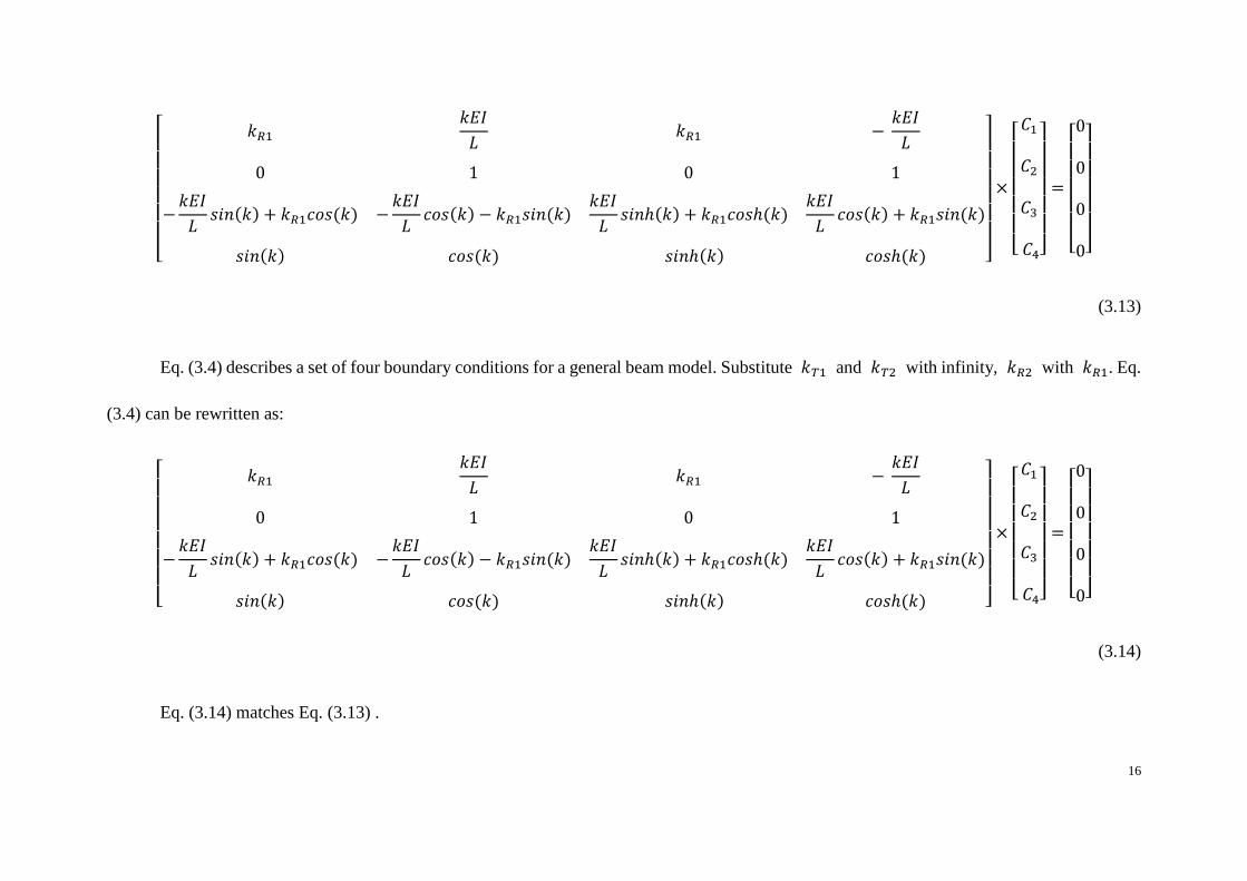
Eq. (3.4) describes a set of four boundary conditions for a general beam model. Substitute 𝑘𝑇1 and 𝑘𝑇2 with infinity, 𝑘𝑅2 with 𝑘𝑅1. Eq.

(3.4) can be rewritten as:

[ 𝑘𝑅1

𝑘𝐸𝐼

𝐿𝑘𝑅1 −

𝑘𝐸𝐼

𝐿

0 1 0 1

−𝑘𝐸𝐼

𝐿𝑠𝑖𝑛(𝑘) + 𝑘𝑅1𝑐𝑜𝑠(𝑘) −

𝑘𝐸𝐼

𝐿𝑐𝑜𝑠(𝑘) − 𝑘𝑅1𝑠𝑖𝑛(𝑘)

𝑘𝐸𝐼

𝐿𝑠𝑖𝑛ℎ(𝑘) + 𝑘𝑅1𝑐𝑜𝑠ℎ(𝑘)

𝑘𝐸𝐼

𝐿𝑐𝑜𝑠(𝑘) + 𝑘𝑅1𝑠𝑖𝑛(𝑘)


×

[ 𝐶1

𝐶2

𝐶3

𝐶4]

=

[ 0

0

0

0]

(3.14)

Eq. (3.14) matches Eq. (3.13) .

17

When 𝑘𝑇1 and 𝑘𝑇2 approach infinity, 𝑘𝑅1 and 𝑘𝑅2 go zero, the beam becomes a

simply supported beam, as shown in Figure 3.4.

𝑘𝑇1 = 𝑘𝑇2 = ∞, 𝑘𝑅1 = 𝑘𝑅2 = 0

Figure 3.4: A Simply Supported Euler-Bernoulli Beam

Eq. (3.13) can be reduced to:

[ 0

𝑘𝐸𝐼

𝐿0 −

𝑘𝐸𝐼

𝐿

0 1 0 1

−𝑘𝐸𝐼

𝐿𝑠𝑖𝑛(𝑘) −

𝑘𝐸𝐼

𝐿𝑐𝑜𝑠(𝑘)

𝑘𝐸𝐼

𝐿𝑠𝑖𝑛ℎ(𝑘)

𝑘𝐸𝐼



× [

𝐶1

𝐶2

𝐶3

𝐶4

] = [

0000

]

(3.15)

The frequency equation can be simplified to:

𝑠𝑖𝑛 (𝑘) = 0 (3.16)

Eq. (3.16) is verified with Timoshenko’s (1990) results.

18

Chapter 4 Free Vibration of Timoshenko Beams

4.1 Timoshenko Beams under Free Vibrations

In chapter 3, free vibrations of Euler-Bernoulli beams have been studied. Euler-Bernoulli

beam theory is accurate only for slender beams. Timoshenko beams theory takes into account of

the shear deformation and the effects of rotary inertia. It is more accurate than Euler-Bernoulli

beams for frequency calculations of deep beams, especially when beams are vibrating at higher

mode.

The governing equations for Timoshenko Beams are given in Vibration Problem in

Engineering (Timoshenko 1990):

𝐸𝐼𝜕2𝜑

𝜕𝑥2 + 𝐾𝐴𝐺 (𝜕𝑦

𝜕𝑥− 𝜑) − 𝜌𝐼

𝜕2𝜑

𝜕𝑡2 = 0 (4.1)


𝜕𝑡2 + 𝐾𝐴𝐺 (𝜕2𝑦

𝜕𝑥2 −𝜕𝜑

𝜕𝑥) = 0 (4.2)

K is the numerical shape factor. y represents the lateral displacement. 𝜑 denotes the angle

of rotation of the cross section due to bending.

Sign conventions for positive moment and positive shear are defined as:

+M +V

Moment and shear can be expressed as:

Figure 4.1: Sign Convention for Timoshenko Beams




19

𝑀(𝑥, 𝑡) = 𝐸𝐼𝜕𝜑

𝜕𝑥 (4.3)

𝑉(𝑥, 𝑡) = −𝐾𝐴𝐺 (𝜕𝑦

𝜕𝑥− 𝜑) (4.4)

After applying of separation of variable methods (Huang 1961), Eqs. (4.1) and (4.2) can

be stated as:

𝐸𝐼𝜕4𝑦

𝜕𝑥4+ 𝜌𝐴

𝜕2𝑦

𝜕𝑡2− (

𝐸𝐼𝜌

𝐾𝐺+ 𝜌𝐼)

𝜕4𝑦

𝜕𝑥2𝜕𝑡2+ 𝜌𝐼

𝜌

𝐾𝐺

𝜕4𝑦

𝜕𝑡4 = 0 (4.5)

EI𝜕4𝜑

𝜕𝑥4 + 𝜌𝐴𝜕2𝜑

𝜕𝑡2 − ( 𝐸𝐼𝜌

𝐾𝐺 + 𝜌𝐼)

𝜕4𝜑

𝜕𝑥2𝜕𝑡2 + 𝜌𝐼 𝜌

𝐾𝐺

𝜕4𝜑

𝜕𝑡4 = 0 (4.6)

Transverse deflection y, and bending angle 𝜑, can be written in term of dimensionless

length 𝜉, and time t:

𝑦 = 𝑌 (𝜉) 𝑒𝑖𝜔𝑡 (4.7)

𝜑 = 𝛹 (𝜉) 𝑒𝑖𝜔𝑡 (4.8)

Let’s introduce three variables b, r, and s:

𝑏2 = 𝜌𝐴𝐿4𝜔2 / (𝐸𝐼) (4.9)

𝑟2 = 𝐼/(𝐴𝐿2) (4.10)

𝑠2 = 𝐸𝐼/(𝐾𝐴𝐺𝐿2) (4.11)

Substitute Eqs. (4.7) and (4.8) into Eqs. (4.5) and (4.6), then omit the 𝑒𝑖𝜔𝑡 on both sides

of equations

𝑌𝐼𝑉 + 𝑏2(𝑟2 + 𝑠2) 𝑌′′ − 𝑏2(1 − 𝑟2𝑠2𝑏2)𝑌 = 0 (4.12)

𝛹𝐼𝑉 + 𝑏2(𝑟2 + 𝑠2) 𝛹′′ − 𝑏2(1 − 𝑟2𝑠2𝑏2)𝛹 = 0 (4.13)

20

Assume Y equals to 𝑒𝜆𝜉 . Therefore, Eq. (4.12) becomes

𝜆4 × 𝑒𝜆𝜉 + 𝑏2(𝑟2 + 𝑠2) 𝑒𝜆𝜉 − 𝑏2(1 − 𝑟2𝑠2𝑏2) 𝑒𝜆𝜉 = 0 (4.14)

Eliminate 𝑒𝜆𝜉 on both sides. Eq. (4.14) can be reduced to:

𝜆4 + 𝜆2𝑏2(𝑟2 + 𝑠2) − 𝑏2(1 − 𝑟2𝑠2𝑏2) = 0 (4.15)

Let H equals to 𝜆2, then Eq. (4.15) can be written as

𝐻2 + 𝑏2(𝑟2 + 𝑠2) 𝐻 − (1 − 𝑟2𝑠2𝑏2) = 0 (4.16)

Two roots of Eq. (4.16) are

𝐻1 =𝑏2

2[−(𝑟2 + 𝑠2) + √(𝑟2 − 𝑠2)2 +

4

𝑏2 ] (4.17a)

𝐻2 =𝑏2

2[−(𝑟2 + 𝑠2) − √(𝑟2 − 𝑠2)2 +

4

𝑏2] (4.17b)

When √(𝑟2 − 𝑠2)2 +4

𝑏2 is greater than (𝑟2 + 𝑠2), 𝐻1 is positive. The four roots of Eq.

(4.15) are

𝜆1 = 𝑏√1

2[− (𝑟2 + 𝑠2) + √(𝑟2 − 𝑠2)2 +

4

𝑏2 ] (4.18a)

𝜆2 = − 𝑏√1

2[−( 𝑟2 + 𝑠2) + √(𝑟2 − 𝑠2)2 +

4

𝑏2 ] (4.18b)

𝜆3 = 𝑖 𝑏√1

2[(𝑟2 + 𝑠2) + √(𝑟2 − 𝑠2)2 +

4

𝑏2 ] (4.18c)

21

𝜆4 = −𝑖 𝑏 √1

2[ (𝑟2 + 𝑠2) + √(𝑟2 − 𝑠2)2 +

4

𝑏2 ] (4.18d)

Let’s define 𝛼 and 𝛽

𝛼 = √1

2[−(𝑟2 + 𝑠2) + √(𝑟2 − 𝑠2)2 +

4

𝑏2 ] 4.19

𝛽 = √1

2[(𝑟2 + 𝑠2) + √(𝑟2 − 𝑠2)2 +

4

𝑏2 ] 4.20

Therefore, 𝜆1 to 𝜆4 can rewritten as

𝜆1 = 𝑏𝛼, 𝜆2 = −𝑏𝛼, 𝜆3 = 𝑏𝛽i, 𝜆4 = −𝑏𝛽𝑖 (4.21)

Y can be written as

𝑌( ) = 𝐶1𝑒𝑏𝛼𝜉 + 𝐶2 𝑒−𝑏𝛼𝜉 + 𝐶3 𝑒𝑏𝛽𝜉𝑖 + 𝐶4 𝑒−𝑏𝛽𝜉𝑖 (4.22)

Eq. (4.22) can be rewritten as

𝑌 ( ) = 𝐶1cosh(𝑏𝛼𝜉) + 𝐶2 𝑠𝑖𝑛ℎ(𝑏𝛼𝜉) + 𝐶3 𝑐𝑜𝑠(𝑏𝛽𝜉) + 𝐶4 𝑠𝑖𝑛(𝑏𝛽𝜉) (4.23)

Similarly, the bending angle can be 𝛹 derived. 𝛹 can be expressed as

𝛹(𝜉) = 𝐷1 𝑠𝑖𝑛ℎ (𝑏𝛼𝜉) + 𝐷2 𝑐𝑜𝑠ℎ (𝑏𝛼𝜉) + 𝐷3 𝑠𝑖𝑛 (𝑏𝛽𝜉) + 𝐷4 𝑐𝑜𝑠 (𝑏𝛽𝜉) (4.24)

Eq. (4.23) and Eq. (4.24) can be related to each other by the Eq. (4.6),

𝐶1 =𝐿𝛼

𝑏(𝛼2+𝑠2)𝐷1 𝐶2 =

𝐿𝛼

𝑏(𝛼2+𝑠2)𝐷2

22

𝐶3 = −𝐿𝛽

𝑏(𝛽2−𝑠2)𝐷3 𝐶4 =

𝐿𝛽

𝑏(𝛽2−𝑠2)𝐷4 (4.25)

Deflection Y can be written as 𝑌(𝜉) =𝐿𝛼

𝑏(𝛼2+𝑠2)𝐷1 𝑐𝑜𝑠ℎ(𝑏𝛼𝜉) +

𝐿𝛼

𝑏(𝛼2+𝑠2)𝐷2𝑠𝑖𝑛ℎ (𝑏𝛼𝜉) −

𝐿𝛽

𝑏(𝛽2−𝑠2)𝐷3𝑐𝑜𝑠 (𝑏𝛽𝜉) +

𝐿𝛽

𝑏(𝛽2−𝑠2)𝐷4𝑠𝑖𝑛 (𝑏𝛽𝜉) (4.26)

When √(𝑟2 − 𝑠2)2 +4

𝑏2 is less than (𝑟2 + 𝑠2), 𝐻1 is a negative number. Following

the same derivation procedure, Y and 𝛹 can be calculated as

𝑌(𝜉) = 𝐶1′𝑐𝑜𝑠 (𝑏µ𝜉) + 𝐶2′ 𝑠𝑖𝑛 (𝑏µ𝜉) + 𝐶3′ 𝑐𝑜𝑠 (𝑏𝛽𝜉) + 𝐶4′ 𝑠𝑖𝑛 (𝑏𝛽𝜉) (4.27)

𝛹(𝜉) = 𝐷1′ 𝑠𝑖𝑛 (𝑏µ𝜉) + 𝐷2′ 𝑐𝑜𝑠 (𝑏µ𝜉) + 𝐷3′ 𝑠𝑖𝑛 (𝑏𝛽𝜉) + 𝐷4′ 𝑐𝑜𝑠 (𝑏𝛽𝜉) (4.28)

where µ is√1

2[(𝑟2 + 𝑠2) − √(𝑟2 − 𝑠2)2 +

4

𝑏2 ].

4.2 Natural Frequencies and Mode Shapes of a Timoshenko Beam with Various Boundary

Conditions

In this chapter, a more general beam model is studied, which is a beam with two different

rotational springs and two different verticals spring on ends. It has the ability to simulate all kinds

of beam ends conditions. To the best of our knowledge, the frequencies and modes shapes of this

beam model is not available in the literature. Below is the sketch of the beam:

23

Figure 4.2: A Timoshenko Beam with Two Rotational Springs and Two Vertical Springs

Majkut (2009) discussed the frequencies and mode shapes of a Timoshenko beam with two

identical vertical springs and two identical rotational springs at both ends, which is not as general

as the beam studied in this section. However, he made a crucial mistake when he calculated the

moment in page 199. The moment should be caused by pure bending angle alone, instead of both

pure bending angle and shear angle.

The boundary conditions for this beam are

𝑀⃒𝜉=0 = 𝑘𝑅1𝛹⃒𝜉=0 𝑉⃒𝜉=0 = −𝑘𝑇1𝑌⃒𝜉=0

𝑀⃒𝜉=1 = −𝑘𝑅2𝛹⃒𝜉=1 𝑉⃒𝜉=1 = 𝑘𝑇2𝑌⃒𝜉=1 (4.29)

Deflection Y, bending angle 𝛹, moment M, and shear force V, can be calculated as below

24

𝑌(𝜉) = 𝐿𝛼

𝑏(𝛼2+𝑠2)𝐷1 cosh(𝑏𝛼𝜉) +

𝐿𝛼

𝑏(𝛼2+𝑠2)𝐷2 sinh(𝑏𝛼𝜉) −

𝐿𝛽

𝑏(𝛽2−𝑠2)𝐷3 cos(𝑏𝛽𝜉) +

𝐿𝛽

𝑏(𝛽2−𝑠2)𝐷4𝑠𝑖𝑛(𝑏𝛽𝜉) (4.30)

𝛹(𝜉) = 𝐷1 𝑠𝑖𝑛ℎ(𝑏𝛼𝜉) + 𝐷2 𝑐𝑜𝑠ℎ(𝑏𝛼𝜉) + 𝐷3 𝑠𝑖𝑛(𝑏𝛽𝜉) + 𝐷4 𝑐𝑜𝑠(𝑏𝛽𝜉) (4.31)

𝑀(𝜉) =𝐸𝐼𝑏𝛼

𝐿𝑐𝑜𝑠ℎ(𝑏𝛼𝜉)𝐷1 +

𝐸𝐼𝑏𝛼

𝐿 𝑠𝑖𝑛ℎ(𝑏𝛼𝜉)𝐷2 +

𝐸𝐼𝑏𝛽

𝐿 𝑐𝑜𝑠(𝑏𝛽𝜉)𝐷3 −

𝐸𝐼𝑏𝛽

𝐿𝑠𝑖𝑛 (𝑏𝛽𝜉)𝐷4 (4.32)

𝑉(𝜉) = 𝐾𝐴𝐺 ( 𝑠2

𝑠2+𝑎2𝑠𝑖𝑛ℎ (𝑏𝛼𝜉)𝐷1 +

𝑠2

𝑠2+𝑎2𝑐𝑜𝑠ℎ (𝑏𝛼𝜉)𝐷2 −

𝑠2

𝛽2−𝑠2 𝑠𝑖𝑛 (𝑏𝛽𝜉)𝐷3 −

𝑠2

𝛽2−𝑠2𝑐𝑜𝑠 (𝑏𝛽𝜉) (4.33)

Plug Eqs. (4.30) to (4.33) into boundary equations,

[

−𝑘𝑇1𝐿𝛼

𝑏(𝛼2 + 𝑠2) −𝐾𝐴𝐺𝑠2

(𝛼2 + 𝑠2)

𝑘𝑇1𝐿𝛽

𝑏(𝛽2 − 𝑠2)

𝐾𝐴𝐺𝑠2

(𝛽2 − 𝑠2)

𝐸𝐼𝑏𝛼

𝐿−𝑘𝑅1

𝐸𝐼𝑏𝛽

𝐿−𝑘𝑅1

𝐾𝐴𝐺𝑠2𝑏 𝑠𝑖𝑛ℎ(𝑏𝛼) − 𝑘𝑇2𝐿𝛼 cosh(𝑏𝛼)

𝑏(𝛼2 + 𝑠2)

𝐾𝐴𝐺𝑠2𝑏𝑐𝑜𝑠ℎ(𝑏𝛼) − 𝑘𝑇2𝐿𝛼 sinh(𝑏𝛼)

𝑏(𝛼2 + 𝑠2) −𝐾𝐴𝐺𝑠2𝑏𝑠𝑖𝑛(𝑏𝛽) + 𝑘𝑇2𝐿𝛽 cos(𝑏𝛼)

𝑏(𝛽2 − 𝑠2)

−𝐾𝐴𝐺𝑠2𝑏𝑐𝑜𝑠(𝑏𝛽) − 𝑘𝑇2𝐿𝛽 sin(𝑏𝛼)

𝑏(𝛽2 − 𝑠2)

𝐸𝐼𝑏𝛼 𝑐𝑜𝑠ℎ(𝑏𝛼) + 𝑘𝑅2𝐿𝑠𝑖𝑛ℎ(𝑏𝛼)

𝐿 𝐸𝐼𝑏𝛼 𝑠𝑖𝑛ℎ(𝑏𝛼) + 𝑘𝑅2𝐿𝑐𝑜𝑠ℎ(𝑏𝛼)

𝐿

𝐸𝐼𝑏𝛽 𝑐𝑜𝑠(𝑏𝛼) + 𝑘𝑅2𝐿𝑠𝑖𝑛(𝑏𝛼)

𝐿 −𝐸𝐼𝑏𝛽 𝑠𝑖𝑛(𝑏𝛼) + 𝑘𝑅2𝐿𝑐𝑜𝑠(𝑏𝛼)

𝐿 ]

×

[ 𝐷1

𝐷2

𝐷3

𝐷4]

=

[ 0

0

0

0]

(4.34)

25

The frequency equation can be calculated by


𝑏(𝛼2+𝑠2)× [−𝑘𝑅1 ×

−𝐾𝐴𝐺𝑠2𝑏𝑠𝑖𝑛(𝑏𝛽)+𝑘𝑇2𝐿𝛽 𝑐𝑜𝑠(𝑏𝛼)

𝑏(𝛽2−𝑠2)×

−𝐸𝐼𝑏𝛽 𝑠𝑖𝑛(𝑏𝛼)+𝑘𝑅2𝐿𝑐𝑜𝑠(𝑏𝛼)

𝐿+


𝐿×

−𝐾𝐴𝐺𝑠2𝑏𝑐𝑜𝑠(𝑏𝛽)−𝑘𝑇2𝐿𝛽 𝑠𝑖𝑛(𝑏𝛼)

𝑏(𝛽2−𝑠2)×

𝐸𝐼𝑏𝛼 𝑠𝑖𝑛ℎ(𝑏𝛼)+𝑘𝑅2𝐿𝑐𝑜𝑠ℎ(𝑏𝛼)

𝐿– 𝑘𝑅1 ×

𝐾𝐴𝐺𝑠2𝑏𝑐𝑜𝑠ℎ(𝑏𝛼)−𝑘𝑇2𝐿𝛼 𝑠𝑖𝑛ℎ(𝑏𝛼)

𝑏(𝛼2+𝑠2)×

𝐸𝐼𝑏𝛽 𝑐𝑜𝑠(𝑏𝛼)+𝑘𝑅2𝐿𝑠𝑖𝑛(𝑏𝛼)

𝐿+ 𝑘𝑅1 ×


𝑏(𝛽2−𝑠2)×


𝐿+ 𝑘𝑅1 ×


𝑏(𝛽2−𝑠2)×


𝐿−

𝐸𝐼𝑏𝛽

𝐿×

𝐾𝐴𝐺𝑠2𝑏𝑐𝑜𝑠ℎ(𝑏𝛼)−𝑘𝑇2𝐿𝛼 𝑠𝑖𝑛ℎ(𝑏𝛼)

𝑏(𝛼2+𝑠2)×


𝐿] −

−𝐾𝐴𝐺𝑠2

(𝛼2+𝑠2)× [

𝐸𝐼𝑏𝛼

𝐿×


𝑏(𝛽2−𝑠2)×


𝐿+

𝐸𝐼𝑏𝛽

𝐿×

−𝐾𝐴𝐺𝑠2𝑏𝑐𝑜𝑠(𝑏𝛽)−𝑘𝑇2𝐿𝛽𝑠𝑖𝑛 (𝑏𝛼)

𝑏(𝛽2−𝑠2)×

𝐸𝐼𝑏𝛼𝑐𝑜𝑠ℎ(𝑏𝛼)+𝑘𝑅2𝐿𝑠𝑖𝑛ℎ(𝑏𝛼)

𝐿− 𝑘𝑅1 ×

𝐾𝐴𝐺𝑠2𝑏𝑠𝑖𝑛ℎ(𝑏𝛼)−𝑘𝑇2𝐿𝛼𝑐𝑜𝑠ℎ (𝑏𝛼)

𝑏(𝛼2+𝑠2)×


𝐿+ 𝑘𝑅1 ×

−𝐾𝐴𝐺𝑠2𝑏𝑠𝑖𝑛(𝑏𝛽)+𝑘𝑇2𝐿𝛽𝑐𝑜𝑠 (𝑏𝛼)

𝑏(𝛽2−𝑠2)

×𝐸𝐼𝑏𝛼𝑐𝑜𝑠ℎ(𝑏𝛼)+𝑘𝑅2𝐿𝑠𝑖𝑛ℎ(𝑏𝛼)

𝐿−

𝐸𝐼𝑏𝛼

𝐿×


𝑏(𝛽2−𝑠2)×


𝐿−

𝐸𝐼𝑏𝛽

𝐿×

𝐾𝐴𝐺𝑠2𝑏 𝑠𝑖𝑛ℎ(𝑏𝛼)−𝑘𝑇2𝐿𝛼𝑐𝑜𝑠ℎ (𝑏𝛼)

𝑏(𝛼2+𝑠2)×


𝐿] +

𝑘𝑇1𝐿𝛽

𝑏(𝛽2−𝑠2)× [

𝐸𝐼𝑏𝛼

𝐿×

𝐾𝐴𝐺𝑠2𝑏𝑐𝑜𝑠ℎ(𝑏𝛼)−𝑘𝑇2𝐿𝛼𝑠𝑖𝑛ℎ (𝑏𝛼)

𝑏(𝛼2+𝑠2)×


𝐿− 𝑘𝑅1 ×


𝑏(𝛽2−𝑠2)×

𝐸𝐼𝑏𝛼 𝑐𝑜𝑠ℎ(𝑏𝛼)+𝑘𝑅2𝐿𝑠𝑖𝑛ℎ(𝑏𝛼)

𝐿− 𝑘𝑅1 ×


𝑏(𝛼2+𝑠2)×


𝐿+𝑘𝑅1 ×


𝑏(𝛼2+𝑠2)×


𝐿−

𝐸𝐼𝑏𝛼

𝐿×


𝑏(𝛽2−𝑠2)×


𝐿+ 𝑘𝑅1 ×


𝑏(𝛼2+𝑠2)×


𝐿 ] −

𝐾𝐴𝐺𝑠2

(𝛽2−𝑠2)× [

𝐸𝐼𝑏𝛼

𝐿×


𝑏(𝛼2+𝑠2) ×


𝐿− 𝑘𝑅1 ×

26


𝑏(𝛽2−𝑠2)×


𝐿+

𝐸𝐼𝑏𝛽

𝐿×


𝑏(𝛼2+𝑠2)×


𝐿−

𝐸𝐼𝑏𝛽

𝐿×

𝐾𝐴𝐺𝑠2𝑏𝑐𝑜𝑠ℎ(𝑏𝛼)− 𝑘𝑇2𝐿𝛼𝑠𝑖𝑛ℎ (𝑏𝛼)

𝑏(𝛼2+𝑠2)×


𝐿−

𝐸𝐼𝑏𝛼

𝐿×

−𝐾𝐴𝐺𝑠2𝑏𝑠𝑖𝑛(𝑏𝛽)+𝑘𝑇2𝐿𝛽𝑐𝑜𝑠 (𝑏𝛼)

𝑏(𝛽2−𝑠2)×


𝐿+ 𝑘𝑅1 ×

𝐾𝐴𝐺𝑠2𝑏 𝑠𝑖𝑛ℎ(𝑏𝛼)− 𝑘𝑇2𝐿𝛼𝑐𝑜𝑠ℎ (𝑏𝛼)

𝑏(𝛼2+𝑠2)×


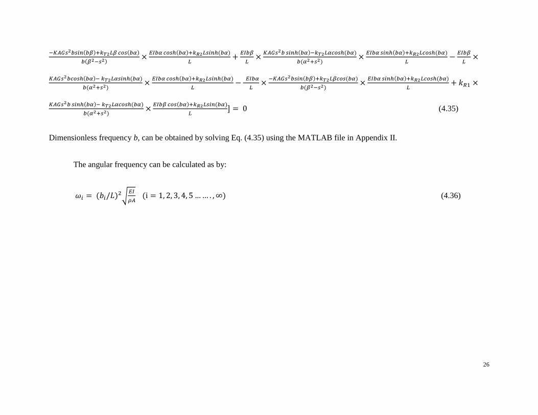
𝐿] = 0 (4.35)

Dimensionless frequency b, can be obtained by solving Eq. (4.35) using the MATLAB file in Appendix II.

The angular frequency can be calculated as by:

𝜔𝑖 = (𝑏𝑖/𝐿)2√𝐸𝐼

𝜌𝐴 (i = 1, 2, 3, 4, 5 …… . ,∞) (4.36)

27

4.3 Natural Frequencies and Mode Shapes of a Cantilever Timoshenko Beam with a

Rotational Spring and a Vertical Spring

In this section, the free vibration of a cantilever Timoshenko beam with a rotational spring

and a vertical spring is analyzed. The beam is demonstrated below:

Figure 4.3: A Cantilever Timoshenko Beam with a Rotational Spring and a Vertical Spring


𝑀⃒𝜉=0 = 𝑘𝑅1𝛹⃒𝜉=0 , 𝑀⃒𝜉=1 = 0

𝑉⃒𝜉=0 = −𝑘𝑇1𝑌⃒𝜉=0, 𝑉⃒𝜉=1 = 0 (4.37)

Plug Eqs. (4.30) to (4.33) into boundary equations,

[



(𝛼2 + 𝑠2)

𝑘𝑇1𝐿𝛽

𝑏(𝛽2 − 𝑠2)

𝐾𝐴𝐺𝑠2

(𝛽2 − 𝑠2)

𝐸𝐼𝑏𝛼

𝐿−𝑘𝑅1

𝐸𝐼𝑏𝛽

𝐿−𝑘𝑅1

𝐾𝐴𝐺𝑠2

𝑠2 + 𝑎2𝑠𝑖𝑛ℎ (𝑏𝛼)

𝐾𝐴𝐺𝑠2

𝑠2 + 𝑎2𝑐𝑜𝑠ℎ (𝑏𝛼) −

𝐾𝐴𝐺𝑠2

𝛽2 − 𝑠2 𝑠𝑖𝑛 (𝑏𝛽) −

𝐾𝐴𝐺𝑠2

𝛽2 − 𝑠2 𝑐𝑜𝑠 (𝑏𝛽)

𝐸𝐼𝑏𝛼

𝐿𝑐𝑜𝑠ℎ(𝑏𝛼)

𝐸𝐼𝑏𝛼

𝐿 𝑠𝑖𝑛ℎ (𝑏𝛼)

𝐸𝐼𝑏𝛽

𝐿 𝑐𝑜𝑠 (𝑏𝛽) −

𝐸𝐼𝑏𝛽

𝐿 𝑠𝑖𝑛 (𝑏𝛽) ]

28

×

[ 𝐶1

𝐶2

𝐶3

𝐶4]

=

[ 0

0

0

0]

(4.38)

The boundary conditions of the general Timoshenko beam under free vibrations are

described by a set of four homogenous equations in Eq. (4.34) . Let 𝑘𝑇2 and 𝑘𝑅2 equal to zero,

the beam becomes to a cantilever beam with a rotational spring and a vertical spring, as shown in

Figure 4.3. Eq. (4.34) can be simplified to be:

[



(𝛼2 + 𝑠2)

𝑘𝑇1𝐿𝛽

𝑏(𝛽2 − 𝑠2)

𝐾𝐴𝐺𝑠2

(𝛽2 − 𝑠2)

𝐸𝐼𝑏𝛼

𝐿−𝑘𝑅1

𝐸𝐼𝑏𝛽

𝐿−𝑘𝑅1

𝐾𝐴𝐺𝑠2


𝐾𝐴𝐺𝑠2


𝐾𝐴𝐺𝑠2

𝛽2 − 𝑠2 𝑠𝑖𝑛 (𝑏𝛽) −

𝐾𝐴𝐺𝑠2


𝐸𝐼𝑏𝛼


𝐸𝐼𝑏𝛼


𝐸𝐼𝑏𝛽


𝐸𝐼𝑏𝛽


×

[ 𝐶1

𝐶2

𝐶3

𝐶4]

=

[ 0

0

0

0]

(4.39)

Eq. (4.39) is identical to Eq. (4.38) .

The frequency equation of the cantilever beam with a rotational spring and a vertical spring

can be written as:

29

𝑏2𝐸𝐼𝐾𝐴𝐺𝑆2 [2 − 2 𝑐𝑜𝑠ℎ(𝑏𝛼) 𝑐𝑜𝑠(𝑏𝛽) +𝑏[𝑏2𝑟2(𝑟2−𝑠2)+(3𝑟2−𝑠2)

√1−𝑏2𝑟2𝑠2𝑠𝑖𝑛ℎ(𝑏𝛼) 𝑠𝑖𝑛(𝑏𝛽)] +

𝑘𝑅𝑘𝑇𝐿2 [2 + (𝑏2(𝑟2 − 𝑠2)2 + 2) 𝑐𝑜𝑠ℎ(𝑏𝛼) 𝑐𝑜𝑠(𝑏𝛽) −𝑏(𝑟2+𝑠2)

√1−𝑏2𝑟2𝑠2𝑠𝑖𝑛ℎ(𝑏𝑎) 𝑠𝑖𝑛(𝑏𝛽)] +

𝑘𝑇𝐸𝐼𝐿𝑏3(𝛼2 + 𝛽2)[𝛼(𝛼2 + 𝑠2) 𝑠𝑖𝑛ℎ(𝑏𝛼) 𝑐𝑜𝑠(𝑏𝛽) − 𝛽(𝛽2 − 𝑠2) 𝑐𝑜𝑠ℎ(𝑏𝛼) 𝑠𝑖𝑛(𝑏𝛽) −

𝑘𝑅𝐾𝐴𝐺𝐿𝑏3𝑠2 𝛼2+𝛽2

𝛼𝛽[𝛽(𝛽2 − 𝑠2) 𝑠𝑖𝑛ℎ(𝑏𝛼) 𝑐𝑜𝑠(𝑏𝛽) + 𝛼(𝛼2 + 𝑠2) 𝑐𝑜𝑠ℎ(𝑏𝛼) 𝑠𝑖𝑛(𝑏𝛽) = 0

(4.40)

Eq. (4.40) can be validated with Chen and Kiriakidis’s (2005) frequency equation.

Let 𝑘𝑇1 and 𝑘𝑅1 go to infinity, 𝑘𝑇2 and 𝑘𝑅2 equal to zero, the beam becomes a

cantilever beam.

Eq. (4.38) can be reduced to be:

[

−𝐿𝛼

𝑏(𝛼2 + 𝑠2)0

𝐿𝛽

𝑏(𝛽2 − 𝑠2)0

0 −1 0 −1

𝐾𝐴𝐺𝑠2


𝐾𝐴𝐺𝑠2


𝐾𝐴𝐺𝑠2

𝛽2 − 𝑠2 𝑠𝑖𝑛 (𝑏𝛽) −

𝐾𝐴𝐺𝑠2


𝐸𝐼𝑏𝛼


𝐸𝐼𝑏𝛼


𝐸𝐼𝑏𝛽


𝐸𝐼𝑏𝛽


×

[ 𝐶1

𝐶2

𝐶3

𝐶4]

=

[ 0

0

0

0]

(4.41)

30

The frequency of the cantilever beam can be calculated by

2 + [ 𝑏2 (𝑟2 − 𝑠2)2 + 2]𝑐𝑜𝑠ℎ(𝑏𝛼)𝑐𝑜𝑠(𝑏𝛽) −𝑏 (𝑟2+ 𝑠2)

(1−𝑟2 𝑠2𝑏2) 𝑠𝑖𝑛ℎ(𝑏𝛼)𝑠𝑖𝑛(𝑏𝛽) = 0 (4.42)

Eq. (4.42) matches Huang’s (1961) results.

4.4 Natural Frequencies and Mode Shapes of a Timoshenko Beam with Two Rotational

Springs and Two Fixed Vertical Supports

The natural frequencies and mode shapes of a Timoshenko beam with two rotational spring

and two fixed vertical supports are derived in this section. Blow is the sketch of the beam:

Figure 4.4: A Timoshenko Bernoulli Beam with Two Rotational Springs

The boundary conditions of the beam are:

𝑀⃒𝜉=0 = 𝑘𝑅1𝛹⃒𝜉=0

𝑀⃒𝜉=1 = −𝑘𝑅1𝛹⃒𝜉=1

𝑌⃒𝜉=0 = 0

𝑌⃒𝜉=1 = 0 (4.43)

𝑘𝑇1 = 𝑘𝑇2 = ∞, 𝑘𝑅1 = 𝑘𝑅2

𝑘𝑇1 = 𝑘𝑇2 = ∞, 𝑘𝑅1 = 𝑘𝑅2

31

Substitute Eqs. (4.30) to (4.33) into boundary equations,

[

𝐿𝛼

𝑏(𝛼2+𝑠2)0 −

𝐿𝛽

𝑏𝑖(𝛽2−𝑠2)

0

𝐸𝐼𝑏𝛼

𝐿−𝑘𝑅1

𝐸𝐼𝑏𝛽

𝐿−𝑘𝑅1

𝐿𝛼

𝑏(𝛼2+𝑠2)𝑐𝑜𝑠ℎ(𝑏𝛼)

𝐿𝛼

𝑏(𝛼2+𝑠2)𝑠𝑖𝑛ℎ(𝑏𝛼) −

𝐿𝛽

𝑏(𝛽2−𝑠2)𝑐𝑜𝑠(𝑏𝛽)

𝐿𝛽

𝑏(𝛽2−𝑠2)𝑠𝑖𝑛(𝑏𝛽)

𝐸𝐼𝑏𝛼 𝑐𝑜𝑠ℎ(𝑏𝛼)+𝑘𝑅1 𝐿𝑠𝑖𝑛ℎ(𝑏𝛼)

𝐿

𝐸𝐼𝑏𝛼 𝑠𝑖𝑛ℎ(𝑏𝛼)+𝑘𝑅1 𝐿𝑐𝑜𝑠ℎ(𝑏𝛼)

𝐿

𝐸𝐼𝑏𝛽 𝑐𝑜𝑠(𝑏𝛼)+𝑘𝑅1 𝐿𝑠𝑖𝑛(𝑏𝛼)

𝐿

−𝐸𝐼𝑏𝛽 𝑠𝑖𝑛(𝑏𝛼)+𝑘𝑅1 𝐿𝑐𝑜𝑠(𝑏𝛼)

𝐿 ]

×

[ 𝐷1

𝐷2

𝐷3

𝐷4]

=

[ 0

0

0

0]

(4.44)

Substitute 𝑘𝑇1 and 𝑘𝑇2 with infinity, 𝑘𝑅2 with 𝑘𝑅1 into Eq. (4.42) ,

[

𝐿𝛼

𝑏(𝛼2+𝑠2)0 −

𝐿𝛽

𝑏𝑖(𝛽2−𝑠2)

0

𝐸𝐼𝑏𝛼

𝐿−𝑘𝑅1

𝐸𝐼𝑏𝛽

𝐿−𝑘𝑅1

𝐿𝛼


𝐿𝛼


𝐿𝛽


𝐿𝛽

𝑏(𝛽2−𝑠2)𝑠𝑖𝑛(𝑏𝛽)

𝐸𝐼𝑏𝛼 𝑐𝑜𝑠ℎ(𝑏𝛼)+𝑘𝑅1 𝐿𝑠𝑖𝑛ℎ(𝑏𝛼)

𝐿

𝐸𝐼𝑏𝛼 𝑠𝑖𝑛ℎ(𝑏𝛼)+𝑘𝑅1 𝐿𝑐𝑜𝑠ℎ(𝑏𝛼)

𝐿

𝐸𝐼𝑏𝛽 𝑐𝑜𝑠(𝑏𝛼)+𝑘𝑅1 𝐿𝑠𝑖𝑛(𝑏𝛼)

𝐿

−𝐸𝐼𝑏𝛽 𝑠𝑖𝑛(𝑏𝛼)+𝑘𝑅1 𝐿𝑐𝑜𝑠(𝑏𝛼)

𝐿 ]

×

[ 𝐷1

𝐷2

𝐷3

𝐷4]

=

[ 0

0

0

0]

(4.45)

Eq. (4.43) matches Eq. (4.44) .

32

The frequency equation of the beam can be written as:

𝐿𝛼

𝑏(𝛼2+𝑠2)× (𝑘𝑅1 ×

𝐿𝛽

𝑏(𝛽2−𝑠2)cos(𝑏𝛽) ×

−𝐸𝐼𝑏𝛽𝑠𝑖𝑛(𝑏𝛼)+𝑘𝑅1𝐿𝑐𝑜𝑠(𝑏𝛼)

𝐿+

𝐸𝐼𝑏𝛽𝐿

×𝐿𝛽

𝑏(𝛽2−𝑠2)× 𝑠𝑖𝑛 (𝑏𝛽) ×


𝐿 + 𝑘𝑅1 ×

𝐿𝛼

𝑏(𝛼2+𝑠2)𝑠𝑖𝑛ℎ (𝑏𝛼) ×

𝐸𝐼𝑏𝛽𝑐𝑜𝑠(𝑏𝛼)+𝑘𝑅1𝐿𝑠𝑖𝑛(𝑏𝛼)

𝐿− 𝑘𝑅1 ×

𝐿𝛽

𝑏(𝛽2−𝑠2) 𝑐𝑜𝑠 (𝑏𝛽) ×

𝐸𝐼𝑏𝛼𝑠𝑖𝑛ℎ(𝑏𝛼)+𝑘𝑅1𝐿𝑐𝑜𝑠ℎ(𝑏𝛼)

𝐿 −

1Rk ×𝐿𝛽

𝑏(𝛽2−𝑠2) 𝑠𝑖𝑛 (𝑏𝛽) ×


𝐿−

𝐸𝐼𝑏𝛽𝐿

×𝐿𝛼

𝑏(𝛼2+𝑠2) 𝑠𝑖𝑛ℎ (𝑏𝛼) ×


𝐿] −

𝐿𝛽

𝑏(𝛽2−𝑠2)× [

𝐸𝐼𝑏𝛼𝐿

×𝐿𝛼

𝑏(𝛼2+𝑠2)sinh (𝑏𝛼) ×


𝐿 +

1Rk × sin (𝑏𝛽) ×


𝐿 −

1Rk 𝐿𝛼

𝑏(𝛼2+𝑠2) cosh (𝑏𝛼) ×

𝐸𝐼𝑏𝛼𝑠𝑖𝑛ℎ(𝑏𝛼)+𝑘𝑅1𝐿𝑐𝑜𝑠ℎ(𝑏𝛼)

𝐿 +

1Rk ×

𝐿𝛼

𝑏(𝛼2+𝑠2) 𝑠𝑖𝑛ℎ (𝑏𝛼)


𝐿 −

𝐸𝐼𝑏𝛼𝐿

× 𝐿𝛽

𝑏(𝛽2−𝑠2) 𝑠𝑖𝑛 (𝑏𝛽) ×


𝐿 −

1Rk𝐿𝛼

𝑏(𝛼2+𝑠2)×

𝑐𝑜𝑠ℎ (𝑏𝛼) ×−𝐸𝐼𝑏𝛽𝑠𝑖𝑛(𝑏𝛼)+𝑘𝑅1𝐿𝑐𝑜𝑠(𝑏𝛼)

𝐿 = 0 (4.46)

Eq. (4.45) can be converted to Ross’s (1985) frequency equation by following his notations.

When 𝑘𝑇1 and 𝑘𝑇2 approach infinity, 𝑘𝑅1 and 𝑘𝑅2 go zero, the beam becomes a simply supported beam. Eq. (4.43) can be

reduced to

33

[

𝐿𝛼

𝑏(𝛼2+𝑠2)0 −

𝐿𝛽

𝑏(𝛽2−𝑠2)0

𝐸𝐼𝑏𝛼

𝐿0

𝐸𝐼𝑏𝛽

𝐿0

𝐿𝛼


𝐿𝛼


𝐿𝛽


𝐿𝛽

𝑏(𝛽2−𝑠2)sin (𝑏𝛽)

𝐸𝐼𝑏𝛼

𝐿cosh (𝑏𝛼)

𝐸𝐼𝑏𝛼

𝐿sinh (𝑏𝛼)

𝐸𝐼𝑏𝛽

𝐿cos (𝑏𝛽) −

𝐸𝐼𝑏𝛽

𝐿sin (bβ) ]

×

[ 𝐷1

𝐷2

𝐷3

𝐷4]

=

[ 0

0

0

0]

(4.47)

The frequency of the simply supported beam can be stated as

𝑠𝑖𝑛 (𝑏𝛽) = 0 (4.48)

Eq. (4.47) is identical to Huang’s (1961) results.

34

CHAPTER 5 Forced Vibrations of Euler-Bernoulli Beams

5.1 Deflection Curves of Forced Vibrations of Euler-Bernoulli Beams

In this section, the deflection curve of forced vibrations of Euler-Bernoulli beams with an

arbitrary exciting distributed force q(𝜉 ,t) are presented. q(𝜉 ,t) points upwards. The governing

equation for the Euler-Bernoulli beam is

𝐸𝐼

𝐿4

𝜕4𝑦

𝜕𝜉4 + 𝜌𝐴𝜕2𝑦

𝜕𝑡2 = 𝑞(𝜉, 𝑡) (5.1)

Apply Laplace transform to Eq. (5.1),

𝐸𝐼

𝐿4 𝑦𝐼𝑉(𝜉, 𝜔) − 𝜌𝐴𝜔2 𝑦(𝜉, 𝜔) = q(𝜉, 𝜔) (5.2)

The forced vibration shape of an Euler-Bernoulli beam can be written as a Green function

in order for the beam to be in a steady state:

𝑦(𝜉, 𝑡) = 𝐺(𝜉, 𝜉𝑓) 𝑒𝑥𝑝(𝑖𝜔𝑡) (5.3)

where 𝜉𝑓 is the point where the arbitrary force is applied at.

Eq. (5.2) can be rewritten as

𝐸𝐼

𝐿4 𝐺𝐼𝑉(𝜉, 𝜉𝑓) − 𝜌𝐴𝜔2 𝐺(𝜉, 𝜉𝑓) = 𝛿(𝜉 − 𝜉𝑓) (5.4)

35

In this section, the effects of internal damping and external damping are neglected. The

vibration functions derived in this section are for dimensionless frequencies b, lower than cut-off

frequency: √(𝑟2 − 𝑠2)2 +4

𝑏2 > (𝑟2 + 𝑠2), which can be rewritten as b <1

𝑟2𝑠2.

G (𝜉, 𝜉𝑓) is summation of two parts: homogenous solution, and particular solution.

𝐺 (𝜉, 𝜉𝑓) = 𝐺0(𝜉) + 𝐺1(𝜉, 𝜉𝑓) 𝐻(𝜉 − 𝜉𝑓) (5.5)

where 𝐻(𝜉 − 𝜉𝑓) is the step function. It has the property that when 𝜉 is smaller than 𝜉𝑓, the

function equals to 0; when 𝜉 is bigger than 𝜉𝑓, the function equals to 1.

𝐺0(𝜉) is the solution to homogeneous equation, which can be stated as:

𝐺0(𝜉) = 𝐶1 𝑠𝑖𝑛 (𝑘𝜉) + 𝐶2 𝑐𝑜𝑠 (𝑘𝜉) + 𝐶3 𝑠𝑖𝑛ℎ (𝑘𝜉) + 𝐶4 𝑐𝑜𝑠ℎ (𝑘𝜉) (5.6)

k is the dimensionless frequency, which can be written as:

k = (𝐸𝐼𝜔2𝐿4

𝜌𝐴)1/4

(5.7)

𝐺1(𝜉, 𝜉𝑓) is the solution to inhomogeneous equation, which can be written as:

𝐺1(𝜉, 𝜉𝑓) = 𝑃1 cosh[𝑘(𝜉 − 𝜉𝑓)] + 𝑃2 sinh[ 𝑘(𝜉 − 𝜉𝑓)] + 𝑃3 cos[ 𝑘(𝜉 − 𝜉𝑓)]

+ 𝑃4𝑠𝑖𝑛[ 𝑘(𝜉 − 𝜉𝑓)] (5.8)

From continuity conditions

𝐺(𝜉𝑓+, 𝜉𝑓) − 𝐺(𝜉𝑓

−, 𝜉𝑓) = 0 (5.9a)

𝛹(𝜉𝑓+

, 𝜉𝑓) − 𝛹(𝜉𝑓−

, 𝜉𝑓) = 0 (5.9b)

36

M(𝜉𝑓+

, 𝜉𝑓) − M(𝜉𝑓−

, 𝜉𝑓) = 0 (5.9c)

V(𝜉𝑓+

, 𝜉𝑓) − V(𝜉𝑓−

, 𝜉𝑓) = 1 (5.9d)

Bending slope 𝛹, moment M, and shear force V, can be calculated by:

𝛹 (𝜉, 𝜉𝑓) = 𝑑𝐺

𝑑𝑥 =

1

𝐿

𝑑𝐺

𝑑𝜉 (5.10)

M (𝜉, 𝜉𝑓) = EI 𝑑2𝐺

𝑑𝑥2 =

𝐸𝐼

𝐿2

𝑑2𝐺

𝑑𝜉2 (5.11)

V (𝜉, 𝜉𝑓) = EI 𝑑3𝐺

𝑑𝑥3 =

𝐸𝐼

𝐿3

𝑑3𝐺

𝑑𝜉3 (5.12)

Apply Eqs. (5.8), (5.10), (5.11), and (5.12), into continuity conditions. After simplification,

we get the following terms

𝑃1 + 𝑃3 = 0 (5.13a)

𝑘

𝐿 (𝑃2 + 𝑃4) = 0 (5.13b)

𝐸𝐼𝑘2

𝐿2 (𝑃1 − 𝑃3) = 0 (5.13c)

𝐸𝐼𝑘3

𝐿3 (𝑃2 − 𝑃4) = 1 (5.13d)

Therefore, the four terms can be solved, which are

𝑃1 = 0, 𝑃2 =𝐿3

2𝐸𝐼𝑘3 , 𝑃3 = 0, 𝑃4 = −

𝐿3

2𝐸𝐼𝑘3 (5.14)

The close-form expression of forced vibration shape can be written as

37

𝐺(𝜉, 𝜉𝑓) = 𝐶1 sin(𝑘𝜉) + 𝐶2 cos(𝑘𝜉) + 𝐶3 sinh(𝑘𝜉) + 𝐶4 cosh(𝑘𝜉) +𝐿3

2𝐸𝐼𝑘3 ×

𝑠𝑖𝑛ℎ[ 𝑘(𝜉 − 𝜉𝑓)]𝐻[𝑘(𝜉 − 𝜉𝑓)] − 𝐿3

2𝐸𝐼𝑘3 𝑠𝑖𝑛[ 𝑘(𝜉 − 𝜉𝑓))] 𝐻(𝑘(𝜉 − 𝜉𝑓))]

(5.15)

5.2 Forced Vibrations of Euler-Bernoulli Beams with Two Different Rotational Springs and

Two Different Vertical Springs

A highly simply and general beam model is set up with two different rotational springs and

two vertical springs at both ends. The sketch has been presented Figure 3.1. To the best of my

knowledge, the force vibration of the general Timoshenko beam has not been studied by others

yet.

The deflection G, bending slope 𝜑,moment M, and shear V can be written as

𝐺(𝜉, 𝜉𝑓) = 𝐶1 sin(𝑘𝜉) + 𝐶2 cos(𝑘𝜉) + 𝐶3 sinh(𝑘𝜉) + 𝐶4 cosh(𝑘𝜉) +𝐿3

2𝐸𝐼𝑘3 ×

[ 𝑘(𝜉 − 𝜉𝑓)] 𝐻(𝜉 − 𝜉𝑓)] − 𝐿3

2𝐸𝐼𝑘3 𝑠𝑖𝑛[ 𝑘(𝜉 − 𝜉𝑓)] 𝐻(𝜉 − 𝜉𝑓)]

(5.16)

𝛹 (𝜉, 𝜉𝑓) = 𝑘

𝐿 [𝐶1 𝑐𝑜𝑠 (𝑘𝜉) − 𝐶2 𝑠𝑖𝑛 (𝑘𝜉) + 𝐶3 𝑐𝑜𝑠ℎ (𝑘𝜉) + 𝐶4 𝑠𝑖𝑛ℎ (𝑘𝜉) +

𝐿3

2𝐸𝐼𝑘3 ×

𝑐𝑜𝑠ℎ[ 𝑘(𝜉 − 𝜉𝑓)] 𝐻(𝜉 − 𝜉𝑓) −𝐿3

2𝐸𝐼𝑘3 𝑐𝑜𝑠[ 𝑘(𝜉 − 𝜉𝑓)] 𝐻(𝜉 − 𝜉𝑓)]

(5.17)

𝑀(𝜉, 𝜉𝑓) = 𝐸𝐼𝑘

2

𝐿2 [−𝐶1 sin (𝑘𝜉) − 𝐶2 cos (𝑘𝜉) + 𝐶3 sinh (𝑘𝜉) + 𝐶4 cosh (𝑘𝜉) +

38

𝐿3

2𝐸𝐼𝑘3 × 𝑠𝑖𝑛ℎ[ 𝑘(𝜉 − 𝜉𝑓)] 𝐻(𝜉 − 𝜉𝑓) +

𝐿3

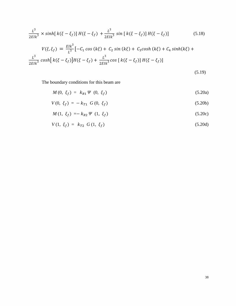
2𝐸𝐼𝑘3 𝑠𝑖𝑛 [ 𝑘(𝜉 − 𝜉𝑓)] 𝐻(𝜉 − 𝜉𝑓)] (5.18)

𝑉(𝜉, 𝜉𝑓) = 𝐸𝐼𝑘

3

𝐿3 [−𝐶1 𝑐𝑜𝑠 (𝑘𝜉) + 𝐶2 𝑠𝑖𝑛 (𝑘𝜉) + 𝐶3𝑐𝑜𝑠ℎ (𝑘𝜉) + 𝐶4 𝑠𝑖𝑛ℎ(𝑘𝜉) +

𝐿3

2𝐸𝐼𝑘3 𝑐𝑜𝑠ℎ[ 𝑘(𝜉 − 𝜉𝑓)]𝐻(𝜉 − 𝜉𝑓) +

𝐿3

2𝐸𝐼𝑘3 𝑐𝑜𝑠 [ 𝑘(𝜉 − 𝜉𝑓)] 𝐻(𝜉 − 𝜉𝑓)]

(5.19)

The boundary conditions for this beam are

M (0, 𝜉𝑓) = 𝑘𝑅1 𝛹 (0, 𝜉𝑓) (5.20a)

V (0, 𝜉𝑓) = − 𝑘𝑇1 G (0, 𝜉𝑓) (5.20b)

M (1, 𝜉𝑓) =− 𝑘𝑅2 𝛹 (1, 𝜉𝑓) (5.20c)

V (1, 𝜉𝑓) = 𝑘𝑇2 G (1, 𝜉𝑓) (5.20d)

39

Plug Eqs. (5.16) to (5.19) into boundary conditions, we have:

[ 𝑘𝑅1

𝑘𝐸𝐼

𝐿𝑘𝑅1 −

𝑘𝐸𝐼

𝐿

−𝐸𝐼𝑘3

𝐿3 𝑘𝑇1

𝐸𝐼𝑘3

𝐿3 𝑘𝑇1

−𝐸𝐼𝑘2

𝐿2𝑠𝑖𝑛(𝑘) + 𝑘𝑅2

𝑘

𝐿𝑐𝑜𝑠(𝑘) −

𝐸𝐼𝑘2

𝐿2𝑐𝑜𝑠(𝑘) − 𝑘𝑅2

𝑘

𝐿𝑠𝑖𝑛(𝑘)

𝐸𝐼𝑘2

𝐿2𝑠𝑖𝑛ℎ(𝑘)+𝑘𝑅2

𝑘

𝐿𝑐𝑜𝑠ℎ(𝑘)

𝐸𝐼𝑘2

𝐿2𝑐𝑜𝑠ℎ (𝑘) + 𝑘𝑅2

𝑘


−𝐸𝐼𝑘3

𝐿3𝑐𝑜𝑠(𝑘) − 𝑘𝑇2𝑠𝑖𝑛(𝑘)

𝐸𝐼𝑘3

𝐿3𝑠𝑖𝑛(𝑘) − 𝑘𝑇2𝑐𝑜𝑠(𝑘)

𝐸𝐼𝑘3

𝐿3𝑐𝑜𝑠ℎ(𝑘) − 𝑘𝑇2𝑠𝑖𝑛ℎ(𝑘)

𝐸𝐼𝑘3

𝐿3𝑠𝑖𝑛ℎ(𝑘) − 𝑘𝑇2𝑐𝑜𝑠ℎ(𝑘) ]

×

[ 𝐶1

𝐶2

𝐶3

𝐶4]

=

[

0

0

−𝐿

2𝑘sinh[ k(1 − 𝜉𝑓)] −

𝐿

2𝑘 sin[ k(1 − 𝜉𝑓)] −

𝑘𝑅2𝐿2

2𝐸𝐼𝑘2cosh[𝑘(1 − 𝜉𝑓)] +

𝑘𝑅2𝐿2

2𝐸𝐼𝑘2cos [𝑘(1 − 𝜉𝑓)]

−𝐿3

2𝐸𝐼𝑘3𝑠𝑖𝑛ℎ[𝑘(1 − 𝜉𝑓)] +

𝐿3

2𝐸𝐼𝑘3𝑠𝑖𝑛[𝑘(1 − 𝜉𝑓)] −

1

2cosh[𝑘(1 − 𝜉𝑓)] −

1

2cos [𝑘(1 − 𝜉𝑓)] ]

(5.21)

40

5.3 Forced Vibration of Simply Supported Euler-Bernoulli Beams

In this section, the forced vibration curve of a simply supported Euler-Bernoulli beam

under a moving delta load is derived.

For simply supported beam, the four boundary conditions are

G (0, 𝜉𝑓) = 0, G (1, 𝜉𝑓) = 0

M (0, 𝜉𝑓) = 0, M (1, 𝜉𝑓) = 0 (5.22)

Plug Eqs. (5.16) and (5.18) into boundary conditions. Eq. (5.22) can be written as:

[ 0

𝑘𝐸𝐼

𝐿0 −

𝑘𝐸𝐼

𝐿

0 1 0 1

−𝑘𝐸𝐼


𝑘𝐸𝐼


𝑘𝐸𝐼


𝑘𝐸𝐼

𝐿𝑐𝑜𝑠ℎ (𝑘)


×

[ 𝐶1

𝐶2

𝐶3

𝐶4]

=

[

0

0

−𝐿

2𝑘𝑠𝑖𝑛ℎ[ 𝑘(1 − 𝜉𝑓)] −

𝐿

2𝑘 𝑠𝑖𝑛[ 𝑘(1 − 𝜉𝑓)]

−𝐿3

2𝐸𝐼𝑘3𝑠𝑖𝑛ℎ[ 𝑘(1 − 𝜉𝑓)] +

𝐿3

2𝐸𝐼𝑘3𝑠𝑖𝑛[ 𝑘(1 − 𝜉𝑓) ] ]

(5.23)

Eq. (5.21) describes a set of four nonhomogeneous equations of a general Timoshenko

beam. When 𝑘𝑅1 and 𝑘𝑅2 equal to zero, 𝑘𝑇1 and 𝑘𝑇2 approach infinity, the general beam

becomes a simply supported beam. Eq. (5.21) can be reduced to:

41

[ 0

𝑘𝐸𝐼

𝐿0 −

𝑘𝐸𝐼

𝐿

0 1 0 1

−𝑘𝐸𝐼


𝑘𝐸𝐼


𝑘𝐸𝐼


𝑘𝐸𝐼

𝐿𝑐𝑜𝑠ℎ (𝑘)


×

[ 𝐶1

𝐶2

𝐶3

𝐶4]

=

[

0

0

−𝐿

2𝑘𝑠𝑖𝑛ℎ[ 𝑘(1 − 𝜉𝑓)] −

𝐿

2𝑘 𝑠𝑖𝑛[ 𝑘(1 − 𝜉𝑓)]

−𝐿3

2𝐸𝐼𝑘3𝑠𝑖𝑛ℎ[ 𝑘(1 − 𝜉𝑓)] +

𝐿3

2𝐸𝐼𝑘3𝑠𝑖𝑛[ 𝑘(1 − 𝜉𝑓) ] ]

(5.24)

Eq. (5.24) matches Eq. (5.23), and can be validated by a simply supported beam.

42

CHAPTER 6 Forced Vibrations of Timoshenko Beams

6.1 Deflection Curves of Forced Vibrations of Timoshenko Beams

The governing equations for forced vibration of Timoshenko beams are:

𝐸𝐼𝜕2𝜑

𝜕𝑥2 + 𝐾𝐴𝐺 (𝜕𝑦

𝜕𝑥− 𝜑) − 𝜌𝐼

𝜕2𝜑

𝜕𝑡2 = 0 (6.1)


𝜕𝑡2+ 𝐾𝐴𝐺 (

𝜕2𝑦

𝜕𝑥2−

𝜕𝜑

𝜕𝑥) = −𝑞(𝑥, 𝑡) (6.2)

where q(𝑥,t) is the applied exciting distributed load function pointing upwards. It can be

written as

𝑞(𝜉, 𝑡) = 𝑒𝑥𝑝(𝑖𝜔𝜔𝑡) 𝛿 (𝜉 − 𝜉𝑓) (6.3)

where 𝜉 is the dimensionless length x/L.

After applying separation of variable, Eqs. (6.1) and (6.2) become

𝐸𝐼𝜕4𝑦

𝜕𝑥4 + 𝜌𝐴𝜕2𝑦

𝜕𝑡2 − (𝐸𝐼𝜌

𝐾𝐺+ 𝜌𝐼)

𝜕4𝑦

𝜕𝑥2𝜕𝑡2 + 𝜌𝐼𝜌

𝐾𝐺

𝜕4𝑦

𝜕𝑡4 = 𝑞(𝑥, 𝑡) – 𝐸𝐼

𝐾𝐺𝐴

𝜕2𝑞

𝜕𝑥2 + 𝐼𝜌

𝐾𝐺𝐴 𝜕2𝑞

𝜕𝑡2 (6.4)

𝐸𝐼𝜕4𝜑

𝜕𝑥4 + 𝜌𝐴

𝜕2𝜑

𝜕𝑡2 – (

𝐸𝐼𝜌

𝐾𝐺+ 𝜌𝐼)

𝜕4𝜑

𝜕𝑥2𝜕𝑡2+ 𝜌𝐼

𝜌

𝐾𝐺

𝜕4𝜑

𝜕𝑡4=

𝜕𝑞(𝑥,𝑡)

𝜕𝑥 (6.5)

The deflection shapes for forced vibrations of a Timoshenko beam can be defined as a

Green function

𝑦(𝜉, 𝑡) = 𝑌(𝜉, 𝜉𝑓) 𝑒𝑥𝑝(𝑖𝜔𝜔𝑡) (6.6)

where 𝜉𝑓 is the point where the arbitrary force is applied at.

43

𝑌(𝜉 , 𝜉𝑓) has two components, a general solution to the homogenous equations and a

particular solution to the nonhomogeneous equations.

𝑌 (𝜉, 𝜉𝑓) = 𝑌0(𝜉) + 𝑌1(𝜉, 𝜉𝑓) 𝐻(𝜉 − 𝜉𝑓) (6.7)

From chapter 4, the homogenous solution has been given

𝑌0(𝜉) = 𝐶1 𝑐𝑜𝑠ℎ (𝑏𝛼𝜉) + 𝐶2 𝑠𝑖𝑛ℎ (𝑏𝛼𝜉) + 𝐶3 𝑐𝑜𝑠 (𝑏𝛽𝜉) + 𝐶4 𝑠𝑖𝑛 (𝑏𝛽𝜉) (6.8)

𝛹0 (𝜉) = 𝐷1 𝑠𝑖𝑛ℎ (𝑏𝛼𝜉) + 𝐷2 𝑐𝑜𝑠ℎ (𝑏𝛼𝜉) + 𝐷3 𝑠𝑖𝑛 (𝑏𝛽𝜉) + 𝐷4 𝑐𝑜𝑠 (𝑏𝛽𝜉) (6.9)

Substitute Eqs. (6.6) and (6.7) into Eq. (6.4), and omit 𝑒𝑥𝑝(𝑖𝜔𝜔𝑡) on both sides of

equation. Eq. (6.4) can be written as:

𝑑4𝑌 (𝜉,𝜉𝑓)

𝑑𝜉4+

𝐿2𝜔𝜔2𝜌(1+

𝐸

𝐺𝑘)

𝐸

𝑑2𝑌 (𝜉,𝜉𝑓)

𝑑𝜉2 +

𝐿4𝜔2(𝜌2𝜔𝜔2 𝐼

𝐺𝑘 −𝜌𝐴)

𝐸𝐼 𝑌 (𝜉, 𝜉𝑓) =

− 𝐿2

𝐺𝑘𝐴 𝑑2𝛿 (𝜉−𝜉𝑓)

𝑑𝜉2 +

𝐿4

𝐸𝐼(1 −

𝐼𝜌𝜔𝜔2

𝐺𝑘𝐴) 𝛿 (𝜉 − 𝜉𝑓) (6.10)

From section 4.1, we know

𝑏2 = 𝜌𝐴𝐿4𝜔𝜔2 / (𝐸𝐼) (6.11)

𝑟2 = 𝐼 / (𝐴𝐿2) (6.12)

𝑠2 = 𝐸𝐼 / (𝐾𝐴𝐺𝐿2) (6.13)

Eq. (6.10) can be written as

𝑌𝐼𝑉 + 𝑏2 (𝑟2 + 𝑠2) 𝑌′′ − 𝑏2 (1 − 𝑟2𝑠2𝑏2)𝑌 = (1−𝑏2𝑟2𝑠2)𝐿4

𝐸𝐼 𝛿(𝜉 − 𝜉𝑓) −

𝐿4𝑠2

𝐸𝐼 𝛿′′(𝜉 − 𝜉𝑓) (6.14)

44

The damping effect is neglected in this thesis, which may cause large errors for the

vibration curves at high frequencies. The mode shape functions derived in this chapter are just for

dimensionless frequencies b, lower than cut-off frequency (𝑏 <1

𝑟2𝑠2).

The particular solution to the nonhomogeneous Eq. (6.14) has the following format,

𝑌1(𝜉, 𝜉𝑓) = 𝑃1 𝑐𝑜𝑠ℎ[𝑏𝛼(𝜉 − 𝜉𝑓)] + 𝑃2 𝑠𝑖𝑛ℎ[𝑏𝛼(𝜉 − 𝜉𝑓)] + 𝑃3 𝑐𝑜𝑠[𝑏𝛽(𝜉 − 𝜉𝑓)]

+ 𝑃4𝑠𝑖𝑛[𝑏𝛽(𝜉 − 𝜉𝑓)] (6.15)

𝑃1 to 𝑃4 can be determined by the continuity conditions. The continuity conditions are

listed below:

𝑌 (𝜉𝑓+, 𝜉𝑓) − 𝑌 (𝜉𝑓

−, 𝜉𝑓) = 0 (6.16a)

𝛹(𝜉𝑓+, 𝜉𝑓) − 𝛹( 𝜉𝑓

−, 𝜉𝑓) = 0 (6.16b)

𝑀 (𝜉𝑓+, 𝜉𝑓) − 𝑀(𝜉𝑓

−, 𝜉𝑓) = 0 (6.16c)

𝑉(𝜉𝑓+, 𝜉𝑓) − 𝑉(𝜉𝑓

−, 𝜉𝑓) = 1 (6.16d)

Eqs. (6.1) and (6.2) can be rewritten in term of b, r, and s as:

𝑠2𝛹′′ − (1 − 𝑏2𝑟2𝑠2)𝛹 + 𝑌′/𝐿 = 0 (6.17)

𝑌′′ + 𝑏2𝑠2𝑌 − 𝐿𝛹′ =𝛿 (𝜉−𝜉𝑓)𝐿2

𝐾𝐴𝐺 (6.18)

From Eq. (6.18), 𝛹′ can be written as

𝛹′ =𝑌′′+ 𝑏2𝑠2𝑌

𝐿−

𝛿 (𝜉−𝜉𝑓)L

KAG (6.19)

45

𝛹′′ can be calculated by

𝛹′′ =𝑌′′′+ 𝑏2𝑠2𝑌′

𝐿2−

𝛿′ (𝜉−𝜉𝑓)

𝐾𝐴𝐺 (6.20)

From Eq. (6.17), we get

𝛹 = (𝑠2𝛹′′ +𝑌′

𝐿) (1 − 𝑏2𝑟2𝑠2)⁄ (6.21)

Plug Eq. (6.20) into Eq. (6.21)

𝛹 = ( 𝑠2𝑌

′′′+ 𝑏2𝑠4𝑌′

𝐿2 − 𝛿′ (𝜉−𝜉𝑓)𝑠

2

KAG+

𝑌′

𝐿) (1 − 𝑏2𝑟2𝑠2) ⁄ (6.22)

For Timoshenko beams, the moment can be calculated by

𝑀 = 𝐸𝐼𝛹′ (6.23)

Plug Eq. (6.19) in to Eq. (6.23), then M can rewritten as

𝑀 = 𝐸𝐼(𝑌′′+ 𝑏2𝑠2𝑌

𝐿−

𝛿 (𝜉−𝜉𝑓)L

KAG) (6.24)

Shear force can be obtained by

𝑉 = −𝐾𝐴𝐺(𝑌′(𝜉, 𝜉𝑓) − 𝛹(𝜉, 𝜉𝑓)) (6.25)

Plug Eq. (6.22) into Eq. (6.25), then shear force can be stated as

𝑉 = −𝐾𝐴𝐺[𝑌′ − ( 𝑠2𝑌

′′′+ 𝑏2𝑠4𝑌′

𝐿2 − 𝛿′ (𝜉−𝜉𝑓)𝑠

2

KAG+

𝑌′

𝐿) / (1 − 𝑏2𝑟2𝑠2) ] (6.26)

Plug in Eqs. (6.22), (6.24), and (6.26) to the continuity conditions. After simplifying, the

continuity conditions can be written as:

46

𝑌1(𝜉𝑓 , 𝜉𝑓) = 0 (6.27a)

(𝑏2𝑠4 + 𝐿)𝑌1′(𝜉𝑓 , 𝜉𝑓) + 𝑠2𝑌1

′′′(𝜉𝑓 , 𝜉𝑓) = 0 (6.27b)

𝑌1′′(𝜉𝑓 , 𝜉𝑓) + 𝑏2𝑠2𝑌1(𝜉𝑓, 𝜉𝑓) = 0 (6.27c)

−𝐾𝐴𝐺

𝐿2(𝑏2𝑟2−1/𝑠2)[(𝑏2𝑟2𝐿 + 𝑏2𝑠2) 𝑌1

′(𝜉𝑓 , 𝜉𝑓) − 𝑌1′′′(𝜉𝑓 , 𝜉𝑓)] = 1 (6.27d)

𝑃1 to 𝑃4 can be obtained by solving Eqs. (6.27a) to (6.27d). We get

𝑃1 = 𝑃3 = 0

𝑃2 =𝐿(1− 𝑏2𝑠2𝑟2−𝑏2𝑠2𝛼2)

𝐾𝐴𝐺𝑏3𝑠2𝛼(𝛼2+𝛽2)

𝑃4 = −𝐿(1−𝑏2𝑠2𝑟2+𝑏2𝑠2𝛽2)

𝐾𝐴𝐺𝑏3𝑠2𝛽(𝛼2+𝛽2) (6.28)

In conclusion, the vibration shapes for forced vibrations of Timoshenko beams can be

stated as

𝑌(𝜉) = 𝐶1 cosh(𝑏𝛼𝜉) + 𝐶2 sinh(𝑏𝛼𝜉) + 𝐶3 cos(𝑏𝛽𝜉 ) + 𝐶4 sin(𝑏𝛽𝜉) +

𝐿(1− 𝑏2𝑠2𝑟2−𝑏2𝑠2𝛼2)

𝐾𝐴𝐺𝑏3𝑠2𝛼(𝛼2+𝛽2)× 𝑠𝑖𝑛ℎ[𝑏𝛼(𝜉 − 𝜉𝑓)] −

𝐿(1−𝑏2𝑠2𝑟2+𝑏2𝑠2𝛽2)

𝐾𝐴𝐺𝑏3𝑠2𝛽(𝛼2+𝛽2) 𝑠𝑖𝑛[𝑏𝛽(𝜉 − 𝜉𝑓)]

(6.29)

whereand are defined as

𝛼 = √1

2[−(𝑟2 + 𝑠2) + √(𝑟2 − 𝑠2)2 +

4

𝑏2 ](6.30)

47

𝛽 = √1

2[(𝑟2 + 𝑠2) + √(𝑟2 − 𝑠2)2 +

4

𝑏2 ] (6.31)

Deflection Y, and bending slope 𝛹 can be written as

𝑌(𝜉, 𝜉𝑓) = 𝐶1 𝑐𝑜𝑠ℎ(𝑏𝛼𝜉) + 𝐶2 𝑠𝑖𝑛ℎ(𝑏𝛼𝜉) + 𝐶3 𝑐𝑜𝑠(𝑏𝛽𝜉) + 𝐶4 𝑠𝑖𝑛(𝑏𝛽𝜉) +

𝑃2 sinh[𝑏𝛼(𝜉 − 𝜉𝑓)] + 𝑃4 sin[𝑏𝛽(𝜉 − 𝜉𝑓)] (6.32)

𝛹 (𝜉, 𝜉𝑓) = 𝐷1 sinh(𝑏𝛼𝜉) + 𝐷2 cosh(𝑏𝛼𝜉) + 𝐷3 sin(𝑏𝛽𝜉) + 𝐷4 cos(𝑏𝛽𝜉) + 𝑀2 ×

𝑐𝑜𝑠ℎ[𝑏𝛼(𝜉 − 𝜉𝑓) + 𝑀4 𝑐𝑜𝑠[𝑏𝛽(𝜉 − 𝜉𝑓)] (6.33)

The coefficients from Eq. (6.32), 𝐶1 to 𝑃4 can be related with the coefficients in Eq.

(6.33), 𝐷1 to 𝑀4 by Eq. (6.5). We get

𝐶1 =𝐿𝛼

𝑏(𝛼2+𝑠2)𝐷1 𝐶2 =

𝐿𝛼

𝑏(𝛼2+𝑠2)𝐷2

𝐶3 = −𝐿𝛽

𝑏(𝛽2−𝑠2)𝐷3 𝐶4 = −

𝐿𝛽

𝑏(𝛽2−𝑠2)𝐷4

𝑃2 =𝐿𝛼

𝑏(𝛼2+𝑠2)M2 𝑃4 =

𝐿𝛽

𝑏(𝛽2−𝑠2)𝑀4

𝑀2= 𝑏(𝛼2+𝑠2)

𝐿𝛼 ×

1− 𝑏2𝑠2𝑟2−𝑏2𝑠2𝛼2

𝐾𝐴𝐺𝑏2𝑠2𝛼(𝛼2+𝛽2) 𝑀4 =

𝑏(𝛽2−𝑠2)

𝐿𝛽

1−𝑏2𝑠2𝑟2+𝑏2𝑠2𝛽2

𝐾𝐴𝐺𝑏2𝑠2𝛽(𝛼2+𝛽2) (6.34)

In summary, the bending angle 𝛹 can be written as

𝛹 (𝜉, 𝜉𝑓) = 𝐷1𝑠𝑖𝑛ℎ (𝑏𝛼𝜉) + 𝐷2 𝑐𝑜𝑠ℎ (𝑏𝛼𝜉) + 𝐷3 𝑠𝑖𝑛 (𝑏𝛽𝜉) + 𝐷4 𝑐𝑜𝑠 (𝑏𝛽𝜉) +

𝛼2+𝑠2

𝛼 ×

1− 𝑏2𝑠2𝑟2−𝑏2𝑠2𝛼2

𝐾𝐴𝐺𝑏2𝑠2𝛼(𝛼2+𝛽2)𝑐𝑜𝑠ℎ[𝑏𝛼(𝜉 − 𝜉𝑓)] −

𝛽2−𝑠2

𝛽

1−𝑏2𝑠2𝑟2+𝑏2𝑠2𝛽2

𝐾𝐴𝐺𝑏2𝑠2𝛽(𝛼2+𝛽2) 𝑐𝑜𝑠[𝑏𝛽(𝜉 − 𝜉𝑓)]

(6.35)

48

6.2 Forced Vibrations of Timoshenko Beams with Two Different Rotational Springs and

Two Different Vertical Springs

Free vibrations of the general Timoshenko beam with two different rotational springs and

two different vertical springs are discussed in section 4.2. In this section, forced vibrations of the

general Timoshenko beam are studied. To the best of my knowledge, dynamic response of the

general beam has not been published in any literature yet.

The boundary conditions are

𝑀 (0, 𝜉𝑓) = 𝑘𝑅1𝛹(0, 𝜉𝑓)

𝑉(0, 𝜉𝑓) = − 𝑘𝑇1𝑌 (0, 𝜉𝑓)

𝑀 (1, 𝜉𝑓) = −𝑘𝑅2𝛹 (1, 𝜉𝑓)

𝑉(1, 𝜉𝑓) = 𝑘𝑇2 𝑌 (1, 𝜉𝑓) (6.36)

Deflection Y, bending angle 𝛹, and moment M, can be calculated by

𝑌(𝜉, 𝜉𝑓) = 𝐿𝛼

𝑏(𝛼2+𝑠2)𝐷1𝑐𝑜𝑠ℎ (𝑏𝛼𝜉) +

𝐿𝛼

𝑏(𝛼2+𝑠2)𝐷2 𝑠𝑖𝑛ℎ (𝑏𝛼𝜉) −

𝐿𝛽

𝑏(𝛽2−𝑠2)𝐷3 𝑐𝑜𝑠 (𝑏𝛽𝜉) +

𝐿𝛽

𝑏(𝛽2−𝑠2)𝐷4 𝑠𝑖𝑛 (𝑏𝛽𝜉) +

𝐿𝛼

𝑏(𝛼2+𝑠2)𝑀2𝑠𝑖𝑛ℎ[𝑏𝛼(𝜉 − 𝜉𝑓)] +

𝐿𝛽

𝑏(𝛽2−𝑠2)𝑀4 𝑠𝑖𝑛[𝑏𝛽(𝜉 − 𝜉𝑓)]

(6.37)

𝛹(𝜉, 𝜉𝑓) = 𝐷1 𝑠𝑖𝑛ℎ (𝑏𝛼𝜉) + 𝐷2 𝑐𝑜𝑠ℎ (𝑏𝛼𝜉) + 𝐷3 𝑠𝑖𝑛 (𝑏𝛽𝜉) + 𝐷4 𝑐𝑜𝑠 (𝑏𝛽𝜉) +

𝑀2𝑐𝑜𝑠ℎ[𝑏𝛼(𝜉 − 𝜉𝑓)] + 𝑀4𝑐𝑜𝑠[𝑏𝛽(𝜉 − 𝜉𝑓)] (6.38)

𝑀(𝜉, 𝜉𝑓) = 𝐸𝐼𝑏𝛼

𝐿 𝑐𝑜𝑠ℎ (𝑏𝛼𝜉) 𝐷1 +

𝐸𝐼𝑏𝛼

𝐿 𝑠𝑖𝑛ℎ (𝑏𝛼𝜉)𝐷2 +

𝐸𝐼𝑏𝛽

𝐿 𝑐𝑜𝑠 (𝑏𝛽𝜉)𝐷3 −

𝐸𝐼𝑏𝛽

𝐿 𝑠𝑖𝑛 (𝑏𝛽𝜉)𝐷4 +

𝐸𝐼𝑏𝛼

𝐿𝑀2𝑠𝑖𝑛ℎ[𝑏𝛼(𝜉 − 𝜉𝑓)] −

𝐸𝐼𝑏𝛽

𝐿𝑀4 𝑠𝑖𝑛[𝑏𝛽(𝜉 − 𝜉𝑓)] (6.39)

49

The shear force can be calculated as

𝑉 = −𝐾𝐴𝐺(𝑌′(𝜉, 𝜉𝑓) − 𝛹(𝜉, 𝜉𝑓)) (6.40)

which can be re-written as

𝑉 = 𝐾𝐴𝐺 (𝑆2

𝛼2+𝑠2sinh(𝑏𝛼𝜉)𝐷1 +

𝑆2

𝛼2+𝑠2cosh(𝑏𝛼𝜉)𝐷2 −

𝑆2

𝛽2−𝑠2× sin(𝑏𝛽𝜉)𝐷3 −

𝑆2

𝛽2−𝑠2 cos(𝑏𝛽𝜉)𝐷4 +

𝑆2

𝛼2+𝑠2𝑀2cosh [𝑏𝛼(𝜉 −

𝜉𝑓)] −𝑆2

𝛽2−𝑠2𝑀4 𝑐𝑜𝑠[𝑏𝛽(𝜉 − 𝜉𝑓)]

(6.41)

Substitute Eqs. (6.39) to (6.41) into boundary conditions, one gets the following expression:

[


𝑏(𝛼2+𝑠2) −𝐾𝐴𝐺𝑠2

(𝛼2+𝑠2)

𝑘𝑇1𝐿𝛽

𝑏(𝛽2−𝑠2）

𝐾𝐴𝐺𝑠2

(𝛽2−𝑠2）

𝐸𝐼𝑏α

𝐿−𝑘𝑅1

𝐸𝐼𝑏β

𝐿−𝑘𝑅1

KAG𝑠2𝑏 sinh(𝑏𝛼)−𝑘𝑇2𝐿𝛼cosh (𝑏𝛼)

𝑏(𝛼2+𝑠2) 𝐾𝐴𝐺𝑠2𝑏𝑐𝑜𝑠ℎ(𝑏𝛼)−𝑘𝑇2𝐿𝛼sinh (bα)

𝑏(𝛼2+𝑠2)

−KAG𝑠2𝑏sin(bβ)+𝑘𝑇2𝐿𝛽cos (𝑏𝛼)

𝑏(𝛽2−𝑠2)

−KAG𝑠2𝑏cos(bβ)−𝑘𝑇2𝐿𝛽sin (𝑏𝛼)

𝑏(𝛽2−𝑠2)

𝐸𝐼𝑏𝛼 cosh(𝑏𝛼)+𝑘𝑅2𝐿𝑠inh(bα)

𝐿

𝐸𝐼𝑏𝛼 sinh(𝑏𝛼)+𝑘𝑅2𝐿𝑐𝑜𝑠h(bα)

𝐿

𝐸𝐼𝑏𝛽 cos(𝑏𝛼)+𝑘𝑅2𝐿𝑠in(bα)

𝐿

−𝐸𝐼𝑏𝛽 sin(𝑏𝛼)+𝑘𝑅2𝐿𝑐𝑜𝑠(bα)

𝐿 ]

×

[ 𝐷1

𝐷2

𝐷3

𝐷4]

=

[

0

0

−𝐾𝐴𝐺𝑠2

𝛼2+𝑠2 M2cosh[𝑏α(1 − 𝜉𝑓)] +

𝐾𝐴𝐺𝑠2

β2−𝑠2𝑀4 cos[𝑏β(1 − 𝜉𝑓)] +

𝐿𝛼

𝑏(𝛼2+𝑠2)𝑘𝑇2M2sinh[𝑏α(1 − 𝜉𝑓)] +

𝐿β

𝑏(β2−𝑠2)𝑀4 𝑘𝑇2sin[𝑏β(1 − 𝜉𝑓)

− 𝐸𝐼𝑏𝛼

𝐿𝑀2𝑠𝑖𝑛ℎ[𝑏𝛼(1 − 𝜉𝑓)] +

𝐸𝐼𝑏𝛽

𝐿𝑀4 𝑠𝑖𝑛[𝑏𝛽(1 − 𝜉𝑓)] −𝑘𝑅2𝑀2𝑐𝑜𝑠ℎ[𝑏𝛼(1 − 𝜉𝑓)] − 𝑘𝑅2 𝑀4𝑐𝑜𝑠[𝑏𝛽(1 − 𝜉𝑓)] ]

(6.42)

50

6.3 Forced Vibrations of Simply Supported Timoshenko Beams

Forced vibration deflection shape of a simply supported Timoshenko beam is calculated in this chapter. The boundary conditions

of a simply supported beam are

𝑌(0, 𝜉𝑓) = 0, 𝑌(1, 𝜉𝑓) = 0

𝑀 (0, 𝜉𝑓) = 0,𝑀 (1, 𝜉𝑓) = 0 (6.43)

Apply Eq. (6.37) and Eq. (6.39) into boundary conditions,

[

𝐿𝛼

𝑏(𝛼2+𝑠2)0 −

𝐿𝛽

𝑏(𝛽2−𝑠2)0

𝐸𝐼𝑏𝛼

𝐿0

𝐸𝐼𝑏𝛽

𝐿0

𝐿𝛼


𝐿𝛼


𝐿𝛽


𝐿𝛽

𝑏(𝛽2−𝑠2)𝑠𝑖𝑛 (𝑏𝛽)

𝐸𝐼𝑏𝛼

𝐿𝑐𝑜𝑠ℎ (𝑏𝛼)

𝐸𝐼𝑏𝛼

𝐿𝑠𝑖𝑛ℎ (𝑏𝛼)

𝐸𝐼𝑏𝛽

𝐿𝑐𝑜𝑠 (𝑏𝛽) −

𝐸𝐼𝑏𝛽

𝐿𝑠𝑖𝑛 (𝑏𝛽) ]

×

[ 𝐷1

𝐷2

𝐷3

𝐷4]

=

[

0

0

−𝐿𝛼

𝑏(𝛼2+𝑠2)𝑀2𝑠𝑖𝑛ℎ[𝑏𝛼(1 − 𝜉𝑓)] −

𝐿𝛽

𝑏(𝛽2−𝑠2)𝑀4𝑠𝑖𝑛 [𝑏𝛽(1 − 𝜉𝑓)]

−𝐸𝐼𝑏𝛼


𝐸𝐼𝑏𝛽

𝐿𝑀4𝑠𝑖𝑛 [𝑏𝛽(1 − 𝜉𝑓)] ]

(6.44)

51

When 𝑘𝑅1 and 𝑘𝑅2 equal to zero, 𝑘𝑇1 and 𝑘𝑇2 reach infinity, the general beam studied in section 6.2 becomes a simply

supported beam. Eq. (6.42) can be simplified to

[

𝐿𝛼

𝑏(𝛼2+𝑠2)0 −

𝐿𝛽

𝑏(𝛽2−𝑠2)0

𝐸𝐼𝑏𝛼

𝐿0

𝐸𝐼𝑏𝛽

𝐿0

𝐿𝛼


𝐿𝛼


𝐿𝛽


𝐿𝛽

𝑏(𝛽2−𝑠2)𝑠𝑖𝑛 (𝑏𝛽)

𝐸𝐼𝑏𝛼

𝐿𝑐𝑜𝑠ℎ (𝑏𝛼)

𝐸𝐼𝑏𝛼

𝐿𝑠𝑖𝑛ℎ (𝑏𝛼)

𝐸𝐼𝑏𝛽

𝐿𝑐𝑜𝑠 (𝑏𝛽) −

𝐸𝐼𝑏𝛽

𝐿𝑠𝑖𝑛 (𝑏𝛽) ]

×

[ 𝐷1

𝐷2

𝐷3

𝐷4]

=

[

0

0

−𝐿𝛼

𝑏(𝛼2+𝑠2)𝑀2𝑠𝑖𝑛ℎ[𝑏𝛼(1 − 𝜉𝑓)] −

𝐿𝛽

𝑏(𝛽2−𝑠2)𝑀4𝑠𝑖𝑛 [𝑏𝛽(1 − 𝜉𝑓)]

−𝐸𝐼𝑏𝛼


𝐸𝐼𝑏𝛽

𝐿𝑀4𝑠𝑖𝑛 [𝑏𝛽(1 − 𝜉𝑓)] ]

(6.45)

Therefore, Eq. (6.42), describing the boundary conditions of the general beam model, is verified with Eq. (6.45). The simple

beam case expressed in Eq. (6.45) is identical to that derived by Lueschen et al. (1996).

52

CHAPTER 7 Results and Discussion

7.1 Comparison of Natural Frequencies between Euler-Bernoulli Beams and Timoshenko

Beams under Free Vibrations

To verify accuracy of the numerical derivation of natural frequencies in this thesis, a

cantilever beam with a rotational spring constraint is studied using Euler-Bernoulli beam theory

and Timoshenko beam theory. The results are compared with Chen and Kiriakidis’s (2005) results.

The boundary conditions for the beam are 𝑘𝑇1 approaches infinity, 𝑘𝑅2 and 𝑘𝑇2 equal to zero.

Below is the sketch of the beam:

Figure 7.1: A Cantilever Beam with a Rotational Spring

The properties of the beam are listed in Table 7.1:

A = 15.71 𝑐𝑚2 E = 5.72× 104 𝑀𝑃𝑎 𝜌 = 1976 𝑘𝑔/𝑚3 K = 0.56

E/KG = 4.29 r = 0.012 L = 1.5 m

Table 7.1: Beam Properties for the Numerical Example in Section 7.1

Define two new variables: dimensionless rotational spring constant k^, and dimensionless

frequency γ. k^ and γ can be calculated as,

𝛾4 =𝜌𝐴𝐿4𝜔2

𝐸𝐼 (7.1)

𝑘𝑅1

𝑘𝑅1

𝑘𝑅1

𝑘𝑅1

𝑘𝑅1

𝑘𝑅1

𝑘𝑅1

𝑘𝑅1

𝑘𝑇1 = ∞

𝑘𝑇1 = ∞

𝑘𝑇1 = ∞

𝑘𝑇1 = ∞

𝑘𝑇1 = ∞

𝑘𝑇1 = ∞

𝑘𝑇1 = ∞

𝑘𝑇1 = ∞

53

𝑘^ =𝑘𝑅1𝐿

𝐸𝐼 (7.2)

Dimensionless frequency of the Euler-Bernoulli beam , and natural frequency ratio of the

Timoshenko beam to the Euler-Bernoulli beam fT/fEB, are summarized using Table 7.2. The

dimensionless frequencies of first five modes (1,5) are all smaller than the dimensionless

cut off frequency 3352.

Case 1 fT/fEB fT/fEB fT/fEB fT/fEB fT/fEB

Hinge-free

(k= 0) 3.927 0.994 7.069 0.982 10.21 0.964 13.35 0.940 16.49 0.913

k=1 1.248 0.999 4.031 0.994 7.134 0.982 10.26 0.963 13.39 0.940

k=10 1.723 0.999 4.402 0.991 7.451 0.978 10.52 0.959 13.61 0.936

k=100 1.857 0.997 4.650 0.986 7.783 0.970 10.90 0.950 14.01 0.928

Fixed-free

(k=∞) 1.875 0.997 4.694 0.986 7.855 0.969 11.00 0.947 14.14 0.924

Table 7.2: Comparison of Frequency Ratio (fT/fEB) between Timoshenko Beam and Euler-

Bernoulli Beam with Various Boundary Conditions

The results matches Chen and Kiriakidis’s (2005) results very well. Chen and Kiriakidis’s results

are tabulated in Table 7.3.

Table 7.3: Chen and Kiriakidis's Results for Comparison of Frequency Ratio (fT/fEB) between

Timoshenko Beam and Euler-Bernoulli Beam with Various Boundary Conditions

From Table 7.2, conclusions can be drawn that when dimensionless rotational spring k^

increases, the natural frequency increases. The ratio of natural frequency for the Timoshenko beam

to natural frequency for the Euler-Bernoulli beam becomes smaller at higher modes. Natural

54

frequencies at lower modes are more sensitive to boundary restraints than natural frequencies at

higher modes.

Furthermore, the frequency ratio of mode m to mode n for Euler-Bernoulli beams is

independent of the material properties and dimensions of the beam, but the frequency ratio is

dependent on the boundary constraints, 𝑘^. However, the frequency ratio of mode m to mode n for

Timoshenko beams is dependent on the materials properties, dimensions, and dimensionless

rotational spring constant 𝑘^ . For the same boundary conditions, natural frequency of the

Timoshenko beam is always less than the natural frequency of the Euler-Bernoulli beam, because

of the shear deformation and rotatory inertia effects.

In Table 7.2, the inverse slenderness ratio r is fixed at 0.012. Figure 7.2 shows the

frequency ratio fT/fEB (natural frequency of the Timoshenko beam to natural frequency of the Euler-

Bernoulli beam) with three 𝑘^ values, versus dimensionless inverse slenderness ratio r for the

first three modes. It is worth noting that the frequecy ratio fT/fEB at higher modes drops more rapidly

as r increases. The boundary restraints 𝑘^, and fT/fEB has a negative relationship.

0.9

0.92

0.94

0.96

0.98

1

0 0.01 0.02 0.03

f T/f

EB

Inverse Slenderness Ratio r

Mode 1

k^=1

k^=10

k^=100

55

Figure 7.2: Frequency Ratio (fT/fEB) between Timoshenko Beam and Euler-Bernoulli Beam

Due to Different k^, and Dimensionless Inverse Ratio r

0.88

0.9

0.92

0.94

0.96

0.98

1

0 0.005 0.01 0.015 0.02 0.025 0.03

f T/f

EB


Mode 2

k^=1

k^=10

k^=100

0.86

0.88

0.9

0.92

0.94

0.96

0.98

1

0 0.005 0.01 0.015 0.02 0.025 0.03

f T/f

EB


Mode 3

k^=1

k^=10

k^=100

56

7.2 Comparison of Mode Shapes between Euler-Bernoulli Beams and Timoshenko Beams

under Free Vibrations

7.2.1 Mode shapes Comparison of a Cantilever Beam under Free Vibration

In this section, comparison of mode shapes between an Euler-Bernoulli beam and a

Timoshenko beam is presented. The numerical example used in this section is the same as Huang’s

(1961) example. The beam properties are summarized in Table 7.4:

A =1 𝑖𝑛2 E =3× 107𝑝𝑠𝑖 𝛾 = 0.28 𝑙𝑏/𝑖𝑛3 K =2/3

E/G =8/3 r =0.02 L =14.4 in S =0.04

Table 7.4: Beam Properties for the Numerical Example in section 7.2.1

When the beam is a cantilever beam, mode shapes of the Euler-Bernoulli beam and the

Timoshenko beam have been derived in section 3.2, and section 4.3, respectively. The

dimensionless cut off frequency for the beam is 1250. The dimensionless natural frequencies of

the first five modes for the Euler-Bernoulli beam are 1.87, 4.69, 7.85, 11.00, and 14.14, which are

smaller than the cut off frequency. The dimensionless natural frequencies of the first five modes

for the Timoshenko beam are 1.87, 4.62, 7.58, 10.34, and 12.91, which are also smaller than the

cut off frequency.

57

Figure 7.3 shows the first five mode shapes for the Euler-Bernoulli beam, which can be

generated using the MATLAB program in Appendix III. Blue line represents the mode shape of

the first mode. Red line represents the mode shape of the second mode. Yellow line represents the

mode shape of the third mode. Green line represents the mode shape of the fourth mode. Black

line represents the mode shape of the mode. Each mode shape is reduced in the way that the

coefficient of hyperbolic cosine equals to 1.

Figure 7.3: First Five Mode Shapes for a Cantilever Euler-Bernoulli beam

58

Figure 7.4 sketches the first five modes shapes for the Timoshenko beam. The mode shapes

can be determined using the MATLAB program in Appendix IV. Each mode shape is reduced in

the way that the coefficient of hyperbolic cosine equals to 1.

Figure 7.4: First Five Mode Shapes of a Cantilever Timoshenko Beam

59

Figure 7.5 illustrates the comparison of the superimposed mode shape amplitude of the

first five modes for the Euler-Bernoulli beam and the Timoshenko beam.

Figure 7.5: Comparison of Superimposed Mode Shapes for a Cantilever Beam

Figure 7.5 are reproduced and compared with Huang’s (1961) plot, as shown in Figure 7.6.

Dashed line represents the superimposed mode shape for the Euler-Bernoulli beam, and continuous

line denotes the superimposed mode shape for the Timoshenko beam in Figure 7.6. It can be seen

that the results are matched well.

60

Figure 7. 6(a): Huang's (1961) Results for Superimposed Mode Shapes for a Cantilever

Beam (Dashed Line: Euler-Bernoulli Beam, Continuous Line: Timoshenko Beam)

Figure 7.6(b): Superimposed Mode Shapes for a Cantilever Beam from This Thesis

(Dashed Line: Euler-Bernoulli Beam, Continuous Line: Timoshenko Beam)

61

7.2.2 Comparison of Mode Shapes of a Beam with Two Fixed Vertical Supports and Two

Rotational Springs under Free Vibrations

In this section, mode shapes of a beam with two fixed vertical supports and two rotational

springs at both ends are presented using Euler-Bernoulli beam theory and Timoshenko beam

theory. Below is the sketch of the beam:

Figure 7.7: A Beam with Two Different Rotational Springs

Same numerical example is used as the example in section 7.2.1. Beam properties can be

found in Table 7.4. The boundary conditions of the beam are given by:

𝑘𝑇1 = 𝑘𝑇2 = ∞

𝑘𝑅1 =10𝐸𝐼

𝐿, 𝑘𝑅2 =

20𝐸𝐼

𝐿 (7.3)

The dimensionless cut off frequency for the beam equals 1250. The dimensionless natural

frequencies of the first five modes for the Euler-Bernoulli beam are 4.25, 7.14, 10.06, 12.92, and

15.71. The dimensionless natural frequencies of the first five modes for the Timoshenko beam are

4.20, 6.98, 9.67, 12.23, and 14.63. The dimensionless natural frequencies of the first five modes

for the Euler-Bernoulli beam and the Timoshenko beam are smaller than the cut off frequency.

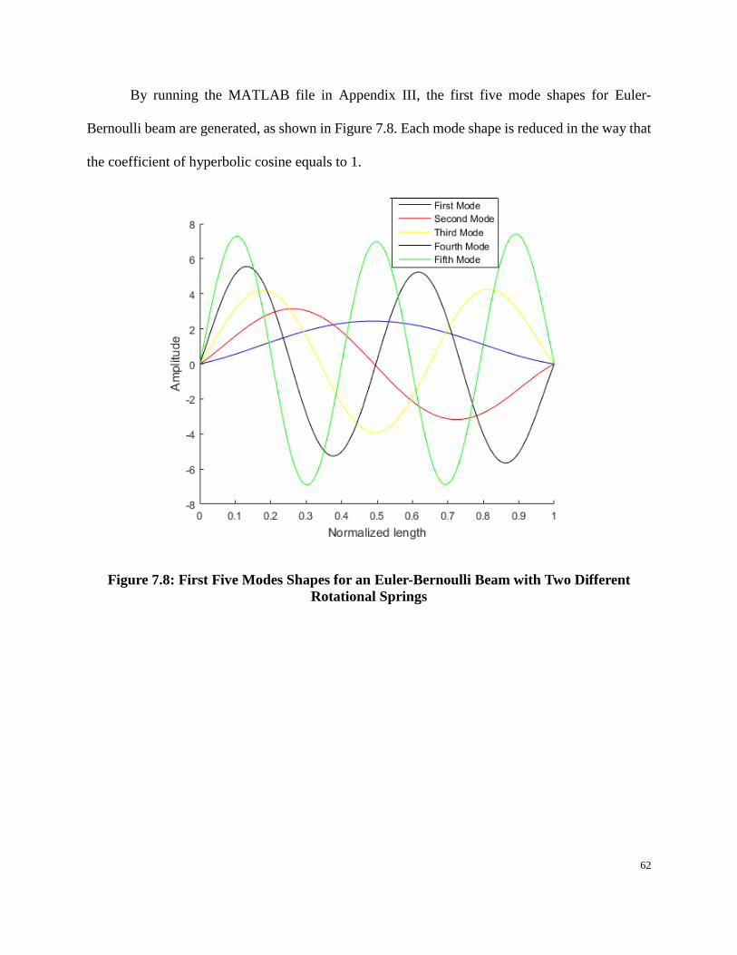
62

By running the MATLAB file in Appendix III, the first five mode shapes for Euler-

Bernoulli beam are generated, as shown in Figure 7.8. Each mode shape is reduced in the way that

the coefficient of hyperbolic cosine equals to 1.

Figure 7.8: First Five Modes Shapes for an Euler-Bernoulli Beam with Two Different

Rotational Springs

63

From Appendix IV, the first five mode shapes for the Timoshenko beam can be obtained

by inputting beam properties and boundary conditions. Each mode shape is reduced in the way

that the coefficient of hyperbolic cosine equals to 1.

Figure 7.9: First Five Modes Shapes for a Timoshenko beam with Two Different Rotational

Springs

64

Figure 7.10 illustrates the comparison of superimposed first five modes between the Euler-

Bernoulli beam and the Timoshenko beam. The red dashed line represents the superimposed mode

shape for the Euler-Bernoulli beam. The blue solid line shows the superimposed mode shape for

the Timoshenko Beam.

Figure 7.10: Comparison of Superimposed Mode Shapes for a Beam with Two Different

Rotational Springs

65

7.3 Deflection Curves Comparison of Forced Vibrations

7.3.1 Deflection Curves of a Simply Supported Beam under Forced Vibrations

In this section, comparison of deflection curves between an Euler-Bernoulli beam and a

Timoshenko beam under forced vibration of a moving delta load is presented with numerical

calculation. Using the same numerical examples as presented in Lueschen’s (1996) paper, the

beam properties are summarized in Table 7.5:

A =4 𝑖𝑛2 E =3× 107𝑝𝑠𝑖 𝜌 = 7.28 × 10−4𝑙𝑏/𝑖𝑛3 K =0.83

E/G =8/3 ʋ =0.3 L =20 in I =1.33 𝑖𝑛4

Table 7.5: Beam Properties for the Numerical Example in 7.3.1 and 7.3.2

A delta load is located at the mid-span of the simply supported beam. The cut off frequency is

25965 Hz. When the frequencies of the applied harmonic load equal to 100 Hz, 1700 Hz, 3000 Hz,

and14000 Hz, the deflection curves for the Euler-Bernoulli beam and the Timoshenko beam are

plotted in Figure 7.11

66

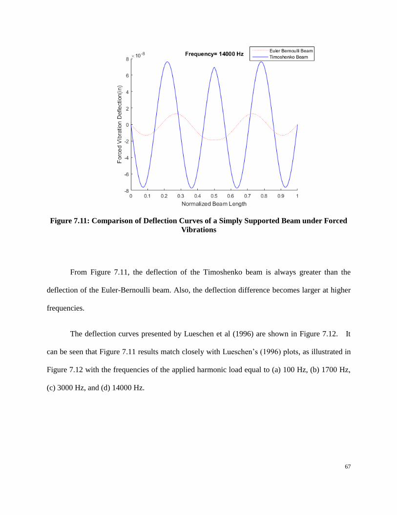
67

Figure 7.11: Comparison of Deflection Curves of a Simply Supported Beam under Forced

Vibrations

From Figure 7.11, the deflection of the Timoshenko beam is always greater than the

deflection of the Euler-Bernoulli beam. Also, the deflection difference becomes larger at higher

frequencies.

The deflection curves presented by Lueschen et al (1996) are shown in Figure 7.12. It

can be seen that Figure 7.11 results match closely with Lueschen’s (1996) plots, as illustrated in

Figure 7.12 with the frequencies of the applied harmonic load equal to (a) 100 Hz, (b) 1700 Hz,

(c) 3000 Hz, and (d) 14000 Hz.

68

Figure 7.12: Deflection Curves of a Simply Supported Beam under Forced Vibrations from

Lueschen et al. (1996), (Solid Line - Timoshenko Beam and Dotted Line - Euler Bernolli

Beam)

7.3.2 Deflection Curves of a Beam with Two Fixed Vertical Supports and Two Rotational

Springs under Forced Vibrations

In this section, deflection curves comparison of a beam with two fixed vertical supports and

two rotational springs under a moving delta load using Euler-Bernoulli beam theory and

Timoshenko beam is illustrated. The boundary conditions are shown as Figure 7.7. The

boundary conditions of the beam are given by 𝑘𝑇1 = 𝑘𝑇2 = ∞ and 𝑘𝑅1 =10𝐸𝐼

𝐿, 𝑘𝑅2 =

20𝐸𝐼

𝐿.

69

The beam properties are summarized in Table 7.5. A delta load is located at the mid-span of

the beam. The cut off frequency is 25965 Hz. When the frequencies of the applied harmonic load

equal to 100 Hz, 1700 Hz, 3000 Hz, and14000 Hz, the deflection curves for the Euler-Bernoulli

beam and the Timoshenko beam can be plotted in Figure 7.13.

70

Figure 7.13: Comparison of Deflection Curves of a Beam with Two Rotational Springs

under Forced Vibrations

71

It can be seen from the results that the deflection shapes are not symmetric when the

loading frequencies are low, because the rotational springs at two ends are different. However, the

deflection shapes tend to become symmetric at high loading frequencies. The influence of the

boundary constraints becomes smaller when the loading frequency becomes higher.

It is worth noting that when the loading frequency reaches 14000 Hz, the Euler-Bernoulli

beam and the Timoshenko beam vibrate at different modes. The natural frequency of the fifth

mode of the Euler-Bernoulli beam is 12327 Hz, and the natural frequency of the seventh mode of

the Timoshenko beam is 14592 Hz. Therefore, the Euler-Bernoulli beam vibrates at the fifth mode,

and the Timoshenko beam vibrates at the seventh mode. The deflection shapes of the beam with

harmonic excitation at 14000 Hz shown in Figure 7.11, 7.12 and 7.13 display this behavior.

72

Chapter 8 Conclusions and Recommendations

8.1 Conclusions

This study presents the derivation of natural frequencies and modes shapes of uniform

Euler-Bernoulli beams and Timoshenko beams with various boundary conditions under free

vibration using Eigenvalues and Eigenvectors. Furthermore, dynamic Green’s functions and

Fourier Transform are used to determine the deflection curve for forced vibrations of Euler-

Bernoulli beams and Timoshenko beams. A general solution for a Timoshenko beam that can be

applied to any arbitrary combinations of boundary conditions is derived, and to the best of our

knowledge, this solution is not available in the literature. In this study, the transverse vibrations of

Euler Bernoulli beams and Timoshenko beams using a general and direct beam model with two

different rotational springs and two different vertical springs at the ends are analyzed, and the

close-form solutions are presented. Numerical examples are presented to illustrate the differences

in the natural frequencies and the mode shapes between Euler-Bernoulli beams and Timoshenko

beams under free vibrations. Various boundary conditions can be achieved by assigning different

values to the four spring constants. The ratio of the natural frequency of the Timoshenko beam to

the natural frequency of the Euler-Bernoulli beams decreases at the higher modes. Natural

frequencies at the lower modes are more sensitive to the boundary restraints than the natural

frequencies at the higher modes.

73

8.2 Recommendations

The forced vibrations of uniform Euler-Bernoulli beams and Timoshenko beams are

analyzed with the assumption that internal damping and external damping are neglected. The

damping influence can cause a large error for the deflection amplitudes. The properties of the beam

are constants in this thesis, such as the Young’s modulus E, moment of inertia I, and cross section

area A. For future study, damping effects and variations of beam properties should be included. In

addition, dynamic responses of beams supported by an elastic foundation can be an interesting

topic for future study.

74

References

Abu-Hilal, M. "Forced vibration of Euler–Bernoulli beams by means of dynamic Green

functions." Journal of sound and vibration 267, no. 2 (2003): 191-207.

Azam, S. Eftekhar, M. Mofid, and R. Afghani Khoraskani. "Dynamic response of Timoshenko

beam under moving mass." Scientia Iranica 20, no. 1 (2013): 50-56.

Challis, L., and Sheard, F. "The Green of Green Functions" Physics Today 56 (2003), 41-46.

Chen, Hung-Liang Roger, and Alejandro C. Kiriakidis. "Nondestructive evaluation of ceramic

candle filter with various boundary conditions." Journal of Nondestructive Evaluation 24,

no. 2 (2005): 67-81.

Chen, Hung-Liang Roger, and Alejandro C. Kiriakidis. "Stiffness evaluation and damage detection

of ceramic candle filters." Journal of engineering mechanics126, no. 3 (2000): 308-319.

Ekwaro-Osire, S., D. H. S. Maithripala, and J. M. Berg. "A series expansion approach to

interpreting the spectra of the Timoshenko beam." Journal of sound and Vibration 240, no.

4 (2001): 667-678.

Esmailzadeh, Ebrahim, and Mehrdaad Ghorashi. "Vibration analysis of a Timoshenko beam

subjected to a travelling mass." Journal of Sound and Vibration 199, no. 4 (1997): 615-

628.

Foda, M. A., and Z. Abduljabbar. "A dynamic Green function formulation for the response of a

beam structure to a moving mass." Journal of sound and vibration 210, no. 3 (1998): 295-

306.

75

Hamada, T. R. "Dynamic analysis of a beam under a moving force: a double Laplace transform

solution." Journal of Sound and Vibration 74, no. 2 (1981): 221-233.

Huang, T. C. "The effect of rotatory inertia and of shear deformation on the frequency and normal

mode equations of uniform beams with simple end conditions." Journal of Applied

Mechanics 28, no. 4 (1961): 579-584.

Li, X. Y., X. Zhao, and Y. H. Li. "Green's functions of the forced vibration of Timoshenko beams

with damping effect." Journal of Sound and Vibration 333, no. 6 (2014): 1781-1795.

Lueschen, G. G. G., L. A. Bergman, and D. M. McFarland. "Green's functions for uniform

Timoshenko beams." Journal of Sound and Vibration 194, no. 1 (1996): 93-102.

Mackertich, Seroj. "Response of a beam to a moving mass." The Journal of the Acoustical Society

of America 92, no. 3 (1992): 1766-1769.

Majkut, Leszek. "Free and forced vibrations of Timoshenko beams described by single differential

equation." Journal of Theoretical and Applied Mechanics: 193-210.

Mehri, B. A. H. M. A. N., A. Davar, and O. Rahmani. "Dynamic Green function solution of beams

under a moving load with different boundary conditions."Scientia iranica 16, no. 3 (2009):

273-279.

Mohamad, A. S. "Tables of Green's functions for the theory of beam vibrations with general

intermediate appendages." International journal of solids and structures 31, no. 2 (1994):

257-268.

76

Radovizky, R., (2013). Simple Beam Theory.

http://web.mit.edu/16.20/homepage/7_SimpleBeamTheory/SimpleBeamTheory_files/mo

dule_7_with_solutions.pdf.

Rayleigh, John William Strutt Baron. The theory of sound. Vol. 2. Macmillan, 1896.

Roshandel, D., M. Mofid, and A. Ghannadiasl. "Modal analysis of the dynamic response of

Timoshenko beam under moving mass." Scientia Iranica. Transaction A, Civil

Engineering 22, no. 2 (2015): 331.

Ross, Timothy J., and Felix S. Wong. "Timoshenko beams with rotational end constraints."

Journal of engineering mechanics 111, no. 3 (1985): 416-430.

Timoshenko, S. P. "On the correction factor for shear of the differential equation for transverse

vibrations of prismatic bar." Philosophical Magazine 6, no. 41 (1921): 295.

Uzzal, Rajib Alam, Rama B. Bhat, and Waiz Ahmed. "Dynamic response of a beam subjected to

moving load and moving mass supported by Pasternak foundation." Shock and

Vibration 19, no. 2 (2012): 205-220.

Weaver Jr, William, Stephen P. Timoshenko, and Donovan Harold Young. Vibration problems

in engineering. John Wiley & Sons, 1990.

77

Appendixes

Appendix I Dimensionless Frequencies of Euler-Bernoulli Beams

% Input otational spring constants T1,T2 and vertical spring constants R1,R2 % K is dimensionless frequency

R1=10*E*I/L;R2=20*E*I/L; T1=9999999;T2=9999999;

clc clear k=2/3;M=4;A=1;r=0.02;E=30000;e=0.28;L=14.4;G=3*E/8; I=r*r*A*L*L; s=0.04; syms K A1=R1; A2=E*I*K/L; A3=R1; A4=-E*I*K/L; B1=-E*I*K^3/L^3; B2=T1; B3=E*I*K^3/(L^3); B4=T1; C1=-E*I*K/L*sin(K)+R2*cos(K); C2=-E*I*K/L*cos(K)-R2*sin(K); C3=E*I*K/L*sinh(K)+R2*cosh(K) C4=E*I*K/L*cosh(K)+R2*sinh(K); D1=-E*I*K^3*cos(K)/(L^3)-T2*sin(K); D2=E*I*K^3*sin(K)/(L^3)-T2*cos(K); D3=E*I*K^3*cosh(K)/(L^3)-T2*sinh(K); D4=E*I*K^3*sinh(K)/(L^3)-T2*cosh(K); H=[A1,A2,A3,A4;B1,B2,B3,B4;C1,C2,C3,C4;D1,D2,D3,D4]; Det=det(H) f1=inline(Det,'K') z=zeros(21,1); for y= 1:1:20 K=fsolve(f1,y) z(y+1)=K; end fid=fopen('N1.txt','wt'); %4.3f\n is the statistical form of the array fprintf(fid,'%4.4f\n',z)

78

Appendix II Dimensionless Frequencies of Timoshenko Beams

% Input rotational spring constants T1,T2 and vertical spring constants R1,R2

% x is dimensionless frequency

T1=999999999;T2=999999999;R1=10*E*I/L;R2=20*E*I/L;

k=2/3;M=4;A=1;r=0.02;E=30*10^6;e=0.28/(32.2/12);L=14.4;G=3*E/8; I=r*r*A*L*L; s=0.04;

syms x a=1/sqrt(2)*sqrt(-(r^2+s^2)+sqrt((r^2-s^2)^2+4/x^4)); b=1/sqrt(2)*sqrt((r^2+s^2)+sqrt((r^2-s^2)^2+4/x^4)); A1=-T1*L*(a)/(x^2*((a)^2+s^2)); A2=-E*A*s^2/(M*((a)^2+s^2)); A3=T1*L*b/(x^2*((b)^2-s^2)); A4=E*A*s^2/(M*((b)^2-s^2)); B1=E*I*x^2*(a)/L; B2=-R1; B3=E*I*x^2*(b)/L; B4=-R1; C1=(E*A*s^2*x^2*sinh(x^2*a)/M-T2*L*a*cosh(x^2*a))/(x^2*((a)^2+s^2)); C2=(E*A*s^2*x^2*cosh(x^2*a)/M-T2*L*a*sinh(x^2*a))/(x^2*((a)^2+s^2)); C3=(-E*A*s^2*x^2*sin(x^2*b)/M+T2*L*b*cos(x^2*b))/(x^2*((b)^2-s^2)); C4=(-E*A*s^2*x^2*cos(x^2*b)/M-T2*L*b*sin(x^2*b))/(x^2*((b)^2-s^2)); D1=(E*I*x^2*a*cosh(x^2*a)+R2*L*sinh(x^2*a))/L; D2=(E*I*x^2*a*sinh(x^2*a)+R2*L*cosh(x^2*a))/L; D3=(E*I*x^2*b*cos(x^2*b)+R2*L*sin(x^2*b))/L; D4=(-E*I*x^2*b*sin(x^2*b)+R2*L*cos(x^2*b))/L; H=[A1,A2,A3,A4;B1,B2,B3,B4;C1,C2,C3,C4;D1,D2,D3,D4]; Det=det(H) f1=inline(Det,'x') z=zeros(21,1); for y= 1:1:20 x=fsolve(f1,y) z(y+1)=x; end fid=fopen('N1.txt','wt'); %4.3f\n is the statistical form of the array fprintf(fid,'%4.4f\n',z)

79

Appendix III First Five Mode shapes for Euler-Bernoulli Beams

% Input the first five frequencies K % Input rotational spring constants T1,T2 and vertical spring constants R1,R2

%% Mode 1 K=2.1515; k=2/3;M=4;A=1;r=0.02;E=30000;e=0.28;L=14.4;G=3*E/8; I=r*r*A*L*L; s=0.04; R1=10*E*I/L;R2=20*E*I/L; T1=9999999;T2=9999999;

A1=R1; A2=E*I*K/L; A3=R1; A4=-E*I*K/L; B1=-E*I*K^3/L^3; B2=T1; B3=E*I*K^3/(L^3); B4=T1; C1=-E*I*K/L*sin(K)+R2*cos(K); C2=-E*I*K/L*cos(K)-R2*sin(K); C3=E*I*K/L*sinh(K)+R2*cosh(K) C4=E*I*K/L*cosh(K)+R2*sinh(K); D1=-E*I*K^3*cos(K)/(L^3)-T2*sin(K); D2=E*I*K^3*sin(K)/(L^3)-T2*cos(K); D3=E*I*K^3*cosh(K)/(L^3)-T2*sinh(K); D4=E*I*K^3*sinh(K)/(L^3)-T2*cosh(K); H=[A1,A2,A3,A4;B1,B2,B3,B4;C1,C2,C3,C4;D1,D2,D3,D4]; E11=[A1,A2,A3;B1,B2,B3;C1,C2,C3];E10=[A4;B4;C4];E01=[D1,D2,D3];E00=[D4]; MM=-inv(E11)*E10; E1=MM(1);E2=MM(2);E3=MM(3);E4=1; t=0:0.001:1; U12=E1*sin(K*t)+E2*cos(K*t)+E3*sinh(K*t)+cosh(K*t) hold on plot(t,U12,':b');

%% Mode 2 K=5.0605; k=2/3;M=4;A=1;r=0.02;E=30000;e=0.28;L=14.4;G=3*E/8; I=r*r*A*L*L; s=0.04; R1=10*E*I/L;R2=20*E*I/L; T1=9999999;T2=0;

A1=R1; A2=E*I*K/L; A3=R1; A4=-E*I*K/L; B1=-E*I*K^3/L^3; B2=T1; B3=E*I*K^3/(L^3); B4=T1;

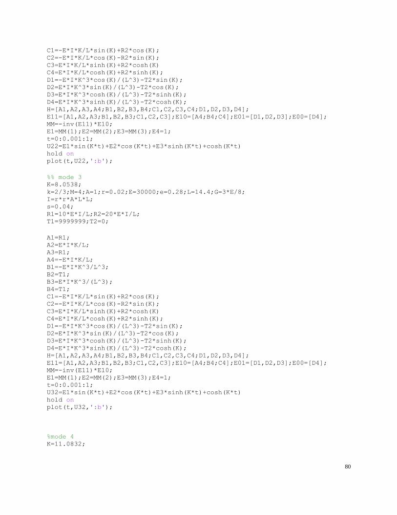
80

C1=-E*I*K/L*sin(K)+R2*cos(K); C2=-E*I*K/L*cos(K)-R2*sin(K); C3=E*I*K/L*sinh(K)+R2*cosh(K) C4=E*I*K/L*cosh(K)+R2*sinh(K); D1=-E*I*K^3*cos(K)/(L^3)-T2*sin(K); D2=E*I*K^3*sin(K)/(L^3)-T2*cos(K); D3=E*I*K^3*cosh(K)/(L^3)-T2*sinh(K); D4=E*I*K^3*sinh(K)/(L^3)-T2*cosh(K); H=[A1,A2,A3,A4;B1,B2,B3,B4;C1,C2,C3,C4;D1,D2,D3,D4]; E11=[A1,A2,A3;B1,B2,B3;C1,C2,C3];E10=[A4;B4;C4];E01=[D1,D2,D3];E00=[D4]; MM=-inv(E11)*E10; E1=MM(1);E2=MM(2);E3=MM(3);E4=1; t=0:0.001:1; U22=E1*sin(K*t)+E2*cos(K*t)+E3*sinh(K*t)+cosh(K*t) hold on plot(t,U22,':b');

%% mode 3 K=8.0538; k=2/3;M=4;A=1;r=0.02;E=30000;e=0.28;L=14.4;G=3*E/8; I=r*r*A*L*L; s=0.04; R1=10*E*I/L;R2=20*E*I/L; T1=9999999;T2=0;

A1=R1; A2=E*I*K/L; A3=R1; A4=-E*I*K/L; B1=-E*I*K^3/L^3; B2=T1; B3=E*I*K^3/(L^3); B4=T1; C1=-E*I*K/L*sin(K)+R2*cos(K); C2=-E*I*K/L*cos(K)-R2*sin(K); C3=E*I*K/L*sinh(K)+R2*cosh(K) C4=E*I*K/L*cosh(K)+R2*sinh(K); D1=-E*I*K^3*cos(K)/(L^3)-T2*sin(K); D2=E*I*K^3*sin(K)/(L^3)-T2*cos(K); D3=E*I*K^3*cosh(K)/(L^3)-T2*sinh(K); D4=E*I*K^3*sinh(K)/(L^3)-T2*cosh(K); H=[A1,A2,A3,A4;B1,B2,B3,B4;C1,C2,C3,C4;D1,D2,D3,D4]; E11=[A1,A2,A3;B1,B2,B3;C1,C2,C3];E10=[A4;B4;C4];E01=[D1,D2,D3];E00=[D4]; MM=-inv(E11)*E10; E1=MM(1);E2=MM(2);E3=MM(3);E4=1; t=0:0.001:1; U32=E1*sin(K*t)+E2*cos(K*t)+E3*sinh(K*t)+cosh(K*t) hold on plot(t,U32,':b');

%mode 4 K=11.0832;

81

k=2/3;M=4;A=1;r=0.02;E=30000;e=0.28;L=14.4;G=3*E/8; I=r*r*A*L*L; s=0.04; R1=10*E*I/L;R2=20*E*I/L; T1=9999999;T2=0;

R1=9999999; R2=0;T1=9999999;T2=0; A1=R1; A2=E*I*K/L; A3=R1; A4=-E*I*K/L; B1=-E*I*K^3/L^3; B2=T1; B3=E*I*K^3/(L^3); B4=T1; C1=-E*I*K/L*sin(K)+R2*cos(K); C2=-E*I*K/L*cos(K)-R2*sin(K); C3=E*I*K/L*sinh(K)+R2*cosh(K) C4=E*I*K/L*cosh(K)+R2*sinh(K); D1=-E*I*K^3*cos(K)/(L^3)-T2*sin(K); D2=E*I*K^3*sin(K)/(L^3)-T2*cos(K); D3=E*I*K^3*cosh(K)/(L^3)-T2*sinh(K); D4=E*I*K^3*sinh(K)/(L^3)-T2*cosh(K); H=[A1,A2,A3,A4;B1,B2,B3,B4;C1,C2,C3,C4;D1,D2,D3,D4]; E11=[A1,A2,A3;B1,B2,B3;C1,C2,C3];E10=[A4;B4;C4];E01=[D1,D2,D3];E00=[D4]; MM=-inv(E11)*E10; E1=MM(1);E2=MM(2);E3=MM(3);E4=1; t=0:0.001:1; U42=E1*sin(K*t)+E2*cos(K*t)+E3*sinh(K*t)+cosh(K*t) hold on plot(t,U42,':b'); xlabel('Normalized length') ylabel('Amplitude')

%mode 5 K=14.1371; k=2/3;M=4;A=1;r=0.02;E=30000;e=0.28;L=14.4;G=3*E/8; I=r*r*A*L*L; s=0.04; R1=10*E*I/L;R2=20*E*I/L; T1=9999999;T2=0;

A1=R1; A2=E*I*K/L; A3=R1; A4=-E*I*K/L; B1=-E*I*K^3/L^3; B2=T1; B3=E*I*K^3/(L^3); B4=T1; C1=-E*I*K/L*sin(K)+R2*cos(K); C2=-E*I*K/L*cos(K)-R2*sin(K);

82

C3=E*I*K/L*sinh(K)+R2*cosh(K) C4=E*I*K/L*cosh(K)+R2*sinh(K); D1=-E*I*K^3*cos(K)/(L^3)-T2*sin(K); D2=E*I*K^3*sin(K)/(L^3)-T2*cos(K); D3=E*I*K^3*cosh(K)/(L^3)-T2*sinh(K); D4=E*I*K^3*sinh(K)/(L^3)-T2*cosh(K); H=[A1,A2,A3,A4;B1,B2,B3,B4;C1,C2,C3,C4;D1,D2,D3,D4]; E11=[A1,A2,A3;B1,B2,B3;C1,C2,C3];E10=[A4;B4;C4];E01=[D1,D2,D3];E00=[D4]; MM=-inv(E11)*E10; E1=MM(1);E2=MM(2);E3=MM(3);E4=1; t=0:0.001:1; U52=E1*sin(K*t)+E2*cos(K*t)+E3*sinh(K*t)+cosh(K*t) hold on plot(t,U52,':b');

% super imposed mode shape U62=(U12+U22+U32+U42+U52); plot(t,U62,':r') hold off

83

Appendix IV First Five Mode shapes for Timoshenko Beams

% Input the first five frequencies x % Input rotational spring constants T1,T2 and vertical spring constants R1,R2

% Mode 1 x=1.8708; k=2/3;M=4;A=1;r=0.02;E=30000;e=0.28;L=14.4; I=r*r*A*L*L; s=0.04; a=1/sqrt(2)*sqrt(-(r^2+s^2)+sqrt((r^2-s^2)^2+4/x^4)); b=1/sqrt(2)*sqrt((r^2+s^2)+sqrt((r^2-s^2)^2+4/x^4)); A1=-T1*L*(a)/(x^2*((a)^2+s^2)); A2=-E*A*s^2/(M*((a)^2+s^2)); A3=T1*L*b/(x^2*((b)^2-s^2)); A4=E*A*s^2/(M*((b)^2-s^2)); B1=E*I*x^2*(a)/L; B2=-R1; B3=E*I*x^2*(b)/L; B4=-R1; C1=(E*A*s^2*x^2*sinh(x^2*a)/M-T2*L*a*cosh(x^2*a))/(x^2*((a)^2+s^2)); C2=(E*A*s^2*x^2*cosh(x^2*a)/M-T2*L*a*sinh(x^2*a))/(x^2*((a)^2+s^2)); C3=(-E*A*s^2*x^2*sin(x^2*b)/M+T2*L*b*cos(x^2*b))/(x^2*((b)^2-s^2)); C4=(-E*A*s^2*x^2*cos(x^2*b)/M-T2*L*b*sin(x^2*b))/(x^2*((b)^2-s^2)); D1=(E*I*x^2*a*cosh(x^2*a)+R2*L*sinh(x^2*a))/L; D2=(E*I*x^2*a*sinh(x^2*a)+R2*L*cosh(x^2*a))/L; D3=(E*I*x^2*b*cos(x^2*b)+R2*L*sin(x^2*b))/L; D4=(-E*I*x^2*b*sin(x^2*b)+R2*L*cos(x^2*b))/L; H=[A1,A2,A3,A4;B1,B2,B3,B4;C1,C2,C3,C4;D1,D2,D3,D4]; E11=[A1,A2,A3;B1,B2,B3;C1,C2,C3];E10=[A4;B4;C4];E01=[D1,D2,D3];E00=[D4]; MM=-inv(E11)*E10; E1=MM(1);E2=MM(2);E3=MM(3);E4=1; t=0:0.001:1; p=x^2 S1=(E1*L*a*cosh(p*a*t)/(p*(a^2+s^2))+E2*L*a*sinh(p*a*t)/(p*(a^2+s^2))-

E3*L*b*cos(p*b*t)/(p*(b^2-s^2))+E4*L*b*sin(p*b*t)/(p*(b^2-s^2))); Y1=(((p*(a^2+s^2))/(E1*L*a)))*S1; hold on plot(t,Y1,':b'); xlabel('Normalized length') ylabel('Amplitude')

% Mode 2 x=4.621109; k=2/3;M=4;A=1;r=0.02;E=30000;e=0.28;L=14.4; I=r*r*A*L*L; s=0.04; a=1/sqrt(2)*sqrt(-(r^2+s^2)+sqrt((r^2-s^2)^2+4/x^4)); b=1/sqrt(2)*sqrt((r^2+s^2)+sqrt((r^2-s^2)^2+4/x^4)); A1=-T1*L*(a)/(x^2*((a)^2+s^2)); A2=-E*A*s^2/(M*((a)^2+s^2)); A3=T1*L*b/(x^2*((b)^2-s^2)); A4=E*A*s^2/(M*((b)^2-s^2));

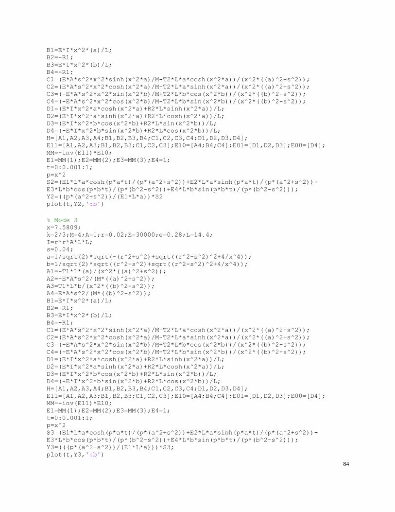
84

B1=E*I*x^2*(a)/L; B2=-R1; B3=E*I*x^2*(b)/L; B4=-R1; C1=(E*A*s^2*x^2*sinh(x^2*a)/M-T2*L*a*cosh(x^2*a))/(x^2*((a)^2+s^2)); C2=(E*A*s^2*x^2*cosh(x^2*a)/M-T2*L*a*sinh(x^2*a))/(x^2*((a)^2+s^2)); C3=(-E*A*s^2*x^2*sin(x^2*b)/M+T2*L*b*cos(x^2*b))/(x^2*((b)^2-s^2)); C4=(-E*A*s^2*x^2*cos(x^2*b)/M-T2*L*b*sin(x^2*b))/(x^2*((b)^2-s^2)); D1=(E*I*x^2*a*cosh(x^2*a)+R2*L*sinh(x^2*a))/L; D2=(E*I*x^2*a*sinh(x^2*a)+R2*L*cosh(x^2*a))/L; D3=(E*I*x^2*b*cos(x^2*b)+R2*L*sin(x^2*b))/L; D4=(-E*I*x^2*b*sin(x^2*b)+R2*L*cos(x^2*b))/L; H=[A1,A2,A3,A4;B1,B2,B3,B4;C1,C2,C3,C4;D1,D2,D3,D4]; E11=[A1,A2,A3;B1,B2,B3;C1,C2,C3];E10=[A4;B4;C4];E01=[D1,D2,D3];E00=[D4]; MM=-inv(E11)*E10; E1=MM(1);E2=MM(2);E3=MM(3);E4=1; t=0:0.001:1; p=x^2 S2=(E1*L*a*cosh(p*a*t)/(p*(a^2+s^2))+E2*L*a*sinh(p*a*t)/(p*(a^2+s^2))-

E3*L*b*cos(p*b*t)/(p*(b^2-s^2))+E4*L*b*sin(p*b*t)/(p*(b^2-s^2))); Y2=((p*(a^2+s^2))/(E1*L*a))*S2 plot(t,Y2,':b')


E3*L*b*cos(p*b*t)/(p*(b^2-s^2))+E4*L*b*sin(p*b*t)/(p*(b^2-s^2))); Y3=(((p*(a^2+s^2))/(E1*L*a)))*S3; plot(t,Y3,':b')

85



% Mode 5 x=12.909686; k=2/3;M=4;A=1;r=0.02;E=30000;e=0.28;L=14.4; I=r*r*A*L*L; s=0.04; a=1/sqrt(2)*sqrt(-(r^2+s^2)+sqrt((r^2-s^2)^2+4/x^4)); b=1/sqrt(2)*sqrt((r^2+s^2)+sqrt((r^2-s^2)^2+4/x^4)); A1=-T1*L*(a)/(x^2*((a)^2+s^2)); A2=-E*A*s^2/(M*((a)^2+s^2)); A3=T1*L*b/(x^2*((b)^2-s^2)); A4=E*A*s^2/(M*((b)^2-s^2)); B1=E*I*x^2*(a)/L; B2=-R1; B3=E*I*x^2*(b)/L; B4=-R1; C1=(E*A*s^2*x^2*sinh(x^2*a)/M-T2*L*a*cosh(x^2*a))/(x^2*((a)^2+s^2)); C2=(E*A*s^2*x^2*cosh(x^2*a)/M-T2*L*a*sinh(x^2*a))/(x^2*((a)^2+s^2)); C3=(-E*A*s^2*x^2*sin(x^2*b)/M+T2*L*b*cos(x^2*b))/(x^2*((b)^2-s^2)); C4=(-E*A*s^2*x^2*cos(x^2*b)/M-T2*L*b*sin(x^2*b))/(x^2*((b)^2-s^2)); D1=(E*I*x^2*a*cosh(x^2*a)+R2*L*sinh(x^2*a))/L; D2=(E*I*x^2*a*sinh(x^2*a)+R2*L*cosh(x^2*a))/L;

86

D3=(E*I*x^2*b*cos(x^2*b)+R2*L*sin(x^2*b))/L; D4=(-E*I*x^2*b*sin(x^2*b)+R2*L*cos(x^2*b))/L; H=[A1,A2,A3,A4;B1,B2,B3,B4;C1,C2,C3,C4;D1,D2,D3,D4];

E11=[A1,A2,A3;B1,B2,B3;C1,C2,C3];E10=[A4;B4;C4];E01=[D1,D2,D3];E00=[D4]; MM=-inv(E11)*E10; E1=MM(1);E2=MM(2);E3=MM(3);E4=1; t=0:0.001:1; p=x^2 S5=(E1*L*a*cosh(p*a*t)/(p*(a^2+s^2))+E2*L*a*sinh(p*a*t)/(p*(a^2+s^2))-


Y66=(Y1+Y2+Y3+Y4+Y5); plot(t,Y66,'-b')

87

Vita

Ye Tao was born in Jiangsu, China, on January 9, 1990, the daughter of Shijun Tao and

Hong Chen. After finishing high school in 2008, she entered West Virginia University at

Morgantown, West Virginia. She received the degree of Bachelor of Science in Civil and

Environmental Engineering in May 2013. She continued her graduate study from August 2013,

under the advisement of Dr. Roger Chen. Currently she is working at Dura-stress Inc. as a

Structural Engineer, located nearby Orlando, Florida.

Documents

Impacts of various boundary conditions on beam vibrations