Impacts and Policy Responses to a commodity price boom.

The case of Malawi

Piero Conforti, Emanuele Ferrari and Alexander Sarris♦

Paper prepared for the GTAP Twelfth Annual Conference

"Trade Integration and Sustainable Development: Looking for an Inclusive World",

Santiago, Chile, June 10-12, 2009.

Abstract: This work analyzes the medium term effects of the recent commodity price

spike in a typical Low-Income-Food-Deficit country, Malawi, as well as a set of possible

policy responses. Simulations were performed with a single-country static Computable

General Equilibrium model, based on the 2004 Malawi Social Accounting Matrix provided

by IFPRI, modified with data from the 2004 household budget survey. Results indicate that

the increase in agricultural domestic prices was mainly driven by the raise in the cost of

imported oil and chemical products. Reductions in tariff and domestic taxes, as well as

subsidies on chemicals inputs, appear capable of counteracting the terms of trade shocks to

some extent. However, tackling structural constraints, such as those affecting the size of

agricultural marketing margins, would produce wider benefits, and improve the resilience

of the economy to external shocks.

♦

Piero Conforti and Emanuele Ferrari are economists and Alexander Sarris is Director, Trade and Markets

Division, Food and Agriculture Organization of the United Nations. No senior authorship is assigned. The

opinions and judgments expressed in this paper only reflect those of the authors, while they do not reflect

those of FAO or its Member Governments.

2

1. Introduction

The instability which was recently observed in world commodity prices has raised

widespread concerns, especially for its possible consequences on weak economies such as

those of the Least Developed Countries (LDCs) and the Low-Income Food-Deficit

Countries (LIFDCs). During 2008, grain price rose by more than 60 percent, doubling the

2006 level. Rice prices almost tripled between January and May 2008. By mid-2008,

agricultural commodity prices were showing signs of stabilization, followed by a

consistent reduction. The last OECD-FAO Agriculture Outlook (OECD/FAO, 2008)

argues that prices will remain at a high level compared to the last decade, at least in the

medium term. The possibility of observing in the future more and wider spikes in

commodity prices is also mentioned frequently, with reference to long-term global issues

such as climate change and population dynamics.

Likely effects of the terms-of-trade shock in food- and oil-importing countries and LIFDCs

are an increase in the import bill, and a shift of domestic production toward more tradable

products. Such effect may have been further deepened by the depreciation of most LIFDCs

currencies with respect to the US dollar.

Despite being over, the price spike is deemed to have triggered an increase in poverty and

food insecurity, and to have contributed worsening income distribution in many developing

countries, hence reversing positive recent achievements (World Bank, 2008a; FAO,

2008a). Likely macroeconomic impacts, such as imported inflation and balance of

payments disequilibrium, amplify the vulnerability of poor countries and their ability to

cope with similar types of shock in the future. Fiscal constraints can reduce the

effectiveness of policies in alleviating negative effects on households; indeed, policies can

shape size and distribution of terms-of-trade shocks.

3

Most governments reacted quickly to the price boom, with short-run measures. Some

introduced consumer subsidies, or cuts in indirect taxation on food, and in import tariffs, to

facilitate imports, while banning exports of certain goods to enlarge domestic availability.

However easy to implement, these trade measures can bring about negative impacts in

world food markets: by restricting supply they may drive prices further up. Also, they can

contribute to tighten governments’ budgets, which often rely on tariff revenues as a key

source of finance.

The consequence of a terms-of-trade shock on the population certainly depends on the

relative share of net food sellers and buyers, but not only on that. Labour markets in

agriculture, which involve high shares of the population in low income countries, are likely

to be affected: hence better prices may represent an opportunity to improve agricultural

income. Also, higher prices affect import and export decisions, if producers manage to

perceive and react fast enough to changes. Oil and fertilizers constitute key input costs for

most agricultural and non-agricultural activities, and price changes can affect sectors to a

different extent depending on their dependence upon petroleum. Moreover, the degree of

price transmission between world and local markets determines the impact of world price

change on domestic prices. Domestic trade policies, such as tariffs and subsidies, and the

presence of high marketing margins following from infrastructural and institutional

constraints, can inhibit arbitrage and reduce the transmission of price signals

(Rapsomanikis et al., 2004).

Maize in Eastern and Southern Africa is presented as an example of poor price

transmission between world and domestic markets (FAO, 2008b). High transport costs, a

weak US dollar, consumers’ preferences for white maize -- domestic and foreign maize are

not always perfect substitutes – lack of access to markets, inadequate availability of

finance and other inputs can combine to hinder the pass trough of world prices signals in

4

the domestic markets. If this is the case, LIFDCs in the region should be protected from

world price volatility. From a partial equilibrium perspective, this could be an advantage

for consumers, at least in the short run; which can however hinder producers’ gains over

the medium term. However, the story can be more complex, given the mentioned

interactions with the factor markets, trade and macroeconomic variables, as well as due to

the structural constraints that characterize LIFDCs.

The causes of the recent price boom are multifaceted, and their analysis is beyond the

scope of this paper1. Rather, our aim is to analyze the medium-run effects of the

commodity price soar, and the possible policy responses in a typical LIFDC, like Malawi.

Understanding the impacts of a price shock on the production structure and different

population groups is important for the design of policies aimed both at counteracting such

shocks, and especially at making the economy more resilient in the medium run. In order

to accomplish this task while adding an original point of view on Malawi, we employed a

single-country static Computable General Equilibrium (CGE) model provided by IFPRI

(Lofgren et al., 2002), based on a 2004 SAM (Thurlow et al., 2008), which we modified

with data from the 2004 Second Integrated Household Survey (NSO, 2005). CGEs provide

a complete description of the economy which allows the assessment of second round

effects in all markets - including those of factors – and of distributional effects; at the same

time, macroeconomic constraints of an economy are taken into account. For this reason

CGEs have been extensively used to analyze the impact of the recent price boom (Al-Amin

et al., 2008; Arndt et al., 2008; Conforti and Sarris, 2008; Nouve and Wodon, 2008).

The price shock we considered is the change in trade unit values for Malawi – food, non-

food and petroleum -- observed between 2004 which is the base period of our dataset, and

2007. Policy experiments were then implemented on top of the price scenarios, including

1 See FAO (2008a), World Bank (2008a), von Braun et al. (2008) for a complete discussion over the causes

of soaring food prices.

5

changes in trade policies and different kinds of input subsidies, including those which have

been promoted in recent years. Given that Malawi is a landlocked country, structural

constraints play a significant role in shaping the response of the economy to external

shocks. To capture these features, our policy scenarios were simulated on two different

baselines: one reporting the observed marketing margins, and another one implying lower

marketing margins; this allowed testing the differential effects of world prices and policies

on the Malawian economy.

The remainder of the paper is organized as follows. Next section discusses a number of

facts observed in Malawi during the recent world price soar, in connection with the general

characteristics of the Malawian economy. Section 3 describes the dataset and the CGE

model employed in the analysis, while the following section illustrates the price and policy

scenarios. Section 5 analyzes the results of the simulations, as well as a set of validation

and sensitivity experiments. Finally, the last section concludes.

2. Malawi and the 2007-08 price spike

Malawi is an agricultural land-locked LIFDC country, and a net importer of oil, oil

products and fertilizers. In 2005, the last Integrated Households Survey (IHS) showed that

52 percent of the population was living below the poverty line; a proportion that was even

higher in rural areas (NSO, 2005). Poverty and productivity traps constrain economic

development, and limit the ability of the economy to grow faster. In agriculture, the

average plot size is 1.13 hectares (Benin et al., 2008), and low revenues reduce

smallholders’ chances to access fertilizer and other inputs; this is especially the case for

maize, which is the main staple crop. The reduced availability of maize is judged to pose

serious constrains to the achievement of poverty reduction and improvements in food

security (Harrigan, 2008). As it is the case in most LIFDCs, backward technologies, the

6

lack of credit towards smallholders and the persistence of poor infrastructure and high

transport costs, result in large marketing margins, which reduce the completeness and

competitiveness of markets (Dorward et al., 2008). Consequently, in the last decade value

added growth in agriculture has been erratic (NSO, 2007).

The Comprehensive Africa Agriculture Development Programme (CAADP) set a 6 percent

target for agricultural growth2. Within this framework, the Government of Malawi

committed to raise public expenditure in the sector, by financing an investment plan and an

input subsidization programme. In fact, public resources allocated to agriculture are

gaining momentum in absolute and relative terms (Benin et al., 2008). Nonetheless, public

finance constitutes a key constraint.

Since the mid 1990s, adjustment and liberalization policies have removed most subsidies

in the economy. In agriculture, this resulted in an increase of input prices (Dorward et al.,

2008) and a rapid decline of soil fertility (Harrigan, 2008). By the end of the decade the

Government decided to promote a new policy to support smallholders, involving input

subsidies, in order to reduce poverty and food insecurity. Between 1998 and 2000, the

Starter Pack Programme provided smallholders with hybrid maize and legume seeds and

fertilizers. In 2000, critiques concerning the cost of such programme led to a downsizing of

the Starter Pack, which was replaced by the Targeted Input Programme (TIP) (Harrigan,

2008). In 2005, the TIP was transformed into the Agricultural Input Subsidy Programmes

(AISP) for seasons 2005-06 and 2006-07. The broad purpose of AISP is “to improve land

and labour productivity and production of both food and cash crops by smallholder farmers

with heavy cash constraints that preclude their purchase of inputs, to promote economic

growth and reduce vulnerability to food insecurity, hunger and poverty” (Dorward et al.,

2008, p. 20). Implementation was based on the distribution of coupons allowing to

2 CAADP is part of the New Partnership for Africa’s Development (NEPAD) under the African Union (AU).

7

purchase fertilizers for maize and tobacco at a subsidized price, and to receive hybrid

maize seeds for free.

Given that 97 percent of Malawian households grow maize - either for sale or own-

consumption (NSO, 2005) -- the poverty elasticity of this product is estimated to be high,

like that of pulses, groundnuts and horticulture, and certainly higher than that of export

crops, such as tobacco, cotton, sugar and tea (Benin et al., 2008). The importance of maize

stems from its large (potential) spill-over effects on other agricultural and non agricultural

activities. Poor farmers are unable to afford fertilizers, whose limited use is among the

reasons why maize yields are low. Higher maize price could make input use more

profitable. At the same, only 10 percent of maize producers are net sellers, while 60

percent are net buyers and the majority of them are exclusively buyers (Dorward et al.,

2008). Therefore, an increase in local price of maize can directly worsen food security and

poverty conditions in many households.

In this context, the recent world price soar should have brought about mostly negative

effects. Analyses simulating changes in food prices in a short-run model of partial

equilibrium framework (Zezza et al., 2007; Ivanic and Martin, 2008), raised concerns for

poor households in rural areas, where the median welfare losses of the last quintile were

projected to be twice as large as in the first. Sarris and Rapsomanikis (2009) also found

that an increase in maize and meat prices is likely to bring about an increase in poverty and

food insecurity. However, these results were obtained by assuming that households would

not adjust to the change in relative prices, neither in terms of production or consumption.

A number of international observers claimed recently that the 2008 spike in world food

price did not affect Malawi to a significant extent (FAO, 2009; World Bank, 2008b; IMF,

2009). Still, the high prices of other key imported commodities, such as fuels and

fertilizers, must have put some pressure on the balance of payments. In fact, the

8

Government requested and received from the International Monetary Fund (IMF) a one-

year Exogenous Shocks Facility Arrangement of 77 millions of US dollars (IMF, 2009).

The impact of increased agricultural prices largely depends on the degree of integration

between domestic and world markets. Evidence for Malawi, in this respect, is mixed.

Chirwa and Zakeyo (2006) found weak price transmission, albeit showing improvement

from the mid 1990s on, following trade and price liberalization. On the contrary, Sarris and

Rapsomanikis (2009) show econometric evidence of price transmission between Malwian

and world markets, particularly with South Africa. With few exceptions, domestic markets

are found to be in a long-run equilibrium with world prices.

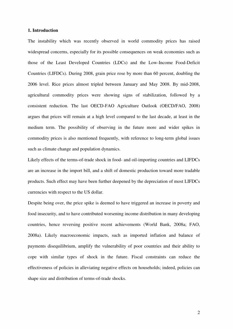
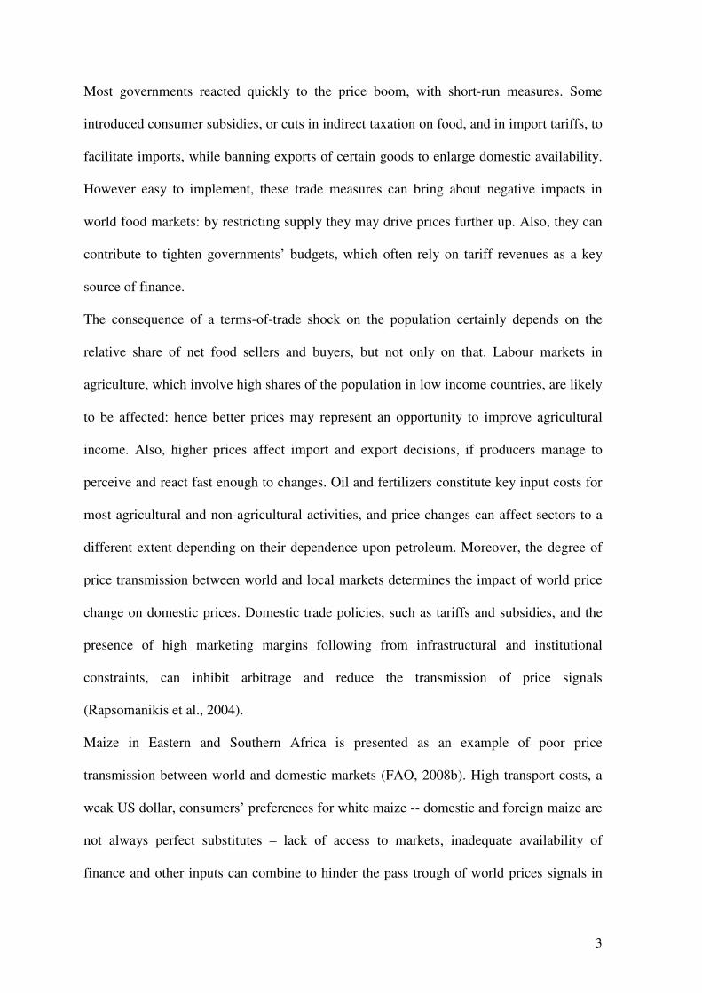
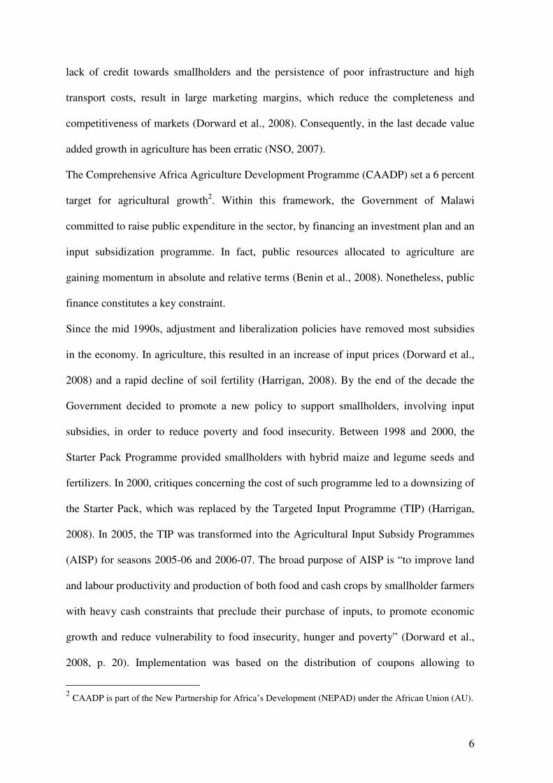
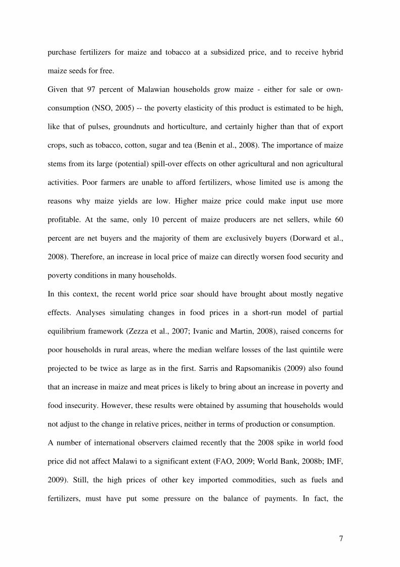
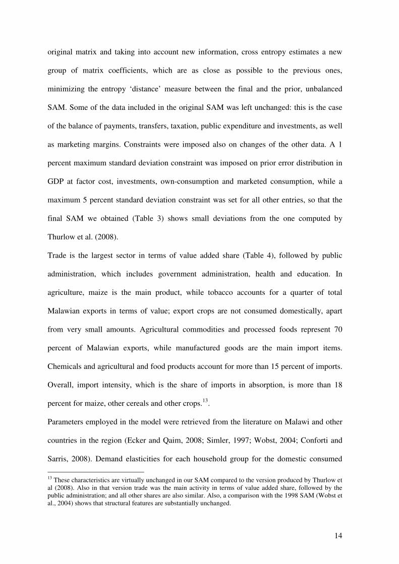
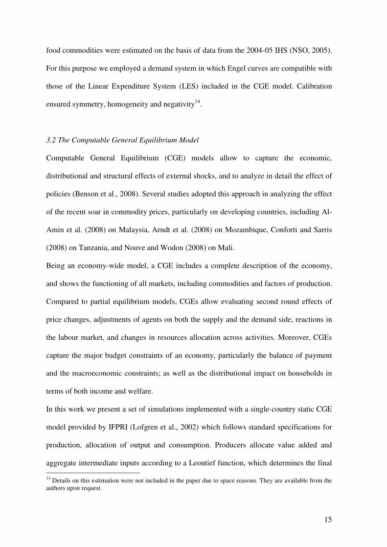
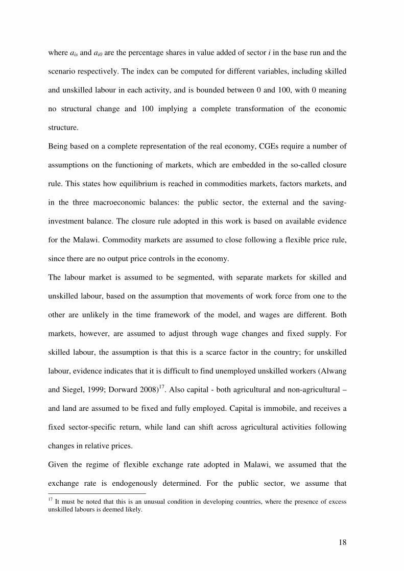
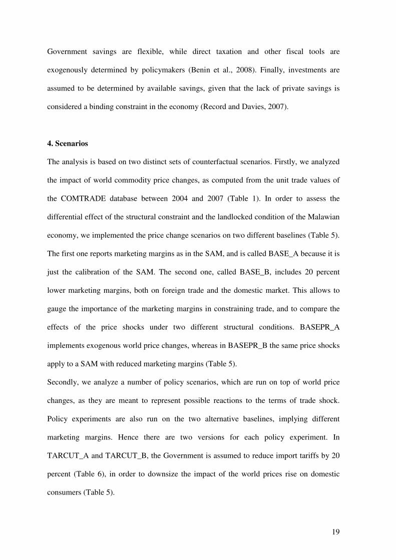
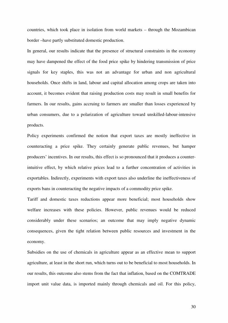
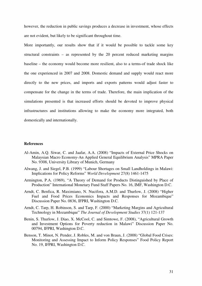
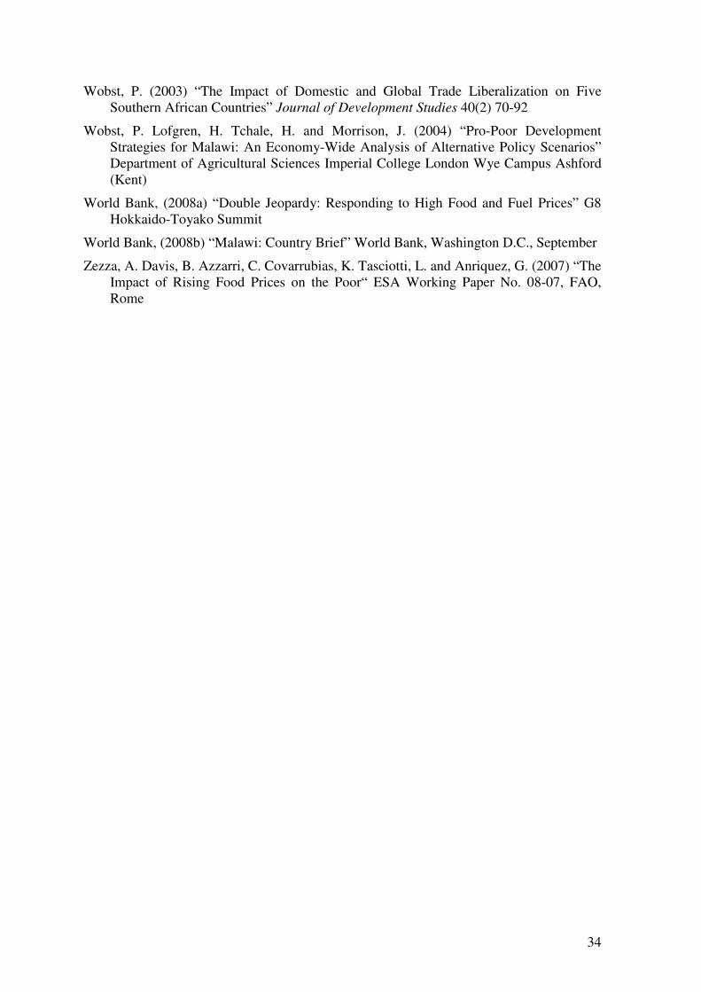
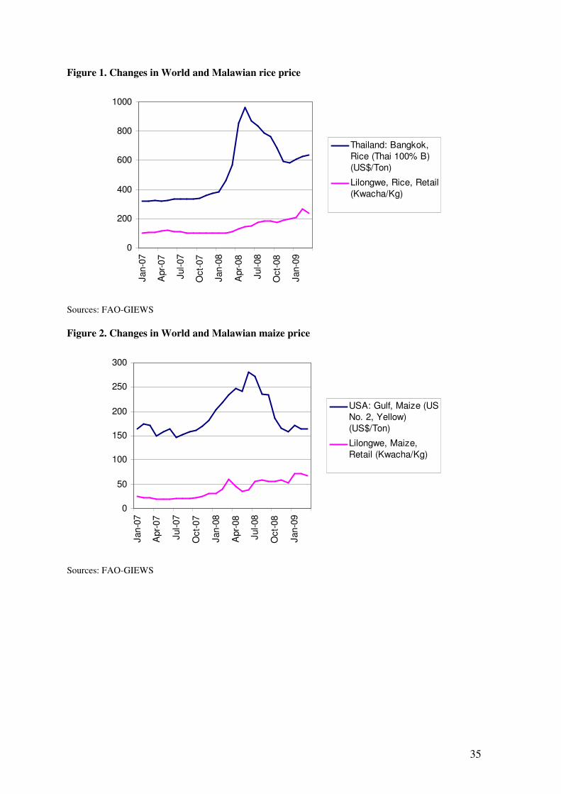
A comparison of world reference prices and retail prices in Lilongwe for maize and rice

shows a similar pattern of growth between 2006 and 2008 (Figure 1; Figure 2). It is known

that changes in retail prices in Lilongwe do not follow necessarily from changes in world

reference prices. In 2007, for instance, a bumper harvest put pressure on prices (Jayne et

al., 2008). From then on, maize prices have been increasing steadily. In August 2008, the

maize price was 186 percent higher than in the same period of 2007 (FAO, 2009), due to a

number of localized maize shortages in the 2007-08 season, as well as to the

overestimation of maize production in the Government forecasts (Jayne et al., 2008).

Based on those forecasts, the Government purchased more maize than the year before, in

an attempt to prevent a further price decrease. This resulted in increased speculation, which

contributed to determine the observed dramatic price surge. At that point, the Government

resorted to banning private trade, with the stated objective of removing speculation, and

the only authorized transactions were those operated by ADMARC3 at fixed-prices (FAO,

2009). However, informal flows of maize from neighbouring countries continued,

especially from Mozambique and Tanzania (Jayne et al., 2008). From the summer of 2008,

3 ADAMARC is the Agricultural Development and Marketing Corporation, a parastatal organization that

provides input and output markets for smallholder farmers.

9

when world cereal prices have started to fall sharply, maize prices in Lilongwe remained

about 107 percent higher than the year before (FAO, 2008c)4.

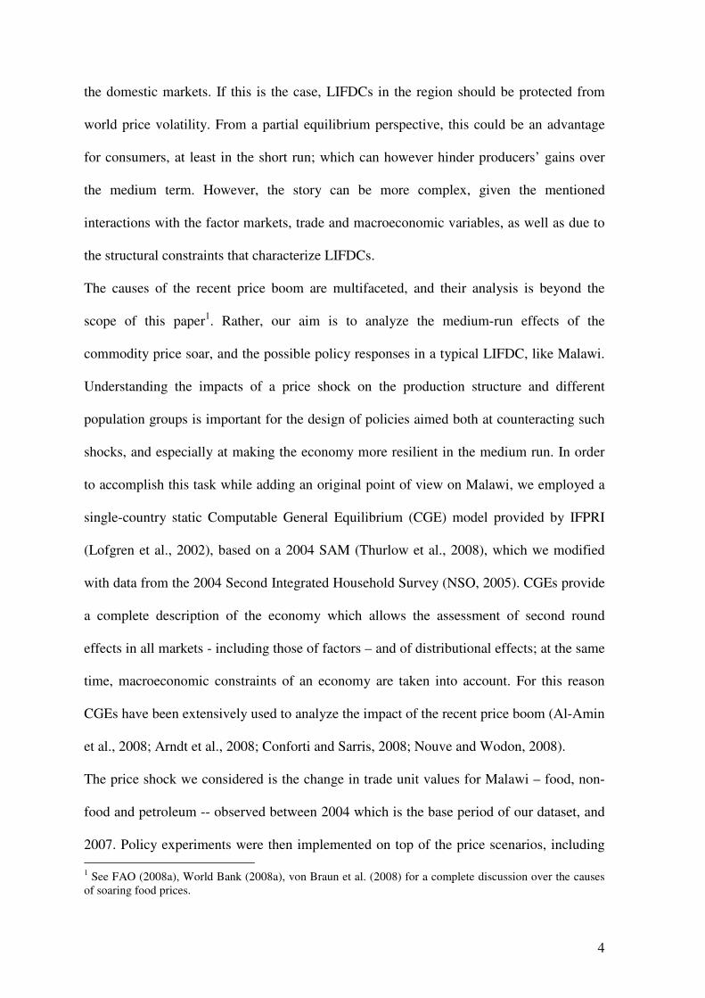
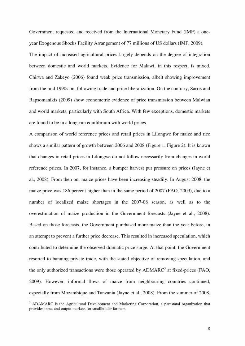
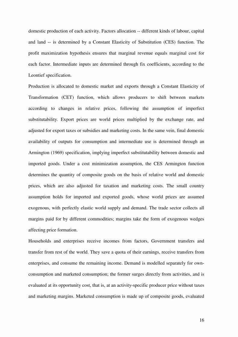
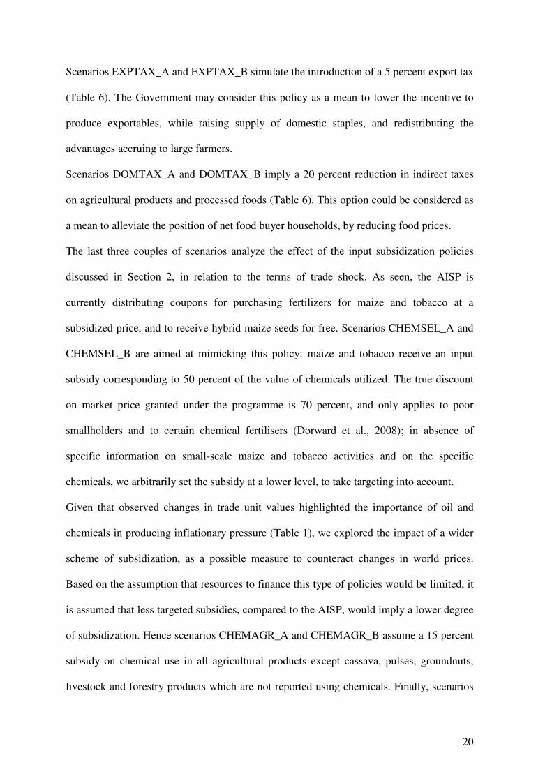
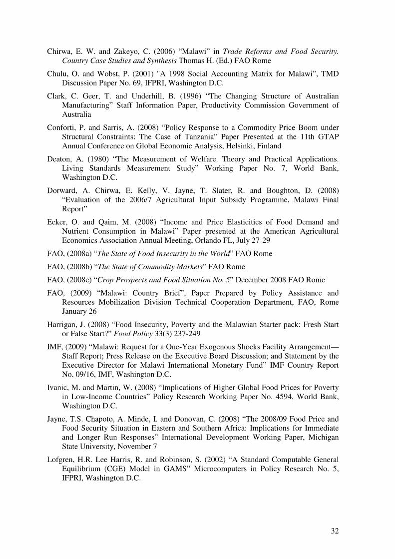
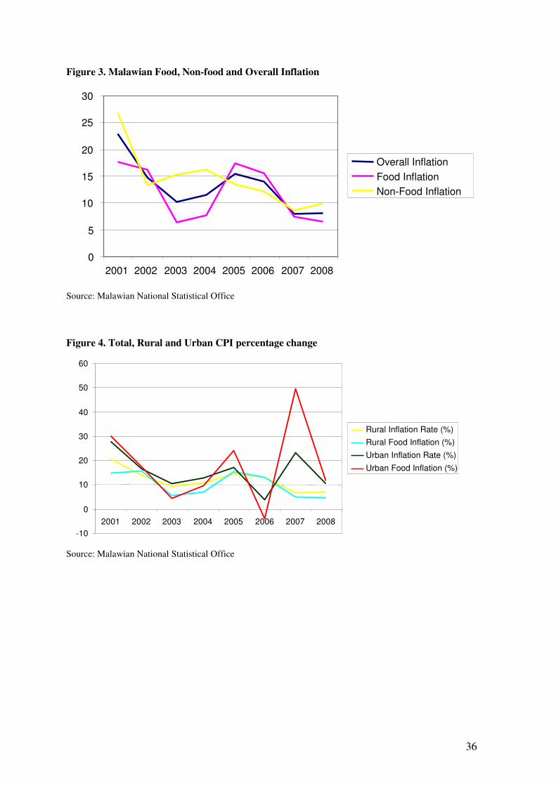
Inflation in Malawi soared between 2003 and 2005, when a drought reduced food

supplies5. A new acceleration took place from 2007 to 2008 inflation, mainly pulled by

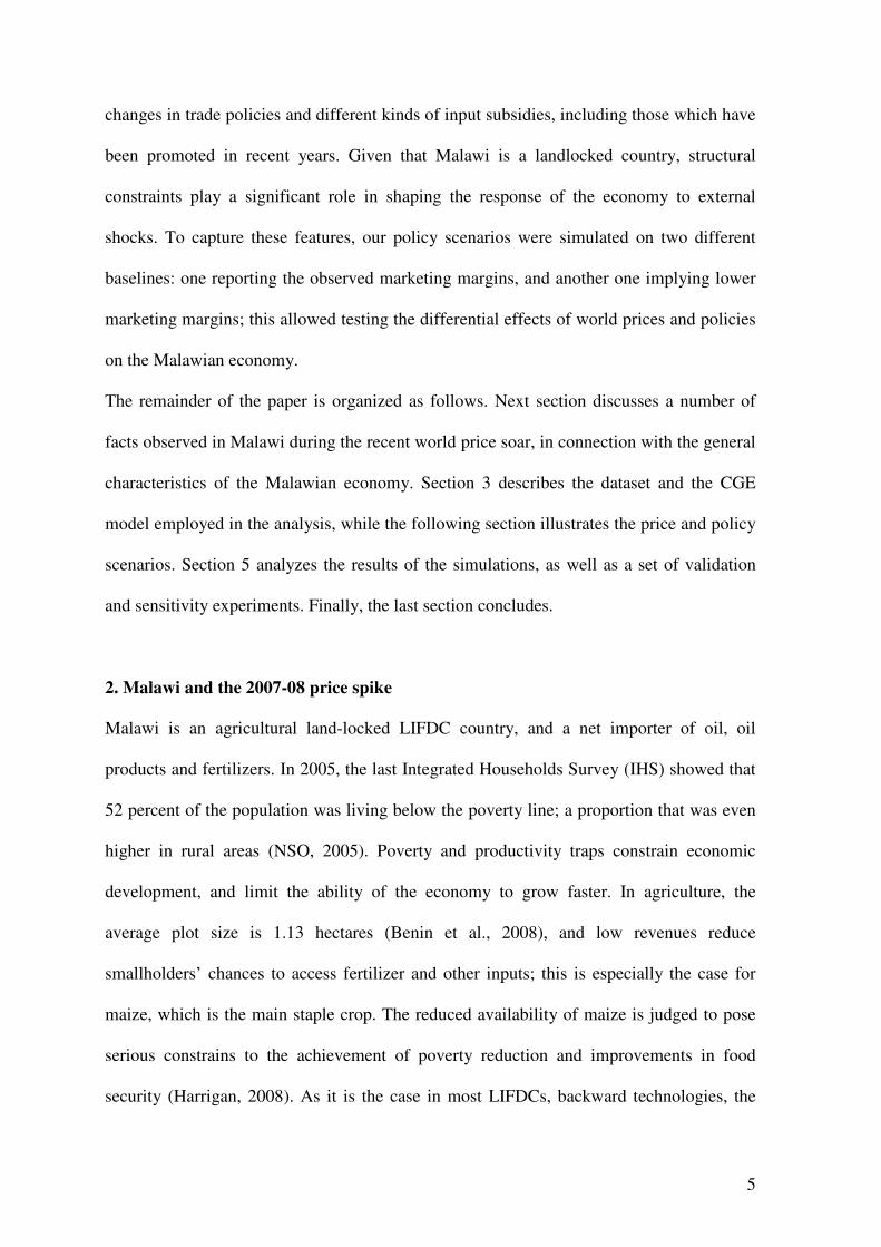
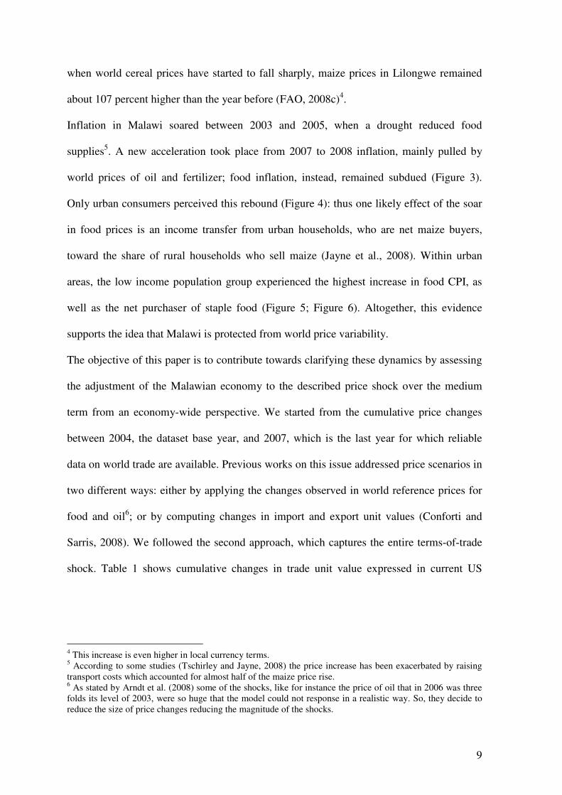
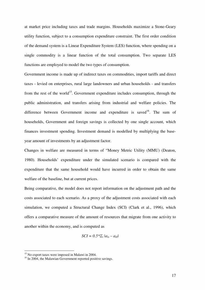
world prices of oil and fertilizer; food inflation, instead, remained subdued (Figure 3).

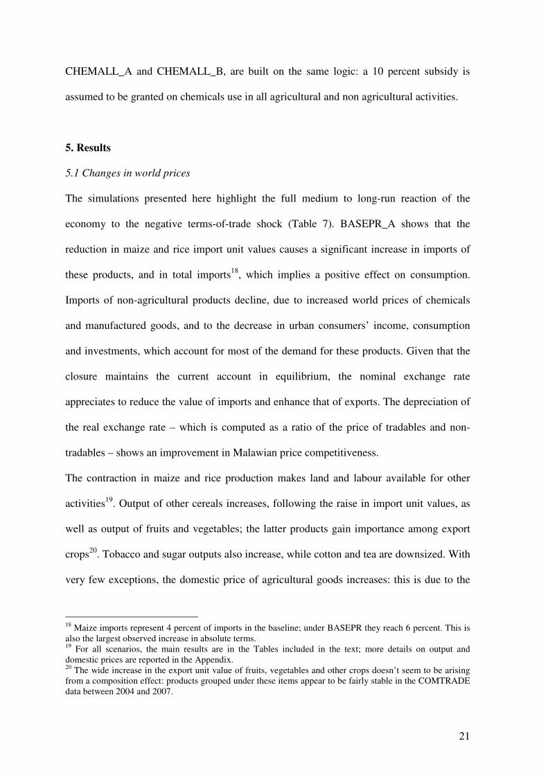
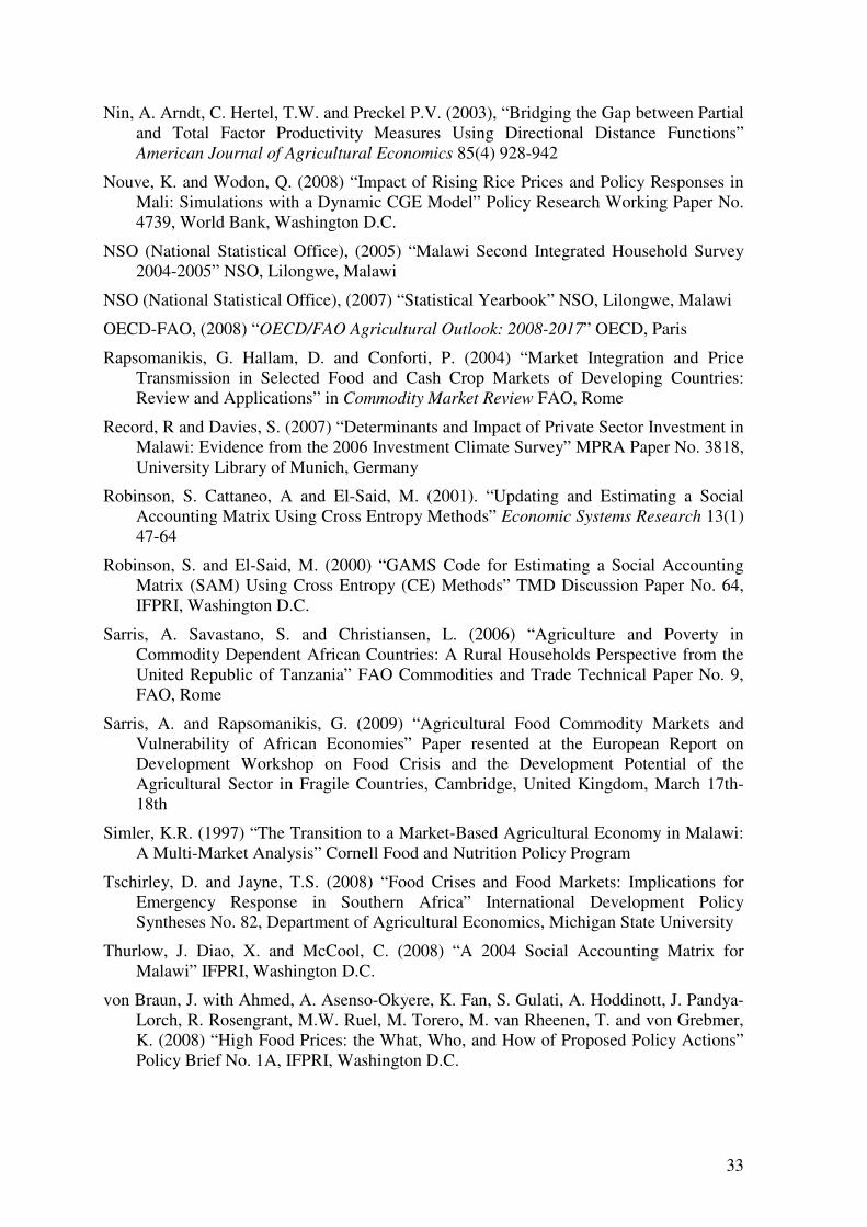
Only urban consumers perceived this rebound (Figure 4): thus one likely effect of the soar

in food prices is an income transfer from urban households, who are net maize buyers,

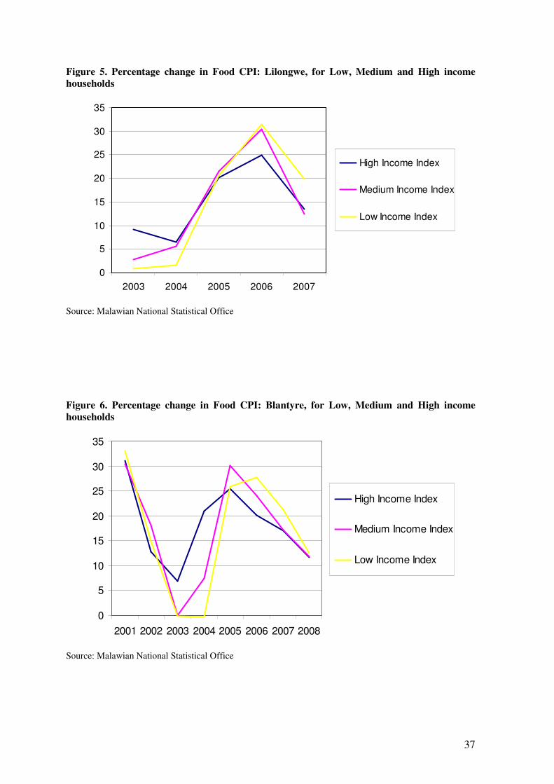
toward the share of rural households who sell maize (Jayne et al., 2008). Within urban

areas, the low income population group experienced the highest increase in food CPI, as

well as the net purchaser of staple food (Figure 5; Figure 6). Altogether, this evidence

supports the idea that Malawi is protected from world price variability.

The objective of this paper is to contribute towards clarifying these dynamics by assessing

the adjustment of the Malawian economy to the described price shock over the medium

term from an economy-wide perspective. We started from the cumulative price changes

between 2004, the dataset base year, and 2007, which is the last year for which reliable

data on world trade are available. Previous works on this issue addressed price scenarios in

two different ways: either by applying the changes observed in world reference prices for

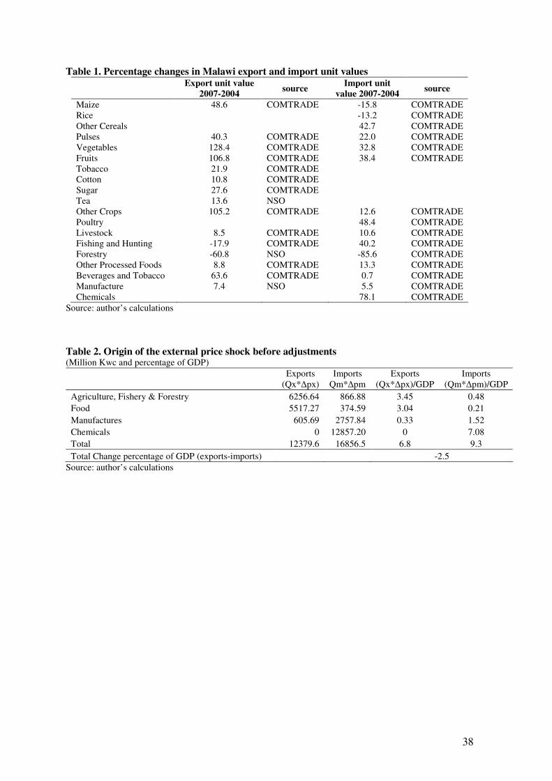
food and oil6; or by computing changes in import and export unit values (Conforti and

Sarris, 2008). We followed the second approach, which captures the entire terms-of-trade

shock. Table 1 shows cumulative changes in trade unit value expressed in current US

4 This increase is even higher in local currency terms.

5 According to some studies (Tschirley and Jayne, 2008) the price increase has been exacerbated by raising

transport costs which accounted for almost half of the maize price rise. 6 As stated by Arndt et al. (2008) some of the shocks, like for instance the price of oil that in 2006 was three

folds its level of 2003, were so huge that the model could not response in a realistic way. So, they decide to

reduce the size of price changes reducing the magnitude of the shocks.

10

dollars between 2004 and 20077. Nominal changes in US dollars were deflated with the US

GDP deflator.

Trade unit values show a considerable increase in chemicals, which includes oil and

fertilizers; a more moderate rise of import unit value of some crops, as well as a reduction

in the import unit value of maize and rice. A substantive share of maize is imported

informally from Mozambique, where 2007 brought about a bumper harvest, albeit of low

quality (Jayne et al., 2008). Apparently Mozambican farmers at the border to Malawi have

few alternative market outlets other than Malawian traders: such oligopsony power,

together with the bumper harvest, has most likely put pressure on import prices. For rice,

data from COMTRADE show that between 2004 and 2007 Malawian rice imports were

increasingly sourced from China, and less from the US. This has contributed to reduce the

import unit value, and should in itself be considered a coping strategy against raising

prices, which was implemented by several other LIFDCs even before the world price spike

of 20088.

A static measure of the terms-of-trade change that followed from the changes in trade unit

values reveals that Malawi experienced a negative shock, corresponding to 2.5 percent of

GDP (Table 2)9. The shock arises primarily from the change in the import unit value of

chemicals, which in itself correspond to 7 percent of the GDP. This is partially

7 Changes in unit values are computed from the COMTRADE database, using the SITC 2 classification at

five digits. The resulting price changes have been compared with similar data provided by the Malawian

National Statistical Office (NSO), which in most cases is consistent with the COMTRADE data. For some

product groups, however, COMTRADE data would not appear to be reliable, due to changes in the

composition of the group of products. In such cases, world price changes were retrieved from the database of

the CO.SI.MO.-AGLINK model employed by OECD and FAO in the preparation of the world agricultural

commodity outlook. For the same reason, the unit value changes for export of Manufacture, Tea and the

Forestry were retrieved directly from the Malawian NSO, valued at current US dollars. 8 This change cannot be captured by the CGE model of this work where Malawi trades internationally with a

single entity called “Rest of the World”. 9 This is computed by considering changes in imports costs and export revenues in absence of any adjustment

in the economy.

11

compensated by gains in agricultural and food exports unit values. The importance of

chemicals – both in terms of import share and intensity explains this result (Table 4).

In order to assess the medium terms reaction to this shock we need a comprehensive

dataset and a behavioural model for Malawi, which are described in the next section.

3. Data and model

3.1. The Dataset: a Modified Social Accounting Matrix for Malawi

The most recent Social Accounting Matrix (SAM) for Malawi, referred to year 2004, has

been computed by Thurlow et al. (2008); it reports thirty-six activities, of which seventeen

are part of agriculture, livestock, forestry and fisheries. Each activity produces one single

commodity, and each commodity is produced by one single activity. Given our emphasis

on agriculture, the first step in building our modified dataset, was to aggregate non-

agriculture and non-food items into ten sectors: processed food, beverage and tobacco, one

single manufacture sector, one chemical sector, and six service sectors, including trade and

public administration. Hence the SAM we used includes twenty-seven sectors, twenty-one

of which are related to agriculture and food production and processing.

The SAM reports details for nine factors of production: three types of labour, agricultural

and non-agricultural capital and four kinds of land. Elementary labour is employed only in

agriculture; unskilled labour is employed by all activities, while skilled labour is employed

only in manufacture and services10

. Land is employed only in agriculture, and is divided

into four categories: small, medium, large plots -- which are held respectively by small,

medium and large rural farmers – and urban land, which is cultivated by urban farmers.

10

Elementary labour is category 9; and unskilled labour includes categories from 8 to 4, while skilled

workers are included in category 3 of the ISCO classification -- the ILO International Standard Classification

of Occupations (http://www.ilo.org/public/english/bureau/stat/isco/index.htm).

12

Concerning institutions, the SAM takes into account the specificities of the Malawian

economy. The country has one of the highest rural population densities in Sub-Saharan

Africa, since more than 80 percent of households are rural (NSO, 2005). Hence land

availability is a constraint in agriculture, as seen from the small size of the average plot.

The SAM divides rural population into smallholders, medium scale farmers and large

owners. Small farmers are those that access less than 0.75 hectares; they produce mainly

maize, and few other crops. Medium size farmers, which are the majority of rural

households, access between 0.75 and three hectares; they show a more differentiated

cropping pattern, including maize and other crops. Large farmers are those that access

more than three hectares, and produce mainly exportables: tobacco, which is the most

important, followed by sugar, tea and cotton (Benin et al., 2008). Rural households, as

defined in the SAM, also include non-farmer households. Other households are classified

as urban and metropolitan – those living in Lilongwe and Blantyre – non-farmer, and urban

farmers households. Therefore, the SAM includes seven households. The rest of the private

sector is represented by an enterprise sector

The 2004 SAM by Thurlow et al. (2008), which we used as a starting point, does not report

own-consumption, despite this is very common, especially in rural households, but also in

urban households (NSO, 2005). Maize is the product whose share in own-consumption is

higher, but high shares of the other agricultural and food product are also directly

consumed, apart from livestock, fisheries and export crops. Therefore, we modified the

original SAM computed by Thurlow et al. (2008) to include own-consumption of

agricultural and foods based on data from the IHS (NSO, 2005)11

.

11

For each commodity the SAM reports a value of total consumption. We assumed that this would

correspond to the sum of the value of marketed consumption (Pm.Qm) and the value of own-consumption (Poc.

Qoc). We computed quantities of marketed and own-consumption from the IHS (NSO, 2005), which also

reports market price of commodities. Based on these three terms we derived the implicit unit value of own-

consumed agricultural commodities Poc. and multiplying physical quantities for it, in order to obtain a value

13

Including own-consumption in the SAM required also another modification: the inclusion

of marketing margins, which are a wedge between unit values of own-consumption and

marketed consumption. Thurlow et al. (2008) report Agricultural and Non-Agricultural

Trade as two separate distribution activities, for agricultural and non agricultural goods.

For the purpose of our work, we treated margins as costs associated with domestic sales,

exports and imports; hence we added three accounts representing margins, paid by the

commodity account in exchange for the purchase of trade and transport services. In the

modified SAM, income from these accounts accrues to a single trade sector which sums

agricultural and non-agricultural margins.

In adding the margins, we also assumed that those reported by Thurlow et al. (2008) refer

to the domestic market. The size of margins on imported and exported goods were

assumed similar to those observed in other countries of the region, as reported by Arndt et

al. (2000) for Mozambique, Wobst (2003) for the whole region; and Sarris et al. (2006) for

Tanzania. Import and export margins were assumed to be percentages of the values of

exported and imported commodities12

. The difference in the SAM generated by the

margins was subtracted from the income of the respective producers; consequently the

SAM had to be rebalanced.

To this end, we adopted the cross entropy approach (Robinson and El-Said, 2000;

Robinson et al., 2001), which allows to use all information, including errors in variables,

inequality constraints, and prior knowledge about any part of the dataset. Starting from the

of own-consumption. We assumed that also in “Food processing”, and “Beverages and Tobacco” households

would consume directly part of the production. Since these items in the SAM collect highly heterogeneous

activities, it was impossible to derive from the budget survey an implicit price; hence we applied an average

share of own-consumption. 12

For exported commodities, we assumed the margins amount to 50 percent of the exported marketed values

for agricultural goods and to 25 percent for manufacture, as in Conforti and Sarris (2008). This high level of

marketing margins come from the special position of Malawi which is land-locked, and from the analysis of

the trade flows which reveal how the majority of Malawian exports reaches countries outside the region. For

imports the same margin was set at 10 percent for maize, whose imports, instead, originate mainly

neighbouring countries; for manufactured goods the margin was assumed to be 20 percent.

14

original matrix and taking into account new information, cross entropy estimates a new

group of matrix coefficients, which are as close as possible to the previous ones,

minimizing the entropy ‘distance’ measure between the final and the prior, unbalanced

SAM. Some of the data included in the original SAM was left unchanged: this is the case

of the balance of payments, transfers, taxation, public expenditure and investments, as well

as marketing margins. Constraints were imposed also on changes of the other data. A 1

percent maximum standard deviation constraint was imposed on prior error distribution in

GDP at factor cost, investments, own-consumption and marketed consumption, while a

maximum 5 percent standard deviation constraint was set for all other entries, so that the

final SAM we obtained (Table 3) shows small deviations from the one computed by

Thurlow et al. (2008).

Trade is the largest sector in terms of value added share (Table 4), followed by public

administration, which includes government administration, health and education. In

agriculture, maize is the main product, while tobacco accounts for a quarter of total

Malawian exports in terms of value; export crops are not consumed domestically, apart

from very small amounts. Agricultural commodities and processed foods represent 70

percent of Malawian exports, while manufactured goods are the main import items.

Chemicals and agricultural and food products account for more than 15 percent of imports.

Overall, import intensity, which is the share of imports in absorption, is more than 18

percent for maize, other cereals and other crops.13

.

Parameters employed in the model were retrieved from the literature on Malawi and other

countries in the region (Ecker and Qaim, 2008; Simler, 1997; Wobst, 2004; Conforti and

Sarris, 2008). Demand elasticities for each household group for the domestic consumed

13

These characteristics are virtually unchanged in our SAM compared to the version produced by Thurlow et

al (2008). Also in that version trade was the main activity in terms of value added share, followed by the

public administration; and all other shares are also similar. Also, a comparison with the 1998 SAM (Wobst et

al., 2004) shows that structural features are substantially unchanged.

15

food commodities were estimated on the basis of data from the 2004-05 IHS (NSO, 2005).

For this purpose we employed a demand system in which Engel curves are compatible with

those of the Linear Expenditure System (LES) included in the CGE model. Calibration

ensured symmetry, homogeneity and negativity14

.

3.2 The Computable General Equilibrium Model

Computable General Equilibrium (CGE) models allow to capture the economic,

distributional and structural effects of external shocks, and to analyze in detail the effect of

policies (Benson et al., 2008). Several studies adopted this approach in analyzing the effect

of the recent soar in commodity prices, particularly on developing countries, including Al-

Amin et al. (2008) on Malaysia, Arndt et al. (2008) on Mozambique, Conforti and Sarris

(2008) on Tanzania, and Nouve and Wodon (2008) on Mali.

Being an economy-wide model, a CGE includes a complete description of the economy,

and shows the functioning of all markets, including commodities and factors of production.

Compared to partial equilibrium models, CGEs allow evaluating second round effects of

price changes, adjustments of agents on both the supply and the demand side, reactions in

the labour market, and changes in resources allocation across activities. Moreover, CGEs

capture the major budget constraints of an economy, particularly the balance of payment

and the macroeconomic constraints; as well as the distributional impact on households in

terms of both income and welfare.

In this work we present a set of simulations implemented with a single-country static CGE

model provided by IFPRI (Lofgren et al., 2002) which follows standard specifications for

production, allocation of output and consumption. Producers allocate value added and

aggregate intermediate inputs according to a Leontief function, which determines the final

14

Details on this estimation were not included in the paper due to space reasons. They are available from the

authors upon request.

16

domestic production of each activity. Factors allocation -- different kinds of labour, capital

and land -- is determined by a Constant Elasticity of Substitution (CES) function. The

profit maximization hypothesis ensures that marginal revenue equals marginal cost for

each factor. Intermediate inputs are determined through fix coefficients, according to the

Leontief specification.

Production is allocated to domestic market and exports through a Constant Elasticity of

Transformation (CET) function, which allows producers to shift between markets

according to changes in relative prices, following the assumption of imperfect

substitutability. Export prices are world prices multiplied by the exchange rate, and

adjusted for export taxes or subsidies and marketing costs. In the same vein, final domestic

availability of outputs for consumption and intermediate use is determined through an

Armington (1969) specification, implying imperfect substitutability between domestic and

imported goods. Under a cost minimization assumption, the CES Armington function

determines the quantity of composite goods on the basis of relative world and domestic

prices, which are also adjusted for taxation and marketing costs. The small country

assumption holds for imported and exported goods, whose world prices are assumed

exogenous, with perfectly elastic world supply and demand. The trade sector collects all

margins paid for by different commodities; margins take the form of exogenous wedges

affecting price formation.

Households and enterprises receive incomes from factors, Government transfers and

transfer from rest of the world. They save a quota of their earnings, receive transfers from

enterprises, and consume the remaining income. Demand is modelled separately for own-

consumption and marketed consumption; the former surges directly from activities, and is

evaluated at its opportunity cost, that is, at an activity-specific producer price without taxes

and marketing margins. Marketed consumption is made up of composite goods, evaluated

17

at market price including taxes and trade margins. Households maximize a Stone-Geary

utility function, subject to a consumption expenditure constraint. The first order condition

of the demand system is a Linear Expenditure System (LES) function, where spending on a

single commodity is a linear function of the total consumption. Two separate LES

functions are employed to model the two types of consumption.

Government income is made up of indirect taxes on commodities, import tariffs and direct

taxes - levied on enterprises, rural large landowners and urban households - and transfers

from the rest of the world15

. Government expenditure includes consumption, through the

public administration, and transfers arising from industrial and welfare policies. The

difference between Government income and expenditure is saved16

. The sum of

households, Government and foreign savings is collected by one single account, which

finances investment spending. Investment demand is modelled by multiplying the base-

year amount of investments by an adjustment factor.

Changes in welfare are measured in terms of “Money Metric Utility (MMU) (Deaton,

1980). Households’ expenditure under the simulated scenario is compared with the

expenditure that the same household would have incurred in order to obtain the same

welfare of the baseline, but at current prices.

Being comparative, the model does not report information on the adjustment path and the

costs associated to each scenario. As a proxy of the adjustment costs associated with each

simulation, we computed a Structural Change Index (SCI) (Clark et al., 1996), which

offers a comparative measure of the amount of resources that migrate from one activity to

another within the economy, and is computed as

SCI = 0.5*Σi |ais – ai0|

15

No export taxes were imposed in Malawi in 2004. 16

In 2004, the Malawian Government reported positive savings.

18

where ais and ai0 are the percentage shares in value added of sector i in the base run and the

scenario respectively. The index can be computed for different variables, including skilled

and unskilled labour in each activity, and is bounded between 0 and 100, with 0 meaning

no structural change and 100 implying a complete transformation of the economic

structure.

Being based on a complete representation of the real economy, CGEs require a number of

assumptions on the functioning of markets, which are embedded in the so-called closure

rule. This states how equilibrium is reached in commodities markets, factors markets, and

in the three macroeconomic balances: the public sector, the external and the saving-

investment balance. The closure rule adopted in this work is based on available evidence

for the Malawi. Commodity markets are assumed to close following a flexible price rule,

since there are no output price controls in the economy.

The labour market is assumed to be segmented, with separate markets for skilled and

unskilled labour, based on the assumption that movements of work force from one to the

other are unlikely in the time framework of the model, and wages are different. Both

markets, however, are assumed to adjust through wage changes and fixed supply. For

skilled labour, the assumption is that this is a scarce factor in the country; for unskilled

labour, evidence indicates that it is difficult to find unemployed unskilled workers (Alwang

and Siegel, 1999; Dorward 2008)17

. Also capital - both agricultural and non-agricultural –

and land are assumed to be fixed and fully employed. Capital is immobile, and receives a

fixed sector-specific return, while land can shift across agricultural activities following

changes in relative prices.

Given the regime of flexible exchange rate adopted in Malawi, we assumed that the

exchange rate is endogenously determined. For the public sector, we assume that

17

It must be noted that this is an unusual condition in developing countries, where the presence of excess

unskilled labours is deemed likely.

19

Government savings are flexible, while direct taxation and other fiscal tools are

exogenously determined by policymakers (Benin et al., 2008). Finally, investments are

assumed to be determined by available savings, given that the lack of private savings is

considered a binding constraint in the economy (Record and Davies, 2007).

4. Scenarios

The analysis is based on two distinct sets of counterfactual scenarios. Firstly, we analyzed

the impact of world commodity price changes, as computed from the unit trade values of

the COMTRADE database between 2004 and 2007 (Table 1). In order to assess the

differential effect of the structural constraint and the landlocked condition of the Malawian

economy, we implemented the price change scenarios on two different baselines (Table 5).

The first one reports marketing margins as in the SAM, and is called BASE_A because it is

just the calibration of the SAM. The second one, called BASE_B, includes 20 percent

lower marketing margins, both on foreign trade and the domestic market. This allows to

gauge the importance of the marketing margins in constraining trade, and to compare the

effects of the price shocks under two different structural conditions. BASEPR_A

implements exogenous world price changes, whereas in BASEPR_B the same price shocks

apply to a SAM with reduced marketing margins (Table 5).

Secondly, we analyze a number of policy scenarios, which are run on top of world price

changes, as they are meant to represent possible reactions to the terms of trade shock.

Policy experiments are also run on the two alternative baselines, implying different

marketing margins. Hence there are two versions for each policy experiment. In

TARCUT_A and TARCUT_B, the Government is assumed to reduce import tariffs by 20

percent (Table 6), in order to downsize the impact of the world prices rise on domestic

consumers (Table 5).

20

Scenarios EXPTAX_A and EXPTAX_B simulate the introduction of a 5 percent export tax

(Table 6). The Government may consider this policy as a mean to lower the incentive to

produce exportables, while raising supply of domestic staples, and redistributing the

advantages accruing to large farmers.

Scenarios DOMTAX_A and DOMTAX_B imply a 20 percent reduction in indirect taxes

on agricultural products and processed foods (Table 6). This option could be considered as

a mean to alleviate the position of net food buyer households, by reducing food prices.

The last three couples of scenarios analyze the effect of the input subsidization policies

discussed in Section 2, in relation to the terms of trade shock. As seen, the AISP is

currently distributing coupons for purchasing fertilizers for maize and tobacco at a

subsidized price, and to receive hybrid maize seeds for free. Scenarios CHEMSEL_A and

CHEMSEL_B are aimed at mimicking this policy: maize and tobacco receive an input

subsidy corresponding to 50 percent of the value of chemicals utilized. The true discount

on market price granted under the programme is 70 percent, and only applies to poor

smallholders and to certain chemical fertilisers (Dorward et al., 2008); in absence of

specific information on small-scale maize and tobacco activities and on the specific

chemicals, we arbitrarily set the subsidy at a lower level, to take targeting into account.

Given that observed changes in trade unit values highlighted the importance of oil and

chemicals in producing inflationary pressure (Table 1), we explored the impact of a wider

scheme of subsidization, as a possible measure to counteract changes in world prices.

Based on the assumption that resources to finance this type of policies would be limited, it

is assumed that less targeted subsidies, compared to the AISP, would imply a lower degree

of subsidization. Hence scenarios CHEMAGR_A and CHEMAGR_B assume a 15 percent

subsidy on chemical use in all agricultural products except cassava, pulses, groundnuts,

livestock and forestry products which are not reported using chemicals. Finally, scenarios

21

CHEMALL_A and CHEMALL_B, are built on the same logic: a 10 percent subsidy is

assumed to be granted on chemicals use in all agricultural and non agricultural activities.

5. Results

5.1 Changes in world prices

The simulations presented here highlight the full medium to long-run reaction of the

economy to the negative terms-of-trade shock (Table 7). BASEPR_A shows that the

reduction in maize and rice import unit values causes a significant increase in imports of

these products, and in total imports18

, which implies a positive effect on consumption.

Imports of non-agricultural products decline, due to increased world prices of chemicals

and manufactured goods, and to the decrease in urban consumers’ income, consumption

and investments, which account for most of the demand for these products. Given that the

closure maintains the current account in equilibrium, the nominal exchange rate

appreciates to reduce the value of imports and enhance that of exports. The depreciation of

the real exchange rate – which is computed as a ratio of the price of tradables and non-

tradables – shows an improvement in Malawian price competitiveness.

The contraction in maize and rice production makes land and labour available for other

activities19

. Output of other cereals increases, following the raise in import unit values, as

well as output of fruits and vegetables; the latter products gain importance among export

crops20

. Tobacco and sugar outputs also increase, while cotton and tea are downsized. With

very few exceptions, the domestic price of agricultural goods increases: this is due to the

18

Maize imports represent 4 percent of imports in the baseline; under BASEPR they reach 6 percent. This is

also the largest observed increase in absolute terms. 19

For all scenarios, the main results are in the Tables included in the text; more details on output and

domestic prices are reported in the Appendix. 20

The wide increase in the export unit value of fruits, vegetables and other crops doesn’t seem to be arising

from a composition effect: products grouped under these items appear to be fairly stable in the COMTRADE

data between 2004 and 2007.

22

generalized increase in oil and chemical prices employed in agriculture. Therefore, rather

than the transmission of world food prices changes to the domestic markets, the CGE

model emphasizes the impact of the increase in oil and chemical prices. Changes in the

production pattern point to a specialization of the economy in unskilled-labour-intensive

products, like cereals other than maize and rice, fruits and vegetables; while wages are

reduced in skilled employment (Table 8).

The observed decrease in Government savings (Table 7) is due to the appreciation of the

exchange rate, which reduces the value of foreign transfers; these account for almost 40

percent of Government’s revenues. The reduction in Government savings and urban

households’ income – the households with the highest propensity to save – determines a

contraction of investments.

Under BASEPR_A, all farmers, rural and urban, benefit in terms of welfare (Table 9).

Much of this stems from the increase in land and elementary labour wages. Urban

households, instead, experience a welfare reduction, due to the contraction of skilled

labour wages, and the increase in domestic prices of agriculture and foods. For urban

consumers, such price increase is not counteracted by an increase in own-consumption, as

it happens for rural households. The SAM does not report details in terms of households’

income levels; hence we cannot detect the outcome for vulnerable groups. Consistently

with what was observed in Figure 4 for inflation, households located in large urban areas

and rural landless are the hardest hit.

The SCIs is consistent with what was observed in terms of specialization towards

unskilled-labour-intensive sectors, as a reaction to the terms-of-trade shock: unskilled

labour is the factor that would be subject to the highest changes under the price change

scenarios (Table 10).

23

Compared to the standard baselines, those with reduced marketing margins (BASE_B and

BASEPR_B) show how such wedges interact with foreign trade: both on the import and

export side, the economy appears more sensitive and open to trade. The level of

consumption would consequently be higher, while Government savings would be lower

due to a higher price of the public administration services, and this would depress

investments, which depends upon the public component to a large extent. Altogether,

lowering margins appear to imply an effect similar to that of an increase in total factor

productivity: economic efficiency is improved, hence more output is produced, and there’s

an almost generalized increase in the level of factors return (Table 8). As domestic prices

become more similar to import and export prices, the former increase, in both tradable and

non-tradable activities. Consequently, also welfare is higher for all households types, and

especially for agricultural households, in both rural and urban areas, given the (assumed)

wider size of margins in agriculture (Table 9).

Compared to the calibrated baseline, under the assumption of lower marketing margins the

impact of the observed terms of trade shock would emphasize mainly the effect on imports,

which would increase by a higher percentage, starting from an already higher base (Table

7). Agricultural exports would decrease - rather than increase as with standard parameters -

due to the reduced gap between domestic and export prices which would reduce incentives

to move resources toward producing exportables. Changes in consumption would also be

smaller, while Government savings, which would start from a smaller budget surplus,

would shrink as a consequence of the increased price of public administration services.

Changes in both the nominal and the real exchange rates would be amplified, due to the

wider variation of trade, and the larger increase in the tradable to non tradable price ratio.

Altogether, lower marketing margins would make the economy more resilient to the terms

of trade shock: while foreign trade would react to a grater extent, there would be a smaller

24

shift of domestic agricultural resources towards exportables. Consequently, welfare gains

would be higher for small scale rural agriculture and for urban agriculture (Table 9).

Adjustment costs would also be smaller, as shown by the SCI for unskilled labour (Table

10).

In order to check the sensitivity of these results to the assumptions adopted in the labour

market, we run a test with an alternative closure for elementary and unskilled labour

markets, implying excess unskilled labour, with variable supply and returns are fixed at the

base level. The last column of Table 6 reports results for BASEPR_A with this

unemployment closure. Discrepancies with the standard closure are small, both in terms of

signs and in terms of the size of impacts. One minor difference which arises is the reduced

pressure on agricultural prices arising from fixed wages, which causes a slightly increase in

GDP, agricultural exports, production and consumption. The reduced price increase

translates into a diminished welfare loss for urban consumers, and an increased gain for

small, medium and urban farmers (Table 9).

5.2 Policy responses

Policy experiments are performed on the two different baselines, reporting the marketing

margins of the SAM (BASEPR_A), and the 20 percent reduced margins (BASEPR_B).

Main results are in Tables 11 and 12. A generalized reduction in import tariffs - scenarios

TARCUT_A and TARCUT_B - implies mainly a further growth of agricultural imports,

entailing small benefits from the point of view of consumption. Total imports shrink, since

the demand for manufactured products diminishes. The reduced Government savings

induce a contraction in investments which contributes to reduce supply, more than demand.

In terms of welfare, this policy shows a positive effect on all households, albeit minimal,

which would however come at a considerable cost in terms of Government savings and

25

reduced investment and consumption. The low impact of this policy in stabilizing domestic

prices is due to the low level of applied tariff rates (Table 6) and the consequent

impossibility to compensate with their reduction the high rise in international prices.

Taxing export revenues mostly imply negative consequences. An across-the-board tax on

exports, modelled in scenarios EXPTAX_A and EXPTAX_B, produces counter-intuitive

effects. By depressing returns to factors, the tax reduces output prices in most agricultural

activities. The consequent changes in factors’ allocation are such that domestic production

migrates towards exportables, overshooting the reduction in export prices brought about by

the tax. Hence exports end up increasing for most of the main agricultural exportable

products21

. At the same time, the reduction in factors’ returns associated with the export

tax depresses households’ incomes and consumption, and results in a welfare loss. The

only large gainer, under these scenarios, is the public sector, whose savings increase due to

the proceedings of the export tax. Investment, in which public investment is a large share,

increases as a consequence. Exports and imports growth brings about a significant

devaluation of both the nominal and the real exchange rates.

Scenarios DOMTAX_A and DOMTAX_B simulate a reduction in domestic taxation on

agricultural and food products. The effect of these policies on consumption shows the

expected positive sign. Tax reduction enhances consumption and production, but it also

drives up prices, especially those of agricultural products. In turn, this produces an increase

in agricultural imports, which become relatively cheaper, with the exception of processed

foods, whose price diminishes. Following the increase in consumption, welfare effects are

positive for all households, and especially for urban consumers, due to their higher reliance

on marketed production.

21

A similar outcome is found by Conforti and Sarris (2008) for Tanzania

26

Trade policy experiments show very little differentiation between the two alternative

baselines. Only those implying across-the-board tariff changes and the introduction of

export taxes in all sectors show marginally lower changes under the assumption of reduced

marketing margins.

As mentioned, the last three policy experiments deal with input subsidization in

agriculture. Those mimicking the AISP programme – CHEMSEL_A and CHEMSEL_B -

produce a decrease in the price of chemicals and in the domestic price of maize and

tobacco, which drives up production of these crops, while reducing imports (Table 11).

Following increased production of tobacco, agricultural exports increase. The reduction in

maize imports under this scenario is stronger than the increase observed in other

agricultural products, so that total agricultural imports shrink. Exports of other agricultural

and non agricultural products also diminish, so that total exports decrease. Government

revenues also decrease under this scenario, due to the reduced proceeding from import

taxes, and the reduction in public savings shrinks investment. In turn, this determines a

contraction in the demand for imported manufactured goods, which contributes to reduce

total imports. This effect holds also for the other two policy experiments implying input

subsidization; and so does also the appreciation of the real exchange, given that non-

tradables prices tend to increase relative to tradables. In terms of welfare agricultural

households benefit relatively more from this policy (Table 12), and targeting tobacco

implies benefits for large farmers. However, gains arise also for urban households,

following the reduced domestic price of maize, which is the major staple, and increased

wages for elementary labour, which contribute to increase consumption.

Differences in the results for the two baselines are minimal, and mostly related to the

public sector accounts, which however depend from the difference in the starting points.

Changes in output, domestic prices and trade are smaller under the assumption of reduced

27

marketing margins, indicating a higher resilience of the economy to the terms of trade

shock.

Smaller and less targeted input subsidies, applying to the whole agriculture - scenarios

CHEMAGR_A and CHEMAGR_B -- produce an increase in domestic prices of maize and

other staples, such as cassava and pulses, as well as groundnuts; and a price decrease for

exportables, such as tobacco. As a result, imports of staples become relatively cheap, and

domestic production decreases, partly crowded out by imports. On the export side, the

generalized subsidy results in an expansion of exports, driven by tobacco (Table 11). Non

agricultural imports, at the same time, increase. Households’ consumption still increases,

as well as welfare (Table 12): despite gains are concentrated in agricultural households,

some positive effects arise also for non-agricultural and urban households.

Finally, scenarios CHEMALL_A and CHEMALL_B – assuming a 10 percent subsidy on

all activities employing chemicals and oil – are not too different from those of the previous

scenarios. The generalized subsidy still determines an increase in the domestic price of

maize, cassava, groundnuts and vegetables; and a reduction in those of agricultural

exportables and manufactured goods. On the exports side, non agricultural products are

hindered, while export crops benefit, with the exception of tobacco. The comparison of all

policies under the two different baselines chosen shows very similar effects on the

economy.

5.3 Sensitivity and model validation

A number of tests where run on the results with the aim of understanding their degree of

robustness. Firstly, sensitivity was assessed with respect to the value of key parameters: we

repeated the simulations described in the last section with different values for the constant

elasticity of transformation (CET), that allocates production between domestic markets and

28

exports; for the Armington constant elasticity of substitution (CES), that controls

consumers’ preference between domestically produced and imported goods; and for the

constant elasticity of substitution (CES) at the bottom nest of the production function,

which rules the substitution among factors. Besides sensitivity, changes in these

parameters can also be interpreted as counterfactual scenarios in which the economy is

assumed to be more integrated in world markets, and more rapidly reacting to foreign price

signals.

Trade elasticities were augmented by 50 percent, while production parameters were

doubled. These tests were performed on all activities, as well as for agricultural and

processed food products only, so that six different alternative sets of results were generated

for all scenarios. Results are reported here only for BASEPR_A compared to the calibrated

solution (BASE_A) (Table A1)22

. Parameters changes do not appear to invalidate the result

presented above: most macro variables do not show changes in the sign when the

parameters set is changed, and also percentage changes appear to be very similar.

However, it is worth noticing that when the CET elasticity is increased, that is when we

assume a higher degree of substitutability between domestic and exports markets, changes

in trade and consumption are amplified. Sign changes, appear for instance, in tobacco - and

total agricultural - exports. With the change in world prices, agricultural exports show a

reduction - instead of an increase as with standard parameters - when simulations are run

with a higher value of the CET. Under increased sensitivity of imports, urban consumers

appear to be better-off, due to improved consumption, production and even exports; as a

result, total exports increases, while they were shrinking with standard parameters.

Secondly, a set of experiment were conducted with the aim of understanding the extent to

which the model is capable of reproducing observed trends in the Malawian economy, or at

22

Results of the sensitivity for the other scenarios are available from the authors upon request.

29

least capturing the main driving forces that characterized it. To this end, we considered

changes occurred in a number of variables between the reference year of the SAM, which

is 2004, and 2007, which is the reference year of our simulations; and shocked the model

with these changes to check on its performance. Several economic modifications took

place in Malawi over that period, and the model only allows shocking few of them; hence

we choose investment, public expenditure, total factor productivity and labour supply23

.

The results of this experiment (Table A2) highlight that the model produces a reasonable

approximation of the observed economic performance in terms of GDP growth at constant

prices, value added, and change in the exchange rate; results for trade, however, appear to

be less accurate.

Concluding remarks

Price spikes like the one observed in 2007-08 are likely to affect Malawi and its agriculture

to a significant extent. Despite available data for 2007 show a reduction in the import unit

values for key food staples such as maize and rice, the simulations presented point to an

increase in the domestic price of these products and of most agricultural products, which is

confirmed by inflation observed in the country. The main reason of the price increase,

however, is the increase in the cost of imported oil and chemical products, which affects

production costs in agriculture. Therefore, both the evidence of weak integration in world

maize markets due to transport costs and structural constraints, and that of co-movement of

domestic and world maize prices are plausible: domestic food prices in Malawi have been

raising following an increase in production cost, while cheap imports from neighbouring

23

Data on total investments and public expenditure were retrieved from the United Nations Statistical

Division, labour force from International Financial Statistics (IFS), productivity from Nin et al. (2003). In

order to be able to use invested resources as an exogenous information, we had to adopt an investment-driven

closure for this test.

30

countries, which took place in isolation from world markets – through the Mozambican

border –have partly substituted domestic production.

In general, our results indicate that the presence of structural constraints in the economy

may have dampened the effect of the food price spike by hindering transmission of price

signals for key staples, this was not an advantage for urban and non agricultural

households. Once shifts in land, labour and capital allocation among crops are taken into

account, it becomes evident that raising production costs may result in small benefits for

farmers. In our results, gains accruing to farmers are smaller than losses experienced by

urban consumers, due to a polarization of agriculture toward unskilled-labour-intensive

products.

Policy experiments confirmed the notion that export taxes are mostly ineffective in

counteracting a price spike. They certainly generate public revenues, but hamper

producers’ incentives. In our results, this effect is so pronounced that it produces a counter-

intuitive effect, by which relative prices lead to a further concentration of activities in

exportables. Indirectly, experiments with export taxes also underline the ineffectiveness of

exports bans in counteracting the negative impacts of a commodity price spike.

Tariff and domestic taxes reductions appear more beneficial; most households show

welfare increases with these policies. However, public revenues would be reduced

considerably under these scenarios; an outcome that may imply negative dynamic

consequences, given the tight relation between public resources and investment in the

economy.

Subsidies on the use of chemicals in agriculture appear as an effective mean to support

agriculture, at least in the short run, which turns out to be beneficial to most households. In

our results, this outcome also stems from the fact that inflation, based on the COMTRADE

import unit value data, is imported mainly through chemicals and oil. For this policy,

31

however, the reduction in public savings produces a decrease in investment, whose effects

are not evident, but likely to be significant throughout time.

More importantly, our results show that if it would be possible to tackle some key

structural constraints – as represented by the 20 percent reduced marketing margins

baseline – the economy would become more resilient, also to a terms-of trade shock like

the one experienced in 2007 and 2008. Domestic demand and supply would react more

directly to the new prices, and imports and exports patterns would adjust faster to

compensate for the change in the terms of trade. Therefore, the main implication of the

simulations presented is that increased efforts should be devoted to improve physical

infrastructures and institutions allowing to make the economy more integrated, both

domestically and internationally.

References

Al-Amin, A.Q. Siwar, C. and Jaafar, A.A. (2008) “Impacts of External Price Shocks on

Malaysian Macro Economy-An Applied General Equilibrium Analysis” MPRA Paper

No. 9308, University Library of Munich, Germany

Alwang, J. and Siegel, P.B. (1999) “Labour Shortages on Small Landholdings in Malawi:

Implications for Policy Reforms” World Development 27(8) 1461-1475

Armington, P.A. (1969), “A Theory of Demand for Products Distinguished by Place of

Production” International Monetary Fund Staff Papers No. 16, IMF, Washington D.C.

Arndt, C. Benfica, R. Maximiano, N. Nucifora, A.M.D. and Thurlow, J. (2008) “Higher

Fuel and Food Prices Economics Impacts and Responses for Mozambique”

Discussion Paper No. 0836, IFPRI, Washington D.C.

Arndt, C. Tarp, H. Robinson, S. and Tarp, F. (2000) “Marketing Margins and Agricultural

Technology in Mozambique” The Journal of Development Studies 37(1) 121-137

Benin, S. Thurlow, J. Diao, X. McCool, C. and Simtowe, F. (2008), “Agricultural Growth

and Investment Options for Poverty reduction in Malawi” Discussion Paper No.

00794, IFPRI, Washington D.C.

Benson, T. Minot, N. Pender, J. Robles, M. and von Braun, J. (2008) “Global Food Crises:

Monitoring and Assessing Impact to Inform Policy Responses” Food Policy Report

No. 19, IFPRI, Washington D.C.

32

Chirwa, E. W. and Zakeyo, C. (2006) “Malawi” in Trade Reforms and Food Security.

Country Case Studies and Synthesis Thomas H. (Ed.) FAO Rome

Chulu, O. and Wobst, P. (2001) "A 1998 Social Accounting Matrix for Malawi”, TMD

Discussion Paper No. 69, IFPRI, Washington D.C.

Clark, C. Geer, T. and Underhill, B. (1996) “The Changing Structure of Australian

Manufacturing” Staff Information Paper, Productivity Commission Government of

Australia

Conforti, P. and Sarris, A. (2008) “Policy Response to a Commodity Price Boom under

Structural Constraints: The Case of Tanzania” Paper Presented at the 11th GTAP

Annual Conference on Global Economic Analysis, Helsinki, Finland

Deaton, A. (1980) “The Measurement of Welfare. Theory and Practical Applications.

Living Standards Measurement Study” Working Paper No. 7, World Bank,

Washington D.C.

Dorward, A. Chirwa, E. Kelly, V. Jayne, T. Slater, R. and Boughton, D. (2008)

“Evaluation of the 2006/7 Agricultural Input Subsidy Programme, Malawi Final

Report”

Ecker, O. and Qaim, M. (2008) “Income and Price Elasticities of Food Demand and

Nutrient Consumption in Malawi” Paper presented at the American Agricultural

Economics Association Annual Meeting, Orlando FL, July 27-29

FAO, (2008a) “The State of Food Insecurity in the World” FAO Rome

FAO, (2008b) “The State of Commodity Markets” FAO Rome

FAO, (2008c) “Crop Prospects and Food Situation No. 5” December 2008 FAO Rome

FAO, (2009) “Malawi: Country Brief”, Paper Prepared by Policy Assistance and

Resources Mobilization Division Technical Cooperation Department, FAO, Rome

January 26

Harrigan, J. (2008) “Food Insecurity, Poverty and the Malawian Starter pack: Fresh Start

or False Start?” Food Policy 33(3) 237-249

IMF, (2009) “Malawi: Request for a One-Year Exogenous Shocks Facility Arrangement—

Staff Report; Press Release on the Executive Board Discussion; and Statement by the

Executive Director for Malawi International Monetary Fund” IMF Country Report

No. 09/16, IMF, Washington D.C.

Ivanic, M. and Martin, W. (2008) “Implications of Higher Global Food Prices for Poverty

in Low-Income Countries” Policy Research Working Paper No. 4594, World Bank,

Washington D.C.

Jayne, T.S. Chapoto, A. Minde, I. and Donovan, C. (2008) “The 2008/09 Food Price and

Food Security Situation in Eastern and Southern Africa: Implications for Immediate

and Longer Run Responses” International Development Working Paper, Michigan

State University, November 7

Lofgren, H.R. Lee Harris, R. and Robinson, S. (2002) “A Standard Computable General

Equilibrium (CGE) Model in GAMS” Microcomputers in Policy Research No. 5,

IFPRI, Washington D.C.

33

Nin, A. Arndt, C. Hertel, T.W. and Preckel P.V. (2003), “Bridging the Gap between Partial

and Total Factor Productivity Measures Using Directional Distance Functions”

American Journal of Agricultural Economics 85(4) 928-942

Nouve, K. and Wodon, Q. (2008) “Impact of Rising Rice Prices and Policy Responses in

Mali: Simulations with a Dynamic CGE Model” Policy Research Working Paper No.

4739, World Bank, Washington D.C.

NSO (National Statistical Office), (2005) “Malawi Second Integrated Household Survey

2004-2005” NSO, Lilongwe, Malawi

NSO (National Statistical Office), (2007) “Statistical Yearbook” NSO, Lilongwe, Malawi

OECD-FAO, (2008) “OECD/FAO Agricultural Outlook: 2008-2017” OECD, Paris

Rapsomanikis, G. Hallam, D. and Conforti, P. (2004) “Market Integration and Price

Transmission in Selected Food and Cash Crop Markets of Developing Countries:

Review and Applications” in Commodity Market Review FAO, Rome

Record, R and Davies, S. (2007) “Determinants and Impact of Private Sector Investment in

Malawi: Evidence from the 2006 Investment Climate Survey” MPRA Paper No. 3818,

University Library of Munich, Germany

Robinson, S. Cattaneo, A and El-Said, M. (2001). “Updating and Estimating a Social

Accounting Matrix Using Cross Entropy Methods” Economic Systems Research 13(1)

47-64

Robinson, S. and El-Said, M. (2000) “GAMS Code for Estimating a Social Accounting

Matrix (SAM) Using Cross Entropy (CE) Methods” TMD Discussion Paper No. 64,

IFPRI, Washington D.C.

Sarris, A. Savastano, S. and Christiansen, L. (2006) “Agriculture and Poverty in

Commodity Dependent African Countries: A Rural Households Perspective from the

United Republic of Tanzania” FAO Commodities and Trade Technical Paper No. 9,

FAO, Rome

Sarris, A. and Rapsomanikis, G. (2009) “Agricultural Food Commodity Markets and

Vulnerability of African Economies” Paper resented at the European Report on

Development Workshop on Food Crisis and the Development Potential of the

Agricultural Sector in Fragile Countries, Cambridge, United Kingdom, March 17th-

18th

Simler, K.R. (1997) “The Transition to a Market-Based Agricultural Economy in Malawi:

A Multi-Market Analysis” Cornell Food and Nutrition Policy Program

Tschirley, D. and Jayne, T.S. (2008) “Food Crises and Food Markets: Implications for

Emergency Response in Southern Africa” International Development Policy

Syntheses No. 82, Department of Agricultural Economics, Michigan State University

Thurlow, J. Diao, X. and McCool, C. (2008) “A 2004 Social Accounting Matrix for

Malawi” IFPRI, Washington D.C.

von Braun, J. with Ahmed, A. Asenso-Okyere, K. Fan, S. Gulati, A. Hoddinott, J. Pandya-

Lorch, R. Rosengrant, M.W. Ruel, M. Torero, M. van Rheenen, T. and von Grebmer,

K. (2008) “High Food Prices: the What, Who, and How of Proposed Policy Actions”

Policy Brief No. 1A, IFPRI, Washington D.C.

34

Wobst, P. (2003) “The Impact of Domestic and Global Trade Liberalization on Five

Southern African Countries” Journal of Development Studies 40(2) 70-92

Wobst, P. Lofgren, H. Tchale, H. and Morrison, J. (2004) “Pro-Poor Development

Strategies for Malawi: An Economy-Wide Analysis of Alternative Policy Scenarios”

Department of Agricultural Sciences Imperial College London Wye Campus Ashford

(Kent)

World Bank, (2008a) “Double Jeopardy: Responding to High Food and Fuel Prices” G8

Hokkaido-Toyako Summit

World Bank, (2008b) “Malawi: Country Brief” World Bank, Washington D.C., September

Zezza, A. Davis, B. Azzarri, C. Covarrubias, K. Tasciotti, L. and Anriquez, G. (2007) “The

Impact of Rising Food Prices on the Poor“ ESA Working Paper No. 08-07, FAO,

Rome

35

Figure 1. Changes in World and Malawian rice price

0

200

400

600

800

1000

Jan-0

7

Apr-

07

Jul-07

Oct-

07

Jan-0

8

Apr-

08

Jul-08

Oct-

08

Jan-0

9

Thailand: Bangkok,Rice (Thai 100% B)(US$/Ton)

Lilongwe, Rice, Retail(Kwacha/Kg)

Sources: FAO-GIEWS

Figure 2. Changes in World and Malawian maize price

0

50

100

150

200

250

300

Jan-0

7

Apr-

07

Jul-07

Oct-

07

Jan-0

8

Apr-

08

Jul-08

Oct-

08

Jan-0

9

USA: Gulf, Maize (USNo. 2, Yellow)(US$/Ton)

Lilongwe, Maize,Retail (Kwacha/Kg)

Sources: FAO-GIEWS

36

Figure 3. Malawian Food, Non-food and Overall Inflation

Source: Malawian National Statistical Office

Figure 4. Total, Rural and Urban CPI percentage change

Source: Malawian National Statistical Office

0

5

10

15

20

25

30

2001 2002 2003 2004 2005 2006 2007 2008

Overall Inflation

Food Inflation

Non-Food Inflation

-10

0

10

20

30

40

50

60

2001 2002 2003 2004 2005 2006 2007 2008

Rural Inflation Rate (%)

Rural Food Inflation (%)

Urban Inflation Rate (%)

Urban Food Inflation (%)

37

Figure 5. Percentage change in Food CPI: Lilongwe, for Low, Medium and High income

households

0

5

10

15

20

25

30

35

2003 2004 2005 2006 2007

High Income Index

Medium Income Index

Low Income Index

Source: Malawian National Statistical Office

Figure 6. Percentage change in Food CPI: Blantyre, for Low, Medium and High income

households

0

5

10

15

20

25

30

35

2001 2002 2003 2004 2005 2006 2007 2008

High Income Index

Medium Income Index

Low Income Index

Source: Malawian National Statistical Office

38

Table 1. Percentage changes in Malawi export and import unit values

Source: author’s calculations

Table 2. Origin of the external price shock before adjustments (Million Kwc and percentage of GDP)

Exports

(Qx*∆px)

Imports

Qm*∆pm

Exports

(Qx*∆px)/GDP

Imports

(Qm*∆pm)/GDP

Agriculture, Fishery & Forestry 6256.64 866.88 3.45 0.48

Food 5517.27 374.59 3.04 0.21

Manufactures 605.69 2757.84 0.33 1.52

Chemicals 0 12857.20 0 7.08

Total 12379.6 16856.5 6.8 9.3

Total Change percentage of GDP (exports-imports) -2.5

Source: author’s calculations

Export unit value

2007-2004 source

Import unit

value 2007-2004 source

Maize 48.6 COMTRADE -15.8 COMTRADE

Rice -13.2 COMTRADE

Other Cereals 42.7 COMTRADE

Pulses 40.3 COMTRADE 22.0 COMTRADE

Vegetables 128.4 COMTRADE 32.8 COMTRADE

Fruits 106.8 COMTRADE 38.4 COMTRADE

Tobacco 21.9 COMTRADE

Cotton 10.8 COMTRADE

Sugar 27.6 COMTRADE

Tea 13.6 NSO

Other Crops 105.2 COMTRADE 12.6 COMTRADE

Poultry 48.4 COMTRADE

Livestock 8.5 COMTRADE 10.6 COMTRADE

Fishing and Hunting -17.9 COMTRADE 40.2 COMTRADE

Forestry -60.8 NSO -85.6 COMTRADE

Other Processed Foods 8.8 COMTRADE 13.3 COMTRADE

Beverages and Tobacco 63.6 COMTRADE 0.7 COMTRADE

Manufacture 7.4 NSO 5.5 COMTRADE

Chemicals 78.1 COMTRADE

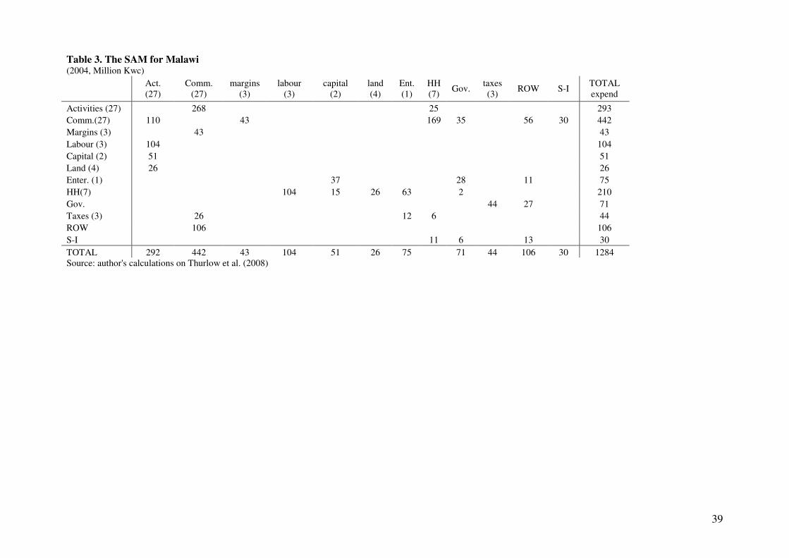
39

Table 3. The SAM for Malawi (2004, Million Kwc)

Act.

(27)

Comm.

(27)

margins

(3)

labour

(3)

capital

(2)

land

(4)

Ent.

(1)

HH

(7) Gov.

taxes

(3) ROW S-I

TOTAL

expend

Activities (27) 268 25 293

Comm.(27) 110 43 169 35 56 30 442

Margins (3) 43 43

Labour (3) 104 104

Capital (2) 51 51

Land (4) 26 26

Enter. (1) 37 28 11 75

HH(7) 104 15 26 63 2 210

Gov. 44 27 71

Taxes (3) 26 12 6 44

ROW 106 106

S-I 11 6 13 30

TOTAL 292 442 43 104 51 26 75 71 44 106 30 1284

Source: author's calculations on Thurlow et al. (2008)

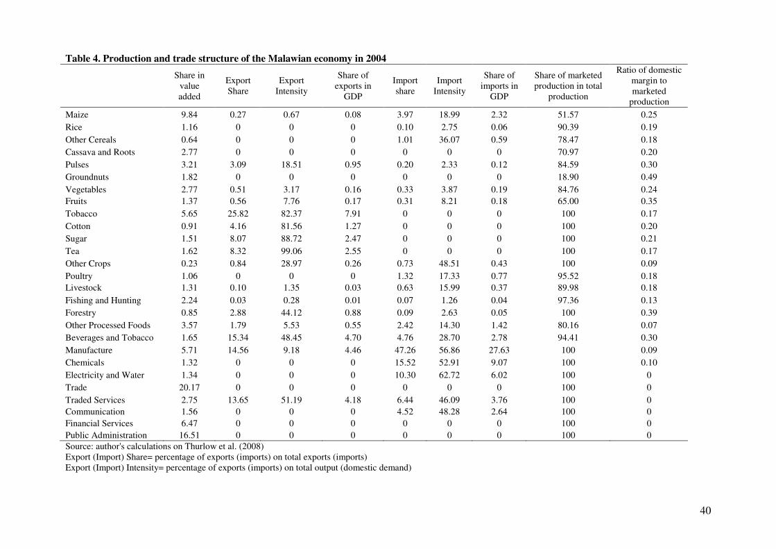
40

Table 4. Production and trade structure of the Malawian economy in 2004

Share in

value

added

Export

Share

Export

Intensity

Share of

exports in

GDP

Import

share

Import

Intensity

Share of

imports in

GDP

Share of marketed

production in total

production

Ratio of domestic

margin to

marketed

production

Maize 9.84 0.27 0.67 0.08 3.97 18.99 2.32 51.57 0.25

Rice 1.16 0 0 0 0.10 2.75 0.06 90.39 0.19

Other Cereals 0.64 0 0 0 1.01 36.07 0.59 78.47 0.18

Cassava and Roots 2.77 0 0 0 0 0 0 70.97 0.20

Pulses 3.21 3.09 18.51 0.95 0.20 2.33 0.12 84.59 0.30

Groundnuts 1.82 0 0 0 0 0 0 18.90 0.49

Vegetables 2.77 0.51 3.17 0.16 0.33 3.87 0.19 84.76 0.24

Fruits 1.37 0.56 7.76 0.17 0.31 8.21 0.18 65.00 0.35

Tobacco 5.65 25.82 82.37 7.91 0 0 0 100 0.17

Cotton 0.91 4.16 81.56 1.27 0 0 0 100 0.20

Sugar 1.51 8.07 88.72 2.47 0 0 0 100 0.21

Tea 1.62 8.32 99.06 2.55 0 0 0 100 0.17

Other Crops 0.23 0.84 28.97 0.26 0.73 48.51 0.43 100 0.09

Poultry 1.06 0 0 0 1.32 17.33 0.77 95.52 0.18

Livestock 1.31 0.10 1.35 0.03 0.63 15.99 0.37 89.98 0.18

Fishing and Hunting 2.24 0.03 0.28 0.01 0.07 1.26 0.04 97.36 0.13

Forestry 0.85 2.88 44.12 0.88 0.09 2.63 0.05 100 0.39

Other Processed Foods 3.57 1.79 5.53 0.55 2.42 14.30 1.42 80.16 0.07

Beverages and Tobacco 1.65 15.34 48.45 4.70 4.76 28.70 2.78 94.41 0.30

Manufacture 5.71 14.56 9.18 4.46 47.26 56.86 27.63 100 0.09

Chemicals 1.32 0 0 0 15.52 52.91 9.07 100 0.10

Electricity and Water 1.34 0 0 0 10.30 62.72 6.02 100 0

Trade 20.17 0 0 0 0 0 0 100 0

Traded Services 2.75 13.65 51.19 4.18 6.44 46.09 3.76 100 0

Communication 1.56 0 0 0 4.52 48.28 2.64 100 0

Financial Services 6.47 0 0 0 0 0 0 100 0

Public Administration 16.51 0 0 0 0 0 0 100 0

Source: author's calculations on Thurlow et al. (2008)

Export (Import) Share= percentage of exports (imports) on total exports (imports)

Export (Import) Intensity= percentage of exports (imports) on total output (domestic demand)

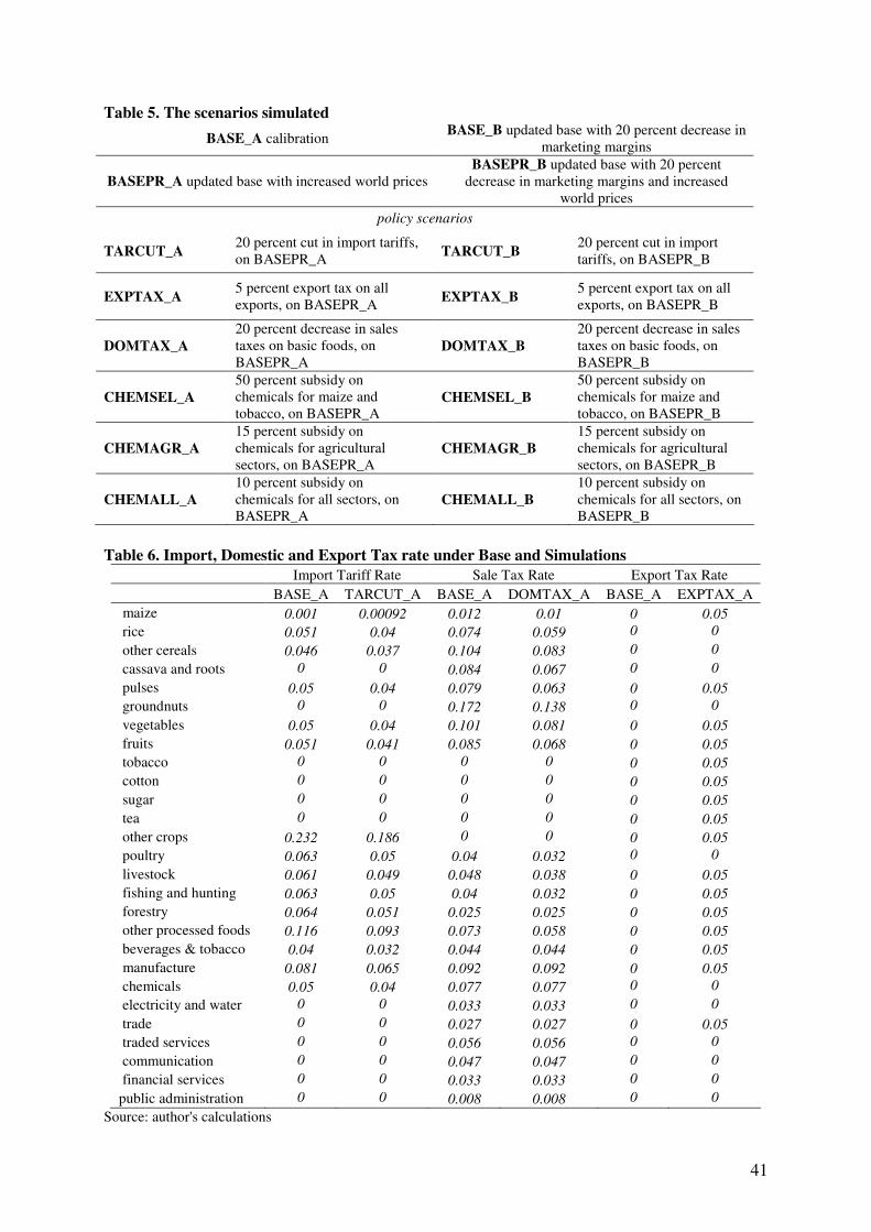
41

Table 5. The scenarios simulated

BASE_A calibration BASE_B updated base with 20 percent decrease in

marketing margins

BASEPR_A updated base with increased world prices

BASEPR_B updated base with 20 percent

decrease in marketing margins and increased

world prices

policy scenarios

TARCUT_A 20 percent cut in import tariffs,

on BASEPR_A TARCUT_B

20 percent cut in import

tariffs, on BASEPR_B

EXPTAX_A 5 percent export tax on all

exports, on BASEPR_A EXPTAX_B

5 percent export tax on all

exports, on BASEPR_B

DOMTAX_A

20 percent decrease in sales

taxes on basic foods, on

BASEPR_A

DOMTAX_B

20 percent decrease in sales

taxes on basic foods, on

BASEPR_B

CHEMSEL_A

50 percent subsidy on

chemicals for maize and

tobacco, on BASEPR_A CHEMSEL_B

50 percent subsidy on

chemicals for maize and

tobacco, on BASEPR_B

CHEMAGR_A

15 percent subsidy on

chemicals for agricultural

sectors, on BASEPR_A

CHEMAGR_B

15 percent subsidy on

chemicals for agricultural

sectors, on BASEPR_B

CHEMALL_A

10 percent subsidy on

chemicals for all sectors, on

BASEPR_A CHEMALL_B

10 percent subsidy on

chemicals for all sectors, on

BASEPR_B

Table 6. Import, Domestic and Export Tax rate under Base and Simulations

Import Tariff Rate Sale Tax Rate Export Tax Rate

BASE_A TARCUT_A BASE_A DOMTAX_A BASE_A EXPTAX_A

maize 0.001 0.00092 0.012 0.01 0 0.05

rice 0.051 0.04 0.074 0.059 0 0

other cereals 0.046 0.037 0.104 0.083 0 0

cassava and roots 0 0 0.084 0.067 0 0

pulses 0.05 0.04 0.079 0.063 0 0.05

groundnuts 0 0 0.172 0.138 0 0

vegetables 0.05 0.04 0.101 0.081 0 0.05

fruits 0.051 0.041 0.085 0.068 0 0.05

tobacco 0 0 0 0 0 0.05

cotton 0 0 0 0 0 0.05

sugar 0 0 0 0 0 0.05

tea 0 0 0 0 0 0.05

other crops 0.232 0.186 0 0 0 0.05

poultry 0.063 0.05 0.04 0.032 0 0

livestock 0.061 0.049 0.048 0.038 0 0.05

fishing and hunting 0.063 0.05 0.04 0.032 0 0.05

forestry 0.064 0.051 0.025 0.025 0 0.05

other processed foods 0.116 0.093 0.073 0.058 0 0.05

beverages & tobacco 0.04 0.032 0.044 0.044 0 0.05

manufacture 0.081 0.065 0.092 0.092 0 0.05

chemicals 0.05 0.04 0.077 0.077 0 0

electricity and water 0 0 0.033 0.033 0 0

trade 0 0 0.027 0.027 0 0.05

traded services 0 0 0.056 0.056 0 0

communication 0 0 0.047 0.047 0 0

financial services 0 0 0.033 0.033 0 0

public administration 0 0 0.008 0.008 0 0

Source: author's calculations

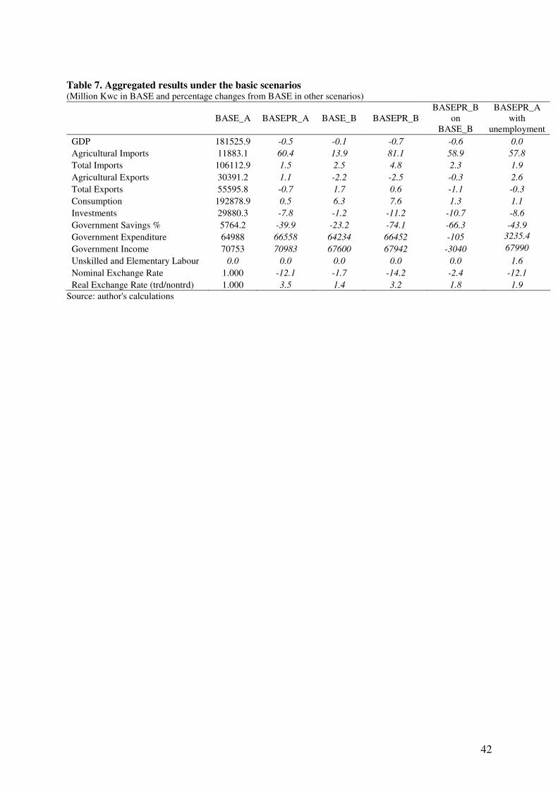
42

Table 7. Aggregated results under the basic scenarios (Million Kwc in BASE and percentage changes from BASE in other scenarios)

BASE_A BASEPR_A BASE_B BASEPR_B

BASEPR_B

on

BASE_B

BASEPR_A

with

unemployment

GDP 181525.9 -0.5 -0.1 -0.7 -0.6 0.0

Agricultural Imports 11883.1 60.4 13.9 81.1 58.9 57.8

Total Imports 106112.9 1.5 2.5 4.8 2.3 1.9

Agricultural Exports 30391.2 1.1 -2.2 -2.5 -0.3 2.6

Total Exports 55595.8 -0.7 1.7 0.6 -1.1 -0.3

Consumption 192878.9 0.5 6.3 7.6 1.3 1.1

Investments 29880.3 -7.8 -1.2 -11.2 -10.7 -8.6

Government Savings % 5764.2 -39.9 -23.2 -74.1 -66.3 -43.9

Government Expenditure 64988 66558 64234 66452 -105 3235.4

Government Income 70753 70983 67600 67942 -3040 67990

Unskilled and Elementary Labour 0.0 0.0 0.0 0.0 0.0 1.6

Nominal Exchange Rate 1.000 -12.1 -1.7 -14.2 -2.4 -12.1

Real Exchange Rate (trd/nontrd) 1.000 3.5 1.4 3.2 1.8 1.9

Source: author's calculations

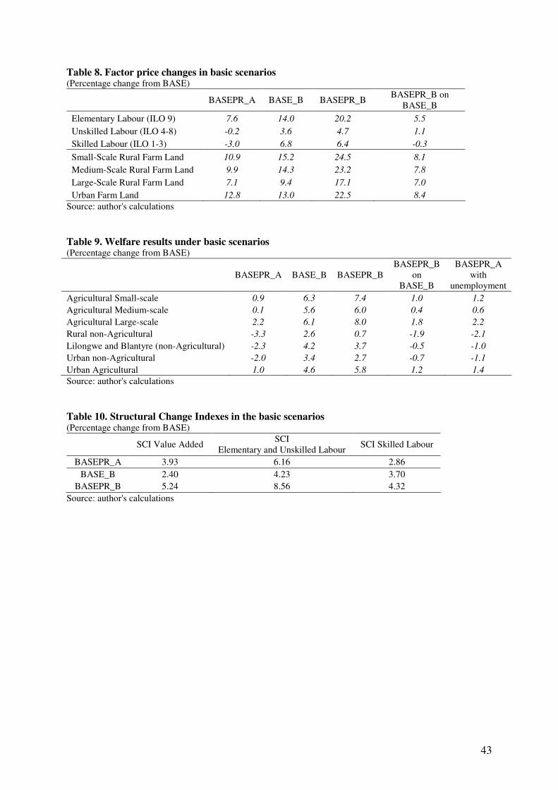
43

Table 8. Factor price changes in basic scenarios (Percentage change from BASE)

BASEPR_A BASE_B BASEPR_B

BASEPR_B on

BASE_B

Elementary Labour (ILO 9) 7.6 14.0 20.2 5.5

Unskilled Labour (ILO 4-8) -0.2 3.6 4.7 1.1

Skilled Labour (ILO 1-3) -3.0 6.8 6.4 -0.3

Small-Scale Rural Farm Land 10.9 15.2 24.5 8.1

Medium-Scale Rural Farm Land 9.9 14.3 23.2 7.8

Large-Scale Rural Farm Land 7.1 9.4 17.1 7.0

Urban Farm Land 12.8 13.0 22.5 8.4

Source: author's calculations

Table 9. Welfare results under basic scenarios (Percentage change from BASE)

BASEPR_A BASE_B BASEPR_B

BASEPR_B

on

BASE_B

BASEPR_A

with

unemployment

Agricultural Small-scale 0.9 6.3 7.4 1.0 1.2

Agricultural Medium-scale 0.1 5.6 6.0 0.4 0.6

Agricultural Large-scale 2.2 6.1 8.0 1.8 2.2

Rural non-Agricultural -3.3 2.6 0.7 -1.9 -2.1

Lilongwe and Blantyre (non-Agricultural) -2.3 4.2 3.7 -0.5 -1.0

Urban non-Agricultural -2.0 3.4 2.7 -0.7 -1.1

Urban Agricultural 1.0 4.6 5.8 1.2 1.4

Source: author's calculations

Table 10. Structural Change Indexes in the basic scenarios (Percentage change from BASE)

SCI Value Added SCI

Elementary and Unskilled Labour SCI Skilled Labour

BASEPR_A 3.93 6.16 2.86

BASE_B 2.40 4.23 3.70

BASEPR_B 5.24 8.56 4.32

Source: author's calculations

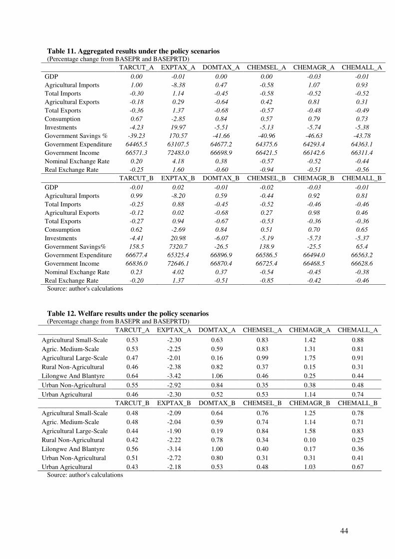
44

Table 11. Aggregated results under the policy scenarios (Percentage change from BASEPR and BASEPRTD)

TARCUT_A EXPTAX_A DOMTAX_A CHEMSEL_A CHEMAGR_A CHEMALL_A

GDP 0.00 -0.01 0.00 0.00 -0.03 -0.01

Agricultural Imports 1.00 -8.38 0.47 -0.58 1.07 0.93

Total Imports -0.30 1.14 -0.45 -0.58 -0.52 -0.52

Agricultural Exports -0.18 0.29 -0.64 0.42 0.81 0.31

Total Exports -0.36 1.37 -0.68 -0.57 -0.48 -0.49

Consumption 0.67 -2.85 0.84 0.57 0.79 0.73

Investments -4.23 19.97 -5.51 -5.13 -5.74 -5.38

Government Savings % -39.23 170.57 -41.66 -40.96 -46.63 -43.78

Government Expenditure 64465.5 63107.5 64677.2 64375.6 64293.4 64363.1

Government Income 66571.3 72483.0 66698.9 66421.5 66142.6 66311.4

Nominal Exchange Rate 0.20 4.18 0.38 -0.57 -0.52 -0.44

Real Exchange Rate -0.25 1.60 -0.60 -0.94 -0.51 -0.56

TARCUT_B EXPTAX_B DOMTAX_B CHEMSEL_B CHEMAGR_B CHEMALL_B

GDP -0.01 0.02 -0.01 -0.02 -0.03 -0.01

Agricultural Imports 0.99 -8.20 0.59 -0.44 0.92 0.81

Total Imports -0.25 0.88 -0.45 -0.52 -0.46 -0.46

Agricultural Exports -0.12 0.02 -0.68 0.27 0.98 0.46

Total Exports -0.27 0.94 -0.67 -0.53 -0.36 -0.36

Consumption 0.62 -2.69 0.84 0.51 0.70 0.65

Investments -4.41 20.98 -6.07 -5.19 -5.73 -5.37

Government Savings% 158.5 7320.7 -26.5 138.9 -25.5 65.4

Government Expenditure 66677.4 65325.4 66896.9 66586.5 66494.0 66563.2

Government Income 66836.0 72646.1 66870.4 66725.4 66468.5 66628.6

Nominal Exchange Rate 0.23 4.02 0.37 -0.54 -0.45 -0.38

Real Exchange Rate -0.20 1.37 -0.51 -0.85 -0.42 -0.46

Source: author's calculations

Table 12. Welfare results under the policy scenarios (Percentage change from BASEPR and BASEPRTD)

TARCUT_A EXPTAX_A DOMTAX_A CHEMSEL_A CHEMAGR_A CHEMALL_A

Agricultural Small-Scale 0.53 -2.30 0.63 0.83 1.42 0.88

Agric. Medium-Scale 0.53 -2.25 0.59 0.83 1.31 0.81

Agricultural Large-Scale 0.47 -2.01 0.16 0.99 1.75 0.91

Rural Non-Agricultural 0.46 -2.38 0.82 0.37 0.15 0.31

Lilongwe And Blantyre 0.64 -3.42 1.06 0.46 0.25 0.44

Urban Non-Agricultural 0.55 -2.92 0.84 0.35 0.38 0.48

Urban Agricultural 0.46 -2.30 0.52 0.53 1.14 0.74

TARCUT_B EXPTAX_B DOMTAX_B CHEMSEL_B CHEMAGR_B CHEMALL_B

Agricultural Small-Scale 0.48 -2.09 0.64 0.76 1.25 0.78

Agric. Medium-Scale 0.48 -2.04 0.59 0.74 1.14 0.71

Agricultural Large-Scale 0.44 -1.90 0.19 0.84 1.58 0.83

Rural Non-Agricultural 0.42 -2.22 0.78 0.34 0.10 0.25

Lilongwe And Blantyre 0.56 -3.14 1.00 0.40 0.17 0.36

Urban Non-Agricultural 0.51 -2.72 0.80 0.31 0.31 0.41

Urban Agricultural 0.43 -2.18 0.53 0.48 1.03 0.67

Source: author's calculations

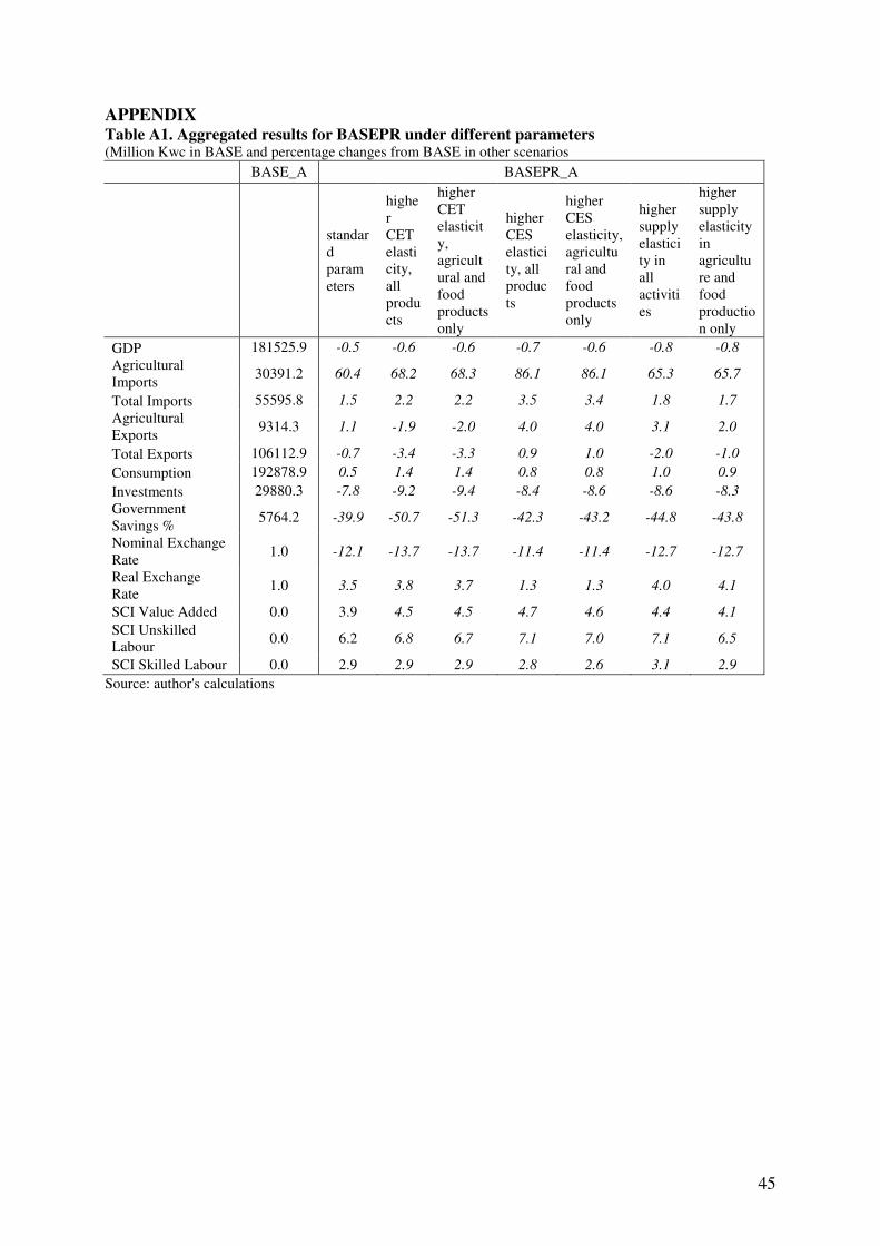
45

APPENDIX Table A1. Aggregated results for BASEPR under different parameters (Million Kwc in BASE and percentage changes from BASE in other scenarios

BASE_A BASEPR_A

standar

d

param

eters

highe

r

CET

elasti

city,

all

produ

cts

higher

CET

elasticit

y,

agricult

ural and

food

products

only

higher

CES

elastici

ty, all

produc

ts

higher

CES

elasticity,

agricultu

ral and

food

products

only

higher

supply

elastici

ty in

all

activiti

es

higher

supply

elasticity

in

agricultu

re and

food

productio

n only

GDP 181525.9 -0.5 -0.6 -0.6 -0.7 -0.6 -0.8 -0.8

Agricultural

Imports 30391.2 60.4 68.2 68.3 86.1 86.1 65.3 65.7

Total Imports 55595.8 1.5 2.2 2.2 3.5 3.4 1.8 1.7

Agricultural

Exports 9314.3 1.1 -1.9 -2.0 4.0 4.0 3.1 2.0

Total Exports 106112.9 -0.7 -3.4 -3.3 0.9 1.0 -2.0 -1.0

Consumption 192878.9 0.5 1.4 1.4 0.8 0.8 1.0 0.9

Investments 29880.3 -7.8 -9.2 -9.4 -8.4 -8.6 -8.6 -8.3

Government

Savings % 5764.2 -39.9 -50.7 -51.3 -42.3 -43.2 -44.8 -43.8

Nominal Exchange

Rate 1.0 -12.1 -13.7 -13.7 -11.4 -11.4 -12.7 -12.7

Real Exchange

Rate 1.0 3.5 3.8 3.7 1.3 1.3 4.0 4.1

SCI Value Added 0.0 3.9 4.5 4.5 4.7 4.6 4.4 4.1

SCI Unskilled

Labour 0.0 6.2 6.8 6.7 7.1 7.0 7.1 6.5

SCI Skilled Labour 0.0 2.9 2.9 2.9 2.8 2.6 3.1 2.9

Source: author's calculations

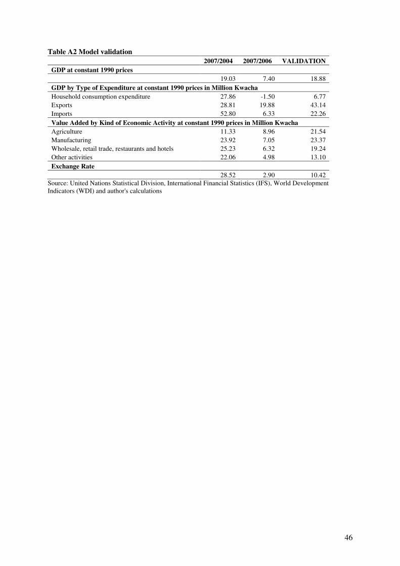
46

Table A2 Model validation

2007/2004 2007/2006 VALIDATION

GDP at constant 1990 prices

19.03 7.40 18.88

GDP by Type of Expenditure at constant 1990 prices in Million Kwacha

Household consumption expenditure 27.86 -1.50 6.77

Exports 28.81 19.88 43.14

Imports 52.80 6.33 22.26

Value Added by Kind of Economic Activity at constant 1990 prices in Million Kwacha

Agriculture 11.33 8.96 21.54

Manufacturing 23.92 7.05 23.37

Wholesale, retail trade, restaurants and hotels 25.23 6.32 19.24

Other activities 22.06 4.98 13.10

Exchange Rate

28.52 2.90 10.42

Source: United Nations Statistical Division, International Financial Statistics (IFS), World Development

Indicators (WDI) and author's calculations