Embed Size (px)
Citation preview
Impact of Unsteady Flow Processes on the Performance of aHigh Speed Axial Flow Compressor
by
Barbara Brenda Botros
B.Eng. Honours, Mechanical Engineering, McGill University, Montreal, Quebec, Canada, 2005
Submitted to the Department of Mechanical Engineeringin partial fulfillment of the requirements for the degree of
Master of Science in Mechanical Engineeringat the
Massachusetts Institute of TechnologyrTewucxry 2oo8]January 2008
2008 Massachusetts Institute of Technology. All Rights Reserved
Author:Department of Mecluanical Engineering
A aJanuary 18, 2008
Certified by:John J. Adamczyk
Distinguished Research Associate, NASA Glenn Research CenterThesis Supervisor
Certified by:.Edward M. Greitzer
H. N. Slater Professor of Aeronautics and AstronauticsThesis Supervisor
Certified by:Choon S. Tan
Senior Research EngineerThesis Supervisor
Read by:John G. Brisson II
Professor of Mechanical Engineering
Accepted by:Lallit Anand
MASSACHLSETTS INST E Chairman, Department Committee on Graduate StudentsOF TECHNOLOGY
JUL 2 9 2008BARKER.
LIBRARIES

MITL bariesDocument Services
Room 14-055177 Massachusetts AvenueCambridge, MA 02139Ph: 617.253.2800Email: [email protected]://Iibraries.mit.edu/docs
DISCLAIMER OF QUALITY
Due to the condition of the original material, there are unavoidableflaws in this reproduction. We have made every effort possible toprovide you with the best copy available. If you are dissatisfied withthis product and find it unusable, please contact Document Services assoon as possible.
Thank you.
The images contained in this document are ofthe best quality available.
Impact of Unsteady Flow Processes on the Performance ofa High Speed Axial Flow Compressor
by
Barbara Brenda Botros
Submitted to the Department of Mechanical Engineering on January 22, 2008 in partialfulfillment of the requirements for the degree of Master of Science
Abstract
This thesis examines the unsteady interactions between blade rows in a high Machnumber, highly-loaded compressor stage. Two straight vane/rotor configurations withdifferent axial spacing between vane and rotor are considered. The numericalsimulations of the two configurations are used to determine the effect of axial blade rowspacing on the level of entropy generation and the flow mechanisms that affect stageperformance. The rotor shock waves that impinge on the upstream blade row result inshed vortices that convect downstream through the rotor. At the reduced axial spacing,vortices with larger circulation and entropy are formed.
Local entropy generation is assessed using a new numerical technique that allowsadequate evaluation of spatial derivatives in high gradient regions, such as shock waves.It is found that the main difference in entropy generation between the two configurationsstudied is associated with the shed vortices. Entropy production and rotor work inputdepend on the vortex trajectory within the rotor, which in turn depends on the ratio oftime scales: the time for vortex convection between blade rows, and the rotor period (i.e.the time for the rotor to move one rotor pitch), for a fixed geometry and inlet Machnumber.
Thesis Supervisor: John J. AdamczykTitle: Distinguished Research Associate, NASA Glenn Research Center
Thesis Supervisor: Edward M. GreitzerTitle: H.N. Slater Professor of Aeronautics and Astronautics
Thesis Supervisor: Choon S. TanTitle: Senior Research Engineer
2
Acknowledgements
I am grateful to all the people who made this work possible. My advisors, Prof.Edward M. Greitzer and Dr. Choon S. Tan, have given me the opportunity to explore aresearch problem without reserve, to be able to make mistakes and learn from them.They have taught me a great deal about the research and writing process that has madethis experience invaluable. Like vorticity, my gratitude to them is endless. To Dr. JohnAdamczyk, a great mentor and friend, my sincerest and warmest thanks for all he hastaught me. With every ten hour tutorial and every cup of tea, he encouraged me to bebetter and work harder.
This thesis would not have been possible without the help of Sean Nolan, who ranthe numerical simulations. I appreciate his guidance and patience throughout this work.I would also like to acknowledge the constructive input from Dr. Steven Gorrell from AirForce Research Laboratory. My gratitude goes to Dr. J.P. Chen, from Ohio StateUniversity, for his assistance using MSU Turbo. I also benefited from discussions withProf. Nick Cumpsty from Imperial College, England about my work.
Many thanks to the students in the Gas Turbine Lab who made this experiencethat much more enjoyable. Alfonso Villanueva, mainly for his visualization codes, butalso for his countless distractions. My right hand, Francois Lefloch, for being the besttutor, director, sounding board, tour guide, and co-member of the Terrible Two I've everhad. Darius Mobed, comedic genius and most potential castaway. Honorable mentionsgo to Mikhael Krotov (best office mate), David Tarr, Angelique Plas, Parthiv Shah, RyanTam, and Isabelle Delefortrie for the good times.
I could not have done this work without the support and encouragement fromfamily and friends. I would like to credit my parents for giving me the perfect name -my initials played nicely into this thesis. I would especially like to thank my dad, Dr.Kamal K. Botros, for being an endless source of guidance and wisdom, for hisencouragement, and for being the ultimate B.F.I.T.
This work was supported by AFOSR grant #FA9550-05-1-0050, under programmanagers Lt. Col. Rhett Jeffries and Dr. Thomas J. Beutner. Additional backing wasprovided by NSERC Canada Postgraduate Scholarships. This support is greatlyappreciated. Numerical simulations were conducted using MSU Turbo.
Disclaimer
The research reported in this document/presentation was performed in connection with the U.S.Air Force Office of Scientific Research, USAF under grant number FA9550-05-1-0050. The views andconclusions contained in this document/presentation are those of the authors and should not be interpretedas presenting the official policies or position, either expressed or implied, of the U.S. Air Force or the U.S.government unless so designated by other authorized documents. Citation of manufacturers' or tradenames does not constitute an official endorsement or approval of the use thereof. The U.S. Government isauthorized to reproduce and distribute reprints notwithstanding any copyright notation hereon.
3
Contents
Abstract 2
Acknowledgements 3
Contents 4
List of Figures 6
List of Tables 8
Nomenclature 9
1 Introduction 11
1.1 Previous Work....................................................... 11
1.2 Present Work.........................................................18
1.3 Technical Objectives................................................19
1.4 Thesis Scope and Content...........................................20
1.5 Research Contributions................................................20
2 Numerical Simulations 21
2.1 N um erical C ode......................................................... 21
2.1.1 Time Discretization and Time-averaging....................23
2.2 Three-dimensional Calculations....................................25
2.2.1 G eom etry ......................................................... 25
2.2.2 Performance Metrics........................................26
4
2.3 Two-dimensional Calculations..................................... 28
2.3.1 G eom etry ......................................................... 28
2.3.2 Performance M etrics........................................ 29
3 Quantification of Entropy Sources 31
3.1 Sources of Entropy Generation.................................... 32
3.2 Numerical Approach to Compute Dissipation...................35
3.3 Procedure to Calculate Shock Entropy Rise...................... 39
4 Vortex Trajectory within the Rotor 45
4.1 Parameters that Impact Vortex Trajectory with the Rotor.......45
4.2 Vortex Trajectories in the Two-dimensional Computations......48
4.3 Vortex Strength and Size in Gap Region.........................50
4.4 Rotor Response to a Change in Vortex Trajectory..............56
4.5 Chapter 4 Sum m ary.................................................... 60
5 Summary and Conclusions 62
6 Suggested Future Work 64
References 66
Appendix A: Non-Uniformity Metric 68
Appendix B: Mixing of Boundary Layers to a Uniform Flow State 74
5
List of Figures
1.1 Effect of axial blade row spacing on performance of a 4-stage compressor [1]......12
1.2 Comparison of wave configurations between the closest and farthest blade row
spacing used in the SM I rig.............................................................. 13
1.3 Rotor shock impinging on the upstream vane row causing a net loading on the blade,
and the form ation of shed vortices.......................................................15
1.4 Isentropic efficiency as a function of axial spacing for transonic operating
conditions [11].......................................................................... . ... 17
2.1 Vane/rotor-only performance from experiment, 100% speed. [211 ................ 27
3.1 Entropy flux as a function of axial location for far and close spacing.............32
3.2 Entropy contours at mid-span for far and close spacing...............................34
3.3 Divergence of velocity contours at mid-span for far and close spacing...............35
3.4 Control volume around rotor shock wave..............................................36
3.5 Comparison of entropy rise calculated from the computational and physical
dissipation in axial gap for far spacing.................................................. 39
3.6 Isolating rotor shock waves. Contour plots of divergence of velocity and
computational dissipation at the mid-span for the far spacing......................... 40
3.7 Profile of divergence of velocity in shock region........................................41
4.1 Different vortex trajectories within the rotor passage due to different axial blade
row spacing................................................................................. 45
4.2 Entropy contours for far2D and close2D------------------................................49
4.3 Time-averaged entropy contours within the rotor passage for far2D and close2D. ... 50
6

4.4 V ortex equivalent radius.................................................................. 52
4.5 Non-uniformity metric as a function of axial position................................55
4.6 Differences in boundary layers between far2D and close2D...........................58
B. 1 Mixing of a swirling flow to a uniform flow state....................................74
7
List of Tables
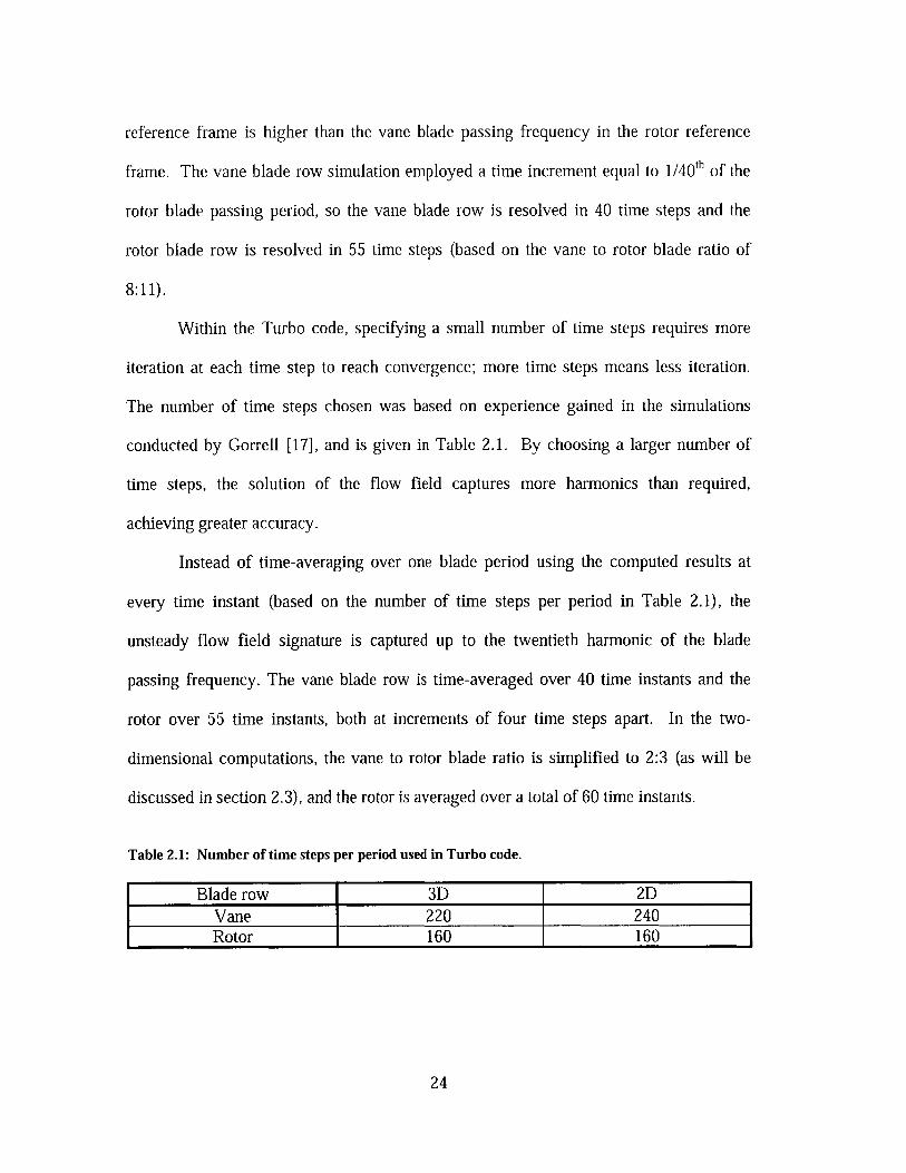
2.1 Number of time steps per period used in Turbo code................................24
2.2 Axial blade row spacing for close and far configurations, normalized by the axial
rotor chord length c ....................................................................... 25
2.3 SMI Aerodynamic Design Parameters [6]..............................................26
2.4 Number of grid points in axial, radial and pitch-wise directions for the three-
dim ensional calculations.....................................................................26
2.5 Mass flow rate, total temperature rise, total pressure ratio, and adiabatic efficiency
from three-dimensional calculations for far and close spacing configurations........ 28
2.6 Number of grid points in axial, radial and pitch-wise directions for the two-
dim ensional calculations.....................................................................29
2.7 Mass flow rate, total temperature rise, and total pressure from two-dimensional
calculations for far2D and close2D configurations.....................................30
2.8 Efficiency for far2D and close2D spacing configurations at the rotor exit and at
dow nstream infinity....................................................................... 30
3.1 Difference in entropy generation within the rotor for the far and close spacings
separated into the differences inside and outside the masked (shock) region........ 43
3.2 Results from Table 3.1, excluding the end wall region.............................. 43
4.1 Circulation for the clockwise vortex at the rotor trailing edge......................51
4.2 Circulation-weighted radii for the clockwise vortex at the rotor trailing edge.......52
4.3 Time-averaged entropy generation in specified control volumes within rotor.......57
4.4 Entropy rise from the rotor trailing edge to far downstream........................ 60
8

Nomenclature
Symbols
p density
p pressure
ft mass flow rate
adiabatic efficiency
CO vorticity
F circulation
L axial gap spacing
C, axial rotor chord length
trailing edge blockage
0 shock angle
Mrei relative Mach number
S entropy
T temperature
p, stagnation pressure
T stagnation temperature
TR stagnation temperature ratio
A area
t time
u velocity
9
mean axial velocity
r stress tensor
k thermal conductivity
A axial direction
y tangential or pitch-wise direction
Q rotor rotational speed
R ideal gas constant
r time period
nblades number of rotor blades
r radius
TC' vorticity-weighted radius
3* displacement thickness
O momentum thickness
0* energy thickness
Subscripts
ref reference conditions
2D two-dimensional geometry
E free stream condition
10
U
Chapter 1
Introduction
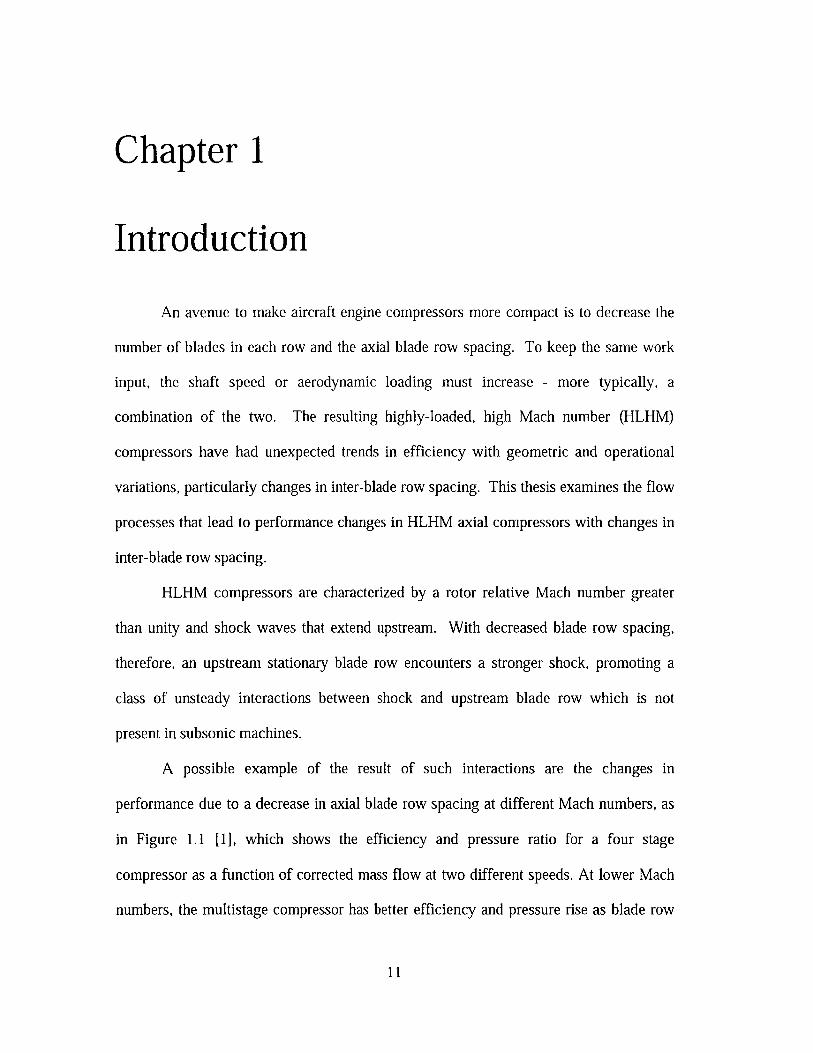
An avenue to make aircraft engine compressors more compact is to decrease the
number of blades in each row and the axial blade row spacing. To keep the same work
input, the shaft speed or aerodynamic loading must increase - more typically, a
combination of the two. The resulting highly-loaded, high Mach number (HLHM)
compressors have had unexpected trends in efficiency with geometric and operational
variations, particularly changes in inter-blade row spacing. This thesis examines the flow
processes that lead to performance changes in HLHM axial compressors with changes in
inter-blade row spacing.
HLHM compressors are characterized by a rotor relative Mach number greater
than unity and shock waves that extend upstream. With decreased blade row spacing,
therefore, an upstream stationary blade row encounters a stronger shock, promoting a
class of unsteady interactions between shock and upstream blade row which is not
present in subsonic machines.
A possible example of the result of such interactions are the changes in
performance due to a decrease in axial blade row spacing at different Mach numbers, as
in Figure 1.1 [1], which shows the efficiency and pressure ratio for a four stage
compressor as a function of corrected mass flow at two different speeds. At lower Mach
numbers, the multistage compressor has better efficiency and pressure rise as blade row
11
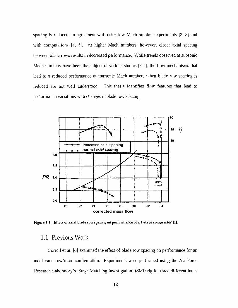
spacing is reduced, in agreement with other low Mach number experiments [2, 3] and
with computations [4, 5]. At higher Mach numbers, however, closer axial spacing
between blade rows results in decreased performance. While trends observed at subsonic
Mach numbers have been the subject of various studies [2-5], the flow mechanisms that
lead to a reduced performance at transonic Mach numbers when blade row spacing is
reduced are not well understood. This thesis identifies flow features that lead to
performance variations with changes in blade row spacing.
PR
4.0
3.5
3.0
2.5
2.0
20
increased axial spacingnormal axial spacing
100%speed
22 24 26 28 30
corrected mass flow
90
8577
80
32 34
Figure 1.1: Effect of axial blade row spacing on performance of a 4-stage compressor [1].
1.1 Previous Work
Gorrell et al. [6] examined the effect of blade row spacing on performance for an
axial vane row/rotor configuration. Experiments were performed using the Air Force
Research Laboratory's 'Stage Matching Investigation' (SMI) rig for three different inter-
12
blade row axial spacings, having a mean (hub-to-tip) value of 13%, 26%, and 55% of the
vane chord [6]. Choking mass flow rate, pressure ratio and efficiency all decreased as
axial spacing was reduced.
Unsteady CFD simulations (using MSU Turbo [7]), conducted for the closest and
farthest spacings of the SMI rig, enabled identification of a loss generating mechanism
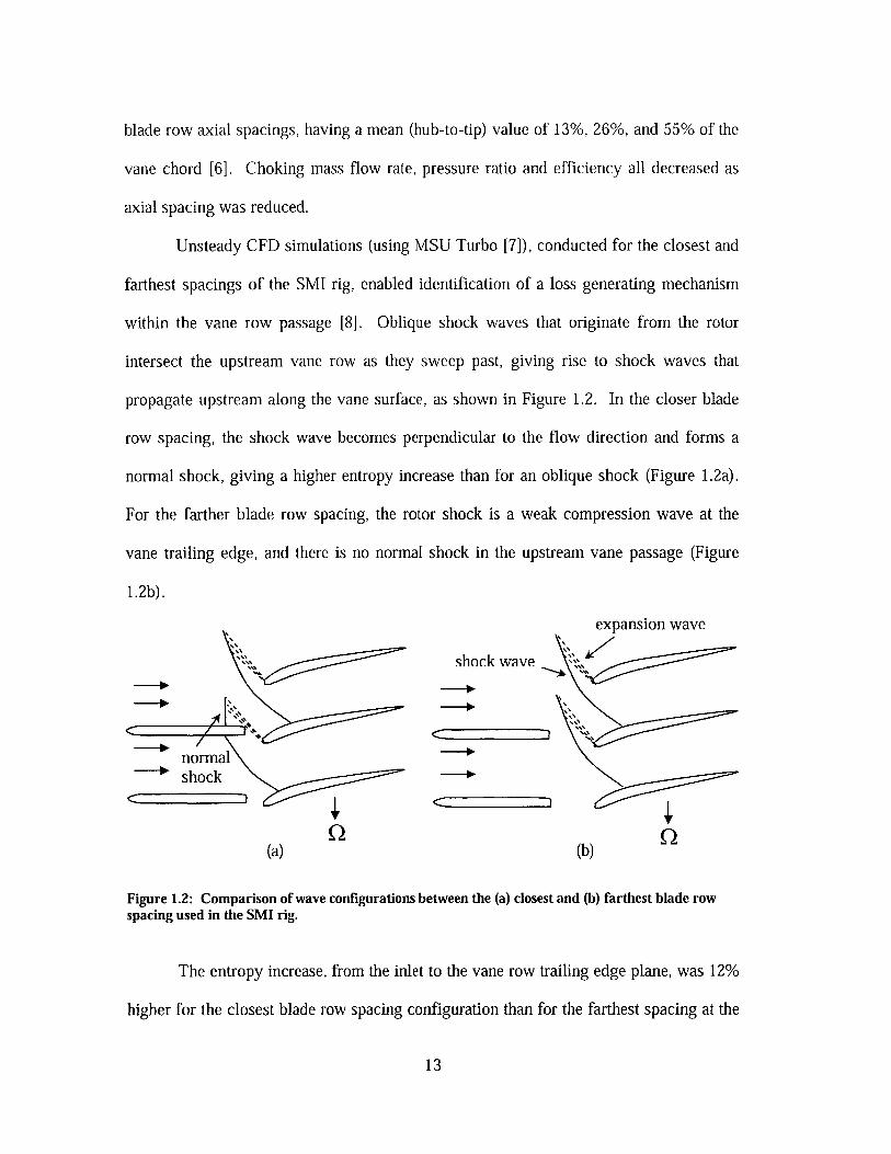
within the vane row passage [8]. Oblique shock waves that originate from the rotor
intersect the upstream vane row as they sweep past, giving rise to shock waves that
propagate upstream along the vane surface, as shown in Figure 1.2. In the closer blade
row spacing, the shock wave becomes perpendicular to the flow direction and forms a
normal shock, giving a higher entropy increase than for an oblique shock (Figure 1.2a).
For the farther blade row spacing, the rotor shock is a weak compression wave at the
vane trailing edge, and there is no normal shock in the upstream vane passage (Figure
1.2b).
normal(shock
(a)
expansion wave
shock wave
(b)
Figure 1.2: Comparison of wave configurations between the (a) closest and (b) farthest blade rowspacing used in the SMI rig.
The entropy increase, from the inlet to the vane row trailing edge plane, was 12%
higher for the closest blade row spacing configuration than for the farthest spacing at the
13
same mass flow rate. Gorrell et al. attributed the additional entropy increase by the vane
trailing edge to the normal shock in the reduced spacing, but a direct link between the
two was not made. Furthermore, the entropy rise from the normal shock alone was not
compared to the total shock losses or to the overall losses for the stage to determine if the
normal shock was the main source of the difference in entropy generation for the
different blade row spacings. The entropy generation from shock waves is assessed in
the present work to determine their impact on performance as a function of blade row
spacing.
In a later work by Gorrell et al. [9], CFD simulations with a more refined grid, as
well as Digital Particle Image Velocimetry (DPIV) measurements, were used to examine
the discrete vortices shed at the vane trailing edge that exist because of the interaction
between the rotor shock and upstream stationary blade row. Within one rotor passing
time, two discrete counter-rotating vortices were found to be shed at the vane trailing
edge. The formation of these vortices can be explained as follows. When the rotor shock
intersects the vane trailing edge, a pressure gradient is established along the surface of the
blade, resulting in a flux of vorticity from the wall into the fluid, and a net circulation
established around the blade. The vorticity generated on the vane is shed from the
trailing edge to form a vortex. As the rotor shock moves past the vane trailing edge, the
pressure gradient along the vane decreases, as does the net circulation, and a discrete
vortex with opposite circulation to the previous one is shed. A vortex street which is
"locked" to the rotor passing is thus formed downstream of the vane trailing edge.
From the above arguments, as the blade row spacing is reduced and there is a
stronger shock impinging on the upstream blade row, there will be a larger pressure
14
gradient and a larger vane circulation. The length scale associated with the vortices is
related to the blade thickness, and thus, a larger vane circulation results in greater
vorticity within the shed vortices. The shed vortices not only contain more vorticity, but
are also observed to have greater entropy as blade row spacing is reduced.
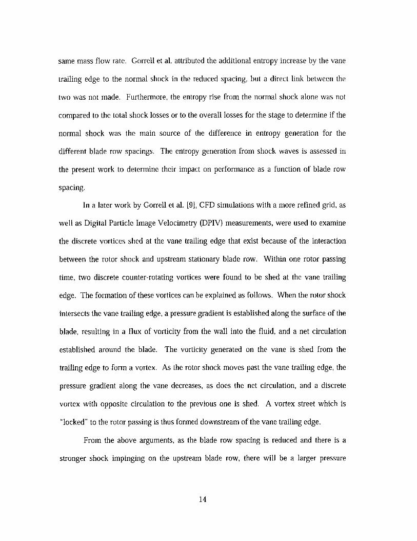
Gorrell et al. [91 developed an analytical relation for the shed vorticity as a
function of vane geometry and rotor shock strength which correlated well with their
computational results. The vorticity within the shed vortices is given as:
;= C X~X5C}(1.1)CO tan#0) p ) m
In equation (1.1), # is the shock angle (see Figure 1.3), Ap/p is the pressure rise across
the shock, -p is the average of the pressures ahead and behind the incoming shock, and
A is the trailing edge blockage, i.e the ratio of trailing edge thickness to pitch. A model
by Morfey and Fischer [101 was used to calculate the shock strength, Ap/ P , as a
function of rotor Mach number, axial flow Mach number, and ratio of the axial distance
ahead of the rotor to rotor pitch.
p+ Ap
yvane rotorAr'' shock
Figure 1.3: Rotor shock impinging on the upstream vane row causing a net loading on the blade, andthe formation of shed vortices.
While the vorticity in the shed vortices was estimated, the entropy generation
associated with the creation of the vortices and the additional losses as they are convected
15
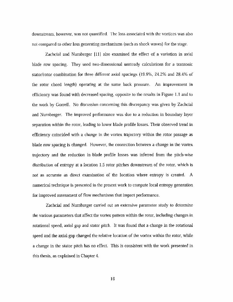
downstream, however, was not quantified. The loss associated with the vortices was also
not compared to other loss generating mechanisms (such as shock waves) for the stage.
Zachcial and Nurnberger [11] also examined the effect of a variation in axial
blade row spacing. They used two-dimensional unsteady calculations for a transonic
stator/rotor combination for three different axial spacings (19.9%, 24.2% and 28.4% of
the rotor chord length) operating at the same back pressure. An improvement in
efficiency was found with decreased spacing, opposite to the results in Figure 1.1 and to
the work by Gorrell. No discussion concerning this discrepancy was given by Zachcial
and Nurnberger. The improved performance was due to a reduction in boundary layer
separation within the rotor, leading to lower blade profile losses. Their observed trend in
efficiency coincided with a change in the vortex trajectory within the rotor passage as
blade row spacing is changed. However, the connection between a change in the vortex
trajectory and the reduction in blade profile losses was inferred from the pitch-wise
distribution of entropy at a location 1.5 rotor pitches downstream of the rotor, which is
not as accurate as direct examination of the location where entropy is created. A
numerical technique is presented in the present work to compute local entropy generation
for improved assessment of flow mechanisms that impact performance.
Zachcial and Nurnburger carried out an extensive parameter study to determine
the various parameters that affect the vortex pattern within the rotor, including changes in
rotational speed, axial gap and stator pitch. It was found that a change in the rotational
speed and the axial gap changed the relative location of the vortex within the rotor, while
a change in the stator pitch has no effect. This is consistent with the work presented in
this thesis, as explained in Chapter 4.
16
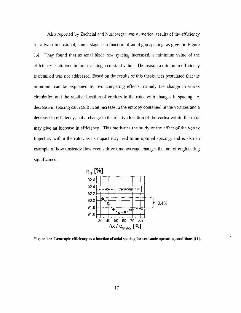
Also reported by Zachcial and Nurnberger was numerical results of the efficiency
for a two-dimensional, single stage as a function of axial gap spacing, as given in Figure
1.4. They found that as axial blade row spacing increased, a minimum value of the
efficiency is attained before reaching a constant value. The reason a minimum efficiency
is obtained was not addressed. Based on the results of this thesis, it is postulated that the
minimum can be explained by two competing effects, namely the change in vortex
circulation and the relative location of vortices in the rotor with changes in spacing. A
decrease in spacing can result in an increase in the entropy contained in the vortices and a
decrease in efficiency, but a change in the relative location of the vortex within the rotor
may give an increase in efficiency. This motivates the study of the effect of the vortex
trajectory within the rotor, as its impact may lead to an optimal spacing, and is also an
example of how unsteady flow events drive time-average changes that are of engineering
significance.
7is [N92.6
92.4r --- 0- - -transonic OPV2.2
92.0:
91. 8
91.6
30 40 50 60 70 80Ax / Cstator [%]
Figure 1.4: Isentropic efficiency as a function of axial spacing for transonic operating conditions [111.
17
-7*10.4%
1.2 Present Work
The focus of the present work is to quantify the dominant entropy generating
mechanism that lead to changes in efficiency, work and pressure rise with axial spacing
between blade rows in a high Mach number, high loading compressor. The relative
importance of proposed entropy generating mechanisms is assessed by computing the
dissipation in the flow field. In this, the primary challenge is to accurately determine the
entropy generation in regions with high spatial gradients, such as shock waves. A
procedure to compute the dissipation from irreversible flow processes, as well as to
isolate the entropy generation across shock waves, is developed. Applying this procedure
to the vane/rotor configuration used in the studies by Gorrell [6, 8-9], it is found that the
majority of the differences in entropy generation that arise from changes in blade row
spacing are associated with the shed vortices. The additional entropy generation created
when blade row spacing is reduced is due to higher circulation (stronger) vortices
diffusing and generating additional loss as they interact with and propagate through the
rotor.
A change in axial blade row spacing has two identifiable impacts on the shed
vortices. First, it changes the circulation of the shed vortices (as identified by Gorrell),
and second, it changes the trajectory of the vortex in the rotor passage. It is shown that
for a given Mach number and geometry, the vortex trajectory within the rotor blade
passage can be described by one compact, non-dimensional quantity. This non-
dimensional quantity is a ratio of two time scales: the rotor period (i.e. the time for the
rotor to move one rotor pitch) and the convective time for the shed vortices to travel the
length of the axial gap. These determine the relative location of the vortices that enter the
18
rotor passage. The vortex trajectory, in turn, can impact the rotor performance as vortices
change the rotor flow field and interact with the rotor boundary layers.
To determine the effect of vortex trajectory on rotor efficiency, two-dimensional
computations were conducted for two different axial blade row spacings. The two blade
row spacings were chosen such that the strength of the rotor shock at the vane row
trailing edge was the same (in order to maintain the same vortex strength). Because of the
trajectory change, however, one configuration had two vortices in the rotor passage core
flow (i.e. outside the boundary layer), while the other had one vortex in the core flow and
one located near the blade surface, mainly within the boundary layer. The largest
difference in entropy generation between the two configurations occurs downstream of
the rotor, due to the mixing of the different flow fields at the rotor trailing edge plane.
1.3 Technical Objectives
In this thesis, mechanisms that impact performance of a transonic rotor due to
changes in upstream blade row spacing are determined. For this, a computational method
is developed to quantify local entropy generation. Isolating the entropy generation
associated with different flow features, including shock waves, was one objective of this
work. A second objective is to determine the impact of vortex trajectory on stage
efficiency, work input and pressure rise.
The research questions to be answered are:
- How do the dominant entropy generation mechanisms vary with axial blade row
spacing?
- What is the performance impact of a change in the trajectory within the rotor of
vortices from the upstream vane row?
19
1.4 Thesis Scope and Content
To answer these research questions, a detailed interrogation of numerical
computations has been carried out. Chapter 2 describes the CFD model, the geometry
and the performance metrics for the computational simulations. Chapter 3 defines a
numerical technique to isolate the regions of entropy generation. In Chapter 4, a non-
dimensional parameter is defined that describes the relative location of vortices in the
rotor, and the performance changes associated with changes in this parameter are
assessed using two-dimensional, unsteady computations. Chapter 5 summarizes the
findings and conclusions, and Chapter 6 gives suggestions for future work.
1.5 Research Contributions
- A framework and computational methodology is developed for quantifying local
entropy generation in transonic compressors, even in regions with high spatial
gradients, such as shock waves.
- The impact of vortex trajectory within the rotor passage on rotor efficiency,
pressure rise and work input is determined. A non-dimensional parameter to
characterize the trajectory of the vortices is defined.
20
Chapter 2
Numerical Simulations
Numerical simulations were conducted to answer the research questions outlined
in the previous chapter. To determine the entropy generating mechanisms responsible for
the change in compressor performance with axial spacing, three-dimensional calculations
were performed using the geometry and code employed by Gorrell [6, 8-9]. The effect of
a change in the vortex trajectory within the rotor was studied via two-dimensional
calculations. The present chapter describes the CFD code, the geometries, and the
performance metrics for the numerical computations.
2.1 Numerical Code
Numerical simulations were conducted using MSU Turbo Version 4.1 [71, an
unsteady, three-dimensional, viscous code that solves the Reynolds Averaged Navier-
Stokes (RANS) equations. The equations are solved in the reference frame of each blade
row. The code employs a finite volume solver, with a K-C turbulence model.
Communication between blade rows in their respective reference frames occurs across a
sliding plane that interpolates information from one blade row to the other.
To reduce computer time and memory required to perform the numerical
experiments, temporal phase lag boundary conditions were used [12-15]. Temporal
phase lag boundary conditions rely on the assumption that the flow field associated with
21
two interacting blade rows has a temporal periodicity related to the blade count of the
blade rows. More specifically, the flow field within the blade passage will repeat itself
every time the relative position of the adjacent blade row is the same. The phase lag
approximation permits the replacement of a full wheel or spatially periodic computation
by a single blade passage within each blade row. The current geometry has 24 stator and
33 rotor blades. If periodic boundary conditions were used, a sector with 8 stator blades
and 11 rotor blades would be required, implying much more computational time and
computer memory than simulations with the temporal phase lag approximation. Using
the phase lag approximation, a full wheel can be constructed at any instant in time using
the computed flow field of the individual passage from previous instants in time. Details
of the full wheel reconstruction are given by Wang and Chen [15].
An assumption associated with the use of phase lag boundary conditions is that
the lowest frequency of any important unsteady phenomenon is the blade-passing
frequency of the adjacent blade row. For example, vortex shedding, rotating stall, or flow
separation that is at a lower frequency than the blade passing frequency would not be
captured. Use of the phase lag boundary condition is an appropriate approximation for
unsteady blade row interactions where the frequency of unsteadiness in one blade row is
dominated by the adjacent blade row passing frequency. The results from phase lag
computations and experiment have been compared in a previous study [9], and the phase
lag approximation captured the flow features that arise from the blade row interactions,
including the vortex shedding from the inlet vanes due to the impingement of the rotor
shock on the vane.
22
Uniform stagnation pressure and temperature are specified at the inlet of the
computational domain. For three-dimensional simulations, at the exit of the
computational domain, the static pressure at the hub is specified, and simple radial
equilibrium is used to specify the radial distribution of static pressure. For the two-
dimensional simulations, the static pressure is specified at the exit. The convergence
criteria was that the time-averaged mass flow rate at the vane row inlet and at the exit of
the domain were within 0.1% of each other, and that the efficiency and mass flow were
periodic with blade passing frequency.
Turbo solves the flow field using primitive variables at cell centers. The Turbo
output data is therefore chosen to be the values at the cell center (instead of using the
conventional Plot3D output, which interpolates to cell nodes). Use of cell-center output
means that information is not lost in the interpolation scheme associated with Plot3D.
Visualization of the output was accomplished with the codes developed by Villanueva
[16].
2.1.1 Time Discretization and Time-averaging
The number of time steps for each blade period was chosen based on the desired
temporal resolution of the blade row interactions. The frequency of unsteadiness within
one blade row is determined by the blade passing frequency of the adjacent blade row,
and resolving twenty harmonics of the blade passing frequency should well capture the
flow features deriving from unsteady blade row interactions, including vortex shedding.
According to Nyquist's theorem, a harmonic must be sampled at least twice per cycle in
order to be resolved, so 40 samples were taken for one blade-passing period. In the
vane/rotor configuration studied here, the rotor blade passing frequency in the vane
23
reference frame is higher than the vane blade passing frequency in the rotor reference
frame. The vane blade row simulation employed a time increment equal to 1/40 of the
rotor blade passing period, so the vane blade row is resolved in 40 time steps and the
rotor blade row is resolved in 55 time steps (based on the vane to rotor blade ratio of
8:11).
Within the Turbo code, specifying a small number of time steps requires more
iteration at each time step to reach convergence; more time steps means less iteration.
The number of time steps chosen was based on experience gained in the simulations
conducted by Gorrell [17], and is given in Table 2.1. By choosing a larger number of
time steps, the solution of the flow field captures more harmonics than required,
achieving greater accuracy.
Instead of time-averaging over one blade period using the computed results at
every time instant (based on the number of time steps per period in Table 2.1), the
unsteady flow field signature is captured up to the twentieth harmonic of the blade
passing frequency. The vane blade row is time-averaged over 40 time instants and the
rotor over 55 time instants, both at increments of four time steps apart. In the two-
dimensional computations, the vane to rotor blade ratio is simplified to 2:3 (as will be
discussed in section 2.3), and the rotor is averaged over a total of 60 time instants.
Table 2.1: Number of time steps per period used in Turbo code.
Blade row 3D 2DVane 220 240Rotor 160 160
24
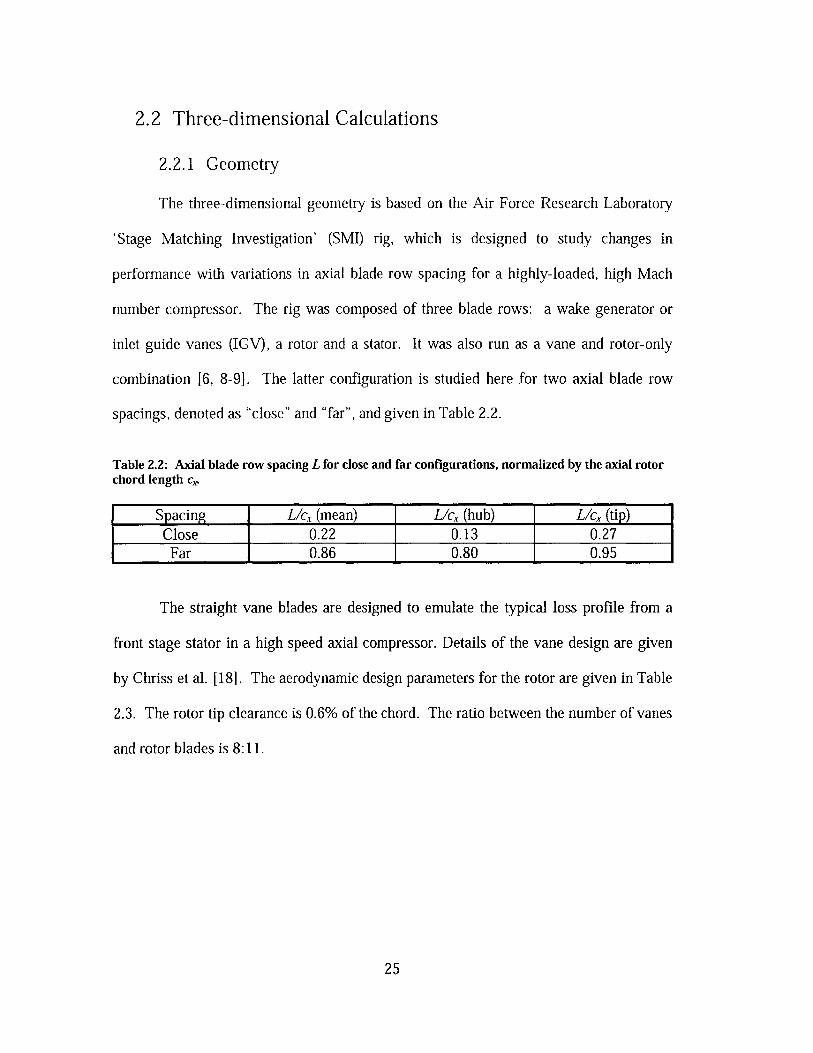
2.2 Three-dimensional Calculations
2.2.1 Geometry
The three-dimensional geometry is based on the Air Force Research Laboratory
'Stage Matching Investigation' (SMI) rig, which is designed to study changes in
performance with variations in axial blade row spacing for a highly-loaded, high Mach
number compressor. The rig was composed of three blade rows: a wake generator or
inlet guide vanes (IGV), a rotor and a stator. It was also run as a vane and rotor-only
combination [6, 8-9]. The latter configuration is studied here for two axial blade row
spacings, denoted as "close" and "far", and given in Table 2.2.
Table 2.2: Axial blade row spacing L for close and far configurations, normalized by the axial rotorchord length c,.
Spacing L/c, (mean) L/c, (hub) L/cX (tip)Close 0.22 0.13 0.27Far 0.86 0.80 0.95
The straight vane blades are designed to emulate the typical loss profile from a
front stage stator in a high speed axial compressor. Details of the vane design are given
by Chriss et al. [18]. The aerodynamic design parameters for the rotor are given in Table
2.3. The rotor tip clearance is 0.6% of the chord. The ratio between the number of vanes
and rotor blades is 8:11.
25
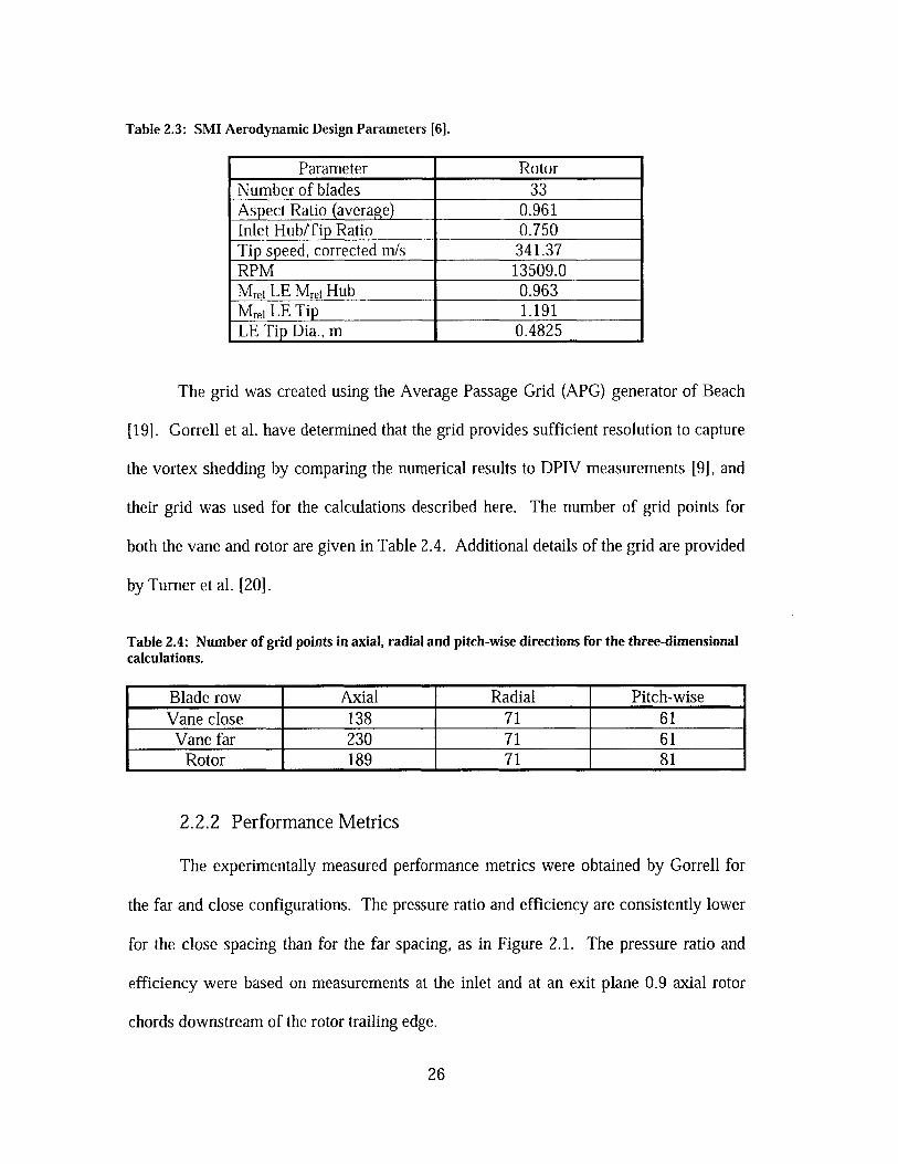
Table 2.3: SMI Aerodynamic Design Parameters [6].
Parameter RotorNumber of blades 33Aspect Ratio (average) 0.961Inlet Hub/Tip Ratio 0.750Tip speed, corrected m/s 341.37RPM 13509.0Mrei LE Mrei Hub 0.963Mrei LE Tip 1.191LE Tip Dia., m 0.4825
The grid was created using the Average Passage Grid (APG) generator of Beach
[19]. Gorrell et al. have determined that the grid provides sufficient resolution to capture
the vortex shedding by comparing the numerical results to DPIV measurements [9], and
their grid was used for the calculations described here. The number of grid points for
both the vane and rotor are given in Table 2.4. Additional details of the grid are provided
by Turner et al. [20].
Table 2.4: Number of grid points in axial, radial and pitch-wise directions for the three-dimensionalcalculations.
Blade row Axial Radial Pitch-wiseVane close 138 71 61Vane far 230 71 61
Rotor 189 71 81
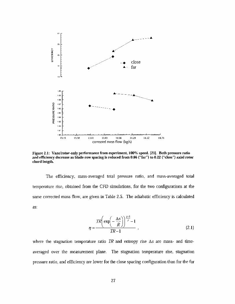
2.2.2 Performance Metrics
The experimentally measured performance metrics were obtained by Gorrell for
the far and close configurations. The pressure ratio and efficiency are consistently lower
for the close spacing than for the far spacing, as in Figure 2.1. The pressure ratio and
efficiency were based on measurements at the inlet and at an exit plane 0.9 axial rotor
chords downstream of the rotor trailing edge.
26
87
86
85
close84 -- A- afar
83
1.90 -
1.89
1.88 -
.187
1.86 -
M 1.85 -
V) 1.84
Ce 1.83
1.82 L
1.81
1.80--II
13.15 13.38 13.61 13.83 14.06 14.29 14.52 14.74
corrected mass flow (kg/s)
Figure 2.1: Vane/rotor-only performance from experiment, 100% speed. [21]. Both pressure ratioand efficiency decrease as blade-row spacing is reduced from 0.86 ("far") to 0.22 ("close") axial rotorchord length.
The efficiency, mass-averaged total pressure ratio, and mass-averaged total
temperature rise, obtained from the CFD simulations, for the two configurations at the
same corrected mass flow, are given in Table 2.5. The adiabatic efficiency is calculated
as:
TRA ex Y-1
77 = Rep-R) (2.1)TR-1
where the stagnation temperature ratio TR and entropy rise As are mass- and time-
averaged over the measurement plane. The stagnation temperature rise, stagnation
pressure ratio, and efficiency are lower for the close spacing configuration than for the far
27
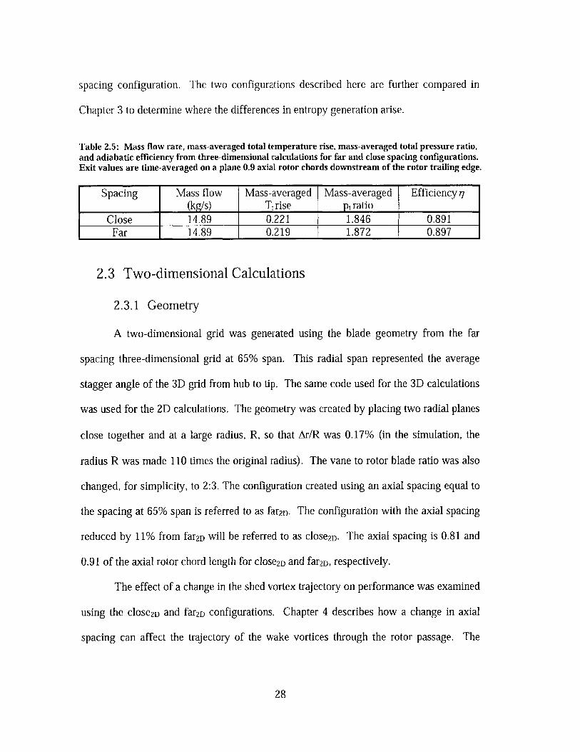
spacing configuration. The two configurations described here are further compared in
Chapter 3 to determine where the differences in entropy generation arise.
Table 2.5: Mass flow rate, mass-averaged total temperature rise, mass-averaged total pressure ratio,and adiabatic efficiency from three-dimensional calculations for far and close spacing configurations.Exit values are time-averaged on a plane 0.9 axial rotor chords downstream of the rotor trailing edge.
Spacing Mass flow Mass-averaged Mass-averaged Efficiency 7(kg/s) Tt rise pt ratio
Close 14.89 0.221 1.846 0.891Far 14.89 0.219 1.872 0.897
2.3 Two-dimensional Calculations
2.3.1 Geometry
A two-dimensional grid was generated using the blade geometry from the far
spacing three-dimensional grid at 65% span. This radial span represented the average
stagger angle of the 3D grid from hub to tip. The same code used for the 3D calculations
was used for the 2D calculations. The geometry was created by placing two radial planes
close together and at a large radius, R, so that Ar/R was 0.17% (in the simulation, the
radius R was made 110 times the original radius). The vane to rotor blade ratio was also
changed, for simplicity, to 2:3. The configuration created using an axial spacing equal to
the spacing at 65% span is referred to as far2D. The configuration with the axial spacing
reduced by 11% from far2D will be referred to as close2D. The axial spacing is 0.81 and
0.91 of the axial rotor chord length for close2D and far2D, respectively.
The effect of a change in the shed vortex trajectory on performance was examined
using the close2D and far2D configurations. Chapter 4 describes how a change in axial
spacing can affect the trajectory of the wake vortices through the rotor passage. The
28
spacing change was chosen such that the rotor shock strength at the vane trailing edge
plane (which set the strength of the shed vortices) differed by less than 2%. The
difference in Mach number at the vane trailing edge plane between the two
configurations was 0.01 (the Mach number is 1.05 in close2D and 1.06 in far2D).
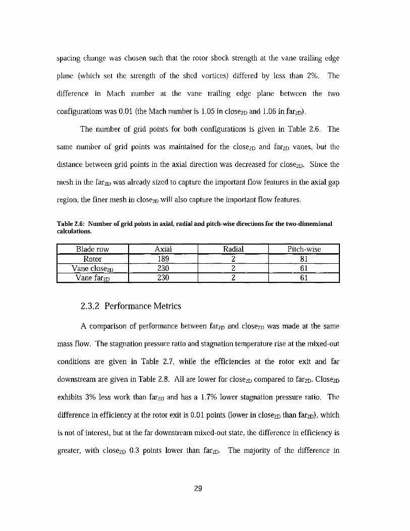
The number of grid points for both configurations is given in Table 2.6. The
same number of grid points was maintained for the close2D and far2D vanes, but the
distance between grid points in the axial direction was decreased for close2D. Since the
mesh in the far2D was already sized to capture the important flow features in the axial gap
region, the finer mesh in close2D will also capture the important flow features.
Table 2.6: Number of grid points in axial, radial and pitch-wise directions for the two-dimensionalcalculations.
Blade row Axial Radial Pitch-wiseRotor 189 2 81
Vane close2D 230 2 61Vane far2D 230 2 61
2.3.2 Performance Metrics
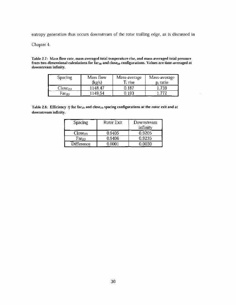
A comparison of performance between far2D and close2D was made at the same
mass flow. The stagnation pressure ratio and stagnation temperature rise at the mixed-out
conditions are given in Table 2.7, while the efficiencies at the rotor exit and far
downstream are given in Table 2.8. All are lower for close2D compared to far2D. Close2D
exhibits 3% less work than far2D and has a 1.7% lower stagnation pressure ratio. The
difference in efficiency at the rotor exit is 0.01 points (lower in close2D than far2D), which
is not of interest, but at the far downstream mixed-out state, the difference in efficiency is
greater, with close2D 0.3 points lower than far2D. The majority of the difference in
29
entropy generation thus occurs downstream of the rotor trailing edge, as is discussed in
Chapter 4.
Table 2.7: Mass flow rate, mass-averaged total temperature rise, and mass-averaged total pressurefrom two-dimensional calculations for far2D and close2D configurations. Values are time-averaged atdownstream infinity.
Spacing Mass flow Mass-average Mass-average(kg/s) Tt rise pt ratio
Close2D 1148.47 0.187 1.739Far2D 1149.54 0.193 1.772
Table 2.8: Efficiency 77 for far2D and close2D spacing configurations at the rotor exit and atdownstream infinity.
Spacing Rotor Exit Downstreaminfinity
Close2D 0.9405 0.9205Far2D 0.9406 0.9235
Difference 0.0001 0.0030
30
Chapter 3
Quantification of Entropy Sources
The differences between the performance metrics for the "close" and "far"
configurations, as defined from three-dimensional computations, were described in
Chapter 2. Gorrell et al. [8, 9] described two possible mechanisms to explain the lower
performance in the close spacing configuration compared to the far spacing. The first
was the oblique shock increasing in angle (towards the direction perpendicular to the free
stream) inside the vane row [8]. The second was the entropy associated with the shed
vortices as they are formed at the vane trailing edge when the blade row spacing is
reduced [9]. However, the entropy generation associated with these two mechanisms was
not compared quantitatively with the overall losses for the stage. In this chapter, the
dominant source of entropy generation that leads to the performance differences between
the far and close spacing is identified and quantified, using a new numerical technique to
calculate the local dissipation. In addition, a method to isolate entropy generation within
shock waves is also developed.
31
3.1 Sources of Entropy Generation
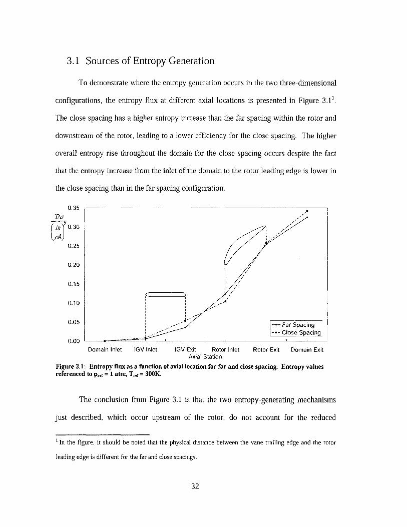
To demonstrate where the entropy generation occurs in the two three-dimensional
configurations, the entropy flux at different axial locations is presented in Figure 3.11.
The close spacing has a higher entropy increase than the far spacing within the rotor and
downstream of the rotor, leading to a lower efficiency for the close spacing. The higher
overall entropy rise throughout the domain for the close spacing occurs despite the fact
that the entropy increase from the inlet of the domain to the rotor leading edge is lower in
the close spacing than in the far spacing configuration.
0.35TAs
mjJ0.30
0.25
0.20
0.15
0.10
0.05 -+- Far Spacing--- Close Spacn
0.00Domain Inlet IGV Inlet IGV Exit Rotor Inlet Rotor Exit Domain Exit
Axial Station
Figure 3.1: Entropy flux as a function of axial location for far and close spacing. Entropy valuesreferenced to Pref = 1 atm, Tref = 300K.
The conclusion from Figure 3.1 is that the two entropy-generating mechanisms
just described, which occur upstream of the rotor, do not account for the reduced
1In the figure, it should be noted that the physical distance between the vane trailing edge and the rotor
leading edge is different for the far and close spacings.
32
performance in the close spacing. These two mechanisms imply that the additional
entropy generation in the close spacing occurs upstream of the rotor leading edge plane.
If so, the entropy flux into the rotor would have to be higher into the rotor in the close
spacing. This is not the case.
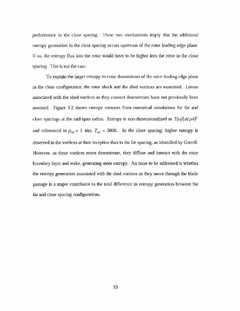
To explain the larger entropy increase downstream of the rotor leading edge plane
in the close configuration, the rotor shock and the shed vortices are examined. Losses
associated with the shed vortices as they convect downstream have not previously been
assessed. Figure 3.2 shows entropy contours from numerical simulations for far and
close spacings at the mid-span radius. Entropy is non-dimensionalized as TAs/(I /pA
and referenced to p,,f = 1 atm, T,,f = 300K. In the close spacing, higher entropy is
observed in the vortices at their inception than in the far spacing, as identified by Gorrell.
However, as these vortices move downstream, they diffuse and interact with the rotor
boundary layer and wake, generating more entropy. An issue to be addressed is whether
the entropy generation associated with the shed vortices as they move through the blade
passage is a major contributor to the total difference in entropy generation between the
far and close spacing configurations.
33
0.5
0.4
0.3
(a) (b)
Figure 3.2: Entropy contours at mid-span for (a) far spacing, (b) close spacing. All plots are of thesame scale. The lower contour plots correspond to the boxed regions in the upper plots, and have 20evenly-spaced intervals.
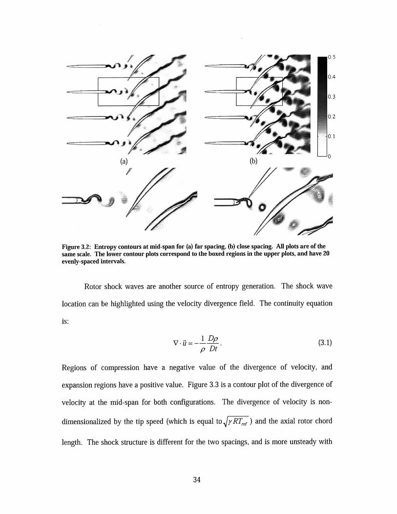
Rotor shock waves are another source of entropy generation. The shock wave
location can be highlighted using the velocity divergence field. The continuity equation
is:
V =- 1 p .(3.1)p Dt
Regions of compression have a negative value of the divergence of velocity, and
expansion regions have a positive value. Figure 3.3 is a contour plot of the divergence of
velocity at the mid-span for both configurations. The divergence of velocity is non-
dimensionalized by the tip speed (which is equal to RT,, ) and the axial rotor chord
length. The shock structure is different for the two spacings, and is more unsteady with
34
the close spacing compared to the far spacing. The entropy generation within the rotor
due to shock waves is quantified later in this chapter.
5
- 4
3
2
t30
-0
-2
4-3
~AW -4
(a) (b) -5
Figure 3.3: Divergence of velocity contours at mid-span for (a) far spacing, (b) close spacing. Blue
regions describe regions of compression, and red describe regions of expansion.
3.2 Numerical Approach to Compute Dissipation
In this section, the numerical implementation of the equations to calculate the
local entropy generation will be described. The entropy increase within a specified
control volume is then quantified to determine where differences exist between the close
and far spacing configurations.
The rate of entropy change of a fluid particle is:
Ds 1 au. 1 a ( Tp -r. ' +--I k-. (3.2)
Dt T a x, T ax, ax,
The two terms on the right-hand side of equation (3.2) represents entropy changes due to
viscous effects and heat transfer, respectively. The former is irreversible, but the latter
includes both reversible and irreversible changes. All irreversible processes in this thesis
will be referred to as dissipative processes, where entropy generation is equivalent to lost
35
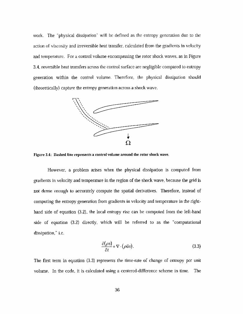
work. The "physical dissipation" will be defined as the entropy generation due to the
action of viscosity and irreversible heat transfer, calculated from the gradients in velocity
and temperature. For a control volume encompassing the rotor shock waves, as in Figure
3.4, reversible heat transfers across the control surface are negligible compared to entropy
generation within the control volume. Therefore, the physical dissipation should
(theoretically) capture the entropy generation across a shock wave.
Figure 3.4: Dashed line represents a control volume around the rotor shock wave.
However, a problem arises when the physical dissipation is computed from
gradients in velocity and temperature in the region of the shock wave, because the grid is
not dense enough to accurately compute the spatial derivatives. Therefore, instead of
computing the entropy generation from gradients in velocity and temperature in the right-
hand side of equation (3.2), the local entropy rise can be computed from the left-hand
side of equation (3.2) directly, which will be referred to as the "computational
dissipation," i.e.
a(Ps) +V -(pis). (3.3)at
The first term in equation (3.3) represents the time-rate of change of entropy per unit
volume. In the code, it is calculated using a centered-difference scheme in time. The
36
second term represents the net entropy flux for each computational cell. This is
computed by interpolating fluid properties to each cell boundary to define the net entropy
flux out of the cell volume at every instant in time.
The computational dissipation allows adequate evaluation of entropy generation
in regions with shock waves because the entropy is calculated from primitive variables,
which are obtained by solving the conservation equations in the Turbo simulation. In the
Turbo code, the numerical scheme includes additional dissipation, other than the physical
dissipation to accurately calculate entropy generation. This additional dissipation is
referred to as "numerical dissipation." The total dissipation (or entropy generation) is
therefore equal to the physical dissipation (computed from the gradients in velocity and
temperature) plus the numerical dissipation (implemented by the code). As the grid mesh
size goes to zero, the numerical dissipation also vanishes.
Using the new definitions for the calculated dissipation, the computational
dissipation is equal to the sum of the physical dissipation, numerical dissipation, and the
entropy changes due to reversible heat transfers across the control surface. As stated
previously, these reversible heat transfers are negligible in the region of shock waves.
They are identically zero if the bounding surface of the control volume of interest is
adiabatic.
The computational dissipation, when time-averaged and integrated over a
specified control volume, is equal to the time-averaged net entropy flux out of that
control volume. This is because the first term in equation (3.3) vanishes due to
periodicity of the flow field, i.e.:
S (ps)+V (PDs) dtdV= fJ(pDs). h dAdt. (3.4)I ff t
37
When the computational dissipation is integrated over a control volume with an adiabatic
surface, the computational dissipation should equal the entropy generation for that
volume.
Where heat transfer terms are negligible, the computational dissipation should
always be positive. Negative values, however, arise because the computational
dissipation is calculated using a centered-difference scheme as opposed to the up-winding
scheme used by Turbo. Entropy-generating flow features (e.g. shock waves, vortices) are
associated with both positive and negative values of the computational dissipation that
are located close together in the region of the flow feature. When the computational
dissipation is integrated over a control volume that encompasses both the positive and
negative values of the computational dissipation associated with these flow features, the
entropy generation is accurately captured.
The contribution of the physical dissipation and the computational dissipation can
be assessed independently in regions that have both shock waves and shear layers. This
allows us to determine how well the physical dissipation represents the actual entropy
rise for a control volume. Figure 3.5 shows the entropy rise within a control volume
defined from the vane trailing edge to a specified axial location and from hub to tip (these
are adiabatic surfaces). Within the first 40% of the axial gap, which is the region in
which the shed vortices are formed, the computational and physical dissipation are in
good agreement, implying that the physical dissipation accurately captures the entropy
generation associated with shear layers. After this point, the two dissipation schemes
diverge, and the physical dissipation under-estimates the computational (i.e. actual)
entropy flux. The divergence occurs because closer to the rotor, the shock wave is
38
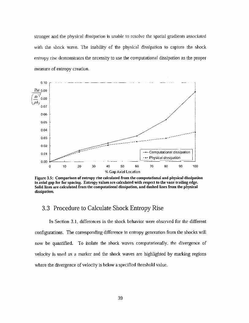
stronger and the physical dissipation is unable to resolve the spatial gradients associated
with the shock wave. The inability of the physical dissipation to capture the shock
entropy rise demonstrates the necessity to use the computational dissipation as the proper
measure of entropy creation.
0 .10 - - - - - -.-.--.
TAso.09-
0.08
0.07
0.06
0.05
0.04
0.02
0.01 'Computational dissipation
-- Physical dissipation0.00
0 10 20 30 40 50 60 70 80 90 100
% Gap Axial Location
Figure 3.5: Comparison of entropy rise calculated from the computational and physical dissipationin axial gap for far spacing. Entropy values are calculated with respect to the vane trailing edge.Solid lines are calculated from the computational dissipation, and dashed lines from the physicaldissipation.
3.3 Procedure to Calculate Shock Entropy Rise
In Section 3.1, differences in the shock behavior were observed for the different
configurations. The corresponding difference in entropy generation from the shocks will
now be quantified. To isolate the shock waves computationally, the divergence of
velocity is used as a marker and the shock waves are highlighted by marking regions
where the divergence of velocity is below a specified threshold value.
39
(a)
(b)
/
7
77
7/
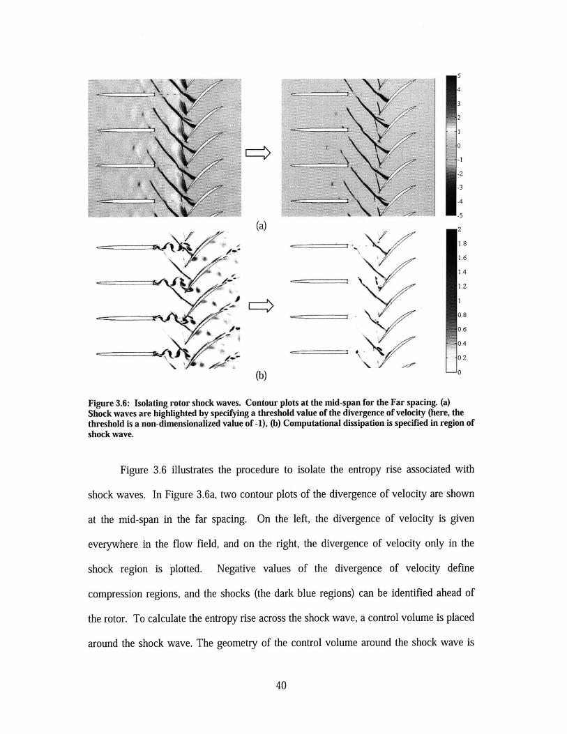
Figure 3.6: Isolating rotor shock waves. Contour plots at the mid-span for the Far spacing. (a)Shock waves are highlighted by specifying a threshold value of the divergence of velocity (here, thethreshold is a non-dimensionalized value of -1), (b) Computational dissipation is specified in region ofshock wave.
Figure 3.6 illustrates the procedure to isolate the entropy rise associated with
shock waves. In Figure 3.6a, two contour plots of the divergence of velocity are shown
at the mid-span in the far spacing. On the left, the divergence of velocity is given
everywhere in the flow field, and on the right, the divergence of velocity only in the
shock region is plotted. Negative values of the divergence of velocity define
compression regions, and the shocks (the dark blue regions) can be identified ahead of
the rotor. To calculate the entropy rise across the shock wave, a control volume is placed
around the shock wave. The geometry of the control volume around the shock wave is
40
determined by specifying a threshold value for the divergence of velocity. If the
divergence of velocity is below the threshold value at any cell, that cell is specified as
part of the shock wave control volume.
Implementing the above procedure of identifying the shock region is referred to as
"masking", because the shock waves are essentially masked from the rest of the flow
field. In Figure 3.6b, positive values of the computational dissipation are plotted in the
contour plot on the left. Negative values were not plotted because they would reduce the
clarity of the figure, but are immediately adjacent to regions where the computational
dissipation is positive. Negative values are important when integrating the computational
dissipation to find the entropy rise associated with the shock wave, as stated in Section
3.2. The computational dissipation is non-dimensionalized as T(comp. dissip.) cjp(/pA),
where comp. dissip. represents the quantity in equation (3.3). By applying the mask of
the divergence of velocity, the computational dissipation in the shock region is isolated,
as seen in the contour plot on the right of Figure 3.6b. Integrating the "masked"
computational dissipation in space and time gives the entropy rise associated with the
rotor shock.
- secondary mask
- primary mask
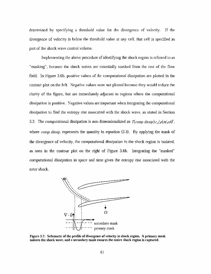
Figure 3.7: Schematic of the profile of divergence of velocity in shock region. A primary maskisolates the shock wave, and a secondary mask ensures the entire shock region is captured.
41
One issue in this procedure concerns setting the magnitude of the threshold. The
shock wave encompasses a finite region within which the divergence of velocity can take
on a range of values below the threshold value, as depicted in Figure 3.7. The choice of
threshold value is critical. If it is too high, it can include cells associated with flow
features unrelated to the shock. Therefore, a primary threshold value (called the primary
mask) is used to identify the general location of the shock, and then a secondary threshold
value (called the secondary mask) is applied to the immediate surroundings to ensure
capture of the entire shock region. If the divergence of velocity is below the secondary
threshold in the cells that neighbor the region where the primary mask is valid, those cells
are also considered to be in the shock region. This ensures that the complete shock
structure, and only the shock structure, is included in the mask and reduces numerical
error when the primary mask does not capture the entire shock region.
To apply the above procedure, three parameters must be specified: the primary
and secondary threshold values, and the number of neighboring cells around the cell
where the primary mask is valid to evaluate the secondary mask value. The values for all
three parameters, chosen to capture the entire shock region at all spans, were varied to
test sensitivity of the results. It was found that the value of each of the three parameters
does not change the conclusion that the majority of the differences in entropy generation
between configurations is not from shock waves. Table 3.1 shows the results from four
values of the primary mask that were used to compare the contribution from inside and
outside the masked region to the overall difference in rotor entropy rise between the far
and close configurations. To encompass the entire shock region for all values of the
42
primary mask in Table 3.1, the secondary mask was chosen to be -0.2, and was evaluated
within a range of two cells around the primary mask.
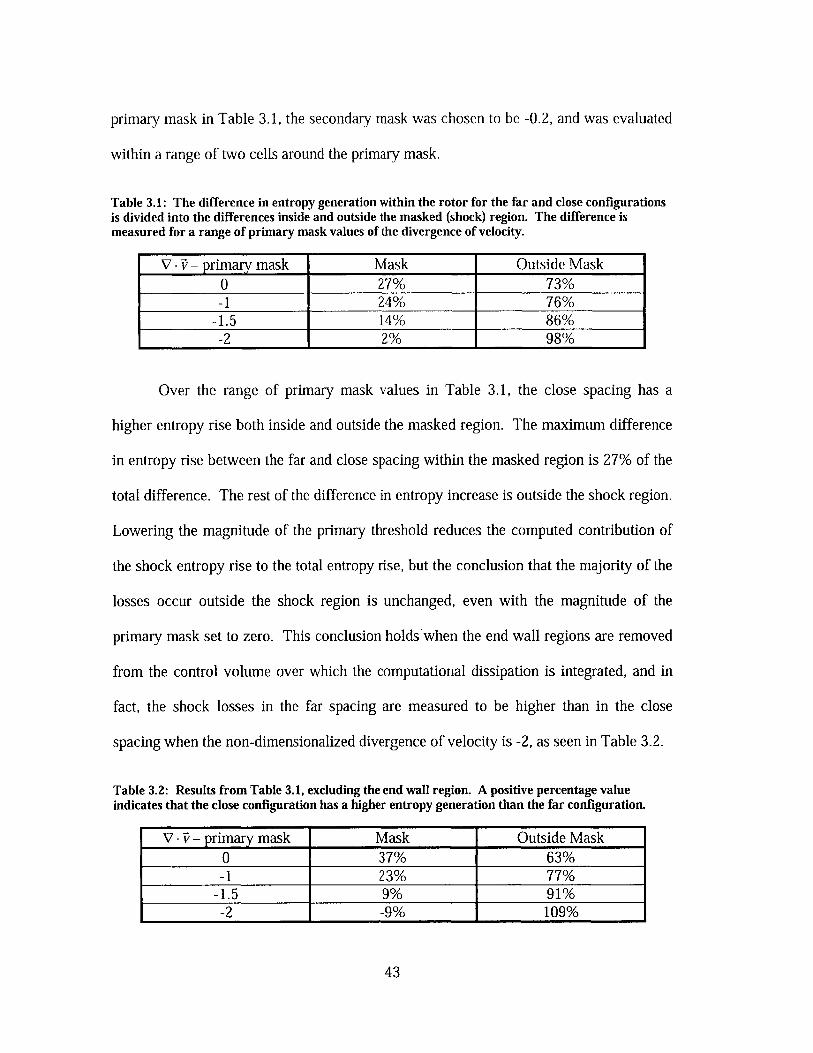
Table 3.1: The difference in entropy generation within the rotor for the far and close configurationsis divided into the differences inside and outside the masked (shock) region. The difference ismeasured for a range of primary mask values of the divergence of velocity.
V -v - primary mask Mask Outside Mask0 27% 73%
-1 24% 76%-1.5 14% 86%-2 2% 98%
Over the range of primary mask values in Table 3.1, the close spacing has a
higher entropy rise both inside and outside the masked region. The maximum difference
in entropy rise between the far and close spacing within the masked region is 27% of the
total difference. The rest of the difference in entropy increase is outside the shock region.
Lowering the magnitude of the primary threshold reduces the computed contribution of
the shock entropy rise to the total entropy rise, but the conclusion that the majority of the
losses occur outside the shock region is unchanged, even with the magnitude of the
primary mask set to zero. This conclusion holds when the end wall regions are removed
from the control volume over which the computational dissipation is integrated, and in
fact, the shock losses in the far spacing are measured to be higher than in the close
spacing when the non-dimensionalized divergence of velocity is -2, as seen in Table 3.2.
Table 3.2: Results from Table 3.1, excluding the end wall region. A positive percentage valueindicates that the close configuration has a higher entropy generation than the far configuration.
V. V- primary mask Mask Outside Mask0 37% 63%-1 23% 77%
-1.5 9% 91%-2 -9% 109%
43
The conclusion is that the entropy generation due to shock waves is not the
dominant mechanism responsible for the performance difference observed with changes
in spacing. The main difference between the far and close spacing configurations must
therefore be associated with differences in entropy generation from the vortices within
the rotor blade passage. The next chapter focuses on these shed vortices and their effect
on the overall stage performance as they propagate through, and interact with, the rotor.
44
Chapter 4
Vortex Trajectory within the Rotor
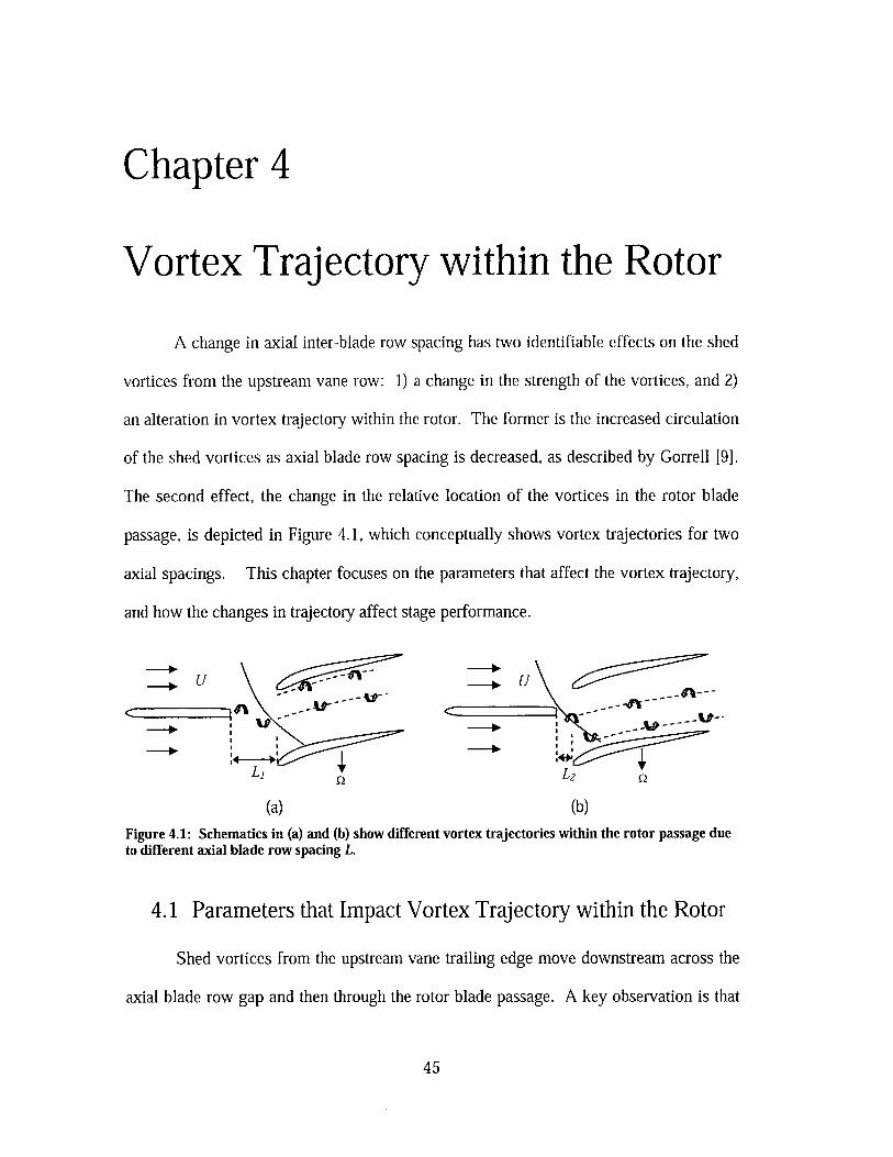
A change in axial inter-blade row spacing has two identifiable effects on the shed
vortices from the upstream vane row: 1) a change in the strength of the vortices, and 2)
an alteration in vortex trajectory within the rotor. The former is the increased circulation
of the shed vortices as axial blade row spacing is decreased, as described by Gorrell [9].
The second effect, the change in the relative location of the vortices in the rotor blade
passage, is depicted in Figure 4.1, which conceptually shows vortex trajectories for two
axial spacings. This chapter focuses on the parameters that affect the vortex trajectory,
and how the changes in trajectory affect stage performance.
U- U
(a) (b)
Figure 4.1: Schematics in (a) and (b) show different vortex trajectories within the rotor passage dueto different axial blade row spacing L.
4.1 Parameters that Impact Vortex Trajectory within the Rotor
Shed vortices from the upstream vane trailing edge move downstream across the
axial blade row gap and then through the rotor blade passage. A key observation is that
45
the pitch-wise location of the vortices within the rotor passage is defined by the pitch-
wise location of the vortex when it crosses the rotor leading edge plane. For a given
Mach number and blade geometry in this two-dimensional flow, the pitch-wise location
of the vortices is a function of the ratio between two times scales: the time it takes for a
vortex to travel the length of the vane-rotor gap, and one rotor period (i.e. the time for the
rotor to move one rotor pitch). To elaborate, let the time origin, t=O, be the instant the
vortex is shed. At this instant, the rotor is at a certain position with respect to the
upstream vane row. As the vortex travels the gap, the rotor moves from its position at
t=Q. Therefore, the relative location of the vortex in the rotor thus depends on how far
the rotor has rotated in the time it takes for the vortex to travel the length of the gap.
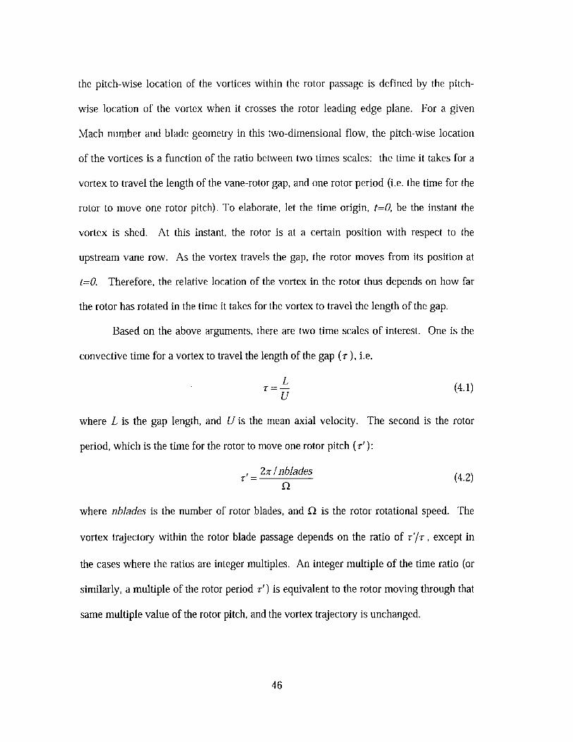
Based on the above arguments, there are two time scales of interest. One is the
convective time for a vortex to travel the length of the gap (r ), i.e.
LL =(4.1)U
where L is the gap length, and U is the mean axial velocity. The second is the rotor
period, which is the time for the rotor to move one rotor pitch (,'):
2z / nbladesQ' (4.2)
where nblades is the number of rotor blades, and n is the rotor rotational speed. The
vortex trajectory within the rotor blade passage depends on the ratio of r'/v, except in
the cases where the ratios are integer multiples. An integer multiple of the time ratio (or
similarly, a multiple of the rotor period r') is equivalent to the rotor moving through that
same multiple value of the rotor pitch, and the vortex trajectory is unchanged.
46
It should be emphasized that the vortex shedding from the upstream vane row is
directly linked to the rotor blade passing frequency by the rotor pressure field. More
specifically, the kinematics of the rotor shock impinging on the upstream vane row
dictate that the vortex shedding from the vane trailing edge occurs at a frequency equal to
the rotor blade passing frequency. The consequence of this relationship is that the rotor is
at the same relative position to the upstream vane row when vortices of the same sign are
shed.
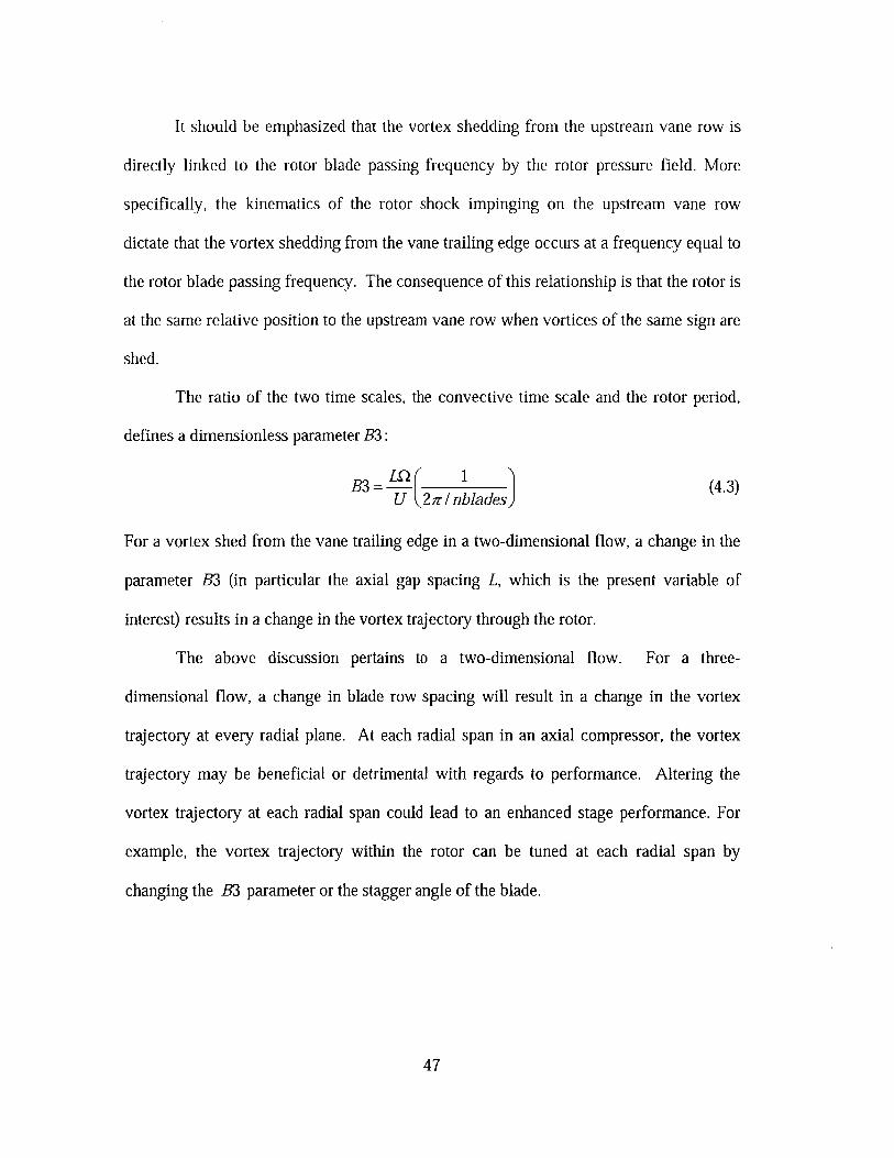
The ratio of the two time scales, the convective time scale and the rotor period,
defines a dimensionless parameter B3:
B3= -- (21/nbades (4.3)
For a vortex shed from the vane trailing edge in a two-dimensional flow, a change in the
parameter B3 (in particular the axial gap spacing L, which is the present variable of
interest) results in a change in the vortex trajectory through the rotor.
The above discussion pertains to a two-dimensional flow. For a three-
dimensional flow, a change in blade row spacing will result in a change in the vortex
trajectory at every radial plane. At each radial span in an axial compressor, the vortex
trajectory may be beneficial or detrimental with regards to performance. Altering the
vortex trajectory at each radial span could lead to an enhanced stage performance. For
example, the vortex trajectory within the rotor can be tuned at each radial span by
changing the B3 parameter or the stagger angle of the blade.
47
4.2 Vortex Trajectories in the Two-dimensional Computations
To assess the effect of a change in the vortex trajectory on rotor performance,
two-dimensional calculations have been conducted, as outlined in chapter two. The
configurations tested, referred to as "close2D" and "far2D," had axial blade row spacings
of 0.81 and 0.91 of the chord length, respectively. The value of B3 for close2D is 16.7
and for far2D is 18.8. At the same vane inlet corrected mass flow, close2D experiences a
3% decrease in work input and a 1.7% lower stagnation pressure ratio compared to far2D.
The efficiency at the rotor trailing edge is 0.01 points lower in close2D compared to far2D,
however, close2D iS 0.3 points lower far downstream.
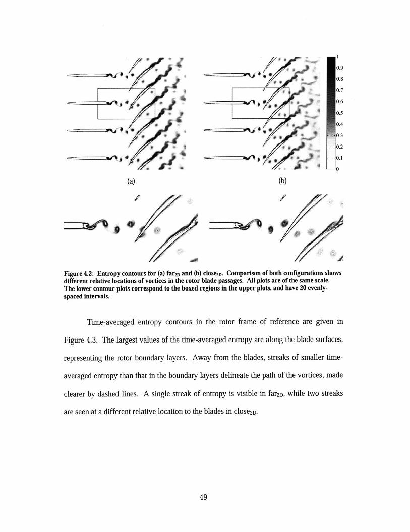
These changes can be linked to the different vortex trajectories within the rotor
passages for the two configurations, as pictured in the entropy contours of Figure 4.2.
For far2D, a clockwise vortex enters the mid-passage of the rotor, while a counter-
clockwise vortex intersects the rotor leading edge and remains near the blade. For
close2D, both vortices move through the rotor but are away from the blades.
48
( 4
(a) (b)
1
0.9
0.8
0.7
0.6
0.5
0.4
0.3
0.2
0
Figure 4.2: Entropy contours for (a) far2D and (b) closeZD- Comparison of both configurations showsdifferent relative locations of vortices in the rotor blade passages. All plots are of the same scale.The lower contour plots correspond to the boxed regions in the upper plots, and have 20 evenly-spaced intervals.
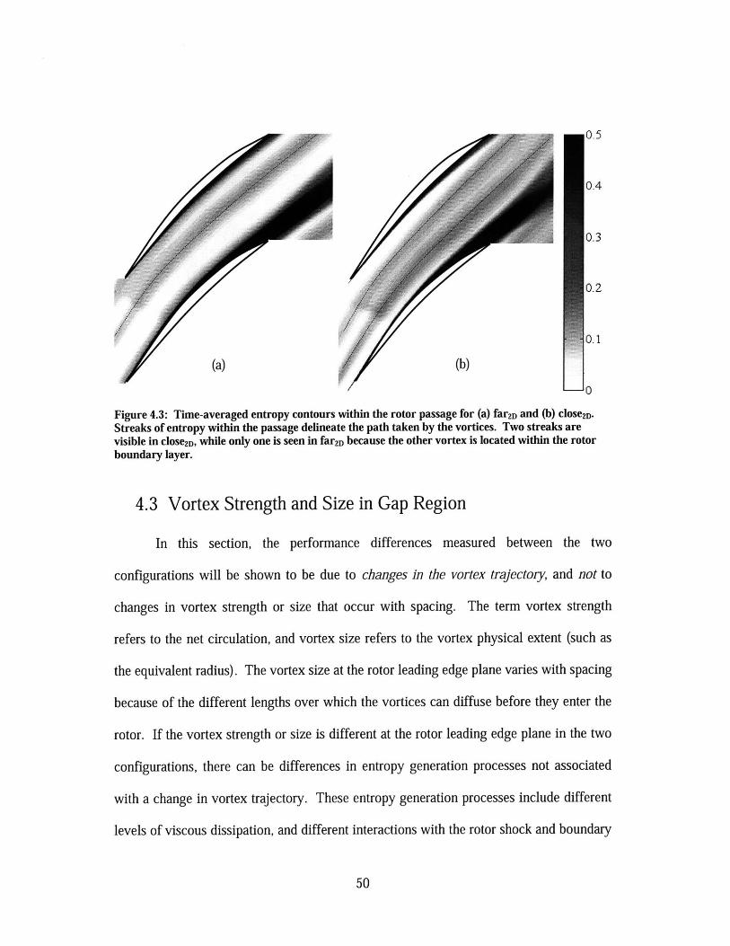
Time-averaged entropy contours in the rotor frame of reference are given in
Figure 4.3. The largest values of the time-averaged entropy are along the blade surfaces,
representing the rotor boundary layers. Away from the blades, streaks of smaller time-
averaged entropy than that in the boundary layers delineate the path of the vortices, made
clearer by dashed lines. A single streak of entropy is visible in far2D, while two streaks
are seen at a different relative location to the blades in close2D.
49
0.5
/ /0.3
0.2
(a) (b)
0
Figure 4.3: Time-averaged entropy contours within the rotor passage for (a) far2D and (b) close2D-Streaks of entropy within the passage delineate the path taken by the vortices. Two streaks arevisible in close2D, while only one is seen in far2D because the other vortex is located within the rotorboundary layer.
4.3 Vortex Strength and Size in Gap Region
In this section, the performance differences measured between the two
configurations will be shown to be due to changes in the vortex trajectory, and not to
changes in vortex strength or size that occur with spacing. The term vortex strength
refers to the net circulation, and vortex size refers to the vortex physical extent (such as
the equivalent radius). The vortex size at the rotor leading edge plane varies with spacing
because of the different lengths over which the vortices can diffuse before they enter the
rotor. If the vortex strength or size is different at the rotor leading edge plane in the two
configurations, there can be differences in entropy generation processes not associated
with a change in vortex trajectory. These entropy generation processes include different
levels of viscous dissipation, and different interactions with the rotor shock and boundary
50
layer (e.g. a vortex of larger circulation and size can influence the velocity field more
strongly). It is shown below that differences in vortex circulation and size are negligible
between the two configurations.
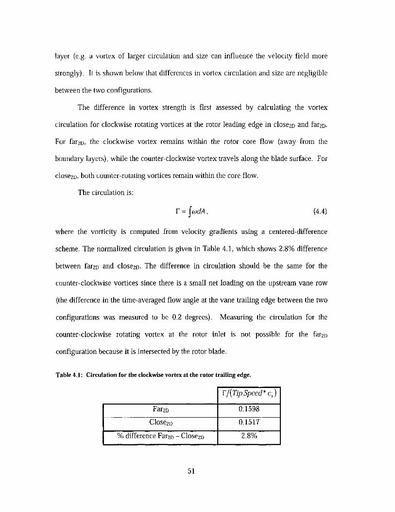
The difference in vortex strength is first assessed by calculating the vortex
circulation for clockwise rotating vortices at the rotor leading edge in close2D and far2D.
For far2D, the clockwise vortex remains within the rotor core flow (away from the
boundary layers), while the counter-clockwise vortex travels along the blade surface. For
close2D, both counter-rotating vortices remain within the core flow.
The circulation is:
F = JcodA, (4.4)
where the vorticity is computed from velocity gradients using a centered-difference
scheme. The normalized circulation is given in Table 4.1, which shows 2.8% difference
between far2D and close2D. The difference in circulation should be the same for the
counter-clockwise vortices since there is a small net loading on the upstream vane row
(the difference in the time-averaged flow angle at the vane trailing edge between the two
configurations was measured to be 0.2 degrees). Measuring the circulation for the
counter-clockwise rotating vortex at the rotor inlet is not possible for the far2D
configuration because it is intersected by the rotor blade.
Table 4.1: Circulation for the clockwise vortex at the rotor trailing edge.
F/(Tip Speed* cx)
Far2D 0.1598
Close2D 0.1517
% difference Far2D - Close2D 2.8%
51
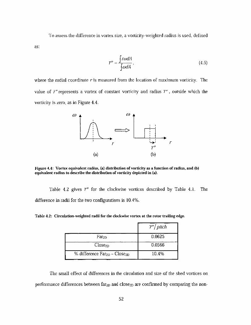
To assess the difference in vortex size, a vorticity-weighted radius is used, defined
as:
rcodA
fcodA
where the radial coordinate r is measured from the location of maximum vorticity. The
value of ' represents a vortex of constant vorticity and radius T', outside which the
vorticity is zero, as in Figure 4.4.
(4.5)
r -b)
(b)(a)
r
Figure 4.4: Vortex equivalent radius, (a) distribution of vorticity as a function of radius, and (b)equivalent radius to describe the distribution of vorticity depicted in (a).
Table 4.2 gives T' for the clockwise vortices described by Table 4.1.
difference in radii for the two configurations is 10.4%.
Table 4.2: Circulation-weighted radii for the clockwise vortex at the rotor trailing edge.
Vo/pitch
Far2D 0.0625
Close2D 0.0566
% difference Far2D - Close2D 10.4%
The
The small effect of differences in the circulation and size of the shed vortices on
performance differences between far2D and close2D are confirmed by comparing the non-
52
uniformity in the velocity field at the rotor leading edge. A measure of the non-
uniformity at any given plane is the quantity:
1 Y2PU , (4.6)2
where u' is defined as:
U'P = (U, - , + (u, - -aj (4.7)
The overbar represents the time- and pitch-wise area- average of the velocity component.
With no pressure variations within the flow, the quantity in (4.6) represents the potential
for stagnation pressure loss in an incompressible flow, as derived in Appendix A. In the
case of interest, there are pitch-wise non-uniformities in the velocity due to the rotor
pressure field, but the pressure field is assumed to change the non-uniformity metric by
the same magnitude in both configurations.
The non-uniformity metric, averaged over the pitch and in time, and non-
dimensionalized by the dynamic head at the inlet is:
ipu'z p U'dA dt2
- . (4.8)Ptiniet - Pmniet Ptiniet - Pinjet
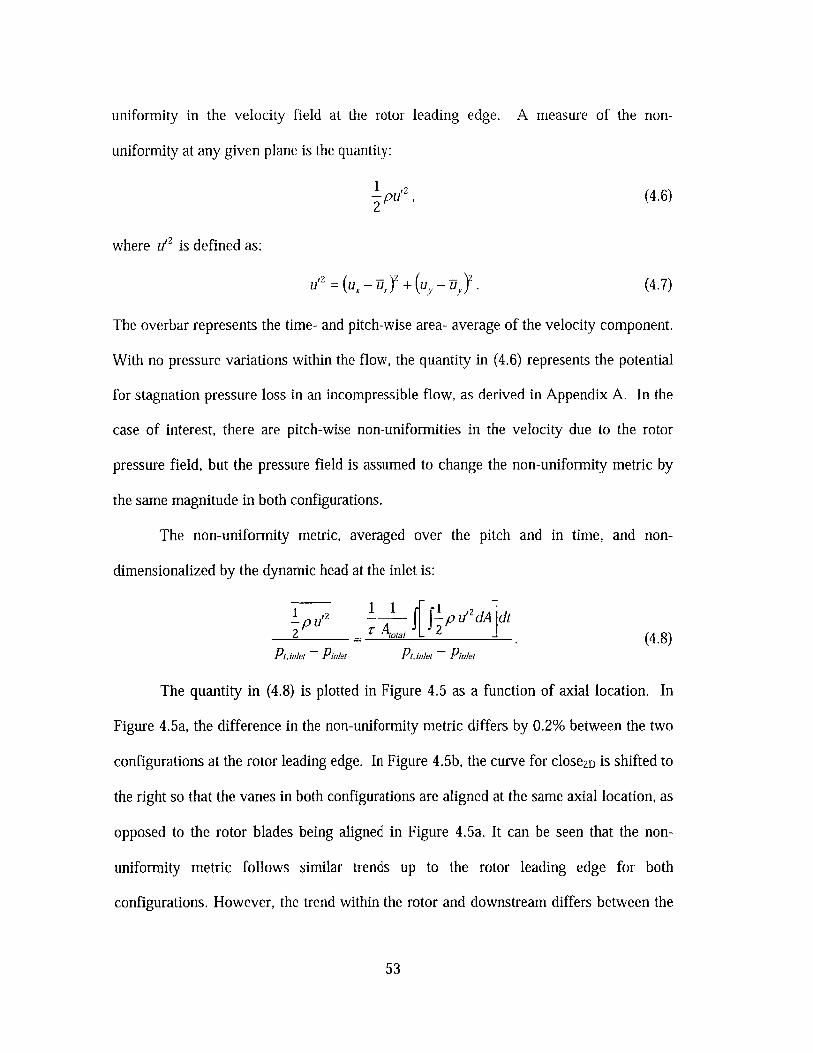
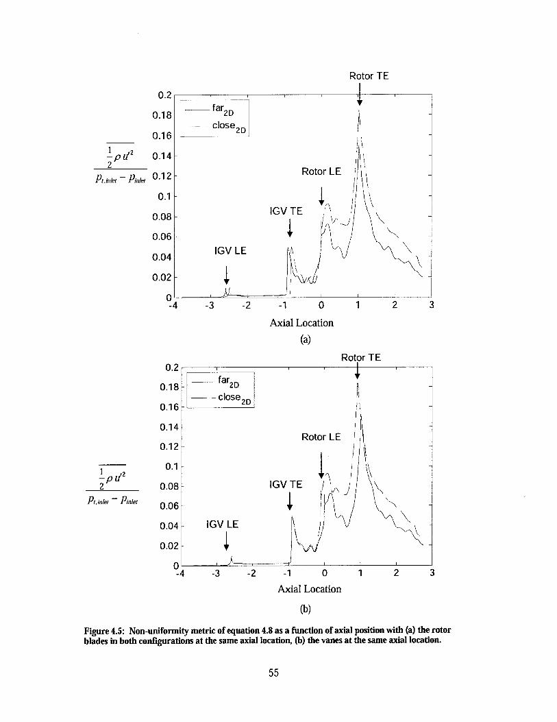
The quantity in (4.8) is plotted in Figure 4.5 as a function of axial location. In
Figure 4.5a, the difference in the non-uniformity metric differs by 0.2% between the two
configurations at the rotor leading edge. In Figure 4.5b, the curve for close2D is shifted to
the right so that the vanes in both configurations are aligned at the same axial location, as
opposed to the rotor blades being aligned in Figure 4.5a. It can be seen that the non-
uniformity metric follows similar trends up to the rotor leading edge for both
configurations. However, the trend within the rotor and downstream differs between the
53

two configurations, indicating different flow fields within the rotor. The differences
within the rotor are due to the different vortex trajectories, since this is the only differing
flow feature entering the rotor. At the rotor trailing edge, the difference in the non-
uniformity metric between configurations is 23%, much greater than at the leading edge.
In summary, the rotor is subjected to a similar non-uniformity at the leading edge in both
configurations.
With a similar non-uniformity ahead of the rotor, the performance differences
between far2D and close2D can be linked to how the vortices are processed within the rotor,
due to their relative respective trajectories. This is discussed in the following section.
54
Rotor TE
0.2
0.18
0.16
2
Pt,inlet - Pinet
0.14
0.12
0.1 F
0.08 -
0.06-
0.04-
0.02 -
p U'2
2
Pt,inlet - Pinlet
0-4
OlE
0.1(
0.14
0.1;
0.1
0.OE
0.O6
0.04
0.02;
C
-3 -2 -1 0 1 2 3
Axial Location
(a)
Rotor TE
far2D-
- - close2D
Rotor LE
IGV TE
- IGV LE
-4 -3 -2 -1 0 1 2 3
Axial Location
(b)
Figure 4.5: Non-uniformity metric of equation 4.8 as a function of axial position with (a) the rotorblades in both configurations at the same axial location, (b) the vanes at the same axial location.
55
far2D
close2 D
Rotor LE
IGV TE
IGV LE
AL/
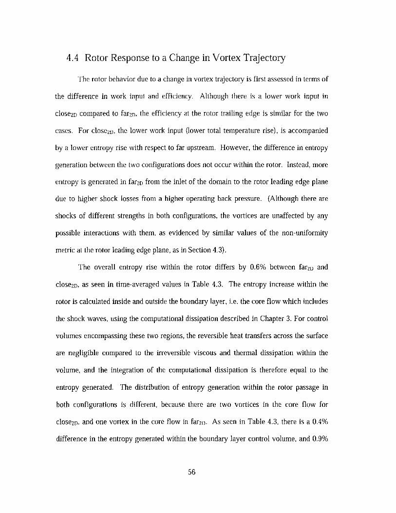
4.4 Rotor Response to a Change in Vortex Trajectory
The rotor behavior due to a change in vortex trajectory is first assessed in terms of
the difference in work input and efficiency. Although there is a lower work input in
close2D compared to far2D, the efficiency at the rotor trailing edge is similar for the two
cases. For close2D, the lower work input (lower total temperature rise), is accompanied
by a lower entropy rise with respect to far upstream. However, the difference in entropy
generation between the two configurations does not occur within the rotor. Instead, more
entropy is generated in far2D from the inlet of the domain to the rotor leading edge plane
due to higher shock losses from a higher operating back pressure. (Although there are
shocks of different strengths in both configurations, the vortices are unaffected by any
possible interactions with them, as evidenced by similar values of the non-uniformity
metric at the rotor leading edge plane, as in Section 4.3).
The overall entropy rise within the rotor differs by 0.6% between far2D and
close2D, as seen in time-averaged values in Table 4.3. The entropy increase within the
rotor is calculated inside and outside the boundary layer, i.e. the core flow which includes
the shock waves, using the computational dissipation described in Chapter 3. For control
volumes encompassing these two regions, the reversible heat transfers across the surface
are negligible compared to the irreversible viscous and thermal dissipation within the
volume, and the integration of the computational dissipation is therefore equal to the
entropy generated. The distribution of entropy generation within the rotor passage in
both configurations is different, because there are two vortices in the core flow for
close2D, and one vortex in the core flow in far2D. As seen in Table 4.3, there is a 0.4%
difference in the entropy generated within the boundary layer control volume, and 0.9%
56
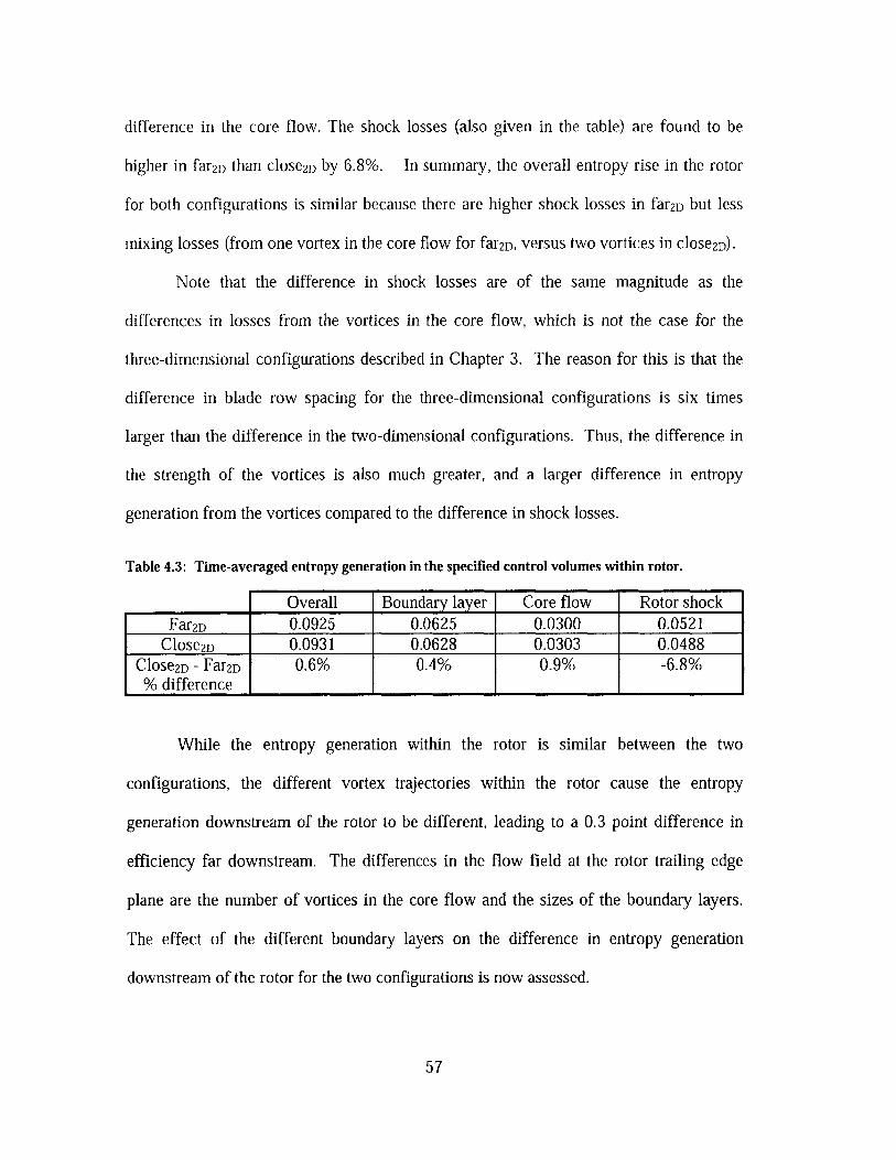
difference in the core flow. The shock losses (also given in the table) are found to be
higher in far2D than close2D by 6.8%. In summary, the overall entropy rise in the rotor
for both configurations is similar because there are higher shock losses in far2D but less
mixing losses (from one vortex in the core flow for far2D, versus two vortices in close2D).
Note that the difference in shock losses are of the same magnitude as the
differences in losses from the vortices in the core flow, which is not the case for the
three-dimensional configurations described in Chapter 3. The reason for this is that the
difference in blade row spacing for the three-dimensional configurations is six times
larger than the difference in the two-dimensional configurations. Thus, the difference in
the strength of the vortices is also much greater, and a larger difference in entropy
generation from the vortices compared to the difference in shock losses.
Table 4.3: Time-averaged entropy generation in the specified control volumes within rotor.
Overall Boundary layer Core flow Rotor shockFar2D 0.0925 0.0625 0.0300 0.0521
Close2D 0.0931 0.0628 0.0303 0.0488Close2D - Far2D 0.6% 0.4% 0.9% -6.8%% difference IIIII
While the entropy generation within the rotor is similar between the two
configurations, the different vortex trajectories within the rotor cause the entropy
generation downstream of the rotor to be different, leading to a 0.3 point difference in
efficiency far downstream. The differences in the flow field at the rotor trailing edge
plane are the number of vortices in the core flow and the sizes of the boundary layers.
The effect of the different boundary layers on the difference in entropy generation
downstream of the rotor for the two configurations is now assessed.
57
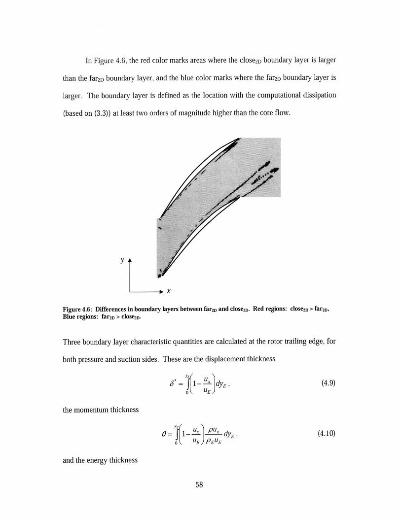
In Figure 4.6, the red color marks areas where the close2D boundary layer is larger
than the far2D boundary layer, and the blue color marks where the far2D boundary layer is
larger. The boundary layer is defined as the location with the computational dissipation
(based on (3.3)) at least two orders of magnitude higher than the core flow.
Y/
y
10x
Figure 4.6: Differences in boundary layers between far2D and close2D. Red regions: close2D > far2D,Blue regions: far2D > close2D-
Three boundary layer characteristic quantities are calculated at the rotor trailing edge, for
both pressure and suction sides. These are the displacement thickness
(4.9)
the momentum thickness
6= 1J- U Pux dyEUE PE UE
(4.10)
and the energy thickness
58
3* = 1-) dyE '0 E
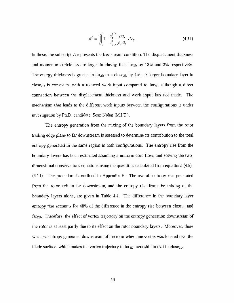
0E PEU
In these, the subscript E represents the free stream condition. The displacement thickness
and momentum thickness are larger in close2D than far2D by 13% and 3% respectively.
The energy thickness is greater in far2D than close2D by 4%. A larger boundary layer in
close2D is consistent with a reduced work input compared to far2D, although a direct
connection between the displacement thickness and work input has not made. The
mechanism that leads to the different work inputs between the configurations is under
investigation by Ph.D. candidate, Sean Nolan (M.I.T.).
The entropy generation from the mixing of the boundary layers from the rotor
trailing edge plane to far downstream is assessed to determine its contribution to the total
entropy generated in the same region in both configurations. The entropy rise from the
boundary layers has been estimated assuming a uniform core flow, and solving the two-
dimensional conservations equations using the quantities calculated from equations (4.9)-
(4.11). The procedure is outlined in Appendix B. The overall entropy rise generated
from the rotor exit to far downstream, and the entropy rise from the mixing of the
boundary layers alone, are given in Table 4.4. The difference in the boundary layer
entropy rise accounts for 40% of the difference in the entropy rise between close2D and
far2D. Therefore, the effect of vortex trajectory on the entropy generation downstream of
the rotor is at least partly due to its effect on the rotor boundary layers. Moreover, there
was less entropy generated downstream of the rotor when one vortex was located near the
blade surface, which makes the vortex trajectory in far2D favorable to that in close2D.
59
Table 4.4: Entropy rise from rotor trailing edge to far downstream.
Overall Boundary LayerClose2D 0.0568 0.0233
Far2D 0.0489 0.0203Difference (Close2D-Far2D) 0.0078 0.0030
The remaining difference in the entropy rise measured far downstream must be
due to the mixing and diffusion to a final uniform state of two vortices in the core flow
for close2D versus one vortex for far2D. The difficulty in measuring the entropy generation
from the vortices directly from the 2D simulations is isolating them from the rest of the
flow field. Downstream of the rotor trailing edge, the rotor boundary layer and vortices
mix together so that isolating the vortex at each instant in time while following it
downstream becomes difficult. Further, a defining characteristic associated with the
vortices was not obvious, since these characteristics were also associated with other parts
of the flow field (for example, using vorticity to mark the vortices would also capture
regions of the rotor boundary layer). Marking the fluid particles associated with the
vortices from their inception at the vane trailing edge is also difficult. Future work is thus
suggested to conclusively demonstrate that the mixing of the vortices in the core flow
accounts for the remaining difference in entropy generation.
4.5 Chapter 4 Summary
This chapter describes the impact of vortex trajectory within a rotor on its
performance. Two configurations are studied which have an axial spacing between the
vane and rotor that differ by 11%. The change in blade row spacing results in two
different vortex trajectories within the rotor. In one, there are two vortices in the passage
60

core flow. In the other, one vortex is within the passage core flow, and the other travels
along the surface of the blade.
It is found that the configuration with two vortices in the core flow has a lower
work input and lower efficiency. The difference in the rotor performance is attributed to
the difference in vortex trajectory through arguments that the flow non-uniformity ahead
of the rotor is similar for both spacings. Roughly 40% of the difference in the
downstream efficiency is attributed to a difference in the boundary layer at the rotor
trailing edge.
61
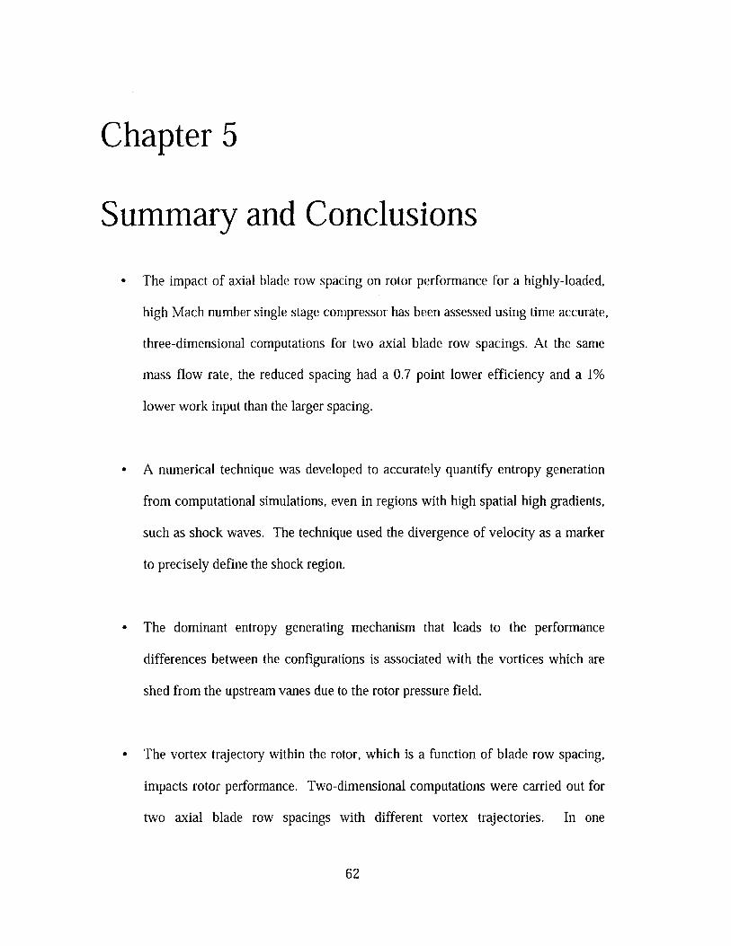
Chapter 5
Summary and Conclusions
- The impact of axial blade row spacing on rotor performance for a highly-loaded,
high Mach number single stage compressor has been assessed using time accurate,
three-dimensional computations for two axial blade row spacings. At the same
mass flow rate, the reduced spacing had a 0.7 point lower efficiency and a 1%
lower work input than the larger spacing.
- A numerical technique was developed to accurately quantify entropy generation
from computational simulations, even in regions with high spatial high gradients,
such as shock waves. The technique used the divergence of velocity as a marker
to precisely define the shock region.
- The dominant entropy generating mechanism that leads to the performance
differences between the configurations is associated with the vortices which are
shed from the upstream vanes due to the rotor pressure field.
- The vortex trajectory within the rotor, which is a function of blade row spacing,
impacts rotor performance. Two-dimensional computations were carried out for
two axial blade row spacings with different vortex trajectories. In one
62
configuration, one shed vortex was located within the boundary layer and one
outside the boundary layer (in the core flow). In the other configuration, both
vortices were located in the core flow. The latter configuration had a 3% lower
work input and a 0.3 point difference in efficiency, as measured far downstream
of the rotor.
- For a two-dimensional geometry at a given Mach number, the vortex trajectory is
found to be a function of the ratio between the convective time scale for the
vortices to travel the length of the axial gap between the vane and rotor blade
rows, and the rotor period (i.e. the time for a rotor to move one rotor pitch).
- The largest difference in the entropy generation between the two configurations
investigated occurred downstream of the rotor trailing edge. This is due to
different mixing processes that result from differences in the rotor boundary layer
and the different number of the vortices located in the core flow.
63
Chapter 6
Suggested Future Work
At the end of Chapter 4, future work was suggested to quantify the entropy generation
associated with the shed vortices downstream of the rotor trailing edge. This is
mentioned here again to reiterate that by using a different approach to calculate the
differences in entropy generation from the number of vortices, the boundary layer
calculations could also be verified and supported. The calculation of the entropy rise
from the mixing of the boundary layers downstream of the rotor invokes the assumption
that the flow field outside of the boundary layer is uniform. The impact of this
assumption has not been assessed in the mixing calculations outlined in Appendix B.
Also to be assessed is the impact of change in blade row spacing on the vortex
trajectory within the rotor, at each radial span, for a three-dimensional flow. A change in
vortex trajectory at each radial plane may be detrimental or beneficial to the overall
performance. The two-dimensional description of the effect of vortex trajectory on
performance, as presented in this thesis, is applicable at each radial plane if three
dimensional effects are unimportant. Recent work by Turner et al [20] suggests that
radial migration of high entropy fluid from the tip region impacts the radial profile of loss
downstream of the rotor. The relative importance of a change in vortex trajectory with
64

respect to other three-dimensional flow mechanisms that effect rotor performance as
blade row spacing is varied has yet to be determined.
As suggested at the end of Section 1.2, a blade row spacing may exist that
optimizes performance, due to competing effects of a change in vortex trajectory and
change in vortex strength with changes in blade row spacing. An investigation into this
idea is suggested for future work.
65
References
[1] Hetherington, R., and Moritz, R.R., 1976. "Influence of Unsteady FlowPhenomena on the Design and Operation of Aero Engines," AGARD Conf. Proc.,on Unsteady Flow Phenomena in Turbomachinery, 177.
[2] Smith L.H., Jr., 1970. "Casing Boundary Layers in Multistage Axial FlowCompressors," Flow Research in Blading, ed. L.S. Dzung, Elsevier PublishingCompany, Amsterdam.
[3] Mikolajczak, A.A., 1976. "The Practical Importance of Unsteady Flow," AGARDConf. Proc., on Unsteady Flow Phenomena in Turbomachinery, 177.
[4] Valkov, T.V., and Tan, C.S., 1999. "Effects of Upstream Rotor VorticalDisturbances on Time-Averaged Performance of Axial Compressor Stators: Part1- Framework of Technical Approach and Wake-Stator Blade Interactions," and"Part 2- Rotor Tip Vortex/Streamwise Vortex-Stator Blade Interactions," ASME J.Turbomachinery, 121(3), pp. 377-396.
[5] Sirakov, B.T., and Tan, C.S., 2003. "Effect of Unsteady Stator Wake - RotorDouble-Leakage Tip Clearance Flow Interaction on Time-Average CompressorPerformance," ASME Journal of Turbomachinery, 125(3), pp. 465-474.
[6] Gorrell, S.E., Okiishi, T.H., and Copenhaver, W.W., 2003. "Stator-RotorInteractions in a Transonic Compressor, Part 1: Effect of Blade-Row Spacing onPerformance," ASME Journal of Turbomachinery, 125(2), pp. 328-335.
[7] Chen, J.P., and Briley, W.R., 2001. "A Parallel Flow Solver for UnsteadyMultiple blade Row Turbomachinery Simulations.]," ASME Paper 2001-GT-348.
[8] Gorrell, S.E., Okiishi, T.H., and Copenhaver, W.W., 2003. "Stator-RotorInteractions in a Transonic Compressor, Part 2: Description of a Loss-ProducingMechanism," ASME Journal of Turbomachinery, 125(2), pp. 336-345.
[9] Gorrell, S.E., Car, D., Puterbaugh, S.L., Estevadeordal, J., and Okiishi, T.H., 2005."An Investigation of Wake-Shock Interactions in a Transonic Compressor WithDigital Particle Image Velocimetry and Time-Accurate Computational FluidDynamics," ASME Journal of Turbomachinery, 128(4), pp. 616-626.
[10] Morfey, C.L., and Fisher, M.J., 1970. "Shock-wave Radiation from a SupersonicDucted Rotor," Aeronautical Journal, Royal Aeronautical Society, 74(715), pp.579-585.
66
[11] Zachial, A. and Nurnberger, D., 2003. "A Numerical Study on the Influence ofVane-Blade Spacing on a Compressor Stage at Sub- and Trasonic OperatingConditions," ASME Paper GT2003-38020.
[121 Erdos, J.I., Alzner, E., and McNally W., 1997. "Numerical Solution of PeriodicTransonic Flow through a Fan Stage," AIAA Journal, 15(11), pp. 1559-1568.
[131 Chen, J.P., Celestina M.L., and Adamczyk J.J., 1994. "A New Procedure forSimulating Unsteady Flows through Turbomachinery Blade Passage," ASMEPaper 94-G T-151.
[14] Chen J.P., and Barter, J.W., 1998. "Comparison of Time-Accurate Calculationsfor the Unsteady Interaction in Turbomachinery Stage," AIAA-98-3292.
[15] Wang, X.,and Chen, J.P., 2004. "A Post-Processor to Render TurbomachineryFlows Using Phase-Lag Simulations," AIAA-2004-615, 42nd AIAA AerospaceSciences Meeting and Exhibit, pp. 5997-6003.
[16] Villanueva, A.V., 2006. "Characterization of the Flow Field Response toVaneless Space Reduction in Centrifugal Compressors," M.Sc. Thesis,Department of Mechanical Engineering, Massachusetts Institute of Technology.
[17] Gorrell, S.E., Personal communication, U.S. Air Force Research Laboratory,Wright Patterson Air Force Base, Ohio.
[18] Chriss, R.M., Copenhaver, W.W., and Gorrell, S.E., 1999. "The Effects of Blade-Row Spacing on the Flow Capacity of a Transonic Rotor," ASME Paper 99-GT-209.
[19] Beach, T., 2003. Personal communication with Gorrell, S.E., AP Solutions.
[201 Turner, M.G., Gorrell, S.E., and Car, D., 2005. "Radial Migration of ShedVortices in a Transonic Rotor Following a Wake Generator: A ComparisonBetween Time Accurate and Average Passage Approach," ASME Paper GT2005-68776.
[21] Gorrell, S.E., 2001. "An Experimental and Numerical Investigation of Stator-Rotor Interactions in a Transonic Compressor," Ph.D. Dissertation, Department ofMechanical Engineering, Iowa State University.
67
Appendix A
Non-uniformity Metric
In Chapter 4, a metric to measure the degree of non-uniformity ahead of the rotor
was defined as:
21p '2 (4.6)2
where u'2 is a perturbation velocity, defined as:
U'f2 = (U" -U)2 + (U,-,. (4.7)
The overbar represents the time- and pitch-wise area- average of the velocity component.
The non-uniformity metric is averaged over the pitch and in time, and non-
dimensionalized by the dynamic head at the inlet. Its mathematical form is:
1 P u'2 1 U2dA-dt
2 Aj_ L A",., . (4.8)Ptniet - Pinlet Pinlet - Pinlet
The averaged quantity in (4.8) will now be shown to be a suitable metric to define the
non-uniformity in the flow field. This is first shown by demonstrating that the non-
uniformity metric represents the pressure difference between two axial planes by using
the conservation of momentum (however, the factor of 1/2 does not appear). Using linear
momentum, the non-uniformity in the flow field can be shown to act as a blockage that
decreases the flow area, and hence, reduces the pressure. The non-uniformity can also be
68
related to the stagnation pressure losses if the flow at an axial location was allowed to
mix to a uniform state.
First, linear momentum is used to determine how non-uniformity affects pressure
changes in a flow. The impulse function is written as:
I=p+pu2 . (A.1)
The impulse function, when integrated across the inlet and exit flow area (planes 'a' and
'b') of a specified control volume, is the same if there are no forces acting on the control
volume and there is no change in area. Steady flow is assumed. Mathematically, this is
stated as:
AI= Ib -, =0 (A.2)
The overbar in this equation, and in the rest of this section, represents the pitch-wise or
area-average of the impulse function. Pressure and velocity at any point can be defined
as the sum of its average quantity on the plane of interest, plus its spatially-varying
quantity:
p=p p' (A.3)
U=U+U' (A.4)
Note that the area-average of the spatially-varying component of the pressure and
velocity are zero, i.e. p' = 0 and u' = 0.
Substituting the expressions of A.3 and A.4 into the impulse function:
I= p+pf'+ p(a2 + 2u'+ u' 2) (A.4)
69
By assuming the density and cross-sectional area remains constant, the continuity
equation simplifies to: ua =Ub. The difference in the momentum between planes 'a' and
'b' is:
AI =Pb ,-p+ 2-p(Ut -u' )+ p(U2 U2) (A.5)
Area-averaging the impulse function gives:
II=~ 2)-p,+p'zz= 0 (A.6)AlI=PbJ + P Ub (_.U)
The difference in pressure from planes 'a' to 'b' is therefore related to the non-uniformity
at both stations by rearranging (A.6):
,2 _U -PU 2(A.7)Pb PUb aPA
If at plane 'b', the flow is fully mixed out, then:
P Pa - pua (A.8)
The term on the right-hand side of A.8 is similar to the non-uniformity metric, and
therefore indicates that the metric represents the pressure rise that would be obtained if
the non-uniformity was allowed to mix to a uniform state. Therefore, the non-uniformity
represents a blockage in the flow area, which tends to reduce pressure.
The term included in the non-uniformity metric appears when considering the
difference in mass-averaged stagnation pressure differences between planes 'a' and 'b'.
The stagnation pressure for incompressible flow is given as:
1 = P+-pu2 (A.9) 2
The stagnation pressure can be multiplied by the velocity and averaged across the pitch to
find a velocity-weighted average value for the stagnation pressure. This is equivalent to
multiplying the stagnation pressure by the local mass flux and finding a mass-averaged
70
stagnation pressure. However, the density is not included when multiplying by the mass
flux because the density is assumed constant, and therefore is not required when
comparing two axial locations. The velocity-weighted stagnation pressure is written as:
up, = up+-pu3
2(A.10)
Substituting the expressions for pressure and velocity from (A.3) and (A.4) into (A.10):
up, = Up +up' + + Up +u'IP' + I p(3 +3M2 'U' +u' 32
(A.11)
A pitch-wise average of (A. 11) gives:
p up 1 -3up, = up +U'P' +- pH B
23 _-1 --puu +-pu'32 2
The difference in mass-averaged stagnation pressure between planes 'a' and 'b' becomes
(by also applying the continuity equation):
3 -Aup, = UAp+Au'p'+-piuAu'2
21 -
+-pAu'32(A.13)
Using the pressure difference from conservation of linear momentum given in (A.7), the
first term on the left-hand side of (A.13) can be replaced:
Aup, = u pAu2 )+ Aup'+-pUA u'2 +-pA u'2 2
(A.14)
which reduces to:
A ru1 1Aup, = Au'+-UAU'2 +-pAu' 3
2 2(A.15)
For a non-uniform flow that does not have large variations in the velocity profile, the
approximation iIAu2 >> Au' 3 is valid. Furthermore, for one-dimensional shear flow,
p'= 0 . The expression in (A.15) becomes:
71
(A.12)
A up, = { -pA u' (A.16)
Therefore, the non-uniformity metric at any plane represents the potential for stagnation
pressure losses if the flow at that axial location was allowed to mix to a uniform state in a
constant area duct. The assumptions include incompressible, one-dimensional flow,
which makes the use of the non-uniformity metric approximate.
Finally, the non-uniformity metric also represents the difference between the area-
averaged stagnation pressure and the stagnation pressure based on the average quantities
on an axial plane. The latter stagnation pressure is given as:
- 1 -p= +-p 2 (A.17)2
An area-average of the stagnation pressure pf is (since area-average of u'and p'are
zero):
A =+ Up&2 +U' 2 (A.18)Pt -
And the difference between (A.17) and (A.18) also leads to the expression of the non-
uniformity metric:
S- p 1 2 (A.19)t A -P22
In summary, the non-uniformity metric calculated in (4.8) at any axial plane of
interest represents a number of physical quantities: the blockage at that location, the
potential for stagnation pressure losses, and the difference in the area-averaged stagnation
pressure compared to the stagnation pressure compared from the average values of
pressure and velocity at that location. All three physical scenarios are an indication of the
level of non-uniformity at a specified location.
72
The analysis of the present section assumed that the flow non-uniformity was
constant in time. However, since the flow field at any axial location is unsteady, the non-
uniformity metric is adjusted by computing the perturbation velocity given in (4.7) with
respect to the time- and pitch-wise average of the velocity component. This makes the
non-uniformity metric an approximation, but nonetheless provides a suitable quantity
when comparing similar flow fields for the two configurations under study in Chapter 4.
73
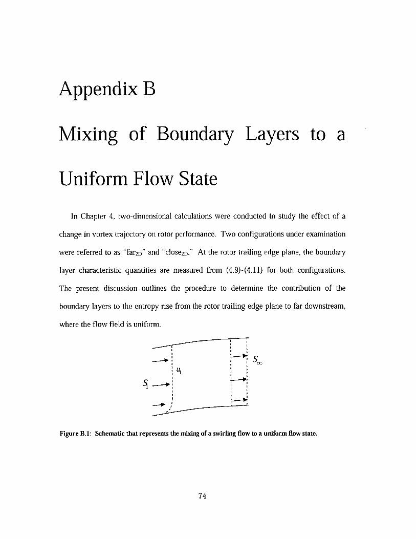
Appendix B
Mixing of Boundary Layers to a
Uniform Flow State
In Chapter 4, two-dimensional calculations were conducted to study the effect of a
change in vortex trajectory on rotor performance. Two configurations under examination
were referred to as "far2D" and "close2D." At the rotor trailing edge plane, the boundary
layer characteristic quantities are measured from (4.9)-(4.11) for both configurations.
The present discussion outlines the procedure to determine the contribution of the
boundary layers to the entropy rise from the rotor trailing edge plane to far downstream,
where the flow field is uniform.
~,
Figure B.1: Schematic that represents the mixing of a swirling flow to a uniform flow state.
74
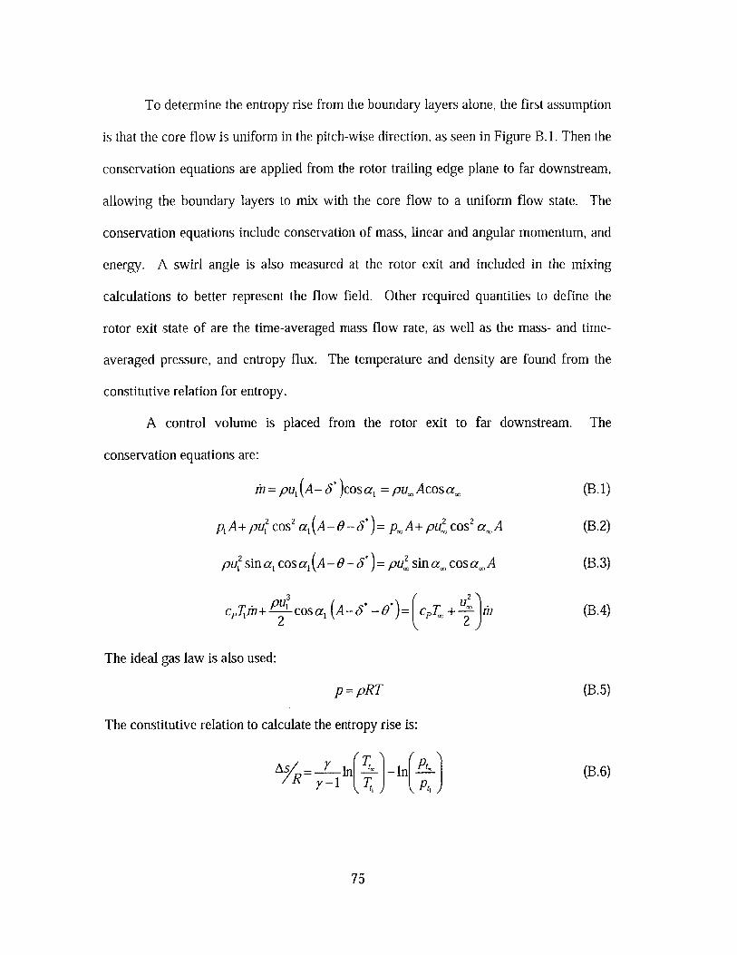
To determine the entropy rise from the boundary layers alone, the first assumption
is that the core flow is uniform in the pitch-wise direction, as seen in Figure B. 1. Then the
conservation equations are applied from the rotor trailing edge plane to far downstream,
allowing the boundary layers to mix with the core flow to a uniform flow state. The
conservation equations include conservation of mass, linear and angular momentum, and
energy. A swirl angle is also measured at the rotor exit and included in the mixing
calculations to better represent the flow field. Other required quantities to define the
rotor exit state of are the time-averaged mass flow rate, as well as the mass- and time-
averaged pressure, and entropy flux. The temperature and density are found from the
constitutive relation for entropy.
A control volume is placed from the rotor exit to far downstream. The
conservation equations are:
= pu (A-,5*)cosal = puAcosa, (B. 1)
p1A+pu2 cos 2 a,(A -0 -3* )= p, A+ pu cos' a. A (B.2)
pu, sin a, cosa,(A -- 3*)= pu2 sin a cos a A (B.3)
32
c , ;+ cos a, (A - * -0* = CPT + h (B.4)22
The ideal gas law is also used:
p= pRT (B.5)
The constitutive relation to calculate the entropy rise is:
As R In TL- ln (B.6)IR r_1 T Pt
75
From mass conservation in (B. 1), the uniform core velocity, u,, can be found
since the mass flow rate is measured, and all other quantities are known. The values at
downstream infinity can then be determined by solving (B.1)-(B.5) simultaneously, and
the entropy rise calculated from (B.6).
The entropy increase from the rotor leading edge to downstream infinity was
independent of the value of the entropy flux at the rotor leading edge. There was a slight
dependence of the entropy rise due to mixing on pressure. Varying the pressure at the
rotor exit by 1.3% (which is the difference between the mass-averaged and area-averaged
pressure) caused the difference in entropy rise between the two configurations to change
by 2.5%. This difference in the entropy rise was not enough to change the conclusions
derived from the mixing calculation. The results of the mixing calculations are presented
in Table 4.4.
76