Impact of Uncertainty in Magnitude-Area Scaling Relations on SCEC Broadband Platform Simulations

Report for SCEC Award #15105 Submitted March 11, 2016

Investigators: Jeff Bayless, Dr. Andreas Skarlatoudis, and Dr. Paul Somerville (AECOM)

I. Project Overview .................................................................................................................................... iA. Abstract ............................................................................................................................................ iB. SCEC Annual Science Highlights ..................................................................................................... iC.Exemplary Figure ............................................................................................................................. iD.SCEC Science Priorities .................................................................................................................. iiE. Intellectual Merit .............................................................................................................................. iiF. Broader Impacts .............................................................................................................................. iiG.Project Publications ......................................................................................................................... ii

II. Technical Report ................................................................................................................................... 1A. Introduction ...................................................................................................................................... 1B. Objectives ........................................................................................................................................ 1C.Approach ......................................................................................................................................... 2

1. Simulation Events ..................................................................................................................... 3D.Results ............................................................................................................................................. 4E. Conclusions ..................................................................................................................................... 4F. References ...................................................................................................................................... 5G.Appendix A: Additional Figures ....................................................................................................... 6

i

I. Project Overview

A. Abstract In the box below, describe the project objectives, methodology, and results obtained and their signifi-cance. If this work is a continuation of a multi-year SCEC-funded project, please include major research findings for all previous years in the abstract. (Maximum 250 words.) There is an unresolved debate about the way in which the rupture areas of large crustal earthquakes scale with seismic moment. The SCEC Broadband Platform (BBP) provides the opportunity to study in detail the impact of using two different M-A scaling relations in simulations: Leonard (2010), which the BBP Phase 1 validation project used as a guideline for selecting fault areas (Dreger et al., 2013 and Goulet et al., 2015), and Hanks and Bakun (2008), which results in smaller fault rupture areas than Leonard (2010) for about M>6.7. In our evaluation we use the already-implemented simulation methods and rupture generators to study both previously validated events (Type A) and a suite of selected event scenarios (Type B). For Type A validations, we utilize the simulated waveforms computed from the BBP Phase 1 validation project (Dreger et al., 2013.) and results are evaluated using the bias of simulated RotD50 with respect to obser-vations (termed goodness of fit, or GOF). We re-compute the events of interest using the HB08 scaling relation to define the fault rupture area. For Type B validations, we study four event scenarios, repeating each using both M-A relations to define fault geometry. The results are dependent on the magnitude of the scenario (as expected) and vary between simulation methods. For Type A events, both the EXSIM and UCSB methods appear largely unaffected by the decrease in fault width associated with Hanks and Bakun (2008) scaling. For UCSB with the Type B scenarios, an increase in the average level of simulations is observed for the smaller fault areas. The SDSU and Graves and Pitarka methods behave similarly, which is to be expected at long periods. For Graves and Pitarka at short periods (<1 sec) the change to smaller fault area results in a slight decrease in the level of simulated motions. For Graves and Pitarka and SDSU at long periods (>1 sec) the change to smaller fault area results in an increase (up to about 30% for Landers and 20% for the M 7.0 scenario events) in the level of simulated motions. Based on communica-tions with the modelers, in general this behavior is as expected. We hope that quantifying the impact of two M-A scaling relations on four BBP simulation methods will provide guidance to the modelers for the simulation of future earthquake scenarios, in Phase 2 of the Validation effort, and in other forward simula-tions.

B. SCEC Annual Science Highlights Each year, the Science Planning Committee reviews and summarizes SCEC research accomplishments, and presents the results to the SCEC community and funding agencies. Rank (in order of preference) the sections in which you would like your project results to appear. Choose up to 3 working groups from be-low and re-order them according to your preference ranking.

Ground Motion Simulation Validation (GMSV) Ground Motion Prediction (GMP)

C. Exemplary Figure Select one figure from your project report that best exemplifies the significance of the results. The figure may be used in the SCEC Annual Science Highlights and chosen for the cover of the Annual Meeting Proceedings Volume. In the box below, enter the figure number from the project report, figure caption and figure credits.

Figure 5: Type A simulation - Landers event, GP simulation method.

ii

D. SCEC Science Priorities In the box below, please list (in rank order) the SCEC priorities this project has achieved. See https://www.scec.org/research/priorities for list of SCEC research priorities. For example: 6a, 6b, 6c

6, 6e

E. Intellectual Merit How does the project contribute to the overall intellectual merit of SCEC? For example: How does the research contribute to advancing knowledge and understanding in the field and, more specifically, SCEC research objectives? To what extent has the activity developed creative and original concepts?

This project’s objectives are directly related to the Ground-Motion prediction focus group and to refining phys-ics-based simulation methodologies. The behavior of magnitude-area scaling relations, especially for large mag-nitudes, is very significant and directly affects the simulated waveforms computed by the majority of the simula-tion methods currently implemented on the SCEC BBP. The results of this project a) quantify the differences and the impact of the different types of the magnitude-area scaling relations on the different simulation methods; b) provide to the modelers a tool with which to assess their models and refine the way in which they handle dif-ferent types of magnitude area scaling relations and c) provide a guide to the modelers for the simulation of fu-ture earthquake scenarios. The results will be shared with the Broadband Platform Validation Project and there-by facilitate the use of simulated waveforms for improved hazard representation.

F. Broader Impacts How does the project contribute to the broader impacts of SCEC as a whole? For example: How well has the activity promoted or supported teaching, training, and learning at your institution or across SCEC? If your project included a SCEC intern, what was his/her contribution? How has your project broadened the participation of underrepresented groups? To what extent has the project enhanced the infrastructure for research and education (e.g., facilities, instrumentation, networks, and partnerships)? What are some possible benefits of the activity to society?

This project has supported the already strong collaboration of the group of scientists who work on and for the SCEC broadband platform, by contributing to the research goals and interacting on a regular basis with scientists (and engineers.) Possible benefits of the activity to society involve the improvement of earthquake simulations, which will eventually be used in seismic design, particularly for near fault ground motions.

G. Project Publications All publications and presentations of the work funded must be entered in the SCEC Publications data-base. Log in at http://www.scec.org/user/login and select the Publications button to enter the SCEC Pubi-cations System. Please either (a) update a publication record you previously submitted or (b) add new publication record(s) as needed. If you have any problems, please email web@scec.org for assistance.

1

II. Technical Report

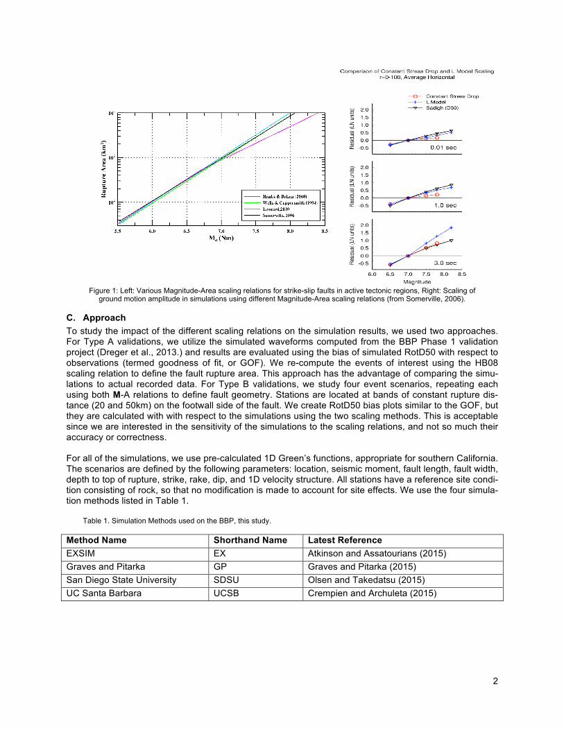
A. Introduction There is an unresolved debate about the way in which the rupture areas of large crustal earthquakes scale with seismic moment. This debate has its origins in Hanks and Bakun (2002; 2008) who proposed bilinear source-scaling relations to match the moment magnitude (M) - log(Area, A) observations of Wells and Coppersmith (1994). They built these relations assuming constant stress-drop scaling for M≤6.7 and a transition to non-self-similar scaling following the L-model (Scholz, 1982) scaling for M>6.7. In the L-model, the displacement, D, grows in proportion to the fault length, L, with increasing magnitude once fault width, W, reaches its maximum value. For large magnitudes, L-models have large displacements and small areas and do not have self-similar scaling of magnitude with area above the transition. In self-similar models (e.g. Leonard, 2010), average fault displacement, fault length and fault width all in-crease uniformly together. For example, self-similar scaling relations arise when the average displace-ment on a fault rupture surface changes at the same rate as its change in area, yielding constant stress drop. A comparison of the two different types of relations is shown in Figure 1 (left panel). The differences in magnitude estimates for a given fault rupture area from the different scaling models described above have a relatively minor impact on the estimation of ground motion amplitudes using em-pirical ground motion models. A change of 0.2 units in magnitude (a factor of 2 in seismic moment) results in a change of about 15% in ground motion level at a period of 3 seconds (Somerville, 2006). This is be-cause the empirical ground motion models implicitly account for the change in rupture area associated with the magnitude difference. However, for numerical waveform simulations in which the fault area is fixed, a change in 0.2 units in magnitude has a significant impact on the produced synthetic waveforms. This impact is dependent on the simulation method used, but Somerville (2006) has shown that at very long periods, this change is a factor of two, about six times that for empirical ground motion models. An example of this effect is shown in Figure 1 (right panel). This very large sensitivity of simulated ground motion amplitudes to scaling relations renders these relations a major issue for strong motion simulation; particularly at large magnitudes, where the simulations are of most interest to the engineering seismology community. The SCEC Broadband Platform (BBP) provides the opportunity to study in detail the impact of using two different M-A scaling relations in simulations: Leonard (2010), which the BBP Phase 1 validation project used as a guideline for selecting fault areas (Dreger et al., 2013 and Goulet et al., 2015), and Hanks and Bakun (2008), which results in smaller fault rupture areas than Leonard (2010) for about M>6.7. In our evaluation we use the already-implemented simulation methods and rupture generators to study both previously validated events (Type A) and a suite of selected event scenarios (Type B). In this report Leonard (2010) is abbreviated as L10, and Hanks and Bakun (2008) is abbreviated as HB08.

B. Objectives • Quantify the impact of two M-A scaling relations on four BBP simulation methods.

• Provide the modelers a tool with which to assess their models, and to refine the way in which they

handle different types of M-A scaling relations, or perhaps select them.

• Provide guidance to the modelers for the simulation of future earthquake scenarios, in Phase 2 of the Validation work, and in other forward simulations.

2

Figure 1: Left: Various Magnitude-Area scaling relations for strike-slip faults in active tectonic regions, Right: Scaling of

ground motion amplitude in simulations using different Magnitude-Area scaling relations (from Somerville, 2006).

C. Approach To study the impact of the different scaling relations on the simulation results, we used two approaches. For Type A validations, we utilize the simulated waveforms computed from the BBP Phase 1 validation project (Dreger et al., 2013.) and results are evaluated using the bias of simulated RotD50 with respect to observations (termed goodness of fit, or GOF). We re-compute the events of interest using the HB08 scaling relation to define the fault rupture area. This approach has the advantage of comparing the simu-lations to actual recorded data. For Type B validations, we study four event scenarios, repeating each using both M-A relations to define fault geometry. Stations are located at bands of constant rupture dis-tance (20 and 50km) on the footwall side of the fault. We create RotD50 bias plots similar to the GOF, but they are calculated with with respect to the simulations using the two scaling methods. This is acceptable since we are interested in the sensitivity of the simulations to the scaling relations, and not so much their accuracy or correctness. For all of the simulations, we use pre-calculated 1D Green’s functions, appropriate for southern California. The scenarios are defined by the following parameters: location, seismic moment, fault length, fault width, depth to top of rupture, strike, rake, dip, and 1D velocity structure. All stations have a reference site condi-tion consisting of rock, so that no modification is made to account for site effects. We use the four simula-tion methods listed in Table 1.

Table 1. Simulation Methods used on the BBP, this study.

Method Name Shorthand Name Latest Reference EXSIM EX Atkinson and Assatourians (2015) Graves and Pitarka GP Graves and Pitarka (2015) San Diego State University SDSU Olsen and Takedatsu (2015) UC Santa Barbara UCSB Crempien and Archuleta (2015)

3

1. Simulation Events The difference between the two types of scaling relations start at magnitudes M~6.7, so we limit our study to events with magnitudes M>6.6. The Type A validation events used in this study are the Loma Prieta (M 6.94), Northridge (M 6.73) and Landers (M 7.22) events. The Type B scenarios are M 6.6 strike slip, M 6.6 reverse, M 7.0 strike slip, and M 7.0 reverse scenarios. These events and scenarios are listed in Ta-ble 2, along with the corresponding rupture dimensions as used in the SCEC BBP version 15.3, the L10 scaling relation, and the HB08 scaling relation. The BBP Phase 1 validation project (Dreger et al., 2013 and Goulet et al., 2015) loosely based the fault dimensions on the L10 scaling relation (along with expert judgment and group consensus), as evidenced by Table 2. In order to utilize the results of that project, we have chosen to re-compute the events and scenarios listed below using the HB08 scaling relation. In determining the HB08 fault dimensions, we ac-commodate the smaller HB08 faults areas by keeping the fault length from the BBP v15.3 dimensions, and reducing the fault width (since W is relatively less constrained than L, personal communication with Rob Graves.) By making this selection, we may underestimate the effect the M-A scaling relation, be-cause this choice allows the overall rupture duration to remain unchanged. If we had reduced only the fault length, the energy would be concentrated in a shorter time window and the amplitudes would be in-creased, even in a stochastic method. Reducing both length and width would be intermediate between these two cases, and may be explored further in another study.

Table 2. Type A events and Type B scenarios, and their rupture dimensions, used in this study.

Type A used in BBP v15.3 Leonard (2010) Hanks & Bakun (2008)

Event M Area (km2)

L (km)

W (km)

Area (km2)

L (km)

W (km)

Area (km2)

L (from BBP)

W = A/L

Landers 7.22 1680 80 21 1698 77.19 22 1295.7 80 16.2

Northridge 6.73 540 20 27 537 20 26.85 555.9 20 27.8

Loma Prieta 6.94 880 40 22 891 46.17 19.3 798.8 40 20

Type B used in BBP v15.3 Leonard (2010) Hanks & Bakun (2008)

Scenario M Area (km2)

L (km)

W (km)

Area (km2)

L (km)

W (km)

Area (km2)

L (from BBP)

W = A/L

So Cal Strike Slip 6.6 397.6 28.2 14.1 407.4 28.9 14.1 416.9 28.2 14.8

So Cal Re-verse 6.6 397.6 28.2 14.1 398 25.95 15.34 416.9 28.2 14.8

So Cal Strike Slip 7.0 - - - 1023.3 50.2 20.4 886.1 50.2 17.65

So Cal Re-verse 7.0 - - - 1000 45.1 22.17 886.1 45.1 19.65

4

D. Results For the Type A events, we aggregate the results in GOF summary plots (averages of residuals over all simulation stations and hypocenter realizations) using the GP, EXSIM, and SDSU methods. In each panel of these summary plots, the top GOF is computed using simulations with Leonard (2010) M-A scaling, the second GOF is computed using using simulations with HB08 scaling, and the bottom curve shows the log- difference between the two, where positive values represent increased levels for the HB08 scaling simulations. For the Type B simulations, we aggregate the results in a similar manner. Since there are no recordings from which to calculate residuals, we instead take the following approach. At each station, we average the RotD50 at each period over the 50 source realizations, effectively getting the “average” spectrum for that site. This is done both for the HB08 and L10 simulations, and then the log-ratio of the average spec-tra are taken for each site. We perform the statistics on this quantity, and present the results in a similar plot to the Type A results. The complete set of comparison plots, for all four simulation methods, is included in this report; see Ap-pendix A. We have omitted the Northridge event, and the M 6.6 scenario comparison plots because they show negligible sensitivity to the scaling relation, as expected given their magnitude.

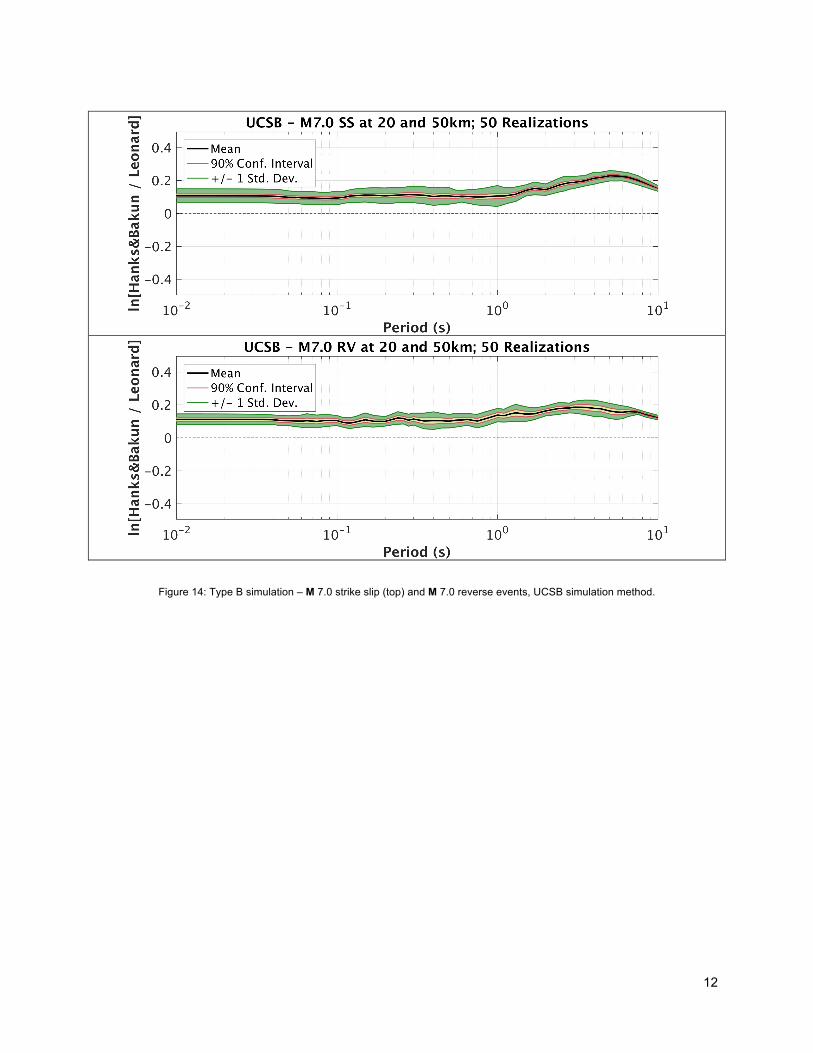
E. Conclusions This section summarizes the results with respect to the Loma Prieta (M 6.94) and Landers (M 7.22) events, and the M 7.0 strike slip, and M 7.0 reverse scenarios. See Appendix A for related plots. The EX method is largely unaffected by the decrease in fault width associated with HB08 scaling. This observation is consistent between the Type A simulations, and the Type B scenarios. We have contacted the developers of EX, and they both commented that these results are as expect for EX (Gail Atkinson and Karen Assatourians, pers. comm.). Specifically, Gail Atkinson noted “the main finite-fault effects in EXSIM are geometric (location of fault relative to stations).” Karen Assatourians specified “as long as the moment of the earthquake remains identical and seismic stations distances (or the average of distances) are not very short and in the range of source size, the source finiteness effects are not that significant.” For the UCSB method, the change to smaller fault areas results in a minor increase in the average level of simulations across all oscillator periods for the Loma Prieta event. The Landers event was not com-pleted in the BBP v15.3 simulations, so that comparison was not made. For the Type B scenarios, a larg-er increase in the average level of simulations is observed for the smaller fault areas, and this increase is consistent across all oscillator periods. The increase relative to the L10 simulations peaks at periods longer than 3 seconds, at about 20% increase. We have contacted the UCSB modelers to discuss possi-ble explanations for the substantial increase observed in the Type B scenarios, but not observed for Lo-ma Prieta. One explanation is the fact that Loma Prieta was modeled as a buried rupture (Ztor = 4km) and the Type B scenarios were modeled as surface ruptures. Another possibility is the velocity model; all Type B simulations were performed using Green’s functions generated from a southern CA model, and Loma Prieta was performed using Green’s functions generated from a northern CA model. The SDSU and GP methods behave similarly at long periods, which is expected since both methods use the same code for long periods. For GP, at short periods (<1 sec) the change to smaller fault area results in a slight decrease in the level of simulated motions. Based on communication with Rob Graves, this re-flects an attribute of the stochastic approach where the results can have a slight dependence on N*dl, where N is the total number of subfaults, and dl is the average subfault dimension. Since we have slightly reduced N, the product N*dl is smaller, resulting in the observed decrease in short period amplitudes. For the GP and SDSU methods, at long periods (>1 sec) the change to smaller fault area results in an increase (up to about 30% for Landers and 20% for the M 7.0 scenario events) in the level of simulated motions. Since the magnitude (and therefore seismic moment) is fixed for an event, decreasing the fault area requires that the average slip on the fault be increased. The increased fault slip is responsible for the observed increase in long period amplitudes.

5

F. References Atkinson, G. M., and K. Assatourians (2015). Implementation and validation of EXSIM (a stochastic finite-

fault ground-motion simulation algorithm, Seismol. Res. Lett. 86, no. 1, doi: 10.1785/0220140097. Crempien, J., and R. Archuleta (2015). UCSB method for broadband ground motion from kinematic simu-

lations of earthquakes, Seismol. Res. Lett. 86, no. 1, doi: 10.1785/0220140103. Dreger, Douglas S. (Chair), Gregory C. Beroza, Steven M. Day, Christine A. Goulet, Thomas H. Jordan,

Paul A. Spudich, and Jonathan P. Stewart (2013). Evaluation of SCEC Broadband Platform Phase 1 Ground Motion Simulation Results, Submitted August 1, 2013.

Goulet, C.A., Abrahamson, N.A., Somerville, P.G., and Wooddell, K.E. (2015) The SCEC Broadband Plat-form Validation Exercise: Methodology for Code Validation in the Context of Seismic-Hazard Analyses. Seismological Research Letters, January/February 2015, 86, p. 17-26, doi: 10.1785/0220140104

Graves, R.W. and A. Pitarka (2010). Broadband Ground-Motion Simulation Using a Hybrid Approach, Bull. Seism. Soc. Am., 100, 2095-2123, doi:10.1785/0120100057

Graves, R., and A. Pitarka (2015). Refinements to the Graves and Pitarka (2010) broadband ground mo-tion simulation method, Seismol. Res. Lett. 86, no. 1, doi: 10.1785/0220140101.

Hanks, T. C., and W. H. Bakun (2002). A bilinear source-scaling model for M-log(A) observations of con-tinental earthquakes, Bull. Seismol. Soc. Am., 92, 1841–1846.

Hanks, T. C., and W. H. Bakun (2008). M- log A Observations for Recent Large Earthquakes, Bull. Seis-mol. Soc. Am., 99, 490-494.

Leonard M., (2010). Earthquake Fault Scaling: Self-Consistent Relating of Rupture Length, Width, Aver-age Displacement, and Moment Release, Bull. Seism. Soc. Am., 100, 1971-1988, doi:10.1785/0120090189

Olsen, K., and R. Takedatsu (2015). The SDSU broadband ground motion generation module BBtoolbox Version 1.5, Seismol. Res. Lett. 86, no. 1, doi: 10.1785/0220140102.

Scholz, C. (1982). Scaling laws for large earthquakes and consequences for physical models, Bull. Seis-mol. Soc. Am., 72, 1–14.

Somerville, P. (2006). Review of magnitude-area scaling of crustal earthquakes, Rept. to WGCEP, URS Corp., Pasadena, 22 pp.

Wells, D. L., and K. J. Coppersmith (1994). New empirical relationships among magnitude, rupture length, rupture width, rupture area, and surface displacement, Bull. Seismol. Soc. Am., 84, 974–1002.

6

G. Appendix A: Additional Figures

Figure 2: Fault orientation (red line/plane) and station locations for M7.0 strike slip (top row) and M7.0 reverse (bottom row) scenario earthquakes. The left column shows fault dimensions and station location for the HB08 scaling, and the

right column shows those for L10 scaling.

1

Figure 3: Fault orientation and station location for the Landers (top) and Loma Prieta (bottom) simulations.

2

Figure 4: Type A simulation - Landers event, EX simulation method.

3

Figure 5: Type A simulation - Landers event, GP simulation method.

4

Figure 6: Type A simulation - Landers event, SDSU simulation method.

5

Figure 7: Type A simulation - Loma Prieta event, EX simulation method.

6

Figure 8: Type A simulation - Loma Prieta event, GP simulation method.

7

Figure 9: Type A simulation - Loma Prieta event, SDSU simulation method.

8

Figure 10: Type A simulation - Loma Prieta event, UCSB simulation method.

9

Figure 11: Type B simulation – M 7.0 strike slip (top) and M 7.0 reverse events, EX simulation method.

10

Figure 12: Type B simulation – M 7.0 strike slip (top) and M 7.0 reverse events, GP simulation method.

11

Figure 13: Type B simulation – M 7.0 strike slip (top) and M 7.0 reverse events, SDSU simulation method.

12

Figure 14: Type B simulation – M 7.0 strike slip (top) and M 7.0 reverse events, UCSB simulation method.