IMPACT OF UNCERTAIN INPUT ON PARAMETER …

IMPACT OF UNCERTAIN INPUT ON PARAMETER ESTIMATION

IN GROUNDWATER MODEL

BY

XIANG JI

THESIS

Submitted in partial fulfillment of the requirements

for the degree of Master of Science in Civil Engineering

in the Graduate College of the

University of Illinois at Urbana-Champaign, 2012

Urbana, Illinois

Adviser:

Professor Albert J. Valocchi

ii

ABSTRACT

Description of the aquifer characteristics accurately and efficiently is the most commonly

encountered and probably the most challenging aspect of groundwater modeling. In the context

of groundwater modeling, although many studies have focused on parameter estimation

problems, these issues are far from being solved. When important hydrogeological parameters

like transmissivity and storativity are estimated using regression-based inverse methods, it is

assumed that all other parameters and quantities are known. In particular, it is assumed that

pumping rates are known. This will not be a valid assumption for groundwater basins subject to

intensive irrigation pumping since farmers are normally not required to report their pumping

amounts to any government regulatory office. In this thesis, we study the impact of uncertainty

in pumping upon estimation of hydrogeological parameters. We use three typical simplified

groundwater models to test the impact of uncertain pumping on the parameter estimation and we

use statistical methods to assess the results.

The uncertainty analysis using the Matlab Regression Toolbox of the Thiem and Theis

model shows that the impact of uncertain drawdown is less than the impact of uncertain pumping.

The uncertainty analysis using PEST for a more complex model with a partially penetrating

stream shows that the stream depletion cannot be used to estimate the transmissivity and the

drawdown cannot be used to estimate the riverbed conductivity. The biases of estimated

parameters commonly exist and they increase with the increasing uncertainty of model input.

The impact of uncertain pumping rate is also more significant than the impact of uncertain

observations.

Finally, we estimate the pumping uncertainty in a real case by studying the data from the

Republican River Compact Administration (RRCA) model. In this unusual case, we have actual

metered pumping data, as well as an assumed pumping rate that was used in the RRCA model.

For the Upper Natural Resources District of Nebraska, the error (uncertainty) in pumping rates

approximately follows a Gaussian distribution. But the pumping rate used in the model is

underestimating the actual pumping data.

iii

ACKNOWLEDGMENTS

This project would not have been possible without the support of many people. Many

thanks go to my adviser, Albert J. Valocchi, who read my numerous revisions and helped me

make some sense of the confusion. Also thanks go to my group members, Professors Ximing Cai

and Nicholas Brozovic, and fellow graduate students Richeal Young, Yao Hu, Taro Mieno,

Tianfang Xu and Ruijie Zeng, who offered me guidance and support. I received partial financial

support for this study from the U.S. National Science Foundation, grant NSF EAR 07-09735.

And finally, thanks go to my family and numerous friends who endured this long process with

me, always offering support and love.

iv

TABLE OF CONTENT

Chapter 1 Introduction ......................................................................................................... 1

1.1 Motivation .................................................................................................................................... 1

1.2 Problem statement ...................................................................................................................... 1

1.3 Literature review ........................................................................................................................ 3

1.4 Research Objectives .................................................................................................................... 4

1.5 Overview ...................................................................................................................................... 5

Chapter 2 Methodology ........................................................................................................ 6

2.1 Introduction ................................................................................................................................. 6

2.2 The PEST Algorithm .................................................................................................................. 7

Chapter 3 Uncertainty Analysis in Two Typical Analytical Model ................................ 11

3.1 Steady-State Model (Thiem Equation) .................................................................................... 11

3.2 Transient Model (Theis Equation) .......................................................................................... 19

3.3 Comparison and Conclusion .................................................................................................... 29

Chapter 4 Uncertainty Analysis of Partially Penetrating Stream System Using PEST 30

4.1 Introduction ............................................................................................................................... 30

4.2 Mathematical Description ........................................................................................................ 30

4.3 Parameter Estimation Using PEST ......................................................................................... 32

4.4 Comparison and Conclusion .................................................................................................... 35

Chapter 5 Pumping Data Analysis in the Republican River Compact Administration

(RRCA) Groundwater Model .................................................................................................... 37

5.1 Introduction ............................................................................................................................... 37

5.2 Data Analysis ............................................................................................................................. 38

Chapter 6 Conclusions and Future Work ......................................................................... 40

6.1 Conclusions ................................................................................................................................ 40

6.2 Future Work .............................................................................................................................. 41

Chapter 7 Figures and Tables ............................................................................................ 43

Bibliography.... ............................................................................................................................ 95

1

Chapter 1 Introduction

1.1 Motivation

Watershed hydrology and groundwater models are important tools for water management

for both operational and research programs. The widespread application of groundwater models

is accompanied by a widespread concern about quantifying the uncertainties prevailing in their

use. Overestimation of uncertainty may lead to expenditures in time and money and overdesign

of watershed management infrastructure. Conversely, underestimation of uncertainty may lead to

poor designs that fail at an unacceptably high frequency, with potentially serious effects.

Much attention has been paid to uncertainty issues in hydrological modeling due to their

great effects on prediction and further on decision-making. Aleatory uncertainty is the inherent

variation in the natural system which is stochastic and irreducible. Epistemic uncertainty is

caused by the limitation of knowledge of the quantities or processes identified with the system

which is subjective and reducible (Ross, Ozbek and Pinder 2009). For example, the uncertainty

in field measurements is primarily aleatory while the uncertainty in forecasting behavior using

models is primarily epistemic. In general, epistemic uncertainties could be improved by

comparing and modifying the diverse model components (Hejberg and Refsgaard 2005).

Relatively, the uncertainty of input data and its impact on parameter estimation is more difficult

to deduce. Also, the parameter estimation is essential to assess the surface and/or sub-surface

water potential in any area, since we cannot measure the parameters directly. In this inverse

problem, not only is the uncertainty of observations (input data) non-negligible, but the model

structure is uncertain, so the uncertainty of estimated parameters is significant. Currently,

parameter estimation and uncertainty is a hot topic in the uncertainty research field (Sudheer,

Lakshmi and Chaubey 2010).

1.2 Problem statement

Description of the aquifer characteristics accurately and efficiently is the most commonly

encountered and probably the most challenging aspect of groundwater modeling. An accurate

description of an aquifer is crucial to effective groundwater management. The goal of

2

groundwater parameterization is to estimate the spatial distribution of the aquifer properties, e.g.,

transmissivity and storage. This is an inverse problem, and there are many mathematical

techniques available for this kind of problem (see section 1.3.2). However, the aquifer

characterization is non-unique and extremely difficult for many reasons. First of all,

transmissivity and storage are highly variable in space. It is impossible to obtain the complete

measurement of these parameters for a large area. Usually we use pumping test to estimate

average T and S over the whole region. Secondly, due the complex nature of the aquifer, we

generally use mathematical model to simulate the behavior of groundwater flow, so the

uncertainty of those parameters cannot be neglected. In addition, when we use regression based

approaches like PEST (which is an acronym for Parameter ESTimation) (Doherty 2010) or other

inverse methods to estimate hydrogeologic parameters, we assume that all other input parameters

(e.g., pumping rate) are known. Specifically, in this thesis, pumping data and drawdown

observations are required, which are also uncertain.

In general, the uncertainty of model input is caused by the changes in natural conditions,

limitation in measurement and lack of data (Beck 1987) . In particular, irrigation pumping data

are rarely available, even though they are the most important input data for regional groundwater

modeling in basins that are subject to intensive irrigation. In most cases, pumping rates are

estimated using information such as incomplete pumping records, crop water requirement data,

remotely sensed images and power usage records. Figure 1 is a representative example which

shows the estimated total amount of groundwater pumped from the Death Valley Regional

groundwater Flow System (DVRFS) model domain during the period 1913-98 (Moreo, et al.

2003). This large uncertainty shown in this figure is attributed to incomplete pumping records,

misidentification of crop type, and errors associated with estimating annual domestic

consumption, the irrigation area, and crop application rates. In many cases, the average pumping

rate is used and all analyses, including parameter estimation, ignore the large uncertainty in

pumping data.

In the context of groundwater modeling, although many studies have focused on parameter

estimation problems, these issues are far from being solved. In particular, prior studies have

neglected to account for the impact of input uncertainty, like that illustrated above in Figure 1,

upon parameter estimation. This is the overall motivation for this thesis.

3

1.3 Literature review

1.3.1 Groundwater modeling

In early groundwater models, the restrictive assumptions were made regarding the aquifer

shape and parameter variability in order to obtain analytical closed-form solutions. In the 1950s

and 1960s, U.S. Geological Survey (USGS) hydrologists and others took further advantage of

physical and mathematical analogies to create more realistic models of complex groundwater

systems. Along with the growth of mathematical theory and the increase in computer capability,

in 1960s and 1970s numerical models became widely used. These models use numerical

approximation like finite-difference or finite-element techniques to solve complex physically

based mathematical models with spatially variable parameter values and irregular boundaries.

(Wang and Anderson 1982). By the early 1980s, numerical groundwater modeling was

commonplace, and a number of programs were available to model typical conditions in a variety

of aquifer systems. In 1983, the first version of Modflow was released as the result of the need

to consolidate all the commonly used USGS and other codes for the computer simulation of

groundwater flow (Harbaugh 2005). According to data from 1992, the times when Modflow has

been used so far accounts for 41.56% of the total usage of 22 kinds of groundwater quantity and

quality models (Zhang and Song 2007). Modflow holds a position of authority and is recognized

by the U.S government, and also has been used in legal cases. However, it is only applicable for

some special problems of saturated flow. Other models have been developed for additional cases.

MT3D (Zheng and Wang 1999) is a 3D contaminant transport model that can simulate advection,

dispersion, sink/source mixing, and chemical reactions of dissolved constituents in groundwater

flow systems. RT3D (Clement 1997) is a software package for simulating three-dimensional,

multispecies, reactive transport in groundwater. MODPATH (Pollock 1994) is a 3D particle-

tracking model that computes the path a particle takes in a steady-state or transient flow field

over a given period of time.

1.3.2 Parameter estimation

Most of the groundwater models are distributed parameter models, and the parameters used

in deriving the governing equation are not directly measurable from the physical point of view

4

and have to be determined from historical observations (Yeh 1986). Traditionally, the

determination of aquifer parameters is based upon trial-and-error and graphical matching

techniques under the assumptions that the aquifer is homogeneous and isotropic, and a closed-

form solution for the governing equation exists (Theis 1935). Such techniques would not be

applicable when aquifer parameters vary with space or there are no analytical solutions for the

governing equations.

Various approaches have been developed to solve the inverse problem of parameter

estimation. Neuman (1973) categorized the techniques into “direct” and “indirect”. The “direct

method” treats the model parameters as dependent variables in a formal inverse boundary value

problem. The “indirect method” starts from a set of initial estimates of parameters and improve it

to minimize the difference between the model response and the measured output. This

minimization is usually nonlinear and nonconvex (Neuman 1973).

PEST is developed by the Watermark Numerical Computing Company (Doherty 2010). It

has been widely used for model calibration and data interpretation in the field of hydrogeology,

earth science and geology. It is an “indirect method”. It allows you to undertake parameter

estimation and/or data interpretation using a particular model, without the necessity of having to

make any changes to that model at all. Thus PEST adapts to an existing model; you don't need to

adapt your model to PEST. By wrapping PEST around your model, you can turn it into a non-

linear parameter estimator or sophisticated data interpretation package for the system which your

model simulates.

1.4 Research Objectives

The overall objective is to investigate the effect of uncertainty in pumping rate upon

parameters estimated by inverse methods. In this thesis, the pumping data is firstly generated

according to assumed statistical characteristics. We use several typical simplified groundwater

models to test the impact of uncertain pumping on the parameter estimation and we use statistical

methods to assess the results. A secondary objective is to estimate the pumping uncertainty in a

real case by studying the data from RRCA (Republican River Compact Administration) model.

5

By integrating analysis of input and output uncertainty, this research will provide

significant advances in the development and calibration of groundwater models and also provide

practical information on how to deal with the uncertain input data. The results derived from this

research will advance policy design and decision making. Research findings will also be of

general interest in many parts of the world where the groundwater is the main source of irrigation.

1.5 Overview

Impact of model input and parameter uncertainty is crucial in the groundwater modeling.

In the following chapters, we will discuss the detailed methodology and the analysis of

uncertainty. The organization of this thesis is:

Chapter 2 describes the mathematical approach and some basic concepts of

parameter estimation in the groundwater modeling.

Chapter 3 analyzes two typical groundwater models (Thiem and Theis) and estimates

the parameters analytically, based on different statistical characteristics of input data.

Chapter 4 uses PEST to analyzes the uncertainty in the drawdown and stream

depletion produced by pumping in the vicinity of a partially penetrating stream

Chapter 5 examines real pumping data from the the Republic River Basin to estimate

the uncertainty in pumping used in the Modflow model of the basin.

Chapter 6 summarizes the work in this research and addresses some future issues on

this topic.

Chapter 7 shows the figures and tables in this thesis

6

Chapter 2 Methodology

2.1 Introduction

The parameter estimation procedure used in this thesis is nonlinear least squares multiple

regression analysis. This technique allows one to estimate unknown parameters associated with

the groundwater governing equations by minimizing the sum of the squared differences between

simulated and observed response (drawdown and/or river depletion).

Given a model that describes groundwater flow in a confined aquifer, the ith observed data

(drawdown or river depletion) can be represented basically by (Wasserman 2010):

,i i iy f x θ (2.1)

in which

yi: the i’th observed drawdown or river depletion

xi: vector of time-space location of the i’th observation

θ: column vector of dimension m of groundwater flow model parameters

f: nonlinear function of xi and θ which describes the groundwater flow

εi: normally distributed random error of i’th observation with zero mean

If letting ηi(θ) = f(xi,θ) and η = (η1,…ηn)T, then we can write the nonlinear model for n

observations as:

y = η θ +ε (2.2)

in which we assume 2,n nN ε 0 I , where In is the identity vector.

7

In the non-linear regression procedure, it is desired to find the vector θ which minimizes

the sum of the squared differences between simulated values and observations. The objective

function for the non-weighted least square regression can be written as

2 2

1

min ,n

i i

i

y f

θ x θ y η θ (2.3)

2.2 The PEST Algorithm

The purpose of PEST is to assist in data interpretation, model calibration and predictive

analysis (Doherty 2010). PEST will adjust model parameters until the fit between model outputs

and laboratory or field observations is optimized in the weighted least squares sense. A model

does not have to be recast as a subroutine and recompiled before it can be used within a

parameter estimation process. PEST can exist independently of any particular model, yet can be

used to estimate parameters, and carry out various predictive analysis tasks, for a wide range of

model types.

For the model discussed above, estimation about θ is much easier if f(xi,θ) is linear in θ.

This suggests using a linear Taylor series approximation of f(xi,θ). For θ near θ*,

* *

1 1 1, , ...i i i m m imf f J J *x θ x θ (2.4)

for each i=1,…,n, where

,i

ij

j

fJ

*θ=θ

x θ (2.5)

This is called Jacobian matrix, which is derivative of the i’th observation with respect to

the j’th parameter in θ. In the vector form, we can write the linear approximation for the model

of (2.2)

* * *y η θ J θ θ θ ε (2.6)

8

The minimum value of Φ occurs when the gradients are zero:

1

,2 , 0 1,2...

ni

i i

ij j

fy f j m

θ x θ

x θ (2.7)

Or in matrix notation,

2 0 1,2...T

Tj m

θy η θ J θ

θ (2.8)

However, the derivatives ,i

j

f

x θ are functions of both the dependent variables and the

parameters. For most nonlinear models, they cannot be solved analytically. Instead, initial values

must be chosen for the parameters. Then, the parameters are refined iteratively, that is, the values

are obtained by successive approximation (shown in Figure 2 ):

1ˆ ˆj j j θ θ δ (2.9)

in which 1ˆ j

θ is the updated parameter set in the parameter hyperspace; ˆ jθ is the current

parameter set; jδ is the update vector, which usually consists of 3 components:

the length of step, ρ

a specifically chosen square matrix, Γ

the gradient matrix, ˆ j

θ

θ, which defines the steepest downward gradient of the

objective function surface, evaluated locally at the current set of parameter estimates.

Therefore equation (2.9) can also be expressed as

1

ˆˆ ˆ

j

j j

θθ θ

θ (2.10)

9

The objective function value 1ˆ j θ determined by the newly updated parameter set. 1ˆ j

θ

is not guaranteed smaller than ˆ j θ by the iterative method in (2.10). Therefore, if 1ˆ j θ is

greater than ˆ j θ , the step size ρ is reduced and a new parameter set is evaluated, and so on.

Following the fact that θ is a function of y, it is easy to find that θ̂ has a variance-

covariance matrix

1

2ˆvarT

* *θ J θ J θ (2.11)

where θ* is the true value of θ. However, if we relax the assumption for the nonlinear model

in(2.2), from 2,n nN ε 0 I to 2,nN ε 0 Σ , where ∑ is a diagonal matrix whose i’th

diagonal element is the square of the weight wi attached to the i’th observation, ˆvar θ should

be obtained by

1

2 1ˆvarT

* *θ J θ Σ J θ (2.12)

In PEST, this variance-covariance matrix is estimated using

1

2 1ˆvarT

s

* *θ J θ Σ J θ (2.13)

where

2

2

1

1 ˆ,n

i i i

i

s w y fn m

x θ (2.14)

The standard error of ˆj is

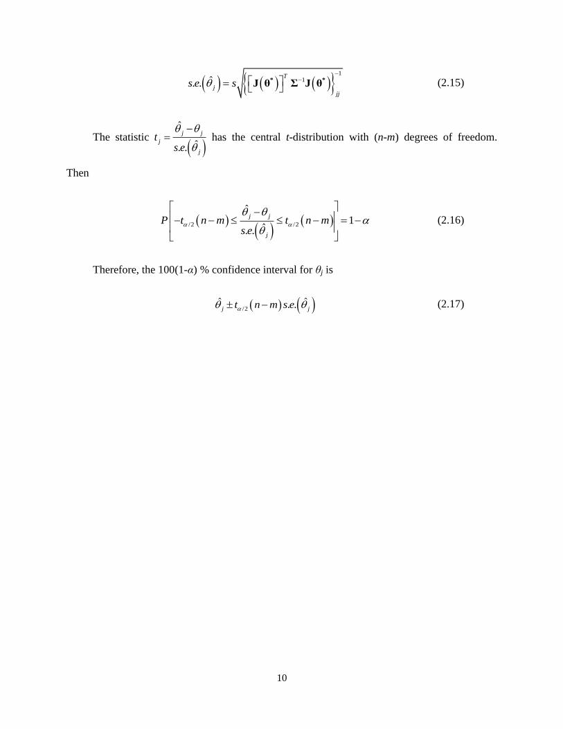
10

1

1ˆ. .T

jjj

s e s

* *J θ Σ J θ (2.15)

The statistic

ˆ

ˆ. .

j j

j

j

ts e

has the central t-distribution with (n-m) degrees of freedom.

Then

/2 /2

ˆ1

ˆ. .

j j

j

P t n m t n ms e

(2.16)

Therefore, the 100(1-α) % confidence interval for θj is

/2ˆ ˆ. .j jt n m s e (2.17)

11

Chapter 3 Uncertainty Analysis in Two Typical Analytical Model

Pumping tests are routinely used for the determination of hydraulic characteristics of

aquifer, especially the values of transmissivity and storage coefficient, through constant pumping,

and observing the aquifer's "response" (drawdown) in observation wells. Pumping tests are

typically interpreted by using an analytical model of aquifer flow (Thiem or Theis equations

without boundaries) to match the data observed in the field experiment.

In the real word, we cannot always get the exact value of pumping rate. Also, the aleatory

uncertainty in the observation is irreducible. In this chapter, I will study what happens in these

traditional analyses when the pumping rate and/or observations are uncertain, using Matlab

Regression Toolbox.

3.1 Steady-State Model (Thiem Equation)

Steady-state radial flow to a pumping well (Figure 3) is commonly called the Thiem

solution (Thiem 1906). It is commonly written as:

ln2

erQs r

T r

(3.1)

in which

s(r): drawdown at distance r

Q: discharge rate of the pumping well

T: transmissivity

re: radius of influence, or the distance at which the head is still h0

r: distance between the observation well and pumping well

http://en.wikipedia.org/wiki/Pump

http://en.wikipedia.org/wiki/Drawdown_(hydrology)

http://en.wikipedia.org/wiki/Water_well

http://en.wikipedia.org/wiki/Transmissivity

12

However, the Thiem model never truly occurs in nature. This solution is derived by

assuming:

pumping well is fully screened in the tested confined aquifer.

aquifer is homogeneous and isotropic

large areal extent (no boundaries)

a circular constant head boundary (e.g., a lake or river in full contact with the aquifer)

surrounding the pumping well at a distance re.

equilibrium has been reached

In this model, we usually calibrate the transmissivity T based on the real pumping data and

observed drawdown data.

3.1.1 Method 1

In this method, we are going to estimate one T to fit all the data sets. The steps are

described as follows:

1. Given true pumping rate Q0 = 2500 ft3/day, transmissivity T0 = 300 ft2/day, use the

Thiem Equation 0

0

0

ln2

eQ rs

T r

to generate true drawdown s0

2. There are N (N=5 in this method) observation wells and one pumping well. To

simplify the problem, we assume the distances from each observation well to the pumping well

are the same. The observed drawdown in each observation well should be the same theoretically.

So it can be considered that there is only one observation well but with N series of observations.

3. Assume the pumping rate Q and drawdown s are normal distributed with the mean

value of Q0 and s0, coefficient of variation δQ (=σQ/Q0) and δs (=σs/s0), respectively.

4. Now we have M (M = 1000 in this method) realizations:

1 11 12 1 2 21 22 2 1 2, , , , , , ,N N M M M MNQ s s s Q s s s Q s s s

5. Use Matlab Regression Toolbox to estimate T

Case A: fixed pumping rate, uncertain drawdown s

http://en.wikipedia.org/wiki/Lake

http://en.wikipedia.org/wiki/River

13

Using data sets 0 11 12 1 0 21 22 2 0 1 2, , , , , , ,N N M M MNQ s s s Q s s s Q s s s , calculate T

which minimizes the objective function:

2

0

1 1

ln2

M Ne

ij

i j

Q rT s

T r

(3.2)

The minimum value of Φ occurs when the gradient is zero:

0 0

21 1

12 ln ln 0

2 2

M Ne e

ij

i j

Q r Q rs

T T r r T

(3.3)

2

0 0

1 1 1 1

1ln ln

2 2

M N M Ne e

ij

i j i j

Q r Q rs

r T r

2

0

1 1 0 0

0

1 11 1

lnln ln2

2 2ln

2

M Ne

i j e e

M NM Nije

ijiji ji j

Q r

Q r r Q r rr MNT

sQ rss

r

(3.4)

0 0

0

0

ln ln

22

e e

ij

Q r r Q r rE T T

sE s (3.5)

Figure 4 shows the shows the regression results for the estimated T along with the 95%

confidence intervals for different levels of uncertainty in the drawdown observations (given by

the coefficient of variation). The estimated T is unbiased in this case. It is not related with the

number of calibration data used. As shown in Figure 4, we can find that the estimated T/T0 is

slightly fluctuating about the true value. The error is less than 2% which is negligible. This is an

aleatory error caused by the randomness in the drawdown observations. As to the 95%

confidence interval, it increases slightly with the increasing coefficient of variation of drawdown.

The confidence interval will be smaller if we have more data.

Case B: Uncertain pumping rate Q, fixed drawdown

14

Since the drawdown of each observation well is equal to s0, we use data sets

1 0 2 0 0, , , ,MQ s Q s Q s to calculate the T which minimizes the objective function:

2

0

1

ln2

Mi e

i

Q rT s

T r

(3.6)

In other words, we repeat this pumping experiment for M (M=1000) times and try to find

out one T which can minimize all the data sets.


0 21

12 ln ln 0

2 2

Mi e i e

i

Q r Q rs

T T r r T

(3.7)

Arrange this equation, we can get:

2

22

1 10

1 1 00

11

lnln21

ln ln2 2 2

ln2

M Mi e

iM Mi ei e i e i

MMi i i e

i

ii

Q rQ

r rrQ r Q rs T

Q rr T r sQs

r

(3.8)

22 2 2

0

0 0 0 0

2

0

2

0 0

2

0

ln ln ln

2 2 2

ln1

2

1

i ii Qe e e

i i

Qe

Q

E Q var QE Q Qr r r r r rE T

s E Q s E Q s Q

Q r r

s Q

T

(3.9)

The estimated T is biased depending on the mean and the variance of the pumping data.

The bias increases with increasing variance and decreases with increasing mean value. This is

demonstrated by the mathematical analysis above. In addition, the bias is not related to the

number of calibration data used. As to the 95% confidence interval, it also increases with the

coefficient of variation. This is obvious from equation(2.17). The Matlab Regression results are

coincident with the analytical solution (shown in Figure 5).

15

Case C: Uncertain pumping rate Q, uncertain drawdown s

Using data sets 1 11 12 1 2 21 22 2 1 2, , , , , , ,N N M M M MNQ s s s Q s s s Q s s s , calculate the T

which minimizes the objective function:

2

1 1

ln2

M Ni e

ij

i j

Q rT s

T r

(3.10)


2

1 1

12 ln ln 0

2 2

M Ni e i e

ij

i j

Q r Q rs

T T r r T

(3.11)

2

1 1 1 1

1ln ln

2 2

M N M Ni e i e

ij

i j i j

Q r Q rs

r T r

2

2

1 1

1 1

lnln2

2ln

2

M Ni e

i j ie

M Nij ii e

ij

i j

Q r

Qr rrT

s QQ rs

r

(3.12)

Assuming Q and s are independent,

22

2 2 2

0 0

2

0 0 0 0

2

0

ln ln

2 2

ln ln1

2 2

1

i iie e

ij i ij i

Q Qe e

Q

E Q var QE Qr r r rE T

E s Q E s E Q

Qr r Q r r

s Q s Q

T

(3.13)

In this regression, we assume the pumping and drawdown errors have the same coefficient

of variation (=standard deviation/mean). Figure 6 shows the very similar results as in Case B

(Figure 5). The uncertainty of drawdown doesn’t affect the T estimation. The bias of estimated T

is only depending on the mean and the variance of the pumping data. It is not related with the

16

number of calibration data used. This can be proved by the mathematical analysis above. The

confidence interval increases with the coefficient of variation. It is smaller than Case B, because

using more data can makes T more accurate.

3.1.2 Method 2

In method 1, we estimated one T using the whole data set, including the different

realizations for the pumping rate. However, in the real world, we usually estimate T for each

individual experiment. We may repeat the same experiment and average the estimated T to

reduce the error caused by the measurement. This is core thought of method 2. We generate the

realizations of data sets containing pumping rate and drawdown using the same steps as method

1 above (N =5, M = 1000).

Case A: fixed pumping rate, uncertain drawdown s

Using each data set 0 1 2, ,i i iNQ s s s to calculate the Ti which minimizes the objective

function:

2

0

1

ln2

Ne

ijij i

Q rT s

T r

(3.14)


0 0

21

12 ln ln 0

2 2

Ni e e

ij

j i

Q r Q rs

T T r r T

(3.15)

2

0 0

1 1

1ln ln

2 2

N Ne e

ij

j j i

Q r Q rs

r T r

2

0

1 0 0

0

1 11

lnln ln2 1

12 2ln

2

Ne

j e e

i N NNe

ij ijijj jj

Q r

Q r r Q r rr NT

Q rs ss

Nr

(3.16)

17

0

1 1

1

ln1 1 1

12

M Me

i Ni i

ij

j

Q r rT T

M Ms

N

(3.17)

Let’s consider an extreme case: N=1

0 0

0

1 1 1

ln1 1 1 1

2

M M Me

i

i i ii i

Q r r sT T T

M M s M s

(3.18)

Since0

1

11

M

i i

sE

M s

, from the equation (3.18) we can see that the expectation of

estimated T is biased in this extreme condition, which is opposite to the result of method 1. Most

important, this bias is related to the number of calibration data used. It is obvious that the bias

will gradually approach to 1 while the number of data increases (Figure 7). Besides, the variance

of T will also decrease significantly with the increasing number of data (Figure 8), although it

still increases slightly with the increasing coefficient of variation of drawdown error. These are

consistent with our common logic and sense that repeated trials can reduce the error and

uncertainty effectively.

Case B: Uncertain pumping rate Q, fixed drawdown

Since the drawdown of each observation well is equal to s0, we use each data set 0,iQ s

to calculate the Ti in the i’th experiment from the Thiem Equation directly:

0

ln2

i ei

Q rT

s r

(3.19)

1 0 0

1ln ln

2 2

Mi e i e

i

i

Q r Q rT T

M s r s r

(3.20)

00

0 0

ln ln2 2

ie e

E Q r Q rE T T

s r s r

(3.21)

18

2

0 0

ln ln

2 2

i e e

i i

Q r r r rVAR T VAR VAR Q

s s

(3.22)

Analytically, T is unbiased in this case, which is opposite to the result of method 1 (as

shown by comparing Figure 9 and Figure 5). It is not related with the number of calibration data

used. The variance of Ti is a constant times the variance of Qi (Figure 10), so it is larger than in

Case A. Because there is only one Qi in each experiment, actually the pumping rate is fixed in

each experiment, which doesn’t reflect the uncertainty. In addition, T and Q are linearly related

in the Thiem equation, so the expectation of estimated T is unbiased and its variance is

proportional to the variance of pumping rate, as proved by equation (3.21) and (3.22).


Using each data set (Qi, si1, si2…siN), (i =1…M, M = 1000, N = 5) to calculate the Ti which

minimizes the objective function:

2

1

ln2

Ni e

i ij

j

Q rs

T r

(3.23)


2

1

12 ln ln 0

2 2

Ni i e i e

ij

j

Q r Q rs

T T r r T

(3.24)

2

1 1

1ln ln

2 2

N Ni e i e

ij

j j

Q r Q rs

r T r

2

1

1 11

lnln ln2 1

12 2ln

2

Ni e

j i e i e

i N NNi e

ij ijijj jj

Q r

Q r r Q r rr NT

Q rs ss

Nr

(3.25)

This result is similar to that of Case A. Although Q is uncertain in this case, there is only

one fixed value of Q in each experiment. Thus, the Q uncertainty will not affect the estimation of

19

T. In Figure 11, we assume the pumping and drawdown errors have the same coefficient of

variation (=mean/variance). The estimated T has the similar statistical characteristics as shown in

Case A. As to the coefficient of variation of estimated T (Figure 12), the result is larger than that

in both Case A and Case B, which is caused by the variance of pumping rate and drawdown. But

the variance still decreases with increasing number of data. As long as the number of data is

enough, the estimated T can be considered as unbiased.

3.2 Transient Model (Theis Equation)

The Theis equation was created by C. V. Theis in 1935, for two-dimensional radial flow to

a point source in an infinite, homogeneous aquifer (Figure 13) (Theis 1935).

,

4

Qs r t W u

T (3.26)

in which

s(r,t): drawdown at distance r and time t

Q: discharge rate of the pumping well

T: transmissivity

W(u): well function, u

u

eW u du

u

u: dimensionless time parameter, 2

4

r Su

tT

r: distance between the observation well and pumping well

S: storativity

t: time

http://en.wikipedia.org/wiki/Transmissivity

20

The assumptions required by the Theis solution are similar to the Thiem equation. But it

doesn’t require constant head boundaries and equilibrium.

In this model, we usually calibrate the transmissivity T and storativity S based on the real

pumping data and the data of observed drawdown versus time.

3.2.1 Method 1

The steps are described as follows:

1. Set the number of time steps K for drawdown observations as 10. The initial time t(1)

as 0.0005 day, the initial time step Tstep as 0.01 day and the time step acceleration factor Tinc as

1.5. Then the observation time can be calculated by t(i+1) = t(i)+Tstep×Tinci.

2. Given true pumping rate Q0 = 2500 ft3/day, transmissivity T0 = 300 ft2/day, storage

S0 = 0.005, use the Theis Equation

2

0 00

0 04 4

Q r Ss W

T T t

to generate true drawdown s0(t).

3. There are N (N=5) observation wells and one pumping well. To simplify the problem,

we assume the distances from each observation well to the pumping well are the same. The

observed drawdown at a given time should be the same theoretically. So it can be considered that

there is only one observation well but with N series of observations.

4. Assume the pumping rate Q and drawdown s(t) are normally distributed with the

mean value of Q0 and s0(t), coefficient of variation δQ (=σQ/Q0) and δs(t) (=σs(t)/s0(t)), respectively.

5. We already have 10 data for each observation well, so we only need 100 realizations

in Theis Model to keep the total number of data the same as in Thiem Model. M (M = 100)

realizations at time t: (t=1…K, K=10):

1 11 12 1 2 21 22 2 1 2, , , , , , ,t t t t t t t t t

N N M M M MNQ s s s Q s s s Q s s s

Case A: Fixed pumping rate Q, uncertain drawdown s

Since the pumping rate is fixed, we use data sets 0 11 12 1, ,t t t

NQ s s s , 0 21 22 2, ,t t t

NQ s s s ,...,

0 1 2, ,t t t

M M MNQ s s s

21

1: Given storativity S0, estimate the transmissivity T which minimizes the objective

function:

22

0 0

1 1 1 4 4

M N Kt

ij

i j t

Q r ST s W

T Tt

(3.27)

The estimated T is shown in Figure 14 and is unbiased in this case. It is not related with the

number of calibration data used. This result is very similar to Figure 4. We can find that the

estimated T/T0 is slightly fluctuating about the true value. The error is less than 2% which is

negligible. This is an aleatory error caused by the randomness in the observed drawdown. As to

the confidence interval, it increases slightly with the increasing coefficient of variation of

drawdown. It will decrease with increasing number of observation data.

2: Given transmissivity T0, estimate the storativity S, which minimizes the objective

function:

22

0

1 1 1 0 04 4

M N Kt

ij

i j t

Q r SS s W

T T t

(3.28)

From the Figure 15 we can find that the estimated S is unbiased in this case. The estimated

S/S0 is slightly fluctuating about the true value. The error is less than 2% which is negligible.

This is an aleatory error caused by the randomness due to measurement error in drawdown. As to

the confidence interval, it increases slightly with the increasing coefficient of variation of

drawdown. The confidence interval should decrease if we have more realizations.

3: Estimate the transmissivity T and storativity S simultaneously, which minimize the

objective function:

22

0

1 1 1

,4 4

M N Kt

ij

i j t

Q r ST S s W

T Tt

(3.29)

The estimated T and S are unbiased in this case (Figure 16 and Figure 17). This is

consistent with the results of separated estimation. The estimated T and S are fluctuating about

22

the true value. Then confidence intervals of both T and S are larger than the result of separated

estimation. This is because when estimate T or S singly, the other parameter is given which

makes the estimation more accurate. The confidence interval of S is larger than that of T in this

case. Also, from the calculation by Matlab Regression toolbox, the covariance of T and S are

close to zero, which indicates they are independent.

Case B: Uncertain pumping rate Q, fixed drawdown s

Since the drawdown of each observation well is equal to s0, we use data sets 1 0, tQ s ,

2 0, tQ s ,..., 0, t

MQ s


function:

22

00

1 1 4 4

M Kt i

i t

Q r ST s W

T Tt

(3.30)

In Figure 18 we can find that the estimated T is biased depending on the mean and the

variance of the pumping data. The bias is linear with square of coefficient of variance which is

very similar to the result in Thiem Equation Method 1 Case B (Figure 5), but the confidence

interval is smaller using the same number of data. In addition, the bias is not related with the

number of calibration data used. As to the confidence interval, it also increases with the

coefficient of variation.


function:

22

0

1 1 0 04 4

M Kt i

i t

Q r SS s W

T T t

(3.31)

23

The result is shown in Figure 19. As the increasing of the coefficient of variation, the

estimated S increases dramatically. The bias of estimated S is huge compared with T. However,

the confidence interval is also large and it increases with increasing coefficient of variance.

3: Estimate the transmissivity T and storativity S simultaneously, to minimize the objective

function:

22

0

1 1

,4 4

M Kt i

i t

Q r ST S s W

T Tt

(3.32)

As shown in Figure 20 and Figure 21, the bias of estimated T and S will increase with the

increasing coefficient of variation of pumping rate. The bias of S is larger than that of T, but is

much smaller than the result in Figure 19. The covariance of T and S are close to zero which

indicates that they are independent.


In this regression, we assume the pumping and drawdown have the same coefficient of

variation, using data sets 1 11 12 1, ,t t t

NQ s s s , 2 21 22 2, ,t t t

NQ s s s ,…, 1 2, ,t t t

M M M MNQ s s s


function:

22

0

1 1 1 4 4

M N Kt iij

i j t

Q r ST s W

T Tt

(3.33)

As it shown in Figure 22, the result is exactly the same as in Case B (Figure 18). The

uncertainty of drawdown doesn’t affect the T estimation (proved in Case A, Figure 14). But it

does increase the confidence interval of T. The bias of estimated T is only depending on the

mean and the variance of the pumping data. The result is not related with the number of

calibration data used. The confidence interval increases with the increasing coefficient of

variation.

24


function:

22

1 1 1 0 04 4

M N Kt iij

i j t

Q r SS s W

T T t

(3.34)

Figure 23 shows the same results as in Case B. The uncertainty of drawdown doesn’t affect

the parameter estimation. But it does increase the confidence intervals of both T and S. The

confidence interval increases with the coefficient of variation. The estimated T and S are

fluctuating about the true value.


objective function:

22

1 1 1

,4 4

M N Kt iij

i j t

Q r ST S s W

T Tt

(3.35)

In this case, the T and S are biased (Figure 24 and Figure 25). This is consistent with the

results of separated estimation. These results are similar to the Case B. The bias increases with

the increasing coefficient of variation. The bias of estimated S is much larger than that of T.

Since the drawdown uncertainty doesn’t cause the bias of T and S, the uncertainty of pumping

rate dominates the impact of estimation.

3.2.2 Method 2

In this method, we will generate data the same as method 1. Then we will estimate T

and/or S for each pumping realization.

Case A: Fixed pumping rate Q, uncertain drawdown s

Since the pumping rate is fixed, we use data sets 0 1 2, ,t t t

i i iNQ s s s , for t = t1, t2…tK, K =10;

i = 1… M, M = 1000; N = 5

25

1: Given storativity S0, estimate the transmissivity Ti directly using Theis Equation:

22

0 0

1 1 4 4

N Kt

i ij

j t i i

Q r ST s W

T Tt

(3.36)

In this case, the estimated T is biased, which it opposite to the result in Method 1.

Although the objective function cannot be differentiated analytically, we can make an analogy

from the Thiem Equation. These results are similar to those in the same case of Thiem Equation

(Figure 7). Most important, this bias is related to the number of calibration data used. It is

obvious that the bias will gradually approach one while the number of data increases (Figure 26).

So we can consider it is unbiased as long as we have enough data. In addition, the coefficient of

variation of T will also decrease significantly with the increasing number of data (Figure 27).

These are consistent with our common logic and sense that repeated trials can reduce the error

and uncertainty effectively.

2: Given transmissivity T0, estimate the storativity Si directly using Theis Equation:

22

0

1 1 0 04 4

N Kt i

i ij

j t

Q r SS s W

T T t

(3.37)

With the analogy of the estimation of T, the estimated S should have the same

characteristics (as shown in Figure 28 and Figure 29). We don’t repeat it here.


objective function:

22

0

1 1

,4 4

N Kt i

i i ij

j t i i

Q r ST S s W

T Tt

(3.38)

The result is similar to the result of the same case in method 1. The estimated T and S are

unbiased as long as we have enough data in this case. The estimated T and S are fluctuating

about the true value (Figure 30 and Figure 32). But the coefficient of variation of T and S are

greater than the result in the separated estimation (Figure 31 and Figure 33). Also, the covariance

26

of T and S, calculated by the Matlab Regression Toolbox, are close to zero, which indicates they

are independent.

Case B: Uncertain pumping rate Q, fixed drawdown s

Since the drawdown of each observation well is equal to s0, we use each data set 0, t

iQ s ,

for t = t1, t2…tK, K =10; i = 1… M, M = 100

1: Given storativity S0, estimate the transmissivity Ti directly using the Theis Equation:

2

00

4 4

t i

i i

Q r Ss W

T Tt

(3.39)

This is an implicit equation which cannot be solved analytically. But the result could be

written in the form of:

i iT g Q (3.40)

Since g(Qi) is a nonlinear equation, i iE T g E Q

1

M

i i i

i

E T g Q P Q Q

(3.41)

So there should be some bias of T in this case.

Although there is not an apparent bias in Figure 34, the bias does exist according to the

above analysis. The bias is less than 1% which is negligible. Compared with the results in Thiem

Model Method 2 Case B (Figure 9), which is unbiased because of the linearity, this bias is

caused by the non-linearity. The coefficient of variation of estimated T (Figure 35) is

proportional to the coefficient of variation of pumping rate approximately and it is close to the

result in Thiem Model Method 2 Case B (Figure 10).

2: Given transmissivity T0, estimate the storativity Si directly using Theis Equation:

27

2

0

0 04 4

t iQ r Ss W

T T t

(3.42)

By analogy with the estimation of T, the estimated S should have the same characteristics

(as shown in Figure 36 and Figure 37 ). The bias of S is still large which is similar to that of Case

B in Method 1 of Theis Equation (Figure 19). The coefficient of variation of S is similar to that

of similar to that of T.


objective function:

22

0

1

,4 4

Kt i i

i i

t i i

Q r ST S s W

T Tt

(3.43)

In this case, since there is only one fixed Qi in each experiment, this regression problem

degenerates into an equations solving problem. For a particular Qi, we can write it in the form of

Qi=b×Q0, in which b is fluctuating about 1. Then we can solve the equations:

2

00

4 4

t i

i i

bQ r Ss W

T Tt

We can just keep the i

i

S

T as a constant in the well function, and set Ti = bT0. Obviously, the

solution will be

0

0

0

0

ii

ii

QT T

Q

QS S

Q

, which is unbiased as shown in Figure 38 and Figure 40.

These results are opposite to the results of separate estimation. The coefficient of variation

of estimated T (Figure 39) is close to the result in separate estimation (Figure 35). However, the

coefficient of variation of estimated S (Figure 41) becomes very small in this case.


28

Using data sets 1 2, ,t t t

i i i iNQ s s s , for t = t1, t2…tK, K =10; i = 1… M, M = 1000; N = 5

1: Given storativity S0, estimate the transmissivity Ti which minimizes the objective

function:

22

0

1 1 4 4

N Kt i

i ij

j t i i

Q r ST s W

T Tt

(3.44)

In this case, the estimated T is biased (Figure 42). These results combine both the impact of

uncertain pumping and uncertain drawdown as shown in Case A and Case B. Increasing the

number of data will reduce the bias and coefficient of variation of T (Figure 43). However, this

impact is not as significant as that in Case A, because the pumping rate uncertainty dominates

the impact.

2: Given transmissivity T0, estimate the storativity Si which minimizes the objective

function:

22

1 1 0 04 4

N Kt i i

i ij

j t

Q r SS s W

T T t

(3.45)

Compared with the bias caused by uncertain drawdown in Case A (Figure 28) and

uncertain pumping in Case B (Figure 36), the impact of uncertain drawdown is small. As a result,

the impact of the number of data is not apparent in Figure 44 and Figure 45. These indicate the

domination of uncertain pumping again. In all, by analogy with the estimation of T, the estimated

S has the same characteristics.


objective function:

22

1 1

,4 4

N Kt i i

i i ij

j t i i

Q r ST S s W

T Tt

(3.46)

29

In this case, the T and S are biased which is consistent with the result of separated

estimation. The increasing number of data will reduce the bias and the coefficient of variation (as

shown in Figure 46, Figure 47, Figure 48 and Figure 49).

3.3 Comparison and Conclusion

The uncertainty analysis of Thiem and Theis model are summarized in the Table 1. The

bias and variance shown in the table are the values at square of coefficient of variation equal to

0.5. Although the results change for different levels of uncertainty in s and Q, the value in Table

1 can show the characteristics of uncertainty.

In method 1, the parameters are unbiased when only drawdown is uncertain in both Thiem

and Theis models. The uncertainty of pumping rate dominates the impact on parameter

estimation. So the biases of estimated parameters are close when pumping rate is uncertain. Also,

in the Theis model, the bias of estimated S is relatively large, compared with T.

In method 2, bias is commonly existed. For the uncertain Q in Thiem model, T is unbiased

because there is only one Q in each experiment which cannot reflect its uncertainty. For the

simultaneously estimation of T and S in Theis model, the results are all unbiased, although they

are biased when estimated separately. This might be caused by the dimensionless parameter

2

4

r S

Tt

in the well function. In the case of uncertain drawdown, the increasing number of observation

data will decrease the bias and variance of estimated parameters significantly. However, these

effects will not be apparent when Q is also uncertain. Same as in the method 1, the bias caused

by the uncertainty of pumping rate is dominant. In addition, the bias of estimated S is also very

large, same as method 1.

30

Chapter 4 Uncertainty Analysis of Partially Penetrating Stream

System Using PEST

4.1 Introduction

Stream-aquifer interactions are an important component of the hydrologic budgets of many

watersheds and have great significant socioeconomic and political ramifications (Bouwer 1997).

Over the last 60 years, several analytical models have been developed to assess the mechanism

of stream-aquifer system. Theis (1941) was the first to present a transient model to describe the

pumping activities under the stream impact. After Theis’s work, Glover and Balmer (1954)

modified it and published a method for determining river depletion based on a series of idealistic

assumptions that include fully penetrating river and full communication between river and

aquifer. Hantush (1965) extended this model to the system with imperfect hydraulic connections

between the aquifer and the stream. However, these methods are based on too many

assumptions and cannot meet the real conditions in many natural systems. Later on, Grigoryev

and Bochever developed a steady-state model of stream-aquifer interactions incorporating a

simplified representation of a partially penetrating stream. In 1999, Zlotnik gave a transient

solution for the Grigoryev–Bochever model (Zlotnik, Huang and Butler 1999).

In this chapter, the Zlotnik’s model (ZHB Model) is used to estimate the aquifer parameter

based on the observation of drawdown and river depletion.

4.2 Mathematical Description

The model is established to calculate the drawdown (as a function of x, y and t) and stream

depletion (as a function of t) produced by pumping from a fully penetrating well.

Consider hydraulic head h(x,y,t) in an aquifer with the aquifer base as a reference level,

and a stream stage H(t) with the same reference level. This two-dimensional groundwater flow

(Figure 50) can be described as:

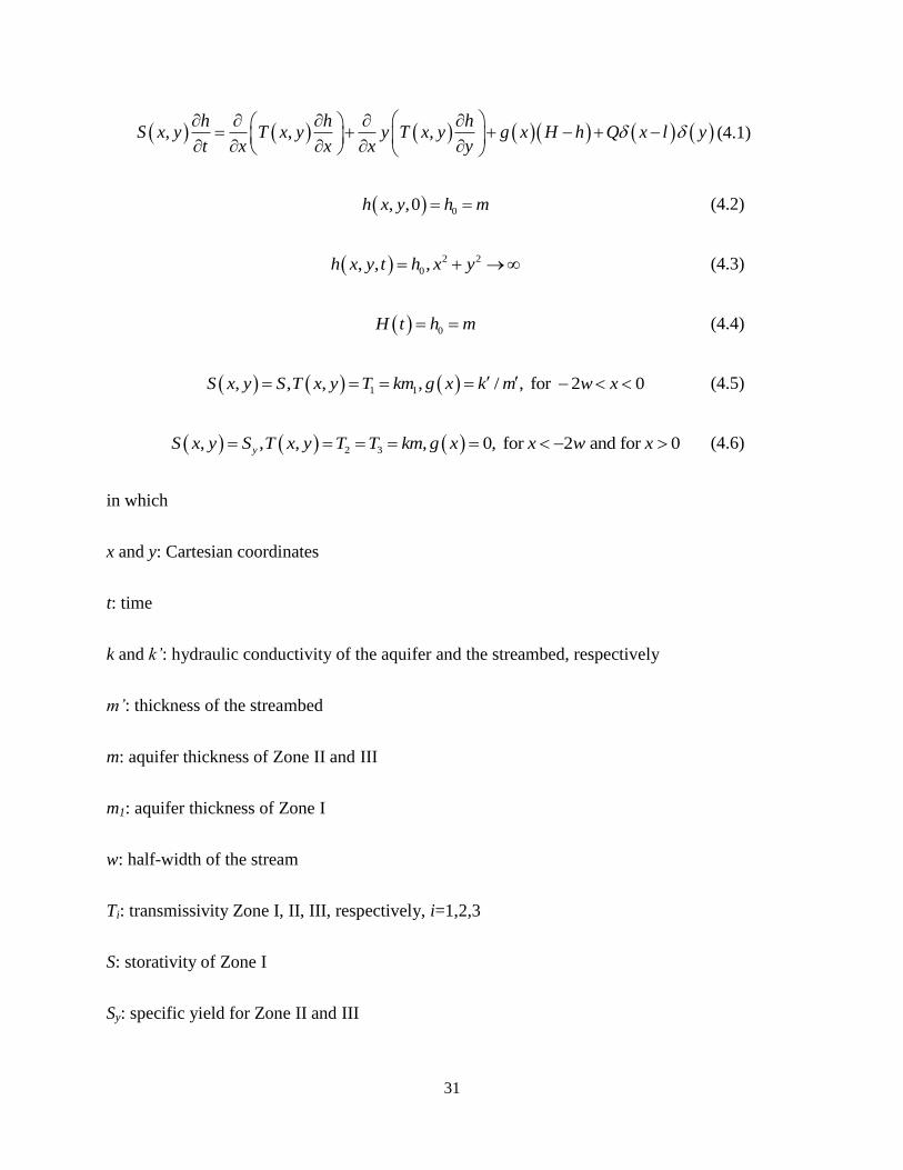
31

, , ,h h h

S x y T x y y T x y g x H h Q x l yt x x x y

(4.1)

0, ,0h x y h m (4.2)

2 2

0, , ,h x y t h x y (4.3)

0H t h m (4.4)

1 1, , , , / , for 2 0S x y S T x y T km g x k m w x (4.5)

2 3, , , , 0, for 2 and for 0yS x y S T x y T T km g x x w x (4.6)

in which

x and y: Cartesian coordinates

t: time

k and k’: hydraulic conductivity of the aquifer and the streambed, respectively

m’: thickness of the streambed

m: aquifer thickness of Zone II and III

m1: aquifer thickness of Zone I

w: half-width of the stream

Ti: transmissivity Zone I, II, III, respectively, i=1,2,3

S: storativity of Zone I

Sy: specific yield for Zone II and III

32

l: the distance from the well to the stream bank

Q: pumping rate

δ(x): the Dirac function

The riverbed leakage is integrated along the entire river bed, which can be expressed as

0

0

2

/sd

w

q t dy k h h m dx

(4.7)

The mathematical model defined by equations (4.1) through (4.6) was solved analytically

using an approach analogous to that of Butler and Liu (Butler and Tsou 2001). The solution is

obtained using integral transforms. A Laplace transform in time followed by a Fourier

exponential transform in length produces Fourier-Laplace space analogues to this model. Stream

depletion was calculated using the approach of Hunt(1991) with the transform-space using

analog of equation (4.7). The details are not provided here (Butler and Tsou 2001) .

4.3 Parameter Estimation Using PEST

For the inverse problem, we use both drawdown and depletion as observations to calibrate

transmissivity and specific yield in Zone II, and river bed conductivity. The steps are described

as follows:

1. Set the number of time steps K for drawdown observations as 10. The initial time t(1)

as 0.0005 day, the initial time step Tstep as 0.01 day and the time step acceleration factor Tinc as

1.5. Then the observation time can be calculated by t(i+1) = t(i)+Tstep×Tinci.

2. Given the true pumping rate Q0 = 1000, T0 = 200 and Sy0 = 0.2 in Zone II, k0 = 0.2 to

calculate the true drawdown s0(t) and stream depletion q0(t).

3. Assume the pumping rate Q, drawdown s(t) and depletion q(t) are normally

distributed with the mean value of Q0, s0(t) and q0(t), variance σQ, σs(t) and σq(t) respectively.

4. We already have 10 data for each observation well, so we only need 100 realizations

in this model to keep the total number of data the same as in Thiem and Theis Model. M (M =

100) realizations at time t: (t=1…K, K=10):

33

1 1 1 2 2 2, , , , , , ,t t t t t t

M M MQ s q Q s q Q s q

In this problem, we only use Method 2 described as in Thiem and Theis Model. PEST can

only estimate parameters for one model each time. In ZHB Model, we have one series

observation of drawdown and/or stream depletion. In other words, we can only use one data set

to estimate one parameter set, which is the thought in Method 2. The we repeat the estimation for

each of the M realizations of the data sets (reflecting uncertainty in drawdown, stream depletion

and pumping) as in Chapter 3.

Case A: Only use drawdown as the observation of regression

The objective function should be written as:

2

1 1

,M K

i

i t

s t f

θ x θ (4.8)

where θ is the estimated parameter, x is the all parameters except θ in this model, f is an implicit

function which calculates the drawdown.

In this case, we assume that there is the same degree of error in both drawdown s and

pumping rate Q. The separate estimation results are shown through Figure 51 through Figure 56.

All three parameters are biased. When pumping rate is fixed, the bias is relatively small. The

biases of T and Sy are relatively small, while the bias of k is larger. Also the coefficient of

variation of k is tremendous. This indicates the estimated k is not as reliable as estimated T or Sy.

By contrast, the result of T and Sy are more reasonable. They are similar to the results in both

Thiem and Theis Model. This is because when T and Sy are fixed, the sensitivity of river bed

conductivity to the respect of drawdown is small. The drawdown is dominated by T and Sy.

The simultaneously estimated parameters are shown through Figure 57 to Figure 62. The

covariance of estimated parameters calculated in PEST shows that they are uncorrelated. The

results of Sy are close to the separately estimated results. The biases Sy are greater while the bias

of k is smaller than the previous results. But the T is approximately unbiased in this case. The

coefficients of variation of T and Sy are much smaller in this estimation. Also, the coefficient of

34

variation of k is smaller than before though it is still large. This is because the drawdown is

considered as a consequence of all three parameters together. There is an issue of equifinality in

data assimilation (Beven 2006) that different sets of parameter values may fit the model equally

well without the ability to distinguish which set of parameter value is better than others.

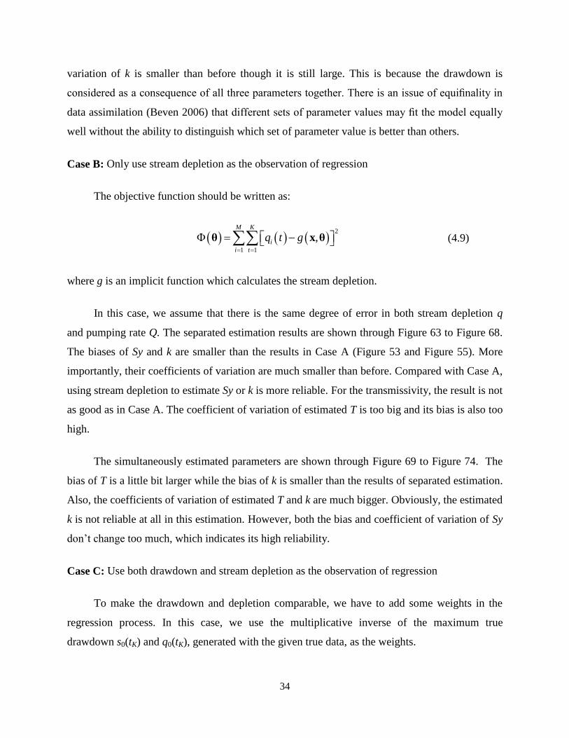
Case B: Only use stream depletion as the observation of regression


2

1 1

,M K

i

i t

q t g

θ x θ (4.9)

where g is an implicit function which calculates the stream depletion.

In this case, we assume that there is the same degree of error in both stream depletion q

and pumping rate Q. The separated estimation results are shown through Figure 63 to Figure 68.

The biases of Sy and k are smaller than the results in Case A (Figure 53 and Figure 55). More

importantly, their coefficients of variation are much smaller than before. Compared with Case A,

using stream depletion to estimate Sy or k is more reliable. For the transmissivity, the result is not

as good as in Case A. The coefficient of variation of estimated T is too big and its bias is also too

high.


bias of T is a little bit larger while the bias of k is smaller than the results of separated estimation.

Also, the coefficients of variation of estimated T and k are much bigger. Obviously, the estimated

k is not reliable at all in this estimation. However, both the bias and coefficient of variation of Sy

don’t change too much, which indicates its high reliability.

Case C: Use both drawdown and stream depletion as the observation of regression

To make the drawdown and depletion comparable, we have to add some weights in the

regression process. In this case, we use the multiplicative inverse of the maximum true

drawdown s0(tK) and q0(tK), generated with the given true data, as the weights.

35


2 2

1 1 max max

1 1, ,

M K

i i

i t

q t g s t fq s

θ x θ x θ (4.10)

In this case, we assume that there is the same degree of error in drawdown s, stream

depletion q and pumping rate Q. The separate estimation results are shown through Figure 75 to

Figure 80. The estimated k is more reliable with small bias and coefficient of variation. The

result of Sy is similar as before. In this case, the estimated T is unacceptable when pumping rate

is uncertain.


result of T is a little bit better than before but it’s still not reliable. The Sy and k doesn’t change

too much compared with Case A and Case B.

4.4 Comparison and Conclusion

The uncertainty analysis of ZHB model is summarized in the Table 2 through Table 4. The

bias and variance shown in the table are the approximated values at square of coefficient of

variation equal to 0.5. Although the results change for different levels of uncertainty in

observations and Q, the value in those tables can show the characteristics of uncertainty.

When we only use drawdown to estimate the parameters, the estimated k is unacceptable.

The coefficient of variation of k is too big which indicates its low reliability. This is caused by

the low sensitivity of k to drawdown observations. As for T, the result of separate estimation is

worse than that of simultaneously estimation. The results of Sy are all reliable, but the

simultaneously estimated Sy is better than separate estimated result. This might be caused by the

issue of equifinality.

When we only use stream depletion to estimate the parameters, the estimated Sy and k are

better than the first case. This is caused by their high sensitivity to observations of depletion. But

the result for T shows low reliability. By comparison, T is more sensitive to the drawdown and k

is more sensitive to the stream depletion.

36

When we use both drawdown and depletion to estimate the parameters, the results are not

improved very much. The T is even worse than Case A. But the Sy is similar as in Case A and

Case B, which shows high reliability. In this case, there are twice as much data as before, so the

results show less coefficient of variation.

37

Chapter 5 Pumping Data Analysis in the Republican River

Compact Administration (RRCA) Groundwater Model

5.1 Introduction

As stated by Vincent L. Mckusick: “The Republican River rises in the high plains of

northeastern Colorado and western Kansas and Nebraska. The river flows in a generally eastern

direction and encompasses approximately 24,900 square miles within its watershed that is

illustrated below (Figure 87). The States of Colorado, Kansas, and Nebraska, with the consent of

the United States of America, entered into the Republican River Compact in 1942 in order to

equitably divide the waters of the Republican River Basin. Ground water accretions and

depletions are subject to administration within the Compact for the portion of the basin that

contributes flow above the stream flow gaging station on the Republican River near Hardy,

Nebraska which is in the eastern part of the Republican River Basin near the Kansas Nebraska

state line. The primary purpose of the RRCA Model is to determine the amount, location, and

timing of stream flow depletions to the Republican River caused by well pumping and to

determine stream flow accretions from recharge of water imported from the Platte River Basin

into the Republican River Basin above the stream flow gaging station near Hardy, Nebraska.”

(Mckusick 2003)

Ground water pumping for irrigation in the Republican River Basin was limited prior to

World War II but progressed rapidly in the 1960’s and 1970’s. Figure 88 shows the cumulative

number of irrigation wells within the Republican River model domain over time. The States

agreed to accept the method each one developed to estimate gross irrigation pumping within their

respective boundaries for the period 1940-2000. The method used by each state for estimating

historical ground water pumping and tabulations of the annual pumping estimates are different,

which may cause pumping uncertainty.

The pumping for municipal and industrial purposes for Colorado and Nebraska was

obtained from the USGS and subsequently verified and refined by each state. Kansas developed

its estimates from its water use database. The program mkgw, developed by the RRCA,

distributes pumping from the county to the model cells by assigning pumping proportional to the

38

appropriated acreage of the active wells for that year. In other words, the entire pumping in the

county is computed and then divided by the county acreage to get pumping per acre. Then the

pumping in each Modflow cell is assigned according to irrigated acreage.

The RRCA Model applies a modified version of the United States Geological Survey

modular ground water model Modflow 2000 version 1.10 to numerically calculate stream

depletions from ground water pumping and accretions from imported water supplies.

The RRCA Model is spatially discretized into one-square mile grid cells and temporally

discretized into one-month stress periods, with two time-steps per stress period. Then the model

was calibrated to achieve an acceptable level of correspondence between model inputs, results

and historical physical observations of the ground water flow system in the Republican River

Basin.

5.2 Data Analysis

From the analysis in Chapter 3 and Chapter 4, we found that the uncertainty of pumping

data has significant impact on the parameter estimation. In this chapter, we are going to analyze

the pumping data and quantify its uncertainty in three counties of Nebraska: Perkins, Chase and

Dundy.

The Nebraska raw data consists of seven databases which can be downloaded from the

RRCA website:

the lands served exclusively by ground water irrigation database,

the commingled lands ground water irrigated database,

the lands served exclusively by surface water irrigation database,

the commingled surface water database,

the river pumpers database,

the private canals database,

the canal leakage database.

39

Each of the first four databases specifies the annual volume of applied water and area over

which it is applied on a cell-by-cell basis. The river pumpers database and private canals

database supply only the annual volume by cell and the canal leakage database supplies the

monthly volume by cell. The program “mknedat” is used to create the required monthly ground

water pumping files by distributing the annual cell-by-cell pumping to a monthly time step using

a fixed set of factors.

Figure 89 to Figure 91 show the annual pumping volume (acre-feet) for each county from

1980 to 2006. There are three kinds of data sets in each figure. The ‘.real’ file is the data set that

is recorded by the farmer or government. It is the real metered data from the field in the Upper

Republican Natural Resources District. We obtained a preliminary version of this data set for the

Upper Republican Natural Resources District from Professor Nicholas Brozovic, Department of

Agricultural and Consumer Economics, University of Illinois at Urbana-Champaign. The ‘.pmp’

file is the data set that combines all the pumping data for different usages, such as irrigation and

industry. The ‘.wel’ file is the data generated from the ‘.pmp’ data. It is used as the input file of

the RRCA Modflow Model. Both of ‘.pmp’ and ‘.wel’ data can be downloaded from the RRCA

website directly. For the total annual pumping volume, the ‘.pmp’ and ‘.wel’ data sets are very

close to each other in all three counties. For Perkins County, the real metered data are greater

than both the ‘.pmp’ and ‘.wel’ data. But they are very close during 1991~1996. For Chase

County, these three data sets are all close to each other. For Dundy County, the real metered data

are at least 20% greater than the ‘.pmp’ and ‘.wel’ data. There is an apparent bias of pumping

data is in this county. But for the year 2003, 2004 and 2005, these three data are very close

(Table 5).

Figure 92 to Figure 98 show the difference (in acre-feet) between the real pumping data

and Modflow data for each cell from 1980 to 2006. It is obvious that the pumping uncertainty is

non-negligible. The real pumping data is larger than the Modflow data, which corresponds to a

negative difference of the mean value, illustrated in these figures and Table 6. The difference is

approximately normally distributed based on visual impression.

40

Chapter 6 Conclusions and Future Work

6.1 Conclusions

In this thesis, we analyzed the impact of uncertain pumping and observations on the

parameter estimation using statistical methods in three typical simplified groundwater models.

The uncertainty analysis using the Matlab Regression Toolbox of the Thiem and Theis

models shows the significant impact of uncertain pumping. In method 1, the parameters are

unbiased when the pumping rate is fixed in both the Thiem and Theis models. The uncertainty of

the pumping rate dominates the impact on parameter estimation. The transmissivity is more than

50% overestimated when the coefficient of variation of pumping rate is 0.5. By comparison, the

impact of uncertain drawdown is negligible. In method 2, the bias of transmissivity is much

smaller than in method 1. Because there is only one Q in each experiment, it can be assumed that

the pumping rate is fixed in each experiment, which does not reflect the uncertainty. In addition,

the impact of drawdown can be reduced by increasing the number of observation data in this

method. For the simultaneous estimation of T and S in Theis model, the results are all unbiased,

although they are biased when estimated separately. This might be caused by the dimensionless

parameter

2

4

r S

Tt in the well function.

The uncertainty analysis using PEST for a more complex model with a partially

penetrating stream shows the impact of uncertain pumping, drawdown and stream depletion.

When we only use drawdown as the objective of regression (Case A), the bias of transmissivity

is similar to the results in the Thiem and Theis models. The impact of uncertain pumping is more

apparent compared with the impact of uncertain drawdown. It is unbiased in the simultaneous

estimation of T, Sy and k. However, the results of riverbed conductivity k are meaningless

because the coefficient of variation of estimated k is tremendous. This is caused by its low

sensitivity with respect to drawdown. When we only use stream depletion as the objective of

regression (Case B), the bias of T is similar as before while its coefficient of variation is too big

to make it reliable. This is because the transmissivity is not sensitive with respect to stream

depletion. By contrast, the estimated k is more acceptable than in Case A. In Case C, we use both

41

drawdown and stream depletion as the objective of regression. The results of T and k are less

credible than before. In these three cases, the estimated Sy is always good with a lower bias and a

smaller coefficient of variation. The result for T shows low reliability.

In the section of data analysis, we estimated the pumping uncertainty in a real case by

studying the data from the RRCA model from 1980 to 2006. In this unusual case, we have actual

metered pumping data, as well as an assumed pumping rate that was used in the RRCA model.

We compared the annual pumping volume for each county between the ‘real’, ‘pmp’ and ‘wel’

data. The ‘.pmp’ and ‘.wel’ data sets are very close for all three counties. For Perkins County, the

real metered data are greater than both the ‘.pmp’ and ‘.wel’ data. But they are very close during

1991~1996. For Chase County, these three data sets are all close to each other with small

fluctuation. For Dundy County, the real metered data are at least 20% greater than the ‘.pmp’ and

‘.wel’ data. There is an apparent bias of pumping data is in this county. But for 2003, 2004 and

2005, these three data sets are almost the same. Furthermore, we compared the real pumping data

and Modflow data for each cell in all three counties. It is obvious that the pumping uncertainty is

non-negligible. The real pumping data is larger than the Modflow data for the Upper Natural

Resources District of Nebraska, which is shown as a negative mean value of difference in these

figures. The difference is approximately normally distributed. This result is consistent with the

assumption when we randomly generated the uncertain pumping in the uncertainty analysis.

6.2 Future Work

This research will provide advances in the development and calibration of groundwater

models and also provide practical information on how to deal with uncertain input data. However,

there are still some issues far from being solved. The models used in this thesis are based on

assumptions that never or hardly occur in nature. We need to do the regression using more

realistic models such as a Modflow numerical model. In addition, the number of estimated

parameters is only two or three based on the assumption of homogeneity in this thesis. In the real

field, the transmissivity and storativity are spatially related. In this case, the number of estimated

parameters might be greater than the number of observations. The impact of uncertain input may

lead to some other issues.

42

The uncertainty and bias of the pumping rate is obvious in the RRCA model. This is a

complicated numerical Modflow model with a large amount of aquifer parameters. We need to

apply the impact of uncertainty to the RRCA model. Also we need to explore the impact of the

bias of the pumping rate.

43

Chapter 7 Figures and Tables

Figure 1 Uncertainty in annual ground-water pumpage estimates developed for Death Valley regional ground-water flow

system model domain, 1913–98 (Moreo, et al. 2003)

Figure 2 Iterative improvement of initial parameter values toward the global objective function minimum (Lin 2005)

44

Figure 3 Confined Aquifer System and Thiem Schema

Figure 4 Estimation of T with Fixed Q and Uncertain s (Thiem-Method 1-Case A)

45

Figure 5 Estimation of T with Uncertain Q and Fixed s (Thiem-Method 1-Case B)

Figure 6 Estimation of T with Uncertain Q and Uncertain s (Thiem-Method 1-Case C)

46

Figure 7 Estimation of T with Fixed Q and Uncertain s (Thiem-Method 2-Case A)

Figure 8 C.O.V. of Estimated T with Fixed Q and Uncertain s (Thiem-Method 2-Case A)

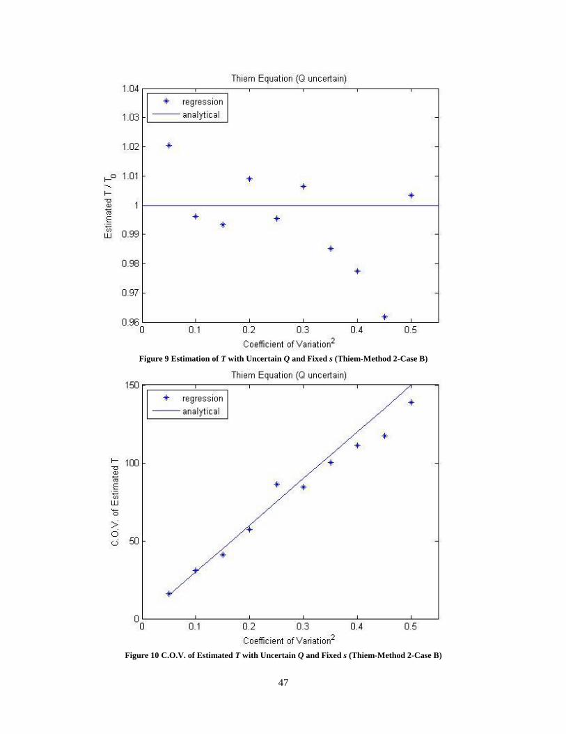
47

Figure 9 Estimation of T with Uncertain Q and Fixed s (Thiem-Method 2-Case B)

Figure 10 C.O.V. of Estimated T with Uncertain Q and Fixed s (Thiem-Method 2-Case B)

48

Figure 11 Estimation of T with Uncertain Q and Uncertain s (Thiem-Method 2-Case C)

Figure 12 C.O.V. of Estimated T with Uncertain Q and Uncertain s (Thiem-Method 2-Case C)

49

Figure 13 Confined Aquifer System and Theis Schema

Figure 14 Estimation of T with Fixed Q and Uncertain s (Theis-Method 1-Case A)

50

Figure 15 Estimation of S with Fixed Q and Uncertain s (Theis-Method 1-Case A)

Figure 16 Simultaneously Estimation of T with Fixed Q and Uncertain s (Theis-Method 1- Case A)

51

Figure 17 Simultaneously Estimation of S with Fixed Q and Uncertain s (Theis-Method 1- Case A)

Figure 18 Estimation of T with Uncertain Q and Fixed s (Theis-Method 1-Case B)

52

Figure 19 Estimation of S with Uncertain Q and Fixed s (Theis-Method 1-Case B)

Figure 20 Simultaneously Estimation of T with Fixed Q and Uncertain s (Theis-Method 1- Case B)

53

Figure 21 Simultaneously Estimation of S with Fixed Q and Uncertain s (Theis-Method 1- Case B)

Figure 22 Estimation of T with Uncertain Q and Uncertain s (Theis-Method 1-Case C)

54

Figure 23 Estimation of S with Uncertain Q and Uncertain s (Theis-Method 1-Case C)

Figure 24 Simultaneously Estimation of T with Uncertain Q and Uncertain s (Theis-Method 1- Case C)

55

Figure 25 Simultaneously Estimation of S with Uncertain Q and Uncertain s (Theis-Method 1- Case C)

Figure 26 Estimation of T with Fixed Q and Uncertain s (Theis-Method 2-Case A)

56

Figure 27 C.O.V. of Estimated T with Fixed Q and Uncertain s (Theis-Method 2-Case A)

Figure 28 Estimation of S with Fixed Q and Uncertain s (Theis-Method 2-Case A)

57

Figure 29 C.O.V. of Estimated S with Fixed Q and Uncertain s (Theis-Method 2-Case A)

Figure 30 Estimated T for Simultaneous Estimation of T and S with Fixed Q and Uncertain s (Theis-Method 2- Case A)

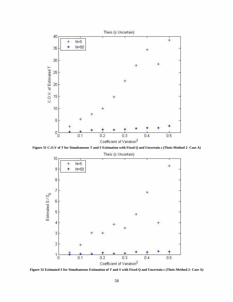
58

Figure 31 C.O.V of T for Simultaneous T and S Estimation with Fixed Q and Uncertain s (Theis-Method 2- Case A)

Figure 32 Estimated S for Simultaneous Estimation of T and S with Fixed Q and Uncertain s (Theis-Method 2- Case A)

59

Figure 33 C.O.V of S for Simultaneous T and S Estimation with Fixed Q and Uncertain s (Theis-Method 2- Case A)

Figure 34 Estimation of T with Uncertain Q and Fixed s (Theis-Method 2-Case B)

60

Figure 35 C.O.V. of Estimated T with Uncertain Q and Fixed s (Theis-Method2-Case B)

Figure 36 Estimation of S with Uncertain Q and Fixed s (Theis-Method2-Case B)

61

Figure 37 C.O.V. of Estimated S with Uncertain Q and Fixed s (Theis-Method2-Case B)

Figure 38 Estimated T for Simultaneous Estimation of T and S with Uncertain Q and Fixed s (Theis-Method 2- Case B)

62

Figure 39 C.O.V. of T for Simultaneous T and S Estimation with Uncertain Q and Fixed s (Theis-Method 2- Case B)

Figure 40 Estimated S for Simultaneous Estimation of T and S with Uncertain Q and Fixed s (Theis-Method 2- Case B)

63

Figure 41 C.O.V of S for Simultaneous T and S Estimation with Uncertain Q and Fixed s (Theis-Method 2- Case B)

Figure 42 Estimation of T with Uncertain Q and Uncertain s (Theis-Method2-Case C)

64

Figure 43 C.O.V. of Estimated T with Uncertain Q and Uncertain s (Theis-Method2-Case C)

Figure 44 Estimation of S with Uncertain Q and Uncertain s (Theis-Method2-Case C)

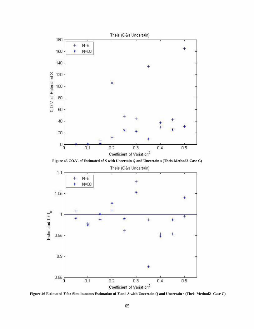
65

Figure 45 CO.V. of Estimated of S with Uncertain Q and Uncertain s (Theis-Method2-Case C)

Figure 46 Estimated T for Simultaneous Estimation of T and S with Uncertain Q and Uncertain s (Theis-Method2- Case C)

66

Figure 47 C.O.V of T for Simultaneous T and S Estimation with Uncertain Q and Uncertain s (Theis-Method 2- Case C)

Figure 48 Estimated S for Simultaneous Estimation of T and S with Uncertain Q and Uncertain s (Theis-Method2- Case C)

67

Figure 49 C.O.V of S for Simultaneous T and S Estimation with Uncertain Q and Uncertain s (Theis-Method 2- Case C)

Figure 50 Scheme of Grigoryey-Bochever Model (Zlotnik, Huang and Butler 1999)

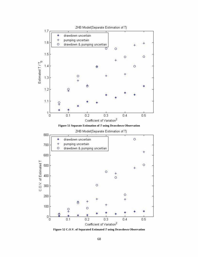
68

Figure 51 Separate Estimation of T using Drawdown Observation

Figure 52 C.O.V. of Separated Estimated T using Drawdown Observation

69

Figure 53 Separated Estimation of Sy using Drawdown Observation

Figure 54 C.O.V. of Separate Estimated Sy using Drawdown Observation

70

Figure 55 Separate Estimation of k using Drawdown Observation

Figure 56 C.O.V. of Separate Estimated k using Drawdown Observation

71

Figure 57 Simultaneously Estimation of T using Drawdown Observation

Figure 58 C.O.V. of Simultaneously Estimated T using Drawdown Observation

72

Figure 59 Simultaneously Estimation of Sy using Drawdown Observation

Figure 60 C.O.V. of Simultaneously Estimated Sy using Drawdown Observation

73

Figure 61 Simultaneously Estimation of k using Drawdown Observation

Figure 62 C.O.V. of Simultaneously Estimated k using Drawdown Observation

74

Figure 63 Separate Estimation of T using Depletion Observation

Figure 64 C.O.V. of Separate Estimated T using Depletion Observation

75

Figure 65 Separate Estimation of Sy using Depletion Observation

Figure 66 C.O.V. of Separate Estimated Sy using Depletion Observation

76

Figure 67 Separate Estimation of k using Depletion Observation

Figure 68 C.O.V. of Separate Estimated k using Depletion Observation

77

Figure 69 Simultaneously Estimation of T using Depletion Observation

Figure 70 C.O.V. of Simultaneously Estimated T using Depletion Observation

78

Figure 71 Simultaneously Estimation of Sy using Depletion Observation

Figure 72 C.O.V. of Simultaneously Estimated Sy using Depletion Observation

79

Figure 73 Simultaneously Estimation of k using Depletion Observation

Figure 74 C.O.V. of Simultaneously Estimated k using Depletion Observation

80

Figure 75 Separate Estimation of T using Drawdown and Depletion Observation

Figure 76 C.O.V. of Separate Estimated T using Drawdown and Depletion Observation

81

Figure 77 Separate Estimation of Sy using Drawdown and Depletion Observation

Figure 78 C.O.V. of Separate Estimated Sy using Drawdown and Depletion Observation

82

Figure 79 Separate Estimation of k using Drawdown and Depletion Observation

Figure 80 C.O.V. of Separated Estimated k using Drawdown and Depletion Observation

83

Figure 81 Simultaneously Estimation of T using Drawdown and Depletion Observation

Figure 82 C.O.V. of Simultaneously Estimated T using Drawdown and Depletion Observation

84

Figure 83 Simultaneously Estimation of Sy using Drawdown and Depletion Observation

Figure 84 C.O.V. of Simultaneously Estimated Sy using Drawdown and Depletion Observation

85

Figure 85 Simultaneously Estimation of k using Drawdown and Depletion Observation

Figure 86 C.O.V of Simultaneously Estimated k using Drawdown and Depletion Observation

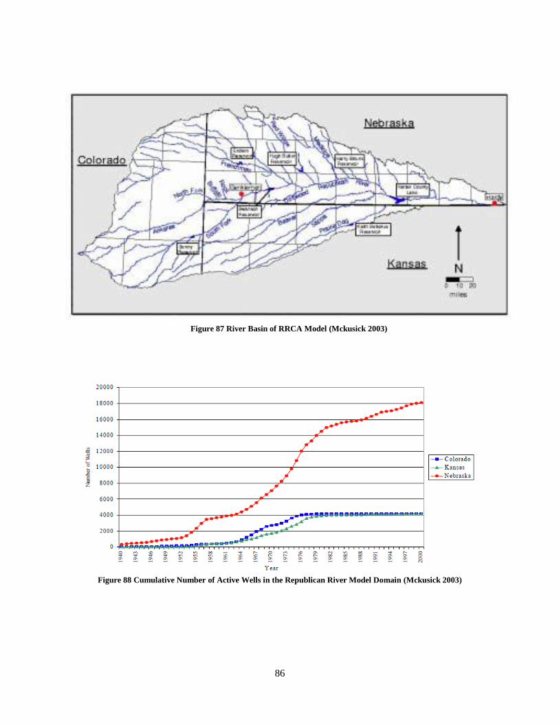
86

Figure 88 Cumulative Number of Active Wells in the Republican River Model Domain (Mckusick 2003)

Figure 87 River Basin of RRCA Model (Mckusick 2003)

87

Figure 89 Annual Pumping Volume for Perkins

Figure 90 Annual Pumping Volume for Chase

40000

90000

140000

190000

240000

290000

340000

1980 1985 1990 1995 2000 2005

An

nu

al P

um

pin

g V

olu

me

(ac

re-f

ee

t)

Year

perkins.pmp perkins.wel perkins.real

40000

90000

140000

190000

240000

290000

340000

1980 1985 1990 1995 2000 2005

An

nu

al P

um

pin

g V

olu

me

(ac

re-f

ee

t)

Year

chase.pmp chase.wel chase.real

88

Figure 91 Annual Pumping Volume for Dundy

Figure 92 Histogram of Difference between the Real Pumping Data and Modflow Data for Each Cell (1980-83)

40000

90000

140000

190000

240000

290000

340000

1980 1985 1990 1995 2000 2005

An

nu

al P

um

pin

g V

olu

me

(ac

re-f

ee

t)

Year

dundy.pmp dundy.wel dundy.real

89



90



91



92

Table 1 The Impact of Pumping Uncertainty on Parameter Estimation (Thiem and Theis)

Uncertain Thiem Theis

T T S T&S

Method1

s unbiased

Q bias=1.5 bias=1.6 bias=18 bias=1.5 (T)& 2(S)

Q&s bias=1.5 bias=1.6 bias=18 bias=1.5(T)&2(S)

Method2

s unbiased with enough data

Q unbiased bias=1.01;

cov=180

bias=35;

cov=100

bias=1,c.o.v.=140(T)

bias=1,c.o.v.=0.002(S)

Q&s

N=5 bias=1.16;

cov=230

bias=1.05;

cov=200

bias=40;

cov=140


bias=10,c.o.v.=3(S)

N=50 bias=1.01;

cov=200

bias=1.01;

cov=180

bias=35;

cov=60


bias=1,c.o.v.=0.1(S)

Table 2 The Impact of Pumping Uncertainty on Parameter Estimation in ZHB Model

(Drawdown Only)

drawdown only

T Sy k

Separated

Observation bias=1.2

c.o.v.=60

bias=1.5

c.o.v.=0.4

bias=100

c.o.v.=6000

Q bias=1.5

c.o.v.=600

bias=4

c.o.v.=5

bias=300

c.o.v.=12000

Q & obs bias=1.6

c.o.v.=700

bias=4.5

c.o.v.=15

bias=300

c.o.v.=12000

Simultaneously

Observation unbiased

c.o.v.=20

bias=1.4

c.o.v.=0.12

bias=40

c.o.v.=2000

Q unbiased

c.o.v.=40

bias=1.4

c.o.v.=0.15

bias=18

c.o.v.=100

Q & obs unbiased

c.o.v.=50

bias=1.8

c.o.v.=0.25

bias=100

c.o.v.=6000

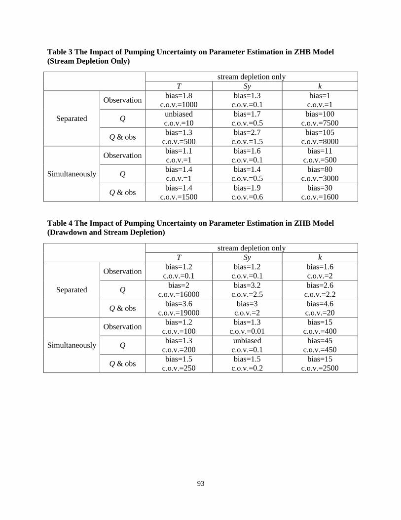
93


(Stream Depletion Only)

stream depletion only

T Sy k

Separated


c.o.v.=1000

bias=1.3

c.o.v.=0.1

bias=1

c.o.v.=1

Q unbiased

c.o.v.=10

bias=1.7

c.o.v.=0.5

bias=100

c.o.v.=7500

Q & obs bias=1.3

c.o.v.=500

bias=2.7

c.o.v.=1.5

bias=105

c.o.v.=8000

Simultaneously


c.o.v.=1

bias=1.6

c.o.v.=0.1

bias=11

c.o.v.=500

Q bias=1.4

c.o.v.=1

bias=1.4

c.o.v.=0.5

bias=80

c.o.v.=3000

Q & obs bias=1.4

c.o.v.=1500

bias=1.9

c.o.v.=0.6

bias=30

c.o.v.=1600


(Drawdown and Stream Depletion)

stream depletion only

T Sy k

Separated


c.o.v.=0.1

bias=1.2

c.o.v.=0.1

bias=1.6

c.o.v.=2

Q bias=2

c.o.v.=16000

bias=3.2

c.o.v.=2.5

bias=2.6

c.o.v.=2.2

Q & obs bias=3.6

c.o.v.=19000

bias=3

c.o.v.=2

bias=4.6

c.o.v.=20

Simultaneously


c.o.v.=100

bias=1.3

c.o.v.=0.01

bias=15

c.o.v.=400

Q bias=1.3

c.o.v.=200

unbiased

c.o.v.=0.1

bias=45

c.o.v.=450

Q & obs bias=1.5

c.o.v.=250

bias=1.5

c.o.v.=0.2

bias=15

c.o.v.=2500

94

Table 5 Difference between 'real' and 'wel' Date: (real-wel)/real

year Perkins Chase Dundy

1980 22.60% 4.65% 24.79%

1981 23.88% 11.58% 33.42%

1982 19.02% 13.52% 35.25%

1983 22.25% 16.11% 21.92%

1984 26.77% 9.29% 33.79%

1985 28.88% 13.79% 36.69%

1986 14.05% 9.01% 31.54%

1987 15.40% 11.08% 24.73%

1988 17.50% 9.17% 25.29%

1989 21.38% -0.07% 33.35%

1990 7.18% 7.83% 18.84%

1991 3.97% 4.26% 23.91%

1992 6.32% -1.65% 40.86%

1993 14.41% -36.11% 42.09%

1994 13.17% -8.35% 33.11%

1995 7.08% 0.22% 28.44%

1996 5.83% -3.28% 30.67%

1997 11.49% -1.27% 30.40%

1998 12.17% 0.04% 24.68%

1999 11.85% -13.46% 24.44%

2000 15.33% 3.17% 16.79%

2001 20.31% 9.17% 20.03%

2002 20.36% 9.46% 20.40%

2003 1.55% 1.01% 1.32%

2004 -2.78% 1.52% 3.78%

2005 -1.29% 0.69% 3.26%

2006 14.08% 7.54% 13.66%

Table 6 Mean and Variance of Differences (wel-real)

Year Mean Standard

Deviation Year Mean

Standard

Deviation Year Mean

Standard

Deviation

1980 -51.70 228.13 1989 -45.84 220.74 1998 -38.37 249.57

1981 -61.23 207.37 1990 -39.35 252.28 1999 -15.17 184.07

1982 -52.33 174.40 1991 -31.21 225.88 2000 -49.48 302.87

1983 -52.07 218.12 1992 -31.55 190.88 2001 -48.81 225.38

1984 -71.77 249.06 1993 -4.57 154.98 2002 -67.66 304.56

1985 -88.37 256.96 1994 -34.64 259.03 2003 -4.57 158.56

1986 -52.63 223.48 1994 -32.53 220.92 2004 -2.80 137.06

1987 -44.97 203.00 1996 -21.77 174.57 2005 -2.27 107.75

1988 -47.84 226.71 1997 -42.58 249.54 2006 -34.14 120.84

95

Bibliography

Beck, M. B. "Water quality modeling: A review of the analysis of uncertainty." Water Resources Research,

1987: 1393-1442.

Beven, Keith. "AManifesto for the Equifinality Thesis." Journal of Hyfrology, 2006: 18-36.

Bouwer, Herman. "Making Sense of the Interactions Between Groundwater and Streamflow: Lessons for

Water Masters and Adjudicators." Rivers, 1997: 19-31.

Butler, James J, Vitaly A. Zlotnik, and Ming-Shu Tsou. "Drawdown and Stream Depletion Produced by

Pumping in the Vicinity of a Partially Penetrating Stream." Ground Water, 2001: 651-659.

Butler, James J., and Ming-Shu Tsou. Mathematical Derivation of Drawdown and Stream Depletion

Produced by Pumping in the Vicinity of a Finite-Width Stream of Shallow Penetration. KGS OPEN

FILE REPORT, Lawrence, KS: Kansas Geological Survey, 2001.

Clement, T.P. A Modular Computer Code for Simulating Reactive Multispecies Transport in 3-Dimensional

Groundwater Systems. Richland, Washington: Pacific Northwest National Laboratory, 1997.

Doherty, John. "Model-Independent Parameter Estimation User Manual: 5th Edition." 2010.

Harbaugh, Arlen W. "MODFLOW-2005, The U.S. Geological Survey Modular Ground-Water Model-the

Ground-Water Flow Process." In U.S. Geological Survey Techniques and Methods 6–A16,

variously. 2005.

Hejberg, A.L., and J.C. Refsgaard. "Model uncertainty-parameter uncertainty versus conceptual models."

Water Science Technology, 2005: 177-186.

Lin, Zhulu. Theory for PEST Users. Athens, GA: University of Georgia, 2005.

Mckusick, Vincent L. "Final Report of The Special Master with Certificate of Adoption of RRCA

Groundwater Model." 2003.

Moreo, M.T., K.J. Halford, R.J. La Camera, and R.J. Laczniak. Estimated ground-water withdrawals from

the Death Valley regional flow system, Nevada and California, 1913–98. Water-Resources

Investigations Report, U.S. Geological Survey, 2003.

Neuman, S.P. "Calibration of distributed paramter groundwater flow models viewed as a multiple-

objective decision process under uncertainty." Water Resources Research, 1973: 1006-1021.

Pollock, David W. User’s Guide for MODPATH/MODPATH-PLOT, Version 3: A particle tracking post-

processing package for MODFLOW, the U. S. Geological Survey finite-difference ground-water .

Reston, Virginia: U. S. GEOLOGICAL SURVEY, 1994.

96

Ross, James L., Metin M. Ozbek, and George F. Pinder. "Aleatory and Epistemic Uncertainty in

Groundwater Flow and Transport Simulation." Water Resources Research, 2009.

Sudheer, K. P., G. Lakshmi, and I. Chaubey. "Application of a pseudo simulator to evaluate the sensitivity

of parameters in complex watershed models." Environmental Modelling Software , 2010: 135-

143.

Theis, Charles V. "The relation between the lowering of the piezometric surface and the rate and

duration of discharge of a well using ground-water storage." Transactions, American

Geophysical Union, 1935: 519-524.

Thiem, Günther. "Hydrologische methoden." Leipzig: J. M. Gebhardt, 1906: 56.

Wang, Herbert F., and Mary P. Anderson. Introdution to groundwater modeling: finite difference and

finite element methods. San Diego, California: Academic Press, Inc., 1982.

Wasserman, Larry. All of Statistics: A Concise Course in Statistical Inference. Pittsburgh, PA: Springer,

2010.

Yeh, William W-G. "Review of parameter indentification procedures in groundwater hydrology: the

inverse problem." Water Resources Research, 1986: 95-108.

Zhang, Hongxia, and Wen Song. "The current status and prospect of research on groundwater numerical

simulation." Water Conservancy Science and Technology and Economy, 2007: 794-796.

Zheng, Chunmiao, and P. Patrick Wang. "MT3DMS Documentation and User's Guide." 1999.

Zlotnik, Vitaly A., Huihua Huang, and James J. Butler. Evaluation of Strean Depletion Considering Finite

Stream Width, Shallow Penetration, and Properties of Streambed Sediments. Brisbane, Australia:

Water 99 Joint Congress, 1999.

Zouaoui, Faker; Wilson, James R. "Accounting for Input Model and Parameter Uncertainty in

Simulation." Techinical Report, 2002.

Documents

IMPACT OF UNCERTAIN INPUT ON PARAMETER …