Embed Size (px)
Citation preview
The Pennsylvania State University
The Graduate School
Department of Computer Science and Engineering
IMPACT OF SOFT ERRORS ON SCIENTIFIC SIMULATIONS
A Thesis in
Computer Science and Engineering
by
Sowmyalatha Bangalore Srinivasmurthy
c© 2011 Sowmyalatha Bangalore Srinivasmurthy
Submitted in Partial Fulfillmentof the Requirements
for the Degree of
Master of Science
December 2011
The thesis of Sowmyalatha Bangalore Srinivasmurthy was reviewed and approved*by the following:
Padma RaghavanProfessor of Computer Science and EngineeringDirector of Institute for CyberScienceThesis Adviser
Mahmut KandemirProfessor of Computer Science and Engineering
Raj AcharyaProfessor of Computer Science and EngineeringHead of the Department of Computer Science and Engineering
*Signatures are on file in the Graduate School
iii
Abstract
The trends in computing processor technology are driving toward multicores
through miniaturization that can pack many processors in a given chip area. This minia-
turization has led to a significant increase in the occurrence of soft errors, where a single
bit flip impacts the output of the computing system. This in-turn affects the performance
of the application running on the system. In this thesis, we attempt to understand and
characterize the impact of soft errors on scientific simulations. We consider the impact of
a single soft error on the widely used preconditioned conjugate gradient method (PCG),
an important kernel in such scientific simulations. We first show that a single error in
PCG can propagate through a sequence of sparse matrix vector multiplication (SpMV)
operations that form the core computations in PCG. Consequently, we demonstrate that
a single soft error in PCG can lead to performance degradation by factors of 200 or
more. Next, we consider the Community Earth System Model (CESM), an extensively
used coupled climate model that allows simulation of the earth’s climate system. Our
experimental results indicate that although the soft errors cause variations in the output
of the models, these variations are within the allowable range of perturbations. However,
the models are not robust enough and fail upon soft errors in the pointer data structures.
These results indicate the need for further study of the impact of soft errors on scientific
simulations and the need to develop methods for detection and mitigation.
iv
Table of Contents
List of Tables . . . . . . . . . . . . . . . . . . . . . . . . . . . . . . . . . . . . . . vi
List of Figures . . . . . . . . . . . . . . . . . . . . . . . . . . . . . . . . . . . . . vii
Acknowledgments . . . . . . . . . . . . . . . . . . . . . . . . . . . . . . . . . . . ix
Chapter 1. Introduction . . . . . . . . . . . . . . . . . . . . . . . . . . . . . . . . 1
Chapter 2. Related Research and Background . . . . . . . . . . . . . . . . . . . 4
2.1 Related Research . . . . . . . . . . . . . . . . . . . . . . . . . . . . . 4
2.1.1 Soft Error Detection . . . . . . . . . . . . . . . . . . . . . . . 4
2.1.2 Protection Against Soft Errors . . . . . . . . . . . . . . . . . 5
2.1.3 Soft Error Characterization . . . . . . . . . . . . . . . . . . . 6
2.2 Linear Solver Basics . . . . . . . . . . . . . . . . . . . . . . . . . . . 8
2.2.1 Conjugate Gradient . . . . . . . . . . . . . . . . . . . . . . . 9
2.3 Community Climate Models . . . . . . . . . . . . . . . . . . . . . . . 10
Chapter 3. Propagation of Soft Errors in Preconditioned Conjugate Gradient . . 13
3.1 Effect on Performance . . . . . . . . . . . . . . . . . . . . . . . . . . 14
3.2 Soft Error Propagation Pattern . . . . . . . . . . . . . . . . . . . . . 17
Chapter 4. Impact of Soft Errors on the Community Earth System Model . . . . 22
Chapter 5. Conclusion . . . . . . . . . . . . . . . . . . . . . . . . . . . . . . . . . 30

v
Bibliography . . . . . . . . . . . . . . . . . . . . . . . . . . . . . . . . . . . . . . 31
vi
List of Tables
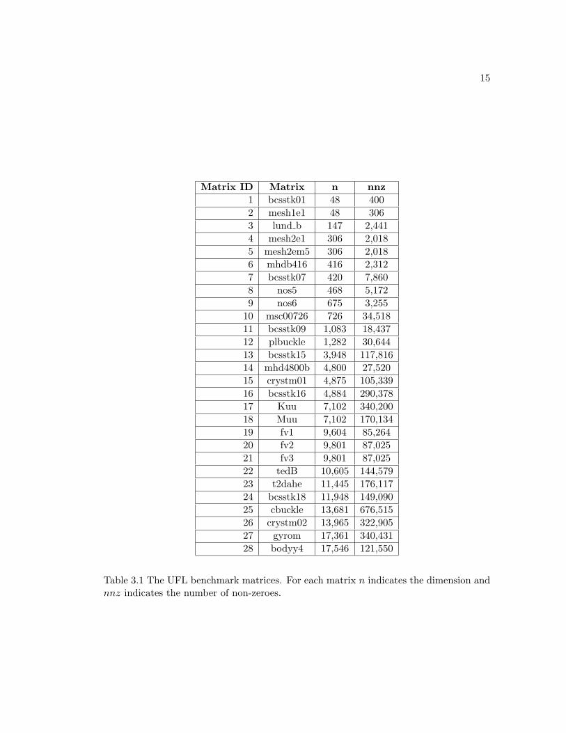
3.1 The UFL benchmark matrices. For each matrix n indicates the dimension
and nnz indicates the number of non-zeroes. . . . . . . . . . . . . . . . . 15

vii
List of Figures
2.1 Community Earth System Model . . . . . . . . . . . . . . . . . . . . . . 11
2.2 Atmosphere model workflow . . . . . . . . . . . . . . . . . . . . . . . . . 12
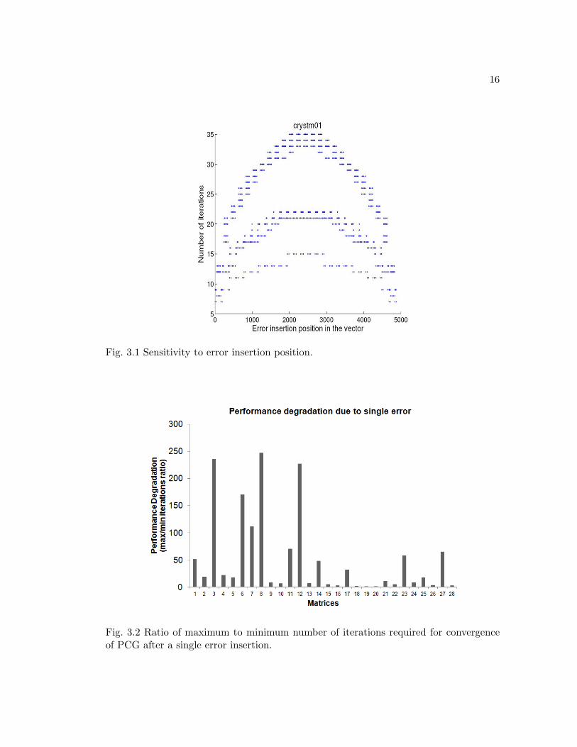
3.1 Sensitivity to error insertion position. . . . . . . . . . . . . . . . . . . . 16
3.2 Ratio of maximum to minimum number of iterations required for con-
vergence of PCG after a single error insertion. . . . . . . . . . . . . . . . 16
3.3 Sparsity structure of matrices (a) bcsstk34, (b) bcsstk35 and (c) pwtk. . 18
3.4 Sparse matrix A, vector y, and the sequence of SpMV operations on A
and y . . . . . . . . . . . . . . . . . . . . . . . . . . . . . . . . . . . . . 19
3.5 Intermediate tree representations (0 - 4 iterations) . . . . . . . . . . . . 19
3.6 Final tree representation . . . . . . . . . . . . . . . . . . . . . . . . . . . 20
3.7 Relative error in the Krylov subspace. . . . . . . . . . . . . . . . . . . . 21
4.1 Atmosphere model workflow with soft error insertion . . . . . . . . . . . 23
4.2 Effect of a single bit flip in the temperature field in the atmosphere model
on the mean energy . . . . . . . . . . . . . . . . . . . . . . . . . . . . . . 25
4.3 Effect of a single error in the temperature field in the atmosphere model
on surface pressure and heating rate . . . . . . . . . . . . . . . . . . . . 26
4.4 Effect of a single bit flip in the velocity field in the atmosphere model on
the mean energy . . . . . . . . . . . . . . . . . . . . . . . . . . . . . . . 27
viii
4.5 Effect of a single error in the velocity field in the atmosphere model on
surface pressure and heating rate . . . . . . . . . . . . . . . . . . . . . . 28

ix
Acknowledgments
I am immensely grateful and indebted to my thesis adviser and mentor, Dr.
Padma Raghavan, for her constant guidance and encouragement throughout my stay
at Penn State. I am indebted to her for the financial support made possible by the
generous funds from the National Science Foundation throughout my degree program,
without which, it would have been very difficult to complete my masters degree. I also
want to thank my husband and friend Manu Shantharam for all his support, patience
and encouragement that has kept me going. I am also very grateful to Dr. John Dennis
for his support during my work on the climate codes. The discussions were insightful
and enlightening, and has left me with a better understanding of the climate models. I
would also like to thank Dr. Mahmut Kandemir, my committee member for his insightful
commentary on my work.

x
Dedicated to my parents who have always been my inspiration.
1
Chapter 1
Introduction
Back in 1965, during the early years of the chip making Dr. Gordon Moore wrote
“The number of transistors incorporated in a chip will approximately double every 24
months” [30]. The prediction has indeed been true and it is expected to continue. How-
ever as the dimensions and operating voltages of electronic units shrink to accommodate
the increasing number of cores within a given chip area, there has been a significant
increase in the occurrence of soft errors [9], where a single bit flip can leave the output
of the computing system in a corrupt state. In this thesis we focus on the impact of soft
errors on scientific simulations that run on multicore systems.
Soft error or transient errors can be described as errors that lead to bit flips in
memory and errors in the logic circuit output that leaves the state of the computing sys-
tem corrupt. The errors can be caused by cosmic radiations [5], radiation from packaging
materials [8], as well as voltage fluctuation [5]. Soft-error rate in microprocessor logic has
become a reliability concern [32, 16, 38]. With increases in the transistor densities, the
soft error rates have been growing exponentially, with typical values ranging between
1k and 10k FIT/Mb [8] (FIT is failure per billion hours of operation). The 106,496
dual-processor compute node BlueGene/L, for example [11], is reported to experience
one soft error in its L1 cache every 4-6 hours induced due the radioactive decay in lead
solders. Michalak et al. [28] report that the ASCI Q experienced 27.7 CPU failures
2
per week due to radiation. There have been various studies to investigate their effects
on caches in single processor systems [39, 32, 23], on software systems [6, 38, 16], and
parallel applications [24].
Given the increase in the occurrence of soft errors, various techniques have been
suggested and implemented to overcome these effects. But with technology moving
towards the chip multiprocessors, it is becoming important to study the behavior of these
errors in today’s systems. With levels of memory and caches well protected against the
insertion of soft errors, the processor itself is still left susceptible. Soft errors induced at
the processor level go untraced and can affect the final output of the application that
was running during that period. This poses a reliability challenge in the field of high
performance computing as most of the applications have long execution time. A majority
of large-scale scientific applications run on supercomputers. Super computers consists of
multiple multicores, thus increasing the occurrence of the soft errors in these systems.
A majority of the long running scientific applications involve partial differential
equation (PDE) based systems, such as those found in heat diffusion, computational fluid
dynamics (CFD) and structural mechanics. Such applications typically use software tool
kits such as PETSc [26], in conjunction with iterative linear solver packages like Hypre
[14] and Trilinos [19]. The basic underlying computation in these software packages is a
sequence of sparse matrix vector multiplication (SpMV) operations of the form y ← A.v
that are performed iteratively within an iterative sparse linear solver such as conjugate
gradient (CG) and its preconditioned forms. Reliable and accurate fast simulations can
be viewed as depending on the performance of the SpMV kernel and the propagation of
numerical attributes through relevant sequence of SpMV operations.

3
In this thesis, we first present the effect of soft errors on performance of iterative
linear solvers, in particular CG and preconditioned CG (PCG) . Our experiments indicate
that a single soft error has the potential to degrade the performance of PCG by as much
as a factor of 200x. We also attempt to characterize the propagation pattern of soft errors
in the SpMV kernel within PCG. Next, we present a case study on a real life scientific
application, the Community Earth System Model (CESM), a community climate code.
We conclude that the climate codes are robust when the data in physics based model
are corrupted by single soft errors but fail when pointers to the data are corrupted.
The thesis is organized as follows. Chapter 2 first begins with a brief overview
of the recent research related to soft error detection, and characterization followed by a
discussion of the basic concepts of linear solvers and community climate models. Chapter
3 explores the effect of the sparsity pattern of a matrix on the propagation of a single
soft error and presents the impact of a soft error on the performance of an iterative linear
solver. Chapter 4 presents a case study of the impact of soft errors on community climate
models. Finally, Chapter 5 contains a summary of the thesis with brief comments on
future research directions.
4
Chapter 2
Related Research and Background
In this chapter, we provide a brief overview of the related research done in the
area of soft error detection, mitigation and characterization. Later in the chapter, we
provide basic background information about the linear solvers and the conjugate gradient
method, an iterative linear solver that we use in our experiments. We also give a short
overview of the Community Earth System Model, a community climate model used as a
case study in the thesis.
2.1 Related Research
The research in the field of soft errors can be categorized into 3 areas: (i) soft
error detection [16, 38, 33, 20] which involves online or static methods of detecting soft
errors, (ii) protection against soft error [7, 29, 22, 35] which involves selective protection
of the systems against the soft errors using external techniques, and (iii) soft error
characterization [40, 31, 15] where the behavior of the application or system under soft
error attack is understood to come up with protection and mitigation schemes based on
the characterization.
2.1.1 Soft Error Detection
The first area of an error detection technique called fingerprinting is proposed
by Smolens et al. [16], which detects differences in execution across a dual modular
5
redundant (DMR) processor pair. In fingerprinting a processor’s execution history is
summarized in a hash-based signature. The comparison of their fingerprints expose the
differences between two mirrored processors. Fingerprinting is based on the schemes
used for fault tolerance techniques. This technique needs special hardware modifications
to the processor pipeline.
Software based detection techniques have been developed to detect soft error
[33, 20] to avoid large hardware overhead. Rebaudengo et al. [33] propose a technique
that automatically transforms programs written in any high level language to be able
to detect most of the errors affecting data and code. The proposed transformation rules
can be implemented into a compiler as a pre-processing phase, thus making it com-
pletely transparent to the programmer. Hu et al. [20] focus on utilizing the compilers
to duplicate instructions for error detection in the VLIW datapath. The instruction du-
plication mechanism is further supported by a hardware enhancement for efficient result
verification, thus avoiding the need for additional comparison instructions. In their pro-
posed approach, the trade off between performance, reliability and energy consumption
is achieved through the compiler by determining degree of instruction duplication.
2.1.2 Protection Against Soft Errors
The next area of research in this field focus on protecting processors from soft
errors. SHIELD [29] is an architecture that increases the resistance of register files to
soft errors. Based on the observation that the data stored in a register is only useful
for a small fraction of the lifetime of the registers and that not all registers are equally
vulnerable to soft errors, SHIELD selectively protects registers by storing the ECCs of
6
the most vulnerable registers while they contain useful data, and checks their integrity
off the critical path. Latif et al. [22] assessed the benefits of inherent error detection
and optional error correction on the software side. They study programming patterns
that exhibit properties for inherent detection of transient faults compared to techniques
that use instruction duplication, their technique can, not only save execution time but
reduce code size.
2.1.3 Soft Error Characterization
Another area of research deals with soft error characterization. Zhang et al.
[40] made the first attempt to characterize microarchitecture soft error vulnerabilities
across the stacked chip layers under 3D integration technologies. They use models and
simulations that capture soft error physical mechanism and circuit/architecture level
impact. Their study reveals the opportunities of leveraging 3D integration to achieve
enhanced reliability. The second feature enables the deployment of error resilience device
techniques to achieve a reliability target while minimizing manufacturing cost. They also
propose a set of microarchitecture techniques, which can effectively exploit the reliability
benefits offered by 3D technologies.
There have also been studies that focus on the soft error vulnerability of specific
applications. Lu and Reed [5] evaluate the soft error vulnerability of three MPI appli-
cations. They show the correlation between error injection sites and the application’s
vulnerability to such errors. Skarin, et al. [37] evaluate the soft error vulnerability of a
brake-by-wire system for automobiles using a similar approach. Although both studies
thoroughly evaluate the soft error vulnerability of the selected target application, they
7
provide little insight about the vulnerability of other applications. This makes any gen-
eralizing of the results difficult. Alternatively, Messer et al. [27] evaluate the soft error
vulnerability of a realistic software stack. They show the soft error properties of other
applications running on the same OS and the same application running on different OSs.
In this thesis we focus on the impact of soft errors on scientific applications, in
particular sparse linear solver preconditioned conjugate gradient method. There has
been recent interest in understanding this as well as the protection of these applications
against soft errors. Bronevetsky et al.[11] report observations on the effect of soft errors
on iterative solvers like, CG, preconditioned Richardson, and Chebyshev methods in
SparseLib [13]. Based on the experimental observations, the paper the impact of soft
errors as (i) no effect, (ii) silent error, (iii) application hangs observations, and (iv)
application crashes. The paper also proposes and evaluates several soft error detection
and tolerance schemes, like, residual tracking, checkpointing and data structure encoding
that could potentially lead to significant improvements in the reliability of these libraries.
Malkowski et al. [25] consider PCG and GMRES and they focus on utilizing the manner
in which the coefficient matrix A is resident in L1 and L2 caches in these methods.
They use the concept of vulnerable time to propose and evaluate energy and reliability
tradeoffs for two schemes, for adaptively turn-off the Error Correction Code (ECC) for
L1 cache and L2 caches. They assume little or no cache reuse for the vector v and
therefore is not protected. The data structures having higher resident time in the caches
than their corresponding vulnerable time, are protected.
8
2.2 Linear Solver Basics
There are basically two classes of methods to solve a linear system of the form
Ax = b (where A is a n× n coefficient matrix, b is an n× 1 known vector and x is an
n× 1 vector of unknowns): (i) direct methods (ii) iterative methods,
Direct methods attempt to solve the problem using a finite sequence of operations.
These methods yield an exact solution in the absence of rounding errors. They are
typically used to solve moderately sized systems with a dense coefficient matrix. Gaussian
elimination is one of the most widely used methods to solve such a system. It uses the
the idea of modifying the matrix into an upper triangular form (Ux = b′ where b′ is
the corresponding change in the known right hand side vector) while still maintaining
the solution to the original system. The obtained triangular system is then solved by
back substitution. The triangularization of the coefficient matrix A is achieved by using
the LU factorization method, where L stands for lower triangular matrix and U stands
for upper triangular matrix. In LU factorization, the coefficient matrix is factorized
into an upper and lower triangular matrices (A = LU) and then solved using back
substitution successively on the two triangular matrices L and U to solve the system.
Direct methods can be used on sparse matrices as well. A modified LU factorization
algorithm that attempts to find sparse factors L and U could be used here. The number
of non-zero elements determine the computational cost of these algorithms in the case
of sparse systems. The runtime also depends on the sparsity structure of the coefficient
matrix. In the case of a dense coefficient matrix, the runtime depends only on size; and
is independent of data, structure, or sparsity.
9
Indirect or iterative methods [34] aim to yield a sequence of improving approx-
imate solutions for a class of problems. An iterative method uses an initial guess and
generates successive approximations to a solution. The rate at which an iterative method
converges depends greatly on the eigen spectrum [18] of the coefficient matrix. Iterative
methods usually involve a transformation matrix called a preconditioner that transforms
the coefficient matrix into a matrix with a more favorable spectrum. A good precondi-
tioner improves the convergence of the iterative method. Without a preconditioner the
iterative method may fail to converge.
2.2.1 Conjugate Gradient
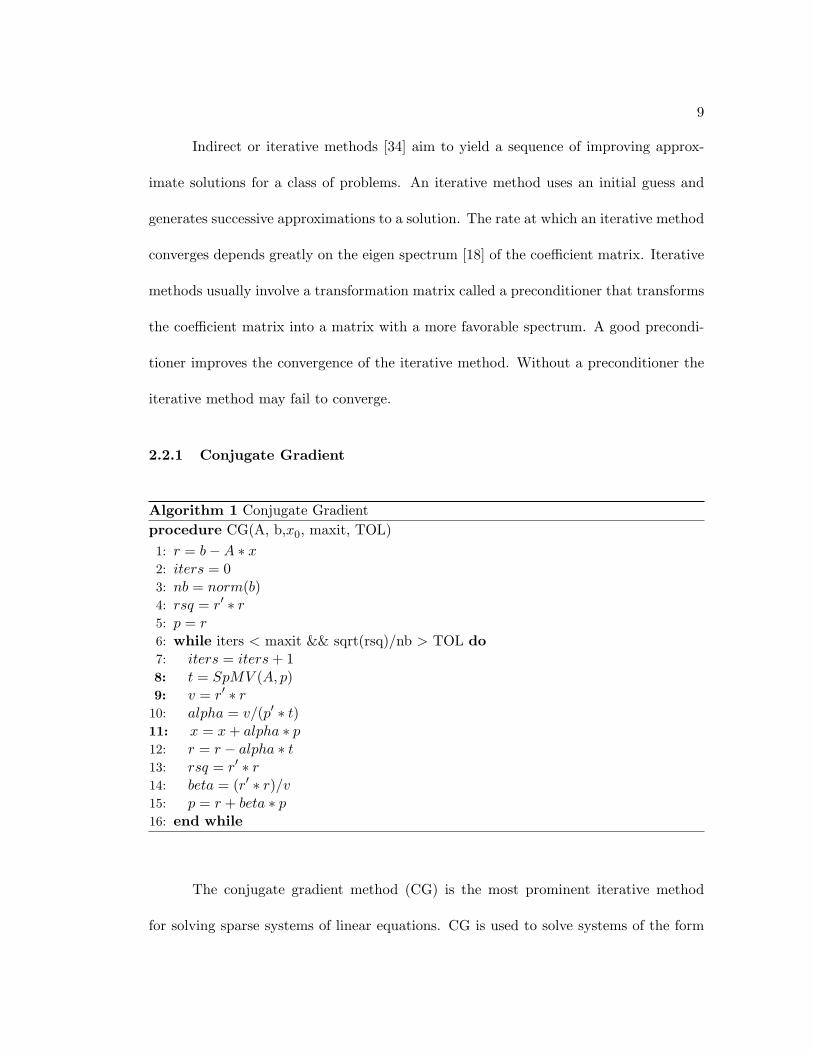
Algorithm 1 Conjugate Gradientprocedure CG(A, b,x0, maxit, TOL)1: r = b−A ∗ x2: iters = 03: nb = norm(b)4: rsq = r′ ∗ r5: p = r6: while iters < maxit && sqrt(rsq)/nb > TOL do7: iters = iters+ 18: t = SpMV (A, p)9: v = r′ ∗ r
10: alpha = v/(p′ ∗ t)11: x = x+ alpha ∗ p12: r = r − alpha ∗ t13: rsq = r′ ∗ r14: beta = (r′ ∗ r)/v15: p = r + beta ∗ p16: end while
The conjugate gradient method (CG) is the most prominent iterative method
for solving sparse systems of linear equations. CG is used to solve systems of the form

10
Ax = b, where x is an unknown vector, b is a known vector, and A is a known, symmetric,
positive-definite matrix. These systems arise in many scientific settings, such as finite
difference and finite element methods for solving partial differential equations, structural
analysis and circuit analysis. CG works on the vectors represented by an SpMV sequence,
span(v,Av, . . . Anv) to find a solution for the linear system, where, A is the coefficient
matrix and v is the initial residual vector. This span of vectors is known as Krylov
subspace [17]. Hence each iteration of CG requires a SpMV operation of the form
t← A.p [line 9 in Algorithm 1]. Thus the SpMV operation dominates the computation
time of CG. In many cases, naive CG takes a long time to converge to a solution. Hence,
preconditioning is necessary to ensure fast convergence of the CG algorithm. This variant
of CG with the preconditioning stage is called preconditioned conjugate gradient (PCG),
and is a widely used linear iterative solver in scientific applications.
2.3 Community Climate Models
The Community Earth System Model (CESM) [2] is a fully-coupled, global cli-
mate model aimed to provide state-of-the-art computer simulations of the Earth’s past,
present, and future climate states. CESM is sponsored by the National Science Foun-
dation (NSF) and the U.S. Department of Energy (DOE). CESM is maintained by the
Climate and Global Dynamics Division (CGD) at the National Center for Atmospheric
Research (NCAR).
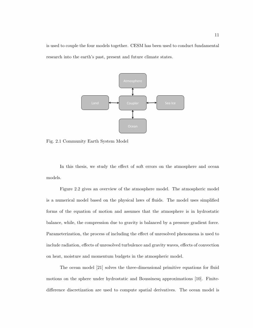
Figure 2.1 illustrates the Community Earth System Model. The model is com-
posed of four separate model, atmosphere, ocean, land surface and sea-ice. These models
are used to simultaneously simulate the earth’s climate. The central coupler component
11
is used to couple the four models together. CESM has been used to conduct fundamental
research into the earth’s past, present and future climate states.
Atmosphere
Land
Ocean
SeaIceCoupler
Fig. 2.1 Community Earth System Model
In this thesis, we study the effect of soft errors on the atmosphere and ocean
models.
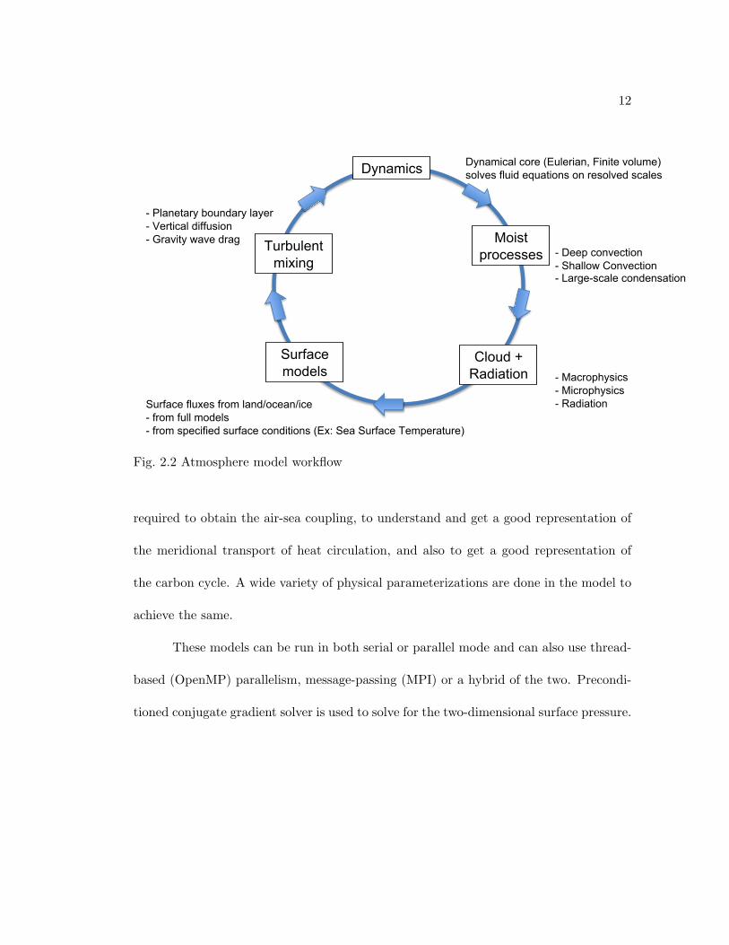
Figure 2.2 gives an overview of the atmosphere model. The atmospheric model
is a numerical model based on the physical laws of fluids. The model uses simplified
forms of the equation of motion and assumes that the atmosphere is in hydrostatic
balance, while, the compression due to gravity is balanced by a pressure gradient force.
Parameterization, the process of including the effect of unresolved phenomena is used to
include radiation, effects of unresolved turbulence and gravity waves, effects of convection
on heat, moisture and momentum budgets in the atmospheric model.
The ocean model [21] solves the three-dimensional primitive equations for fluid
motions on the sphere under hydrostatic and Boussinesq approximations [10]. Finite-
difference discretization are used to compute spatial derivatives. The ocean model is
12
Dynamics
Moist processes
Cloud + Radiation
Surface models
Turbulent mixing
- Deep convection - Shallow Convection - Large-scale condensation
- Macrophysics - Microphysics - Radiation Surface fluxes from land/ocean/ice
- from full models - from specified surface conditions (Ex: Sea Surface Temperature)
- Planetary boundary layer - Vertical diffusion - Gravity wave drag
Dynamical core (Eulerian, Finite volume) solves fluid equations on resolved scales
Fig. 2.2 Atmosphere model workflow
required to obtain the air-sea coupling, to understand and get a good representation of
the meridional transport of heat circulation, and also to get a good representation of
the carbon cycle. A wide variety of physical parameterizations are done in the model to
achieve the same.
These models can be run in both serial or parallel mode and can also use thread-
based (OpenMP) parallelism, message-passing (MPI) or a hybrid of the two. Precondi-
tioned conjugate gradient solver is used to solve for the two-dimensional surface pressure.
13
Chapter 3
Propagation of Soft Errors in
Preconditioned Conjugate Gradient
In this chapter, we explore the effect of sparsity pattern of a sparse matrix on
propagation of single soft error during the SpMV operation and present the impact of a
soft error on the performance of an iterative linear solver, in partiular PCG. To facilitate
better understanding, we first provide notation and terminology used in this chapter.
Notation and Terminology. Vectors and matrices are represented as italicized
lowercase and uppercase letters respectively. For example, vector y and matrix A. Unless
mentioned otherwise, vectors are of size n × 1 and matrices are of size n × n. The ith
element of a vector y is represented as yi. Following are the definitions of the terms we
use in this chapter.
Sparsity pattern of a sparse matrix is the connectivity structure of the sparse matrix in
its graph representation.
Krylov subspace generated by A and r is equal to span{r,Ar, A2r ... Akr }.
Consider a sparse linear system, Ax = b, where, A is a sparse symmetric positive
definite coefficient matrix, b and x are known and unknown vectors, respectively of size
n×1. Let the conjugate gradient (CG) method solve this system. The CG method works
on the vectors represented by a SpMV sequence (y ← Av; v ← y), span(v,Av, . . . Anv) to
find a solution for the linear system, where v is the initial residual vector. The resultant
vector is written back and used in the next iteration. Therefore, across the iterations
14
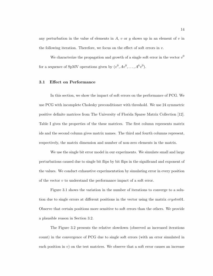
any perturbation in the value of elements in A, v or y shows up in an element of v in
the following iteration. Therefore, we focus on the effect of soft errors in v.
We characterize the propagation and growth of a single soft error in the vector v0
for a sequence of SpMV operations given by (v0, Av0, . . . , Akv0).
3.1 Effect on Performance
In this section, we show the impact of soft errors on the performance of PCG. We
use PCG with incomplete Cholesky preconditioner with threshold. We use 24 symmetric
positive definite matrices from The University of Florida Sparse Matrix Collection [12].
Table I gives the properties of the these matrices. The first column represents matrix
ids and the second column gives matrix names. The third and fourth columns represent,
respectively, the matrix dimension and number of non-zero elements in the matrix.
We use the single bit error model in our experiments. We simulate small and large
perturbations caused due to single bit flips by bit flips in the significand and exponent of
the values. We conduct exhaustive experimentation by simulating error in every position
of the vector v to understand the performance impact of a soft error.
Figure 3.1 shows the variation in the number of iterations to converge to a solu-
tion due to single errors at different positions in the vector using the matrix crystm01.
Observe that certain positions more sensitive to soft errors than the others. We provide
a plausible reason in Section 3.2.
The Figure 3.2 presents the relative slowdown (observed as increased iterations
count) in the convergence of PCG due to single soft errors (with an error simulated in
each position in v) on the test matrices. We observe that a soft error causes an increase
15
Matrix ID Matrix n nnz1 bcsstk01 48 4002 mesh1e1 48 3063 lund b 147 2,4414 mesh2e1 306 2,0185 mesh2em5 306 2,0186 mhdb416 416 2,3127 bcsstk07 420 7,8608 nos5 468 5,1729 nos6 675 3,255
10 msc00726 726 34,51811 bcsstk09 1,083 18,43712 plbuckle 1,282 30,64413 bcsstk15 3,948 117,81614 mhd4800b 4,800 27,52015 crystm01 4,875 105,33916 bcsstk16 4,884 290,37817 Kuu 7,102 340,20018 Muu 7,102 170,13419 fv1 9,604 85,26420 fv2 9,801 87,02521 fv3 9,801 87,02522 tedB 10,605 144,57923 t2dahe 11,445 176,11724 bcsstk18 11,948 149,09025 cbuckle 13,681 676,51526 crystm02 13,965 322,90527 gyrom 17,361 340,43128 bodyy4 17,546 121,550
Table 3.1 The UFL benchmark matrices. For each matrix n indicates the dimension andnnz indicates the number of non-zeroes.
16
Fig. 3.1 Sensitivity to error insertion position.
Fig. 3.2 Ratio of maximum to minimum number of iterations required for convergenceof PCG after a single error insertion.
17
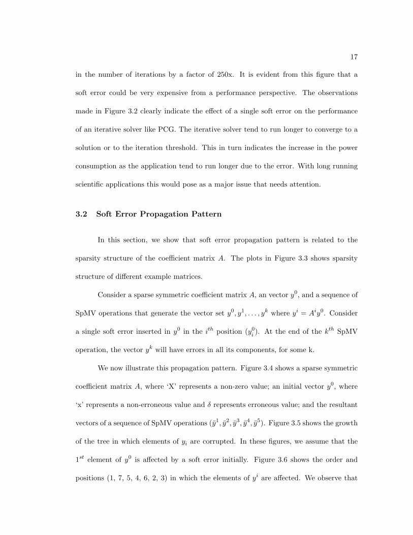
in the number of iterations by a factor of 250x. It is evident from this figure that a
soft error could be very expensive from a performance perspective. The observations
made in Figure 3.2 clearly indicate the effect of a single soft error on the performance
of an iterative solver like PCG. The iterative solver tend to run longer to converge to a
solution or to the iteration threshold. This in turn indicates the increase in the power
consumption as the application tend to run longer due to the error. With long running
scientific applications this would pose as a major issue that needs attention.
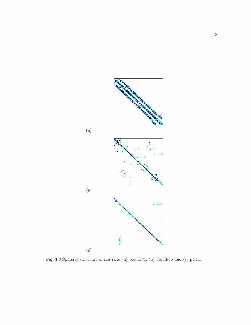
3.2 Soft Error Propagation Pattern
In this section, we show that soft error propagation pattern is related to the
sparsity structure of the coefficient matrix A. The plots in Figure 3.3 shows sparsity
structure of different example matrices.
Consider a sparse symmetric coefficient matrix A, an vector y0, and a sequence of
SpMV operations that generate the vector set y0, y1, . . . , yk where yi = Aiy0. Consider
a single soft error inserted in y0 in the ith position (y0i). At the end of the kth SpMV
operation, the vector yk will have errors in all its components, for some k.
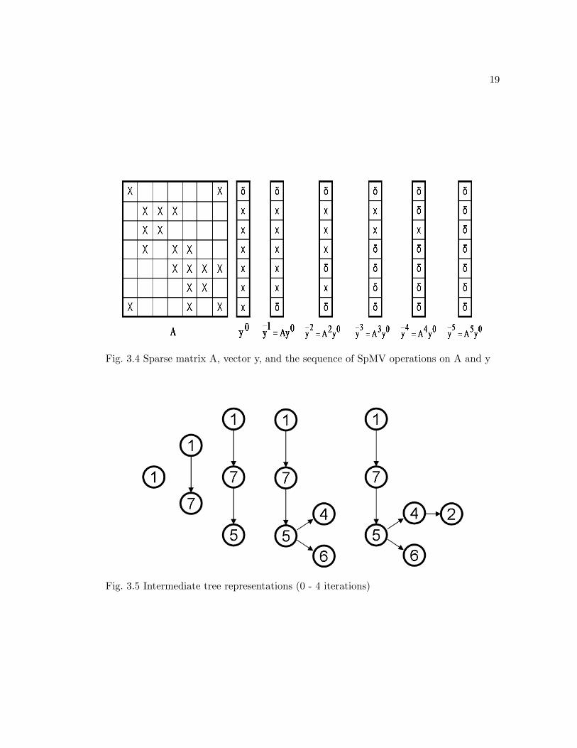
We now illustrate this propagation pattern. Figure 3.4 shows a sparse symmetric
coefficient matrix A, where ‘X’ represents a non-zero value; an initial vector y0, where
‘x’ represents a non-erroneous value and δ represents erroneous value; and the resultant
vectors of a sequence of SpMV operations (y1, y2, y3, y4, y5). Figure 3.5 shows the growth
of the tree in which elements of yi are corrupted. In these figures, we assume that the
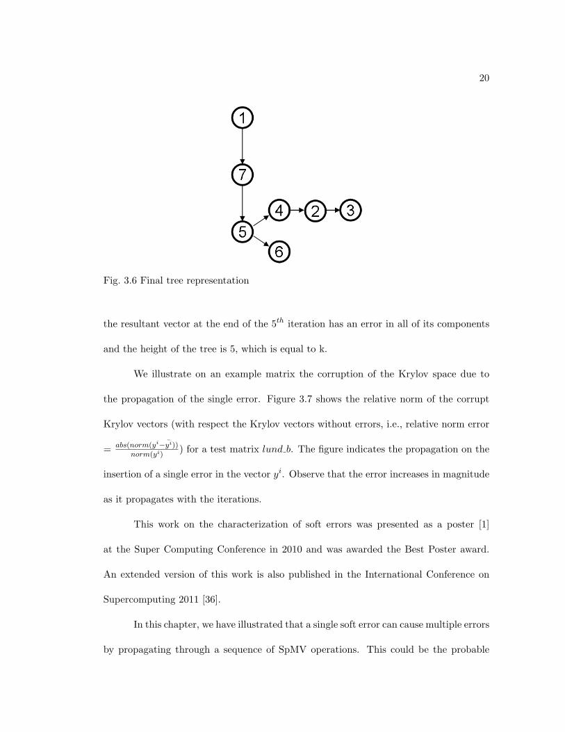
1st element of y0 is affected by a soft error initially. Figure 3.6 shows the order and
positions (1, 7, 5, 4, 6, 2, 3) in which the elements of yi are affected. We observe that
18
(a)
(b)
(c)
Fig. 3.3 Sparsity structure of matrices (a) bcsstk34, (b) bcsstk35 and (c) pwtk.
19
Fig. 3.4 Sparse matrix A, vector y, and the sequence of SpMV operations on A and y
Fig. 3.5 Intermediate tree representations (0 - 4 iterations)
20
Fig. 3.6 Final tree representation
the resultant vector at the end of the 5th iteration has an error in all of its components
and the height of the tree is 5, which is equal to k.
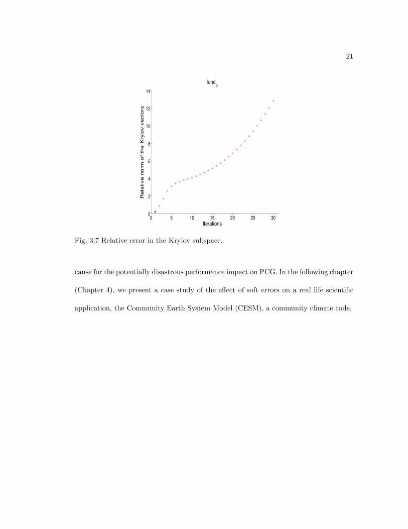
We illustrate on an example matrix the corruption of the Krylov space due to
the propagation of the single error. Figure 3.7 shows the relative norm of the corrupt
Krylov vectors (with respect the Krylov vectors without errors, i.e., relative norm error
= abs(norm(yi−yi))
norm(yi)) for a test matrix lund b. The figure indicates the propagation on the
insertion of a single error in the vector yi. Observe that the error increases in magnitude
as it propagates with the iterations.
This work on the characterization of soft errors was presented as a poster [1]
at the Super Computing Conference in 2010 and was awarded the Best Poster award.
An extended version of this work is also published in the International Conference on
Supercomputing 2011 [36].
In this chapter, we have illustrated that a single soft error can cause multiple errors
by propagating through a sequence of SpMV operations. This could be the probable
21
Fig. 3.7 Relative error in the Krylov subspace.
cause for the potentially disastrous performance impact on PCG. In the following chapter
(Chapter 4), we present a case study of the effect of soft errors on a real life scientific
application, the Community Earth System Model (CESM), a community climate code.

22
Chapter 4
Impact of Soft Errors on
the Community Earth System Model
The Community Earth System Model (CESM) is a coupled climate model that
allows simulation of the earth’s climate system. The model is a long running scientific
application that is run on multiple cores. Any error that affects the application can
potentially lead to loss of performance as well as power. This makes the study of the
effect of soft errors on this applications useful in building a more robust application.
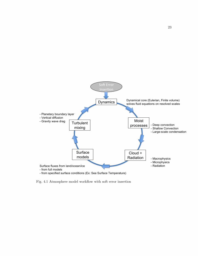
We use the atmosphere model (CAM) and ocean model (POP) for our experi-
ments. Figure 4.1 illustrates the location of the error insertion in the atmosphere model.
The experiments are conducted in the spectral transform dynamical core of the model.
We conduct experiments with single bit error insertion model, wherein, the error in
simulated by flipping a single bit of the exponent or significand in the target variable. The
error inserted is used to simulate a large or small change in magnitude of the variables.
We also simulate a change in sign of the value by flipping the sign bit. In our experiments,
we run the model on 32 cores of the Kraken [4] and Frost [3] for a model time of 1 month
with a resolution of T31 gx3v5. The resolution can be understood as approximately 3.75
degree latitudinal resolution with longitudinal resolution of 3.6 degrees. We analyze the
values of the global integrals given out by the model to determine the effect of the error
on the output. The global integrals that we use are mean energy going into physics,
mean energy coming out of physics, heating rate, and surface pressure.
23
Dynamics
Moist processes
Cloud + Radiation
Surface models
Turbulent mixing
- Deep convection - Shallow Convection - Large-scale condensation
- Macrophysics - Microphysics - Radiation Surface fluxes from land/ocean/ice
- from full models - from specified surface conditions (Ex: Sea Surface Temperature)
- Planetary boundary layer - Vertical diffusion - Gravity wave drag
Dynamical core (Eulerian, Finite volume) solves fluid equations on resolved scales
So#ErrorInser+on
Fig. 4.1 Atmosphere model workflow with soft error insertion
24
We first observe the effects of the single error in data, in the PCG solver, within
the finite volume model of the atmosphere model. We do not observe any change in the
output as a result of this error. Analysis showed that the PCG solver within the model
have a lower threshold for the number of iterations to convergence. The solvers discards
instances where the solution does not converge within the allowed threshold.
We next investigate the effect of single soft errors in the physical variables like
temperature, velocity and volume within the atmosphere model.
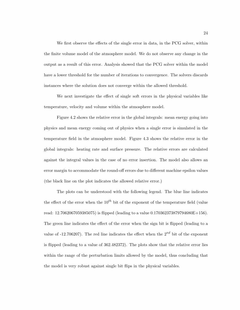
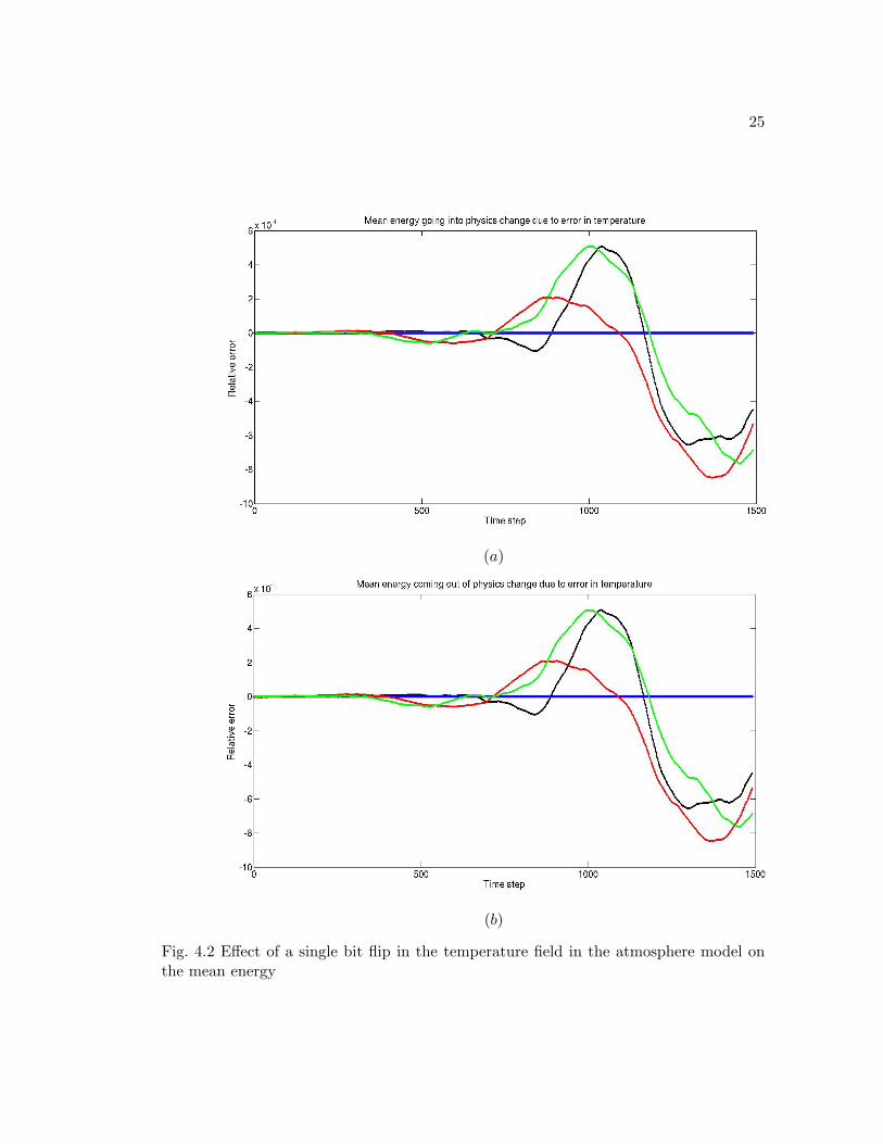
Figure 4.2 shows the relative error in the global integrals: mean energy going into
physics and mean energy coming out of physics when a single error is simulated in the
temperature field in the atmosphere model. Figure 4.3 shows the relative error in the
global integrals: heating rate and surface pressure. The relative errors are calculated
against the integral values in the case of no error insertion. The model also allows an
error margin to accommodate the round-off errors due to different machine epsilon values
(the black line on the plot indicates the allowed relative error.)
The plots can be understood with the following legend. The blue line indicates
the effect of the error when the 10th bit of the exponent of the temperature field (value
read: 12.7062067059385075) is flipped (leading to a value 0.170362373879794680E+156).
The green line indicates the effect of the error when the sign bit is flipped (leading to a
value of -12.706207). The red line indicates the effect when the 2nd bit of the exponent
is flipped (leading to a value of 362.482372). The plots show that the relative error lies
within the range of the perturbation limits allowed by the model, thus concluding that
the model is very robust against single bit flips in the physical variables.
25
(a)
(b)
Fig. 4.2 Effect of a single bit flip in the temperature field in the atmosphere model onthe mean energy
26
(c)
(d)
Fig. 4.3 Effect of a single error in the temperature field in the atmosphere model onsurface pressure and heating rate
27
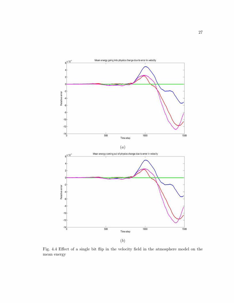
(a)
(b)
Fig. 4.4 Effect of a single bit flip in the velocity field in the atmosphere model on themean energy
28
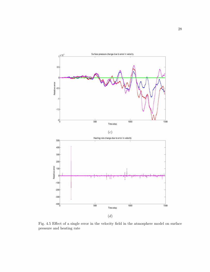
(c)
(d)
Fig. 4.5 Effect of a single error in the velocity field in the atmosphere model on surfacepressure and heating rate
29
Similar results are observed when a single error was inserted in the velocity compo-
nent of the atmosphere model. Figure 4.4 shows the relative error in the global integrals:
mean energy going into physics and mean energy coming out of physics and Figure 4.5
shows the relative error in the global integrals: heating rate and surface pressure. As
before, the relative errors are calculated against the integral values in the case of no
error insertion. The error margin allowed by the model is marked with the cyan line.
The red line indicates the effect of the error when the 10th bit of the exponent of the
temperature field (value read: -1.35923482838048648 ) is flipped (leading to a value
0.101376364837761051E-153). The blue line indicates the effect of the error when the
sign bit is flipped (leading to a value of 1.35923482838048648). The green line indicates
the effect when the sign bit of the maximum value in the velocity component is flipped
(leading to a value of 362.482372).
We also conducted experiments using the ocean model. Here the error insertion
was done into the time management module. The error was inserted into the pointers
to the data unlike in the data in the atmosphere model. The ocean model consistently
fails with segmentation faults.
On analyzing the behavior of the models to data corruption and the behavior
on pointer corruption we conclude that the models are robust against single bit data
corruptions in the physics based model. The models are deterministic and are capable
of factoring out any reliability issue due to single bit data corruption. But the models
are not robust enough to handle errors in the pointer data structures and result in
segmentation faults. The case study was brief and is not complete. The study of the
effects of the errors on the climate models will be continued as a part of the future work.
30
Chapter 5
Conclusion
In this thesis, we have demonstrated that soft errors can negatively impact long
running scientific applications on advanced computer hardware. We study the impact of
soft errors on the preconditioned conjugate gradient method (PCG), which is an iterative
linear solver that is at the core of many such applications. Our results show that a single
soft error has the potential to degrade the performance of PCG by a factor of 200 or
more. We also study the effect of soft errors on the Community Earth System Model
(CESM), a widely used scientific application to conduct fundamental research into the
earth’s past, present and future climate states. Our study on CESM indicates that the
physics based models are robust against single bit data corruptions. However, the models
are not robust enough and fail to handle such errors in the pointer data structures. The
results in this thesis indicate the need for further study of the impact of soft errors on
scientific simulations and the need to develop methods for detection and mitigation.
31
Bibliography
[1] http://sc10.supercomputing.org/files/sc10awardshpcnewsrelease.html.
[2] http://www.cesm.ucar.edu/.
[3] http://www.nar.ucar.edu/2009/cisl/1comp/1.3.12.tgops.php.
[4] http://www.nics.tennessee.edu/computing-resources/kraken.
[5] R.C. Baumann. Radiation-induced soft errors in advanced semiconductor technolo-gies. volume 5, pages 305 – 316, sept. 2005.
[6] Philippe Bernadat and Durga Devi Mannaru. Susceptibility of commodity systemsand software to memory soft errors. volume 53, pages 1557–1568, Washington,DC, USA, 2004. IEEE Computer Society. Member-Messer, Alan and Member-Fu,Guangrui and Member-Chen, Deqing and Member-Dimitrijevic, Zoran and Member-Lie, David and Member-Riska, Alma and Member-Milojicic, Dejan.
[7] J. Blome, S. Mahlke, D. Bradley, and K. Flautner. A microarchitectural analysis ofsoft error propagation in a production-level embedded microprocessor. In Proceed-ings of the 1st Workshop on Architectural Reliability, 38th International Symposiumon Microarchitecture, Barcelona, Spain, 2005.
[8] Daniel L. Boley, Richard P. Brent, Gene H. Golub, and Franklin T. Luk. Algorithmicfault tolerance using the lanczos method. volume 13, pages 312–332, Philadelphia,PA, USA, January 1992. Society for Industrial and Applied Mathematics.
[9] Shekhar Borkar. Introduction to panel discussion probabilistic & statistical design- the wave of the future. In VLSI-SoC, 2006.
[10] J. Boussinesq. Thorie de l’intumescence liquide, applele onde solitaire ou de trans-lation, se propageant dans un canal rectangulaire. page 755759, 1871.
[11] Greg Bronevetsky and Bronis de Supinski. Soft error vulnerability of iterative linearalgebra methods. In Proceedings of the 22nd annual international conference onSupercomputing, ICS ’08, pages 155–164, New York, NY, USA, 2008. ACM.
[12] T. Davis. The University of Florida Sparse Matrix Collection. NA Digest, 97, 1997.
[13] Jack Dongarra, Andrew Lumsdaine, Xinhui Niu, Roldan Pozo, and Karin Reming-ton. Sparse matrix libraries in c++ for high performance architectures, 1994.
[14] Robert D. Falgout and Ulrike Meier Yang. hypre: a library of high performancepreconditioners. In Preconditioners, Lecture Notes in Computer Science, pages 632–641, 2002.
32
[15] Xin Fu, J. Poe, Tao Li, and J.A.B. Fortes. Characterizing microarchitecture softerror vulnerability phase behavior. In Modeling, Analysis, and Simulation of Com-puter and Telecommunication Systems, 2006. MASCOTS 2006. 14th IEEE Inter-national Symposium on, pages 147–155, Sept. 2006.
[16] Brian T. Gold, Jared C. Smolens, Babak Falsafi, and James C. Hoe. The Granularityof Soft-Error Containment in Shared-Memory Multiprocessors. 2006.
[17] Gene H. Golub and James M. Ortega. Scientific Computing: An Introduction withParallel Computing. Academic Press, 1993.
[18] Michael T. Heath. Scientific Computing: An Introductory Survey. McGraw-HillHigher Education, 2nd edition, 1996.
[19] Michael A. Heroux, James M. Willenbring, and Robert Heaphy. Trilinos DevelopersGuide. Technical Report SAND2003-1898, Sandia National Laboratories, 2003.
[20] Jie Hu, Feihui Li, Vijay Degalahal, Mahmut Kandemir, N. Vijaykrishnan, andMary J. Irwin. Compiler-assisted soft error detection under performance and energyconstraints in embedded systems. ACM Trans. Embed. Comput. Syst., 8(4):1–30,2009.
[21] Darren J. Kerbyson and Philip W. Jones. A performance model of the parallel oceanprogram. Int. J. High Perform. Comput. Appl., 19:261–276, August 2005.
[22] Muhammad Latif, M, Ravi Ramaseshan, and Frank Meuller. Soft error protec-tion via fault-resilient data representations. Workshop on Silicon Errors in Logic -System Effects, 2007.
[23] Xin Li, Kai Shen, Michael C. Huang, and Lingkun Chu. A memory soft errormeasurement on production systems. In ATC’07: 2007 USENIX Annual TechnicalConference on Proceedings of the USENIX Annual Technical Conference, pages 1–6,Berkeley, CA, USA, 2007. USENIX Association.
[24] Charng-da Lu and Daniel A. Reed. Assessing fault sensitivity in mpi applications.In SC ’04: Proceedings of the 2004 ACM/IEEE conference on Supercomputing,page 37, Washington, DC, USA, 2004. IEEE Computer Society.
[25] Konrad Malkowski, Padma Raghavan, and Mahmut T. Kandemir. Analyzing thesoft error resilience of linear solvers on multicore multiprocessors. In IPDPS’10,pages 1–12, 2010.
[26] Lois Curfman McInnes, Mcinnes, and Barry F. Smith. Petsc 2.0: A case study ofusing mpi to develop numerical software libraries.
[27] Alan Messer, Philippe Bernadat, Guangrui Fu, Deqing Chen, Zoran Dimitrijevic,David Lie, Durga Devi Mannaru, Alma Riska, and Dejan Milojicic. Susceptibilityof commodity systems and software to memory soft errors. volume 53, pages 1557–1568, Washington, DC, USA, December 2004. IEEE Computer Society.
33
[28] Sarah E. Michalak, Kevin W. Harris, Nicolas W. Hengartner, Bruce E. Takala, andStephen A. Wender. Predicting the number of fatal soft errors in los alamos nationallaboratory’s asc q supercomputer. volume 5, pages 329–335, 2005.
[29] Pablo Montesinos, Wei Liu, and Josep Torrellas. Shield: Cost-effective soft-errorprotection for register files. In Third IBM TJ Watson Conference on Interactionbetween Architecture, Circuits and Compilers (PAC2), 2006.
[30] Gordon E. Moore. Cramming more components onto integrated circuits. Electronics,38(8), April 1965.
[31] Riaz Naseer, Younes Boulghassoul, Michael Bajura, A, Jeff Sondeen, Scott Stans-berry, and Jeff Draper. Single-event effects characterization and soft error mitiga-tion in 90nm commercial-density srams. In Proceedings of IASTED InternationalConference, 2008.
[32] M. Rebaudengo, M. Sonza Reorda, and M. Violante. An accurate analysis of theeffects of soft errors in the instruction and data caches of a pipelined microprocessor.In DATE ’03: Proceedings of the conference on Design, Automation and Test inEurope, page 10602, Washington, DC, USA, 2003. IEEE Computer Society.
[33] Maurizio Rebaudengo, Matteo Sonza Reorda, Marco Torchiano, and Massimo Vi-olante. Soft-error detection through software fault-tolerance techniques. In DFT’99: Proceedings of the 14th International Symposium on Defect and Fault-Tolerancein VLSI Systems, pages 210–218, Washington, DC, USA, 1999. IEEE Computer So-ciety.
[34] Y. Saad. Iterative Methods for Sparse Linear Systems. Society for Industrial andApplied Mathematics, Philadelphia, PA, USA, 2nd edition, 2003.
[35] M.S. Sadi, D.G. Myers, and C.O. Sanchez. A design approach for soft error protec-tion in real-time embedded systems. In Software Engineering, 2008. ASWEC 2008.19th Australian Conference on, pages 639–643, March 2008.
[36] Manu Shantharam, Sowmyalatha Srinivasmurthy, and Padma Raghavan. Charac-terizing the impact of soft errors on iterative methods in scientific computing. InICS, pages 152–161, 2011.
[37] Daniel Skarin, Martin Sanfridson, and Johan Karlsson. Impact of soft errors in abrake-by-wire system.
[38] Jared C. Smolens, Brian T. Gold, Jangwoo Kim, Babak Falsafi, James C. Hoe, andAndreas G. Nowatzyk. Fingerprinting: Bounding soft-error-detection latency andbandwidth. IEEE Micro, 24(6):22–29, 2004.
[39] A. K. Somani and K. S. Trivedi. A cache error propagation model. In PRFTS ’97:Proceedings of the 1997 Pacific Rim International Symposium on Fault-TolerantSystems, page 15, Washington, DC, USA, 1997. IEEE Computer Society.
34
[40] Wangyuan Zhang and Tao Li. Microarchitecture soft error vulnerability characteri-zation and mitigation under 3d integration technology. In MICRO ’08: Proceedingsof the 2008 41st IEEE/ACM International Symposium on Microarchitecture, pages435–446, Washington, DC, USA, 2008. IEEE Computer Society.