Impact of Fluid Flow Pressure drop on Temperature of

48th International Conference on Environmental Systems ICES-2018-25 8-12 July 2018, Albuquerque, New Mexico

Copyright © 2018 Jet Propulsion Laboratory

Impact of Fluid Flow Pressure drop on Temperature of

Components Controlled by Mechanically Pumped Fluid

Loop Thermal Control System

Pradeep Bhandari1, Jenny Hua2, Razmig Kandilian3, and Arthur J. Mastropietro3

Jet Propulsion Laboratory, California Institute of Technology

4800 Oak Grove Dr., Pasadena, CA 91109

In a typical thermal control system that employs a mechanically pumped fluid loop to

control component temperatures, fluid flow pressure drop is minimized to ensure that

adequate fluid flow can be provided by the pump. Engineers often are overly concerned about

violating a maximum pressure drop, almost treating it as a “wall” that should not be crossed.

The true “wall” is the control of the temperatures of the components served by the loop to

ensure that their temperatures do not violate their allowed limits. As a case study, for

assessing this “constraint,” sensitivity analyses were undertaken to understand if this is truly

a major constraint, and to assess the impact of pressure drop exceedance on the controlled

components’ temperatures. The flow impedance is varied as a parameter to understand how

it affects the controlled components’ temperatures. One key finding was that the

temperatures of the controlled components is relatively insensitive to the flow impedance

increases. This finding is obviously most relevant to this particular case study; however, this

also provides the process and guidance for assessing the performance of other pump/loop

combinations in terms of their sensitivity to pressure drop impedances.

V. Nomenclature

CFC-11 = Trichlorofluoromethane (Freon-11)

HRS = Heat Rejection System

IPA = Integrated Pump Assembly

LC = Lower Cylinder

MLI = Multi-layer Insulation

MPF = Mars Pathfinder

MPFL = Mechanically Pumped Fluid Loop

MSL = Mars Science Laboratory

NASA = National Aeronautics and Space Administration

PM = Propulsion Module

RHB = Replacement Heater Block

REM = Rocket Engine Module

RF = Radio Frequency

RW = Reaction Wheel

UC = Upper Cylinder

WCH = Worst Case Hot

WCC = Worst Case Cold

1 Principal Thermal Engineer, Propulsion, Thermal & Materials Engineering Section 2 Thermal Engineer, Instrument and Payload Thermal Engineering 3 Thermal Engineer, Spacecraft Thermal Engineering

International Conference on Environmental Systems

2

I. Introduction

ECHANICALLY pumped fluid loops (MPFLs) have been utilized for temperature control of spacecraft

designed for interplanetary missions like the Mars Pathfinder, Mars Exploration Rovers, Mars Science

Laboratory (Curiosity Rover) and are slated for future missions like the Mars 2020, Europa Clipper and Parker Solar

Probe. Additionally, they have been utilized in the Space Shuttle and the international Space Station [1]. Besides the

fluid pump, the loop employs long lengths of metal tubing bonded to various interfaces to transfer heat from the heat

sources to the heat sinks. In addition, there are various components in the flow path such as mechanical fittings, flex

lines, bends, tees, elbows, filters, and heat exchangers that impede the flow of the fluid and contribute to the drop in

the fluid pressure (ΔP). All these contribute to the fluid’s pressure drop for the desired flow rate to achieve the requisite

heat transfer coefficient and thermal performance. Each pump has a performance curve that determines the flow rate

in the system based on the pressure drop. The system also has a flow rate dependent pressure drop. The intersection

of these two curves determines the operating point, i.e., the flow rate and the pressure drop, of the system. In general,

as system pressure drop increases the resultant fluid flow rate decreases. The flow rate is the key driver of the thermal

performance of the fluid loop because it determines both the fluid flow thermal capacity, �̇�𝐶𝑝, and the heat transfer

coefficient h between the fluid and the tubing in contact with the thermally controlled surfaces. These two factors

determine the temperature gradients in the fluid flow and between the fluid and the temperature-controlled surface.

A typical fluid loop can be divided into components that are characterized by major and minor pressure losses.

The former include straight tubing while the latter is comprised of fittings, tees, elbows, and various other small

components. The so-called “minor” components can potentially be the major causes of pressure drop rather than the

“major” components. Accounting for straight length ΔPs is relatively simple and accurate using correlations2.

However, accounting for “minor” losses by analytical means is not precise and large variances exist in the estimating

methods1. The only way to be accurate is to measure these in test setups to simulate the flight system configuration.

These tests are performed much later in the design flow and the configuration typically evolves during the design

process. Therefore, the ΔP estimates could have large uncertainty in estimation and due to the incompleteness of the

spacecraft and heat rejection system (HRS) layout design. Hence, the concern is that if there were large errors in the

ΔP estimates, they could lead to temperature violations at the key interfaces.

This paper presents a methodology to determine the sensitivity of controlled interface temperatures to pressure

drop. First, overall system pressure drop as a function of flow rate was estimated to obtain the system operation point.

Then, the heat transfer coefficient and the fluid heat capacity were estimated based on the operating flow rate. Key

interface temperatures were then estimated for the nominal system pressure drop as well as considering errors of up

to 90% in the estimated pressure drop. Finally, the methodology was applied to the Europa Clipper heat rejection

system (EC-HRS) to determine the sensitivity of interface temperatures to pressure drop.

II. Methodology for estimating interface temperature sensitivity to pressure drop

HRS controlled interface temperatures depend on the heat capacity of the fluid and the flow rate of the fluid as the

latter determines the heat transfer coefficient between the fluid and the interface. Moreover, the flow rate of the fluid

depends on the pressure drop in the system. Therefore, higher-pressure drops would lead to warmer interface

temperatures. If thermally controlled interfaces are already close to their allowable limits, larger ΔPs could potentially

lead to maximum allowable flight temperature (AFT) violations. This paper presents the methodology for performing

sensitivity analysis of interface temperatures on pressure losses in the system. The process consists of three steps: A)

estimating fluid flow rate in the system and B) performing thermal analysis to determine fluid and interface

temperatures, and C) performing sensitivity analysis to determine the effect of pressure drop increase on interface

temperatures.

A. Process for Estimating Flow Rate

The basic process of estimating the flow rate in the fluid loop consists of three parts:

1) Determination of the fluid loop system curve: flow impedance of every component in the fluid flow should

be estimated as well as the pressure drop in the flow path as a function of flow rate. The flow impedance is

the pressure drop per unit flow rate for any component. The typical components comprise of straight and

curved tubing, fittings such as mechanical connectors, joints, tees, elbows, bends, flexible lines, filters, etc.

The system curve is approximately parabolic in shape for turbulent flow. Then, the total pressure drop in the

system is estimated as the sum of the pressure drops of the sum of all the components1

M


3

∆𝑷 = −𝝆𝑽𝟐

𝟐(𝒇

𝑳

𝑫+ 𝑲) 1

Here, 𝑓 is the friction factor, 𝐿 and 𝐷 are the length and diameter of the pipe respectively, and 𝐾 is the so-

called loss coefficient. Table 1 presents 𝐿/𝐷 and 𝐾 factors for various components of the fluid loop in equation

1. In general, standard components and shapes have simple relationships for estimating flow impedances. For

other unique configurations, like flexible lines, mechanical fittings, filters, etc., experimental data are the only

means to estimate the flow impedances. Moreover, the friction factor 𝑓 for laminar flow (Re<4000) can be

expressed as2

𝒇 =𝟔𝟒

𝑹𝒆 2

Where 𝑅𝑒 is the Reynold’s number.

The friction factor 𝑓 for Turbulent flow (104 < 𝑅𝑒 < 107 ) is given by3

𝒇 =𝟏

[𝟏.𝟓𝟖𝟏 𝐥𝐧(𝑹𝒆)−𝟑.𝟐𝟖]𝟐 3

2) Pump curve: This is a characteristic of the pump, which describes the relationship between the pump pressure

produced and the flow rate through the pump. This is typically provided by the pump vendor using pump fluid

models that are corrected by test data.

3) The two curves are cross-plotted (ΔP vs. flow rate) with the intersection representing the operating point of

the overall system. The operating point describes the flow rate produced and the corresponding pressure drop

(or pressure head) in the system.

Table 1: Flow pressure drop impedances for some example components in fluid flow path [1]

Minor Components K Factor L/D

90o street elbow 1.85 47

90 o standard elbow 1 26

90 o standard elbow: screwed R/a = 2 1.820 47

90 o standard elbow: Long Radius R/a = 3 0.993 25

90 o smooth bend in circular pipe 0.340 9

180 o bends 3.7 95

180 o standard elbow: Long Radius R/a = 3 1.448 37

180 o standard elbow: screwed R/a = 2 2.688 69

180 o smooth bends in circular pipe 0.521 13

Tee Fittings - line flow 0.8 20

Tee Fittings - branch 2.35 60

Mechanical Fittings 0.8 20

B. Process for Estimating Temperatures

The estimated flow rate in the system can then be used to compute fluid temperature distribution in the HRS at all

key temperature controlled modules for the worst-case hot (WCH) and worst-case cold (WCC) operating conditions

by knowing the heat flow (Q in W) into or out of each module as follows:

�̇�𝒄𝒑(𝑻𝒇,𝒐𝒖𝒕 − 𝑻𝒇,𝒊𝒏) = 𝐐 4

Where 𝑇𝑓,𝑜𝑢𝑡 and 𝑇𝑓,𝑖𝑛 are the fluid inlet and outlet temperatures. A radiator (coupled to the flowing fluid) is employed

to reject excess heat from the system. The heat rejection rate for the radiator can be estimated as


4

𝐐 = 𝛆𝛔𝐀𝒔𝐓𝟒 5

Where ε is the emissivity of the radiator, 𝐴𝑠 (in m2) is the radiating area, T is the average absolute temperature of the

radiator in K, and σ is the Stefan-Boltzman constant equal to 5.67 x 10-8 (W.m−2.K−4). The interface temperatures can

be estimated based on the fluid temperature Tf, the heat transfer conductance between fluid and interface and the heat

transfer rate Q in or out of the module as

𝑻𝒊 = 𝑻𝒇,𝒐𝒖𝒕 + 𝑸 𝑮⁄ 6

Where 𝑇𝑖 (in oC) is the interface temperature for each module while G (in W/K) is the thermal conductance G between the fluid and the interface. The latter is estimated as the sum of the conductance between the fluid and the tube wall ℎ𝐴 and the tube wall to the interface 𝐺𝑡𝑢𝑏𝑒

𝑮 =𝟏

𝑹= (

𝟏

𝒉𝑨+

𝟏

𝑮𝒕𝒖𝒃𝒆)

−𝟏

7

Here, A is the surface area of the tube. The heat transfer coefficient h can be determined based on the Nusselt number Nu

𝒉 =𝑵𝒖𝒌𝒇

𝑫𝒉 8

where 𝑘𝑓 (in W/m.K)is the thermal conductivity of the fluid and 𝐷ℎ (in m) is the hydraulic diameter of the

tube. For laminar flow where Re<4000, the Nusselt number has a constant value2 𝑵𝒖 = 𝟒 9

For turbulent flow where 104<Re<5x106 and 0.5<Pr<200, the Nusselt number is expressed as2

𝑵𝒖 = (𝒇

𝟖)

(𝑹𝒆𝑷𝒓)

𝟏. 𝟎𝟕 + 𝟏𝟐. 𝟕(𝑷𝒓𝟐/𝟑 − 𝟏)(𝒇 𝟖⁄ )𝟎.𝟓

Here, the flow regime is assumed to be laminar for Re<4000 and turbulent when Re>4000. In reality, the flow is

fully laminar when Re<2300 and fully turbulent for Re>10,000, and in transition in between those two limits. For

this study, for simplicity and conservatism, it was assumed that the flow was laminar for Re<4000 and turbulent for

Re>4000. Note that the Nusselt number is equal to 4 for laminar flow and significantly smaller than that for turbulent

flow. As a result, the conductance between the fluid to the interface will be much smaller for laminar compared to

turbulent flows, therefore will cause a larger temperature gradient between the fluid and interface. Therefore, the first

metric for maximum allowable ΔP is to avoid low conductance by ensuring that the flow does not transition to laminar

at low flow rates.

C. Process for Deriving Sensitivity of Operating points to Changes in Flow Impedances

To understand the sensitivity of interface temperatures to the reference ΔP values, an error is added to the latter as

a variable between 10% to 100% of the nominal ΔP in incremental steps and tabulated. Following this, families of

system of plots of ΔP vs. flow rate are cross-plotted with the pump curve to create a family of operating points that

represent the sensitivity of resultant flow rates as a function of flow pressure drop impedance errors.


5

III. Application of the methodology to the Europa Clipper HRS

Figure 1: Europa Clipper spacecraft model showing the major modules and thermal control components.

The Europa Clipper mission is a deep space planetary exploration mission with an objective to evaluate the

potential habitability of Jupiter’s icy moon Europa. Specifically, it aims to 1) characterize the icy shell of Europa and

the properties of the subsurface water including ocean salinity and ice sheet thickness, 2) determine the chemical

composition of the surface matter and the atmosphere including potential plumes, and 3) characterize the geology of

the moon to aid with the selection of future landing sites as well as to understand the formation of magmatic, tectonic,

and impact landforms3. Figure 1 illustrates the Europa Clipper spacecraft showing the Vault, Radio Frequency (RF),

and Propulsion Modules (PM) as well as thermal control components such as the replacement heater block and the

radiator.

Figure 2: HRS loop diagram illustrating the three cases investigated, (a) serial flow in all modules with low

flow rate pump, (b) parallel flow in the propulsion module using the high flow rate pump, and (c) parallel

flow in the propulsion module and the radiator using the high flow rate pump.


6

Figure 2 shows a schematic of the Europa Clipper HRS loop servicing the following modules and components:

a) Avionics Vault module where the electronic components reside

b) Radio Frequency (RF) Module

c) Replacement heater block (RHB), used to supply supplemental heat to the loop

d) Rocket engine modules (REMs) each housing six reaction control system (RCS) thrusters

e) Upper cylinder (UC) and lower cylinder (UC) of propulsion module

f) Thermal control radiator used to reject excess heat

The REMs, RW, UC, and LC can be grouped together into the propulsion module (PM). The thermal control valve

(TCV) functions to control the vault inlet temperature by modulating the flow rate to the radiator4. The details of the

TCV operation were described by Birur et.al.4 but are outside of the scope of this study. The valve was assumed to be

fully open, i.e., 99.86% flow to radiator in the hot case, and fully closed, i.e., 0.16% flow to the radiator in the cold

case. The three cases investigated were (a) serial flow through all spacecraft modules using the low flow pump, (b)

parallel flow in the propulsion module using the high flow rate pump, and (c) parallel flow in the propulsion module

and radiator using the high flow rate pump. The low flow rate and the high flow rate pumps are two of the proposed

Europa Clipper HRS pumps. The former can supply 68.9 kPa (10 psid) of pressure to CFC-11 flowing at 0.75 LPM

while the latter can provide 151.6 kPa (22 psid) at 1.5 LPM.

IV. Operating Flow Rate and thermal conductance Estimates

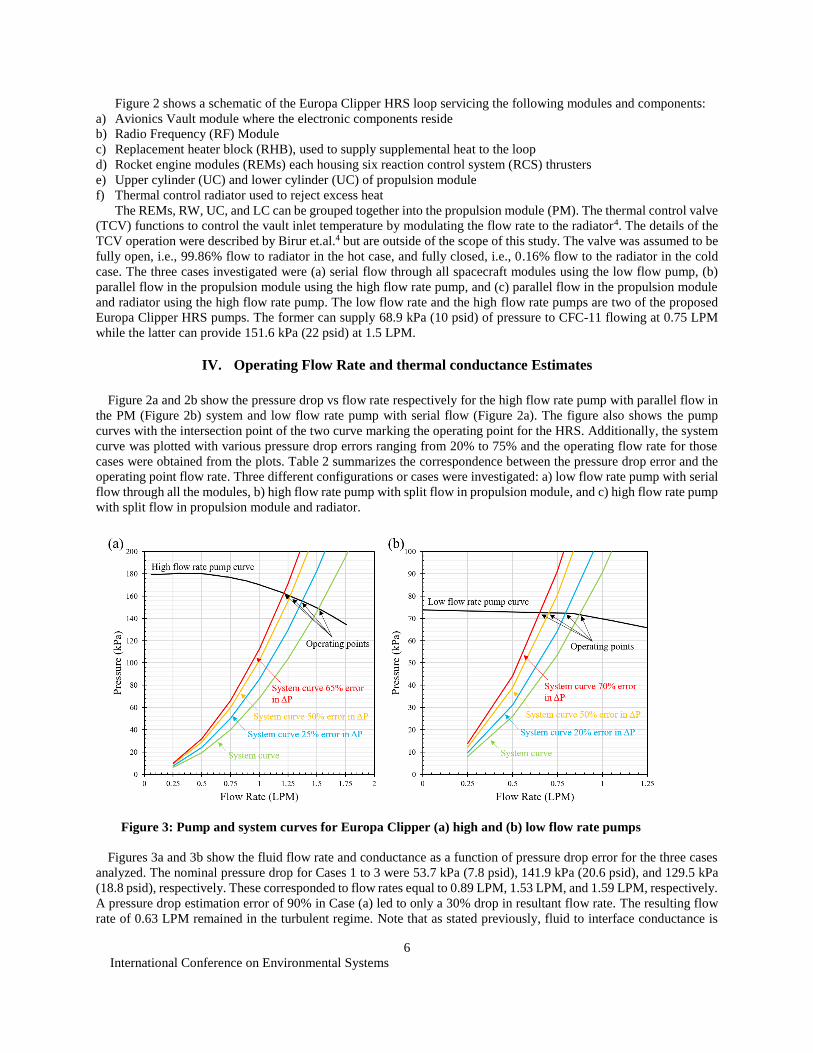
Figure 2a and 2b show the pressure drop vs flow rate respectively for the high flow rate pump with parallel flow in

the PM (Figure 2b) system and low flow rate pump with serial flow (Figure 2a). The figure also shows the pump

curves with the intersection point of the two curve marking the operating point for the HRS. Additionally, the system

curve was plotted with various pressure drop errors ranging from 20% to 75% and the operating flow rate for those

cases were obtained from the plots. Table 2 summarizes the correspondence between the pressure drop error and the

operating point flow rate. Three different configurations or cases were investigated: a) low flow rate pump with serial

flow through all the modules, b) high flow rate pump with split flow in propulsion module, and c) high flow rate pump

with split flow in propulsion module and radiator.

Figures 3a and 3b show the fluid flow rate and conductance as a function of pressure drop error for the three cases

analyzed. The nominal pressure drop for Cases 1 to 3 were 53.7 kPa (7.8 psid), 141.9 kPa (20.6 psid), and 129.5 kPa

(18.8 psid), respectively. These corresponded to flow rates equal to 0.89 LPM, 1.53 LPM, and 1.59 LPM, respectively.

A pressure drop estimation error of 90% in Case (a) led to only a 30% drop in resultant flow rate. The resulting flow

rate of 0.63 LPM remained in the turbulent regime. Note that as stated previously, fluid to interface conductance is

Figure 3: Pump and system curves for Europa Clipper (a) high and (b) low flow rate pumps


7

significantly larger for turbulent flow than laminar. Moreover, the fluid to interface conductance decreased from 11.6

to 8.8 W/m.K. For Case (b), a 60% error in the pressure drop caused the flow rate to decrease from 1.53 LPM to 1.25

LPM. Note that, the flow rate was 0.63 LPM in the propulsion module where the flow was split. The corresponding

conductance 𝐺 decreased from 18.6 W/m.K to 15.5 W/m.K due to the decrease in the flow rate. Similarly, this resulted

in a reduction in the conductance of 13% in the PM compared to its nominal value of 10.1 W/m.K at 1.5 LPM. Finally,

for Case (c) a 70% pressure drop error led to a 20% reduction in flow rate reducing conductance value from 19.2 to

15.7 W/m.K. All these cases illustrate the relatively small impact of the pressure drop error on the resultant flow rate

and the fluid to interface thermal conductance. This suggests the Europa Clipper HRS design is robust with respect to

future changes in design and errors in the pressure drop estimates.

Table 2: Example impacts of Pressure drop error on flow rates & Tube thermal conductances

Operating Cases % ΔP Error Flow Rate V Conductance G

a Low flow rate pump 0% 0.89 LPM 11.6 W/m-C

90% 0.63 LPM 8.8 W/m-C

b High Flow rate pump with split PM 0% 1.53 LPM 18.6 W/m-C

60% 1.25 LPM 15.5 W/m-C

c High flow rate pump with split PM

and radiator

0% 1.59 LPM 19.2 W/m-C

70% 1.27 LPM 15.7 W/m-C

Figure 4: (a) Fluid to interface conductance and (b) flow rate as a function of pressure drop error for low flow

rate pump, high flow rate pump with split flow in the PM, and high flow rate pump with split flow in PM and

radiator.

V. Spreadsheet for computing ΔP, Flow Rate & Thermal Conductances

To facilitate rapid calculations of the various parameters like ΔP, flow rate, and thermal conductances, a Microsoft

Excel® spreadsheet was created with built in macros to automatically estimate pressure drop, flow rate, and thermal


8

conductance for high and low flow rate pump, different ΔP errors, as well as different fluid routing. A macro button

starts the calculations after inserting above parameters in the appropriate cells. All relevant ΔPs, flow rates and thermal

conductances are tabulated and plotted (as delineated before) as outputs. Flags are provided to warn the user of laminar

flow, which would lead to low thermal conductances for large pressure drop errors.

VI. Estimating Interface Temperature Sensitivity to Pressure Drop

Once the flow rates were determined, the fluid heat capacity, �̇�𝐶𝑝 and module total thermal conductances G were

used to perform a detailed thermal model of the overall system. For each component module the fluid inlet and outlet

temperatures as well as the average interface temperature was estimated based on the heat transfer rate Q and the

total conductance G. Two thermally bounding cases were analyzed for Case b (Figure 2b), a worst case hot at 0.65

AU and a worst case cold at 5.6 AU. Figure 5 and Figure 6 respectively present the block diagrams of HRS for WCH

and WCC conditions along with the heat inputs and outputs for each module as well as fluid and interface temperatures

for Case (b) with nominal pressure drop. The fluid temperature range was between 0.2 oC and 25.9 oC and the PM

interfaces were maintained within their allowable flight temperatures of 0 oC and 35 oC in both WCH and WCC.

Moreover, the radiator was maintained 15 oC above the CFC-11 freezing point at -95 oC in WCC to limit heat loss

through the radiator to less than 10 W. Finally, the Vault was maintained within its allowable flight temperature range

of -15 oC to 45 oC.

Figure 5: Schematic of heat balance and temperature for Case (b) for worst-case hot conditions


9

Figure 6: Schematic of heat balance and temperature for Case (b) for worst-case cold conditions

VII. Assessing Worst Case Conditions at different pressure drop errors

Figure 7a and 7b show increase in WCH interface temperatures and WCC heater power as a function of increasing

pressure drop error. They illustrate that Europa Clipper HRS design is robust with respect to pressure drop. Indeed, a

75% error in ΔP for Case (b), i.e., high flow rate pump with spit PM, resulted in less than 2 oC increase in interface

temperatures compared to the nominal interface temperatures. Moreover, a 90% error in ΔP for Case (a), low flow

rate pump with serial flow through the system, resulted in less than 5 oC increase in interface temperatures compared

to the nominal values. In addition, a linear increase in ΔT vs. pressure drop was observed when the flow was in

turbulent regime. However, a sharp increase in interface temperatures was observed when flow became laminar in

both Case (a) and Case (c) due to the smaller fluid to interface heat transfer conductance associated with laminar flow

compared to turbulent regime.

Survival heater power needed to maintain the HRS controlled interfaces at their minimum AFTs increased linearly

with increasing pressure drop error. This was due to two different effects: 1) smaller fluid to interface conductance,

i.e., higher average fluid loop temperature was necessary to maintain minimum AFTs resulting in additional heat loss

and 2) the HRS operated at higher temperature and with a larger temperature gradient across the loop due to the smaller

heat capacity of the fluid �̇�𝐶𝑝 in the system with larger pressure drop.

On the other hand, low flow rate system (Case a) required more heater power compared to high flow rate system

(Case b and c) for the same ΔP error. The increase in survival heater power as a function of ΔP error is smaller for

high flow rate Cases than for low flow rate Case regardless of radiator routing. Indeed, in WCC the radiator is bypassed

completely and has no impact on loop performance. Indeed, heater power 𝑄ℎ𝑒𝑎𝑡𝑒𝑟 increased by less than 3 W (<2.5%)

due to 75% increase in pressure drop.


10

VII. Conclusions

A comprehensive case study of the effect of pressure drop increases on the overall thermal performance of a

mechanically pumped fluid loop was conducted on the Clipper HRS, and the key finding was that it was very robust

to accommodating significant pressure drop increases above the nominal estimated values. Pressure drop increases

of as much as 60% to 90% above the most conservative values lead to relatively small reductions in margins against

max allowable temperature limits. For cold conditions, this would also translate to relatively small increases in

required survival heater powers to maintain component temperatures above their minimum allowable limits. Hence,

this study gives confidence in the robustness of the fluid loop’s thermal performance to pressure drop increases either

due to the fidelity of the estimating process or due to the inevitable changes in the spacecraft configuration as the

design matures. It also dispels the notion that pressure drop is a “wall” which is impermeable or cannot be crossed

without very adverse impacts. The consequent flow regime being laminar - because of excessive pressure drops

leading to smaller flow rates - is more drastic in consequence (more of a “wall”) due to the much lower heat transfer

coefficients (thermal coupling between fluid and tubing walls) that could lead to large increases in controlled interface

temperatures. Even though this was a case study for a specific configuration (Europa Clipper), the methodology

presented in this paper and the general conclusions can be utilized for different configurations that utilize single phase

mechanically pumped fluid loops for their thermal control.

VIII. Acknowledgments

The development described in this paper was carried out at the Jet Propulsion Laboratory, California Institute of

Technology, under a contract with the National Aeronautics and Space Administration. The authors express their

thanks to Brian Carroll at JPL for data provided on measured pressure drop impedances for miscellaneous

components (mechanical fittings, flex lines, etc.) from past and current missions. Reference herein to any specific

commercial product, process, or service by trade name, trademark, manufacturer, or otherwise, does not constitute or

imply its endorsement by the United States Government or the Jet Propulsion Laboratory, California Institute of

Technology. Copyright 2018 California Institute of Technology. Government sponsorship acknowledged.

Figure 7: Effect of pressure drop error on (a) maximum interface temperature increase in WCH

conditions and (b) increase in survival heat for WCC conditions for Europa Clipper HRS controlled

component


11

IX. References 1

T. T. Lam, G. Birur and P. Bhandari, "Pumped Fluid Loops," in Spacecraft Thermal Control Handbook, El

Segundo, CA, The Aerospace Press, 2002, pp. 405-472. 2 A. Mills and C. Coimbra, Heat Transfer, San Diego, CA: Temporal Publishing, 2016. 3 R. Pappalardo, D. Senske, H. Korth, R. Klima, S. Vance and K. Craft, "The Europa Clipper Mission: Exploring

The Habilatbility of A Unique Icy World," in European Planetary Science Congress, Berlin, Germany, 2017. 4 G. Birur, M. Prina, P. Bhandari, P. Karlman, B. Hernandez, B. Kinter, P. Wilson, D. Bame and Ganapathi,

"Applications, Development of Passively Actuated Thermal Control Valves for Passive Control of Mechanically

Pumped Single-Phase Fluid Loops for Space," in International Conference on Environmental Systems, San

Francisco, CA, 2008.

Documents

Impact of Fluid Flow Pressure drop on Temperature of